The Hidden Convexity of Spectral Clustering

Abstract

In recent years, spectral clustering has become a standard method for data analysis used in a broad range of applications. In this paper we propose a new class of algorithms for multiway spectral clustering based on optimization of a certain “contrast function” over the unit sphere. These algorithms, partly inspired by certain Independent Component Analysis techniques, are simple, easy to implement and efficient.

Geometrically, the proposed algorithms can be interpreted as hidden basis recovery by means of function optimization. We give a complete characterization of the contrast functions admissible for provable basis recovery. We show how these conditions can be interpreted as a “hidden convexity” of our optimization problem on the sphere; interestingly, we use efficient convex maximization rather than the more common convex minimization. We also show encouraging experimental results on real and simulated data.

keywords: spectral clustering, convex maximization, basis recovery

1 Introduction

Partitioning a dataset into classes based on a similarity between data points, known as cluster analysis, is one of the most basic and practically important problems in data analysis and machine learning. It has a vast array of applications from speech recognition to image analysis to bioinformatics and to data compression. There is an extensive literature on the subject, including a number of different methodologies as well as their various practical and theoretical aspects [11].

In recent years spectral clustering—a class of methods based on the eigenvectors of a certain matrix, typically the graph Laplacian constructed from data—has become a widely used method for cluster analysis. This is due to the simplicity of the algorithm, a number of desirable properties it exhibits and its amenability to theoretical analysis. In its simplest form, spectral bi-partitioning is an attractively straightforward algorithm based on thresholding the second bottom eigenvector of the Laplacian matrix of a graph. However, the more practically significant problem of multiway spectral clustering is considerably more complex. While hierarchical methods based on a sequence of binary splits have been used, the most common approaches use $k$-means or weighted $k$-means clustering in the spectral space or related iterative procedures [17, 15, 2, 25]. Typical algorithms for multiway spectral clustering follow a two-step process:

1. Spectral embedding: A similarity graph for the data is constructed based on the data’s feature representation. If one is looking for $k$ clusters, one constructs the embedding using the bottom $k$ eigenvectors of the graph Laplacian (normalized or unnormalized) corresponding to that graph.

2. Clustering: In the second step, the embedded data (sometimes rescaled) is clustered, typically using the conventional/spherical $k$-means algorithms or their variations.

In the first step, the spectral embedding given by the eigenvectors of Laplacian matrices has a number of interpretations. The meaning can be explained by spectral graph theory as relaxations of multiway cut problems [19]. In the extreme case of a similarity graph having $k$ connected components, the embedded vectors reside in $\mathbb{R}^{k}$, and vectors corresponding to the same connected component are mapped to a single point. There are also connections to other areas of machine learning and mathematics, in particular to the geometry of the underlying space from which the data is sampled [4].

We propose a new class of algorithms for the second step of multiway spectral clustering. The starting point is that when the $k$ clusters are perfectly separate, the spectral embedding using the bottom $k$ eigenvectors has a particularly simple geometric form. For the unnormalized (or asymmetric normalized) Laplacian, it is simply a (weighted) orthogonal basis in $k$-dimensional space, and recovering the basis vectors is sufficient for cluster identification. This view of spectral clustering as basis recovery is related to previous observations that the spectral embedding generates a discrete weighted simplex (see [21, 12] for some applications). For the symmetric normalized Laplacian, the structure is slightly more complex, but is still suitable for our analysis. Moreover, our proposed algorithms can be used without modification.

The proposed approach relies on an optimization problem resembling certain Independent Component Analysis techniques, such as FastICA (see [10] for a broad overview). Specifically, the problem of identifying $k$ clusters reduces to maximizing a certain “admissible” contrast function over a $(k-1)$-sphere. Our main theoretical contribution is to formulate a general version of the basis recovery problem arising in spectral clustering, and to characterize the set of admissible contrast functions for guaranteed recovery (Section 2). Rather than the more usual convex minimization, our analysis is based on convex maximization over a (hidden) convex domain. Interestingly, while maximizing a convex function over a convex domain is generally difficult (even maximizing a positive definite quadratic form over the continuous cube $[0,1]^{n}$ is NP-hard), our setting allows for efficient optimization.

Based on this theoretical connection between clusters and local maxima of contrast functions over the sphere, we propose practical algorithms for cluster recovery through function maximization. We discuss the choice of contrast functions and provide running time analysis. We also provide a number of encouraging experimental results on synthetic and real-world data sets.

We also note connections to recent work on geometric recovery. Anderson et al. [1] use the method of moments to recover a continuous simplex given samples from the uniform probability distribution. Like in our work, Anderson et al. use efficient enumeration of local maxima of a function over the sphere. Also, one of the results of Hsu and Kakade [9] shows recovery of parameters in a Gaussian Mixture Model using the moments of order three, and this result can be thought of as a case of the basis recovery problem.

The paper is structured as follows: In Section 2, we provide our main technical results on basis recovery and briefly outline its connection to spectral clustering. In Sections 3 and 4 we introduce spectral clustering and formulate it in terms of basis learning. In Section 5 we provide the main theoretical results for basis recovery in the spectral clustering setting, and discuss algorithic implementation details. Our experimental results are given in Section 6. Finally in Section 7, we handle the deferred proof details and discuss the admissibility of normalized graph Laplacians for our framework.

2 Basis Recovery and Spectral Clustering

In this section, we provide our main technical results on hidden basis recovery. Then, we briefly discuss how our results will apply to the spectral clustering setting.

A Note on Notation. In what follows, we will use the following notations. For a matrix $B$, $b_{ij}$ indicates the element in its $i$^th row and $j$^th column. The $i$^th row vector of $B$ is denoted $b_{i\mathchoice{{\hbox to5.05554pt{\hss\leavevmode\hbox{\raisebox{0.0pt}{\scalebox{0.5}{\raisebox{0.0pt}{$\displaystyle\bullet$}}}}\hss}}}{{\hbox to5.05554pt{\hss\leavevmode\hbox{\raisebox{0.0pt}{\scalebox{0.5}{\raisebox{0.0pt}{$\textstyle\bullet$}}}}\hss}}}{{\hbox to4.00554pt{\hss\leavevmode\hbox{\raisebox{0.0pt}{\scalebox{0.5}{\raisebox{0.0pt}{$\scriptstyle\bullet$}}}}\hss}}}{{\hbox to3.30554pt{\hss\leavevmode\hbox{\raisebox{0.0pt}{\scalebox{0.5}{\raisebox{0.0pt}{$\scriptscriptstyle\bullet$}}}}\hss}}}}$, and the $j$^th column vector of $B$ is denoted $b_{\mathchoice{{\hbox to5.05554pt{\hss\leavevmode\hbox{\raisebox{0.0pt}{\scalebox{0.5}{\raisebox{0.0pt}{$\displaystyle\bullet$}}}}\hss}}}{{\hbox to5.05554pt{\hss\leavevmode\hbox{\raisebox{0.0pt}{\scalebox{0.5}{\raisebox{0.0pt}{$\textstyle\bullet$}}}}\hss}}}{{\hbox to4.00554pt{\hss\leavevmode\hbox{\raisebox{0.0pt}{\scalebox{0.5}{\raisebox{0.0pt}{$\scriptstyle\bullet$}}}}\hss}}}{{\hbox to3.30554pt{\hss\leavevmode\hbox{\raisebox{0.0pt}{\scalebox{0.5}{\raisebox{0.0pt}{$\scriptscriptstyle\bullet$}}}}\hss}}}j}$. For a vector $\mathbf{v}$, $\lVert\mathbf{v}\rVert$ denotes its standard Euclidean 2-norm. Given two vectors $\mathbf{u}$ and $\mathbf{v}$, $\mathbf{u}\mathbin{\mathchoice{{\hbox to7.22218pt{\hss\leavevmode\hbox{\raisebox{0.0pt}{\scalebox{0.5}{\raisebox{0.0pt}{$\displaystyle\bullet$}}}}\hss}}}{{\hbox to7.22218pt{\hss\leavevmode\hbox{\raisebox{0.0pt}{\scalebox{0.5}{\raisebox{0.0pt}{$\textstyle\bullet$}}}}\hss}}}{{\hbox to5.72217pt{\hss\leavevmode\hbox{\raisebox{0.0pt}{\scalebox{0.5}{\raisebox{0.0pt}{$\scriptstyle\bullet$}}}}\hss}}}{{\hbox to4.72217pt{\hss\leavevmode\hbox{\raisebox{0.0pt}{\scalebox{0.5}{\raisebox{0.0pt}{$\scriptscriptstyle\bullet$}}}}\hss}}}}\mathbf{v}$ denotes their dot product. We denote the set $\{1,2,\dotsc,k\}$ by $[k]$. We denote by $\mathbf{1}_{\mathcal{S}}$ the indicator vector for the set $\mathcal{S}$, i.e. the vector which is $1$ for indices in $\mathcal{S}$ and $0$ otherwise. The null space of a matrix $M$ is denoted $\mathcal{N}(M)$. We denote the unit sphere in $\mathbb{R}^{d}$ by $\mathbb{S}^{d-1}$. For points $p_{1},\dotsc,p_{m}$, $\operatorname{conv}(p_{1},\dotsc,p_{m})$ will denote their convex hull. All angles are given in radians, and $\angle(\mathbf{u},\mathbf{v})$ denotes the angle between the vectors $\mathbf{u}$ and $\mathbf{v}$ in the domain $[0,\pi]$. We use $\mapsto$ to define anonymous functions; for instance $t\mapsto t^{2}$ is the function $f:\mathbb{R}\rightarrow\mathbb{R}$ defined by $f(t):=t^{2}$. Finally, for $\mathcal{X}$ a subspace of $\mathbb{R}^{d}$, $P_{\mathcal{X}}$ denotes the square matrix corresponding to the orthogonal projection from $\mathbb{R}^{d}$ to $\mathcal{X}$.

2.1 Basis Recovery via Convex Maximization

The main technical results of this section deal with reconstructing a hidden basis by simple optimization techniques. For this purpose, we introduce the following class of functions.

Definition 1.

A function $F:\mathbb{R}^{d}\rightarrow\mathbb{R}$ is said to be an orthogonal basis encoding function (orthogonal BEF) if there exists an orthonormal basis $\mathbf{z}_{1},\dotsc,\mathbf{z}_{d}$ of $\mathbb{R}^{d}$ and functions $g_{i}:\mathbb{R}\rightarrow\mathbb{R}$ such that $F(\mathbf{u})=\sum_{i=1}^{d}g_{i}(\mathbf{u}\mathbin{\mathchoice{{\hbox to7.22218pt{\hss\leavevmode\hbox{\raisebox{0.0pt}{\scalebox{0.5}{\raisebox{0.0pt}{$\displaystyle\bullet$}}}}\hss}}}{{\hbox to7.22218pt{\hss\leavevmode\hbox{\raisebox{0.0pt}{\scalebox{0.5}{\raisebox{0.0pt}{$\textstyle\bullet$}}}}\hss}}}{{\hbox to5.72217pt{\hss\leavevmode\hbox{\raisebox{0.0pt}{\scalebox{0.5}{\raisebox{0.0pt}{$\scriptstyle\bullet$}}}}\hss}}}{{\hbox to4.72217pt{\hss\leavevmode\hbox{\raisebox{0.0pt}{\scalebox{0.5}{\raisebox{0.0pt}{$\scriptscriptstyle\bullet$}}}}\hss}}}}\mathbf{z}_{i})$.

We will assume throughout that the functions $g_{i}$ (and hence $F$) are continuously differentiable. In this section, we provide conditions under which recovery of the hidden basis $\mathbf{z}_{1},\dotsc,\mathbf{z}_{d}$ (up to sign) can be guaranteed for an orthogonal BEF using simple function maximization techniques. To motivate our conditions, it will be useful to first consider a classic problem which fits into the orthogonal BEF framework: the eigendecomposition of positive definite symmetric matrices.

Example 2 (Symmetric PSD Matrix Eigendecompositions).

Let $A$ be a symmetric positive semi-definite matrix with eigendecomposition $A=\sum_{i=1}^{d}\lambda_{i}\mathbf{z}_{i}\mathbf{z}_{i}^{T}$. The function $F_{A}:\mathbb{R}^{d}\rightarrow\mathbb{R}$ defined by $F_{A}(\mathbf{u}):=\mathbf{u}^{T}A\mathbf{u}=\sum_{i=1}^{d}\lambda_{i}(\mathbf{u}\mathbin{\mathchoice{{\hbox to7.22218pt{\hss\leavevmode\hbox{\raisebox{0.0pt}{\scalebox{0.5}{\raisebox{0.0pt}{$\displaystyle\bullet$}}}}\hss}}}{{\hbox to7.22218pt{\hss\leavevmode\hbox{\raisebox{0.0pt}{\scalebox{0.5}{\raisebox{0.0pt}{$\textstyle\bullet$}}}}\hss}}}{{\hbox to5.72217pt{\hss\leavevmode\hbox{\raisebox{0.0pt}{\scalebox{0.5}{\raisebox{0.0pt}{$\scriptstyle\bullet$}}}}\hss}}}{{\hbox to4.72217pt{\hss\leavevmode\hbox{\raisebox{0.0pt}{\scalebox{0.5}{\raisebox{0.0pt}{$\scriptscriptstyle\bullet$}}}}\hss}}}}\mathbf{z}_{i})^{2}$ is an orthogonal BEF with the functions $g_{i}:\mathbb{R}\rightarrow\mathbb{R}$ defined as $g_{i}(x):=\lambda_{i}x^{2}$. If the eigenvalues are ordered such that $\lambda_{1}>\lambda_{2}>\dotsc>\lambda_{d}$, then the directions $\pm\mathbf{z}_{1}$ are the maxima (local and global) of $F_{A}$ on the domain $\mathbb{S}^{d-1}$. Further, after $\pm\mathbf{z}_{1}$ is recovered, we may maximize $F_{A}$ in the orthogonal complement of $\mathbf{z}_{1}$ to recover $\pm\mathbf{z}_{2}$. This deflationary procedure can be extended to recover all eigenvectors of $F_{A}$ (see Algorithm 1 for the idea).

However, when $A$ has repeated eigenvalues, then its eigendecomposition is no longer uniquely defined. For the identity matrix $\mathcal{I}$, any orthonormal basis in $\mathbb{R}^{d}$ can be used to form its eigenvectors, and the function $F_{\mathcal{I}}(\mathbf{u})=1$ for any choice of $\mathbf{u}\in\mathbb{S}^{d-1}$. In general, the hidden basis recovery problem arising in the eigendecomposition problem is only uniquely defined when there are no repeat eigenvalues.

As pointed out by the Example 2, we will need to understand the conditions under which a deflationary approach to maximizing a BEF $F$ on $\mathbb{S}^{d-1}$ (see Algorithm 1) can be guaranteed to recover the hidden basis $\mathbf{z}_{1},\dotsc,\mathbf{z}_{d}$. We also wish that the hidden basis $\mathbf{z}_{1},\dotsc,\mathbf{z}_{d}$ be uniquely defined by the BEF $F$. It turns out that the following assumption is sufficient for performing guaranteed basis recovery.

Assumption 3 (Strict convexity).

For all $i\in[d]$, $t\mapsto g_{i}(\operatorname{sign}(t)\sqrt{{|t|}})$ is strictly convex.

More formally, we have the following result.

Algorithm 1 The deflationary scheme for hidden basis recovery. This is an abstract algorithm which when given access to an orthogonal BEF $F(\mathbf{u})=\sum_{i=1}^{d}g_{i}(\mathbf{u}\mathbin{\mathchoice{{\hbox to7.22218pt{\hss\leavevmode\hbox{\raisebox{0.0pt}{\scalebox{0.5}{\raisebox{0.0pt}{$\displaystyle\bullet$}}}}\hss}}}{{\hbox to7.22218pt{\hss\leavevmode\hbox{\raisebox{0.0pt}{\scalebox{0.5}{\raisebox{0.0pt}{$\textstyle\bullet$}}}}\hss}}}{{\hbox to5.72217pt{\hss\leavevmode\hbox{\raisebox{0.0pt}{\scalebox{0.5}{\raisebox{0.0pt}{$\scriptstyle\bullet$}}}}\hss}}}{{\hbox to4.72217pt{\hss\leavevmode\hbox{\raisebox{0.0pt}{\scalebox{0.5}{\raisebox{0.0pt}{$\scriptscriptstyle\bullet$}}}}\hss}}}}\mathbf{z}_{i})$ satisfying Assumption 3, it recovers and returns estimates of the hidden basis directions $\mathbf{z}_{1},\dotsc,\mathbf{z}_{d}$ up to unknown signs and potentially an unknown permutation.

1:for $i\leftarrow 1$ to $d$ do

2:     Find $\tilde{}\mathbf{z}_{i}$ a local maximizer of $F$ on $\mathbb{S}^{d-1}\cap\operatorname{span}(\{\tilde{}\mathbf{z}_{1},\tilde{}\mathbf{z}_{2},\dotsc,\tilde{}\mathbf{z}_{i-1}\})^{\perp}$

3:end for

4:return $\tilde{}\mathbf{z}_{1},\dotsc,\tilde{}\mathbf{z}_{d}$.

Theorem 4.

Suppose that $F$ is an orthogonal BEF satisfying Assumption 3. Then, the set of local maxima of $F$ on the unit sphere is non-empty and contained in the set $\{\pm\mathbf{z}_{1},\dotsc,\pm\mathbf{z}_{d}\}$.

The Assumption 3 is sufficient for hidden basis recovery in the sense of the following Corollary. Its proof is an exercise in induction on the number of recovered vectors $\tilde{}\mathbf{z}_{j}$, where the inductive step is a result of Theorem 4.

Corollary 5.

If $F$ is an orthogonal BEF satisfying Assumption 3, then the abstract Algorithm 1 returns vectors $\tilde{}\mathbf{z}_{1},\dotsc,\tilde{}\mathbf{z}_{d}$ which recover the directions $\mathbf{z}_{1},\dotsc,\mathbf{z}_{d}$ up to a choice of signs and permutation. More precisely, there exists sign $s_{i}\in\{\pm 1\}$ and a permutation $p$ of $[d]$ such that $\mathbf{z}_{i}=s_{i}\tilde{}\mathbf{z}_{p(i)}$ for each $i\in[d]$.

Before proceding with the proof of Theorem 4, it is worth discussing the importance of strict convexity in Assumption 3. In the case of the matrix eigendecomposition Example 2 with the identity matrix $\mathcal{I}$, we constructed an orthogonal BEF with contrast functions $g_{i}(t)=t^{2}$ which satisfy that each $g_{i}(\operatorname{sign}(t)\sqrt{{|t|}})=t$ is convex but not strictly convex. The function $F_{\mathcal{I}}(\mathbf{u})$ is constant on the unit sphere, and there is no uniquely defined hidden basis (or eigenvector basis) for the identity matrix. In this sense, it does not suffice for $t\mapsto g(\operatorname{sign}(t)\sqrt{{|t|}})$ to be convex.

Interestingly, the only issue which can arise when strict convexity is relaxed to convexity in Assumption 3 is that the function $F$ may plateau (become constant) on regions within the unit sphere $\mathbb{S}^{d-1}$. Strict convexity is one way to ensure that this does not happen. Nevertheless, the problem of recovering the eigendecomposition of a positive definite symmetric matrix $A$ (Example 2) is a limit case of our framework. Moreover, Algorithm 1 can be used to perform eigenvector recovery since one does not require uniqueness of the eigenvector basis.

The intuition behind Assumption 3 is captured in the proof of Theorem 4. The main idea is to introduce a change of variable and recast maximization of $F$ over the unit sphere as a convex maximization problem defined over a (hidden) convex domain.

Proof of Theorem 4.

We will use the following Fact about convex maximization (see [16, Chapter 32] for an overview of concepts related to convex maximization).

For a convex set $K$, a point $x\in K$ is said to be an extreme point if $x$ is not equal to a strict convex combination of two other points in $K$.

Fact 6.

Suppose that $K$ is a closed and bounded convex set. Let $f:K\rightarrow\mathbb{R}$ be a strictly convex function. Then, the set of local maxima of $f$ on $K$ is non-empty and contained in the set of extreme points of $K$.

As $\mathbf{z}_{1},\dotsc,\mathbf{z}_{d}$ form an orthonormal basis of the space, we may simplify notation and work in the coordinate system in which $\mathbf{z}_{1},\dotsc,\mathbf{z}_{d}$ are the canonical vectors $\mathbf{e}_{1},\dotsc,\mathbf{e}_{d}$. We define $\Delta^{d-1}:=\operatorname{conv}(\mathbf{e}_{1},\dotsc,\mathbf{e}_{d})$ a (hidden) simplex, and $Q_{+}^{d-1}:=\{\mathbf{u}\in\mathbb{S}^{d}\mathrel{|}u_{i}\geq 0\text{ for all }i\in[d]\}$ the restriction of the sphere onto the positive orthant. By the symmetries of the problem, it suffices to show that the set $S$ of local maxima of $F$ with respect to $Q_{+}^{d-1}$ is non-empty and that $S\subset\{\mathbf{e}_{1},\dotsc,\mathbf{e}_{d}\}$.

The main idea is to use the change of variable $\psi:Q_{+}^{d-1}\rightarrow\Delta^{d-1}$ defined by $\psi_{i}(\mathbf{u})=u_{i}^{2}$. Since

$$F\circ\psi^{-1}(\mathbf{x})=\sum_{i=1}^{d}g_{i}(\psi^{-1}_{i}(\mathbf{x}))=\sum_{i=1}^{d}g_{i}(\sqrt{x_{i}})\ ,$$ (1)

then by Assumption 3, $F\circ\psi^{-1}:\Delta^{d-1}\rightarrow\mathbb{R}$ is a strictly convex function defined on a closed and bounded convex domain. By Fact 6, we note that the set $S^{\prime}$ of local maxima of $F\circ\psi^{-1}$ on $\Delta^{d-1}$ is nonempty and contained in the set $\{\mathbf{e}_{1},\dotsc,\mathbf{e}_{d}\}$ of extreme points of $\Delta^{d-1}$. Pulling back to $Q_{+}^{d-1}$, we see that $S=\psi^{-1}(S^{\prime})$ is a non-empty subset of $\{\mathbf{e}_{1},\dotsc,\mathbf{e}_{d}\}$. ∎

2.2 Spectral Clustering as Basis Recovery

It turns out that orthogonal basis recovery has direct implications for spectral clustering. In particular, when an $n$-vertex similarity graph $G$ has $k$ connected components corresponding to the desired clusters, it will be seen in section 4 that the spectral embedding into $\mathbb{R}^{k}$ maps each vertex $\mathbf{v}_{i}$ in the $j$^th connected component onto a ray protruding from the origin in a direction $\mathbf{z}_{j}$. It happens that the directions $\mathbf{z}_{1},\dotsc,\mathbf{z}_{k}$ are orthogonal. We let $\mathbf{x}_{i}$ denote the embedded points and we construct the function

$$F_{g}(\mathbf{u}):=\frac{1}{n}\sum_{i=1}^{n}g({|\mathbf{u}\mathbin{\mathchoice{{\hbox to7.22218pt{\hss\leavevmode\hbox{\raisebox{0.0pt}{\scalebox{0.5}{\raisebox{0.0pt}{$\displaystyle\bullet$}}}}\hss}}}{{\hbox to7.22218pt{\hss\leavevmode\hbox{\raisebox{0.0pt}{\scalebox{0.5}{\raisebox{0.0pt}{$\textstyle\bullet$}}}}\hss}}}{{\hbox to5.72217pt{\hss\leavevmode\hbox{\raisebox{0.0pt}{\scalebox{0.5}{\raisebox{0.0pt}{$\scriptstyle\bullet$}}}}\hss}}}{{\hbox to4.72217pt{\hss\leavevmode\hbox{\raisebox{0.0pt}{\scalebox{0.5}{\raisebox{0.0pt}{$\scriptscriptstyle\bullet$}}}}\hss}}}}\mathbf{x}_{i}|})\ ,$$

from the embedded data and the contrast function $g:\mathbb{R}\rightarrow\mathbb{R}$.

To see that $F_{g}$ is actually an orthogonal BEF, we consider the following theoretical construction: Let $\SS_{1},\dotsc\SS_{k}$ be the vertex index sets corresponding to the distinct components of the graph $G$, and define the functions $g_{j}:\mathbb{R}\rightarrow\mathbb{R}$ for all $j\in[k]$ by $g_{j}(t)=\frac{1}{n}\sum_{i\in\SS_{j}}g(t\lVert\mathbf{x}_{i}\rVert)$. Then, it may be verified that $F_{g}(\mathbf{u})=\sum_{j=1}^{k}g_{j}(\mathbf{u}\mathbin{\mathchoice{{\hbox to7.22218pt{\hss\leavevmode\hbox{\raisebox{0.0pt}{\scalebox{0.5}{\raisebox{0.0pt}{$\displaystyle\bullet$}}}}\hss}}}{{\hbox to7.22218pt{\hss\leavevmode\hbox{\raisebox{0.0pt}{\scalebox{0.5}{\raisebox{0.0pt}{$\textstyle\bullet$}}}}\hss}}}{{\hbox to5.72217pt{\hss\leavevmode\hbox{\raisebox{0.0pt}{\scalebox{0.5}{\raisebox{0.0pt}{$\scriptstyle\bullet$}}}}\hss}}}{{\hbox to4.72217pt{\hss\leavevmode\hbox{\raisebox{0.0pt}{\scalebox{0.5}{\raisebox{0.0pt}{$\scriptscriptstyle\bullet$}}}}\hss}}}}\mathbf{z}_{j})$, which takes on the form of an orthogonal BEF. In particular, we will be able to recover the directions $\mathbf{z}_{1},\dotsc,\mathbf{z}_{k}$ corresponding to the desired clusters by maximizing the function $F_{g}$ on the unit sphere $\mathbb{S}^{k-1}$.

Due to the special form of orthogonal BEF which arises in spectral clustering, we will have slightly stronger guarantees. In particular, it will be seen (Theorem 9 and Theorem 18) all of the directions of $\pm\mathbf{z}_{1},\dotsc,\pm\mathbf{z}_{k}$ are strict local maximum of $F_{g}$ on $\mathbb{S}^{k-1}$ instead of just some.

3 Spectral Clustering Problem Statement

Let $G=(V,A)$ denote a similarity graph where $V$ is a set of $n$ vertices and $A$ is an adjacency matrix with non-negative weights. Two vertices $i,j\in V$ are incident if $a_{ij}>0$, and the value of $a_{ij}$ is interpreted as a measure of the similarity between the vertices. In spectral clustering, the goal is to partition the vertices of a graph into sets $\mathcal{S}_{1},\dotsc,\mathcal{S}_{k}$ such that these vertex sets form natural clusters in the graph. In the most basic setting, $G$ consists of $k$ connected components, and the natural clusters should be the components themselves. In this case, if $i^{\prime}\in\mathcal{S}_{i}$ and $j^{\prime}\in\mathcal{S}_{j}$ then $a_{i^{\prime}j^{\prime}}=0$ whenever $i\neq j$. For convenience, we can consider the vertices of $V$ to be indexed such that all indices in $\mathcal{S}_{i}$ precede all indices in $\mathcal{S}_{j}$ when $i<j$. The matrix $A$ takes on the form:

$$A=\left(\begin{array}[]{cccc}A_{\mathcal{S}_{1}}&0&\cdots&0\\ 0&A_{\mathcal{S}_{2}}&\cdots&0\\ \vdots&\vdots&\ddots&\vdots\\ 0&0&\cdots&A_{\mathcal{S}_{k}}\end{array}\right)\ ,$$

a block diagonal matrix. In this setting, spectral clustering can be viewed as a technique for reorganizing a given similarity matrix $A$ into such a block diagonal matrix.

In practice, $G$ rarely consists of $k$ truly disjoint connected components. Instead, one typically observes a matrix $\tilde{A}=A+E$ where $E$ is a perturbation from the clean setting. The goal of spectral clustering is to permute the rows and columns of $\tilde{A}$ to form a matrix which is nearly block diagonal and to recover the corresponding clusters.

4 The Spectral Embedding

Given an $n$-vertex similarity graph $G=(V,A)$, let $D$ be the diagonal degree matrix with non-zero entries $d_{ii}=\sum_{j\in V}a_{ij}$. The graph Laplacian is defined as $L:=D-A$. The following well known property of the graph Laplacian (see [19] for a review) helps shed light on its importance: Given $\mathbf{u}\in\mathbb{R}^{n}$,

$$\mathbf{u}^{T}L\mathbf{u}=\frac{1}{2}\sum_{i,j\in V}a_{ij}(u_{i}-u_{j})^{2}\ .$$ (2)

The graph Laplacian $L$ is symmetric positive semi-definite as equation (2) cannot be negative. Further, $\mathbf{u}$ is a 0-eigenvector of $L$ (or equivalently, $\mathbf{u}\in\mathcal{N}(L)$) if and only if $\mathbf{u}^{T}L\mathbf{u}=0$. When $G$ consists of $k$ connected components with indices in the sets $\mathcal{S}_{1},\dotsc,\mathcal{S}_{k}$, inspection of equation (2) gives that $\mathbf{u}\in\mathcal{N}(L)$ precisely when $\mathbf{u}$ is piecewise constant on each $\mathcal{S}_{i}$. In particular,

$$\{{|\mathcal{S}_{1}|}^{-1/2}\mathbf{1}_{\mathcal{S}_{1}},\dotsc,{|\mathcal{S}_{k}|}^{-1/2}\mathbf{1}_{\mathcal{S}_{k}}\}$$ (3)

is an orthonormal basis for $\mathcal{N}(L)$.

In general, letting $X\in\mathbb{R}^{n\times k}$ contain an orthogonal basis of $\mathcal{N}(L)$, it cannot be guaranteed that the rows of $X$ will act as indicators of the various classes, as the columns of $X$ have only been characterized up to a rotation within the subspace $\mathcal{N}(L)$. However, the rows of $X$ are contained in a scaled orthogonal basis of $\mathbb{R}^{k}$ with the basis directions corresponding to the various classes. We formulate this result as follows (see [21], [18, Proposition 5], and [15, Proposition 1] for related statements).

Proposition 7.

Let the similarity graph $G=(V,A)$ contain $k$ connected components with indices in the sets $\mathcal{S}_{1},\dotsc,\mathcal{S}_{k}$, let $n={|V|}$, and let $L$ be the graph Laplacian of $G$. Then, $\mathcal{N}(L)$ has dimensionality $k$. Let $X=(x_{\mathchoice{{\hbox to5.05554pt{\hss\leavevmode\hbox{\raisebox{0.0pt}{\scalebox{0.5}{\raisebox{0.0pt}{$\displaystyle\bullet$}}}}\hss}}}{{\hbox to5.05554pt{\hss\leavevmode\hbox{\raisebox{0.0pt}{\scalebox{0.5}{\raisebox{0.0pt}{$\textstyle\bullet$}}}}\hss}}}{{\hbox to4.00554pt{\hss\leavevmode\hbox{\raisebox{0.0pt}{\scalebox{0.5}{\raisebox{0.0pt}{$\scriptstyle\bullet$}}}}\hss}}}{{\hbox to3.30554pt{\hss\leavevmode\hbox{\raisebox{0.0pt}{\scalebox{0.5}{\raisebox{0.0pt}{$\scriptscriptstyle\bullet$}}}}\hss}}}1},\dotsc,x_{\mathchoice{{\hbox to5.05554pt{\hss\leavevmode\hbox{\raisebox{0.0pt}{\scalebox{0.5}{\raisebox{0.0pt}{$\displaystyle\bullet$}}}}\hss}}}{{\hbox to5.05554pt{\hss\leavevmode\hbox{\raisebox{0.0pt}{\scalebox{0.5}{\raisebox{0.0pt}{$\textstyle\bullet$}}}}\hss}}}{{\hbox to4.00554pt{\hss\leavevmode\hbox{\raisebox{0.0pt}{\scalebox{0.5}{\raisebox{0.0pt}{$\scriptstyle\bullet$}}}}\hss}}}{{\hbox to3.30554pt{\hss\leavevmode\hbox{\raisebox{0.0pt}{\scalebox{0.5}{\raisebox{0.0pt}{$\scriptscriptstyle\bullet$}}}}\hss}}}k})$ contain $k$ scaled, orthogonal column vectors forming a basis of $\mathcal{N}(L)$ such that $\lVert x_{\mathchoice{{\hbox to5.05554pt{\hss\leavevmode\hbox{\raisebox{0.0pt}{\scalebox{0.5}{\raisebox{0.0pt}{$\displaystyle\bullet$}}}}\hss}}}{{\hbox to5.05554pt{\hss\leavevmode\hbox{\raisebox{0.0pt}{\scalebox{0.5}{\raisebox{0.0pt}{$\textstyle\bullet$}}}}\hss}}}{{\hbox to4.00554pt{\hss\leavevmode\hbox{\raisebox{0.0pt}{\scalebox{0.5}{\raisebox{0.0pt}{$\scriptstyle\bullet$}}}}\hss}}}{{\hbox to3.30554pt{\hss\leavevmode\hbox{\raisebox{0.0pt}{\scalebox{0.5}{\raisebox{0.0pt}{$\scriptscriptstyle\bullet$}}}}\hss}}}j}\rVert=\sqrt{}n$ for each $j\in[k]$. Then, there exist weights $w_{1},\dotsc,w_{k}$ with $w_{j}=\frac{{|\mathcal{S}_{j}|}}{n}$ and mutually orthogonal vectors $\mathbf{z}_{1},\dotsc,\mathbf{z}_{k}\in\mathbb{R}^{k}$ such that whenever $i\in\mathcal{S}_{j}$, the row vector $x_{i\mathchoice{{\hbox to5.05554pt{\hss\leavevmode\hbox{\raisebox{0.0pt}{\scalebox{0.5}{\raisebox{0.0pt}{$\displaystyle\bullet$}}}}\hss}}}{{\hbox to5.05554pt{\hss\leavevmode\hbox{\raisebox{0.0pt}{\scalebox{0.5}{\raisebox{0.0pt}{$\textstyle\bullet$}}}}\hss}}}{{\hbox to4.00554pt{\hss\leavevmode\hbox{\raisebox{0.0pt}{\scalebox{0.5}{\raisebox{0.0pt}{$\scriptstyle\bullet$}}}}\hss}}}{{\hbox to3.30554pt{\hss\leavevmode\hbox{\raisebox{0.0pt}{\scalebox{0.5}{\raisebox{0.0pt}{$\scriptscriptstyle\bullet$}}}}\hss}}}}=\frac{1}{\sqrt{w_{j}}}\mathbf{z}_{j}^{T}$.

Proof.

We define the matrix $M_{\mathcal{S}_{i}}:=\mathbf{1}_{\mathcal{S}_{i}}\mathbf{1}_{\mathcal{S}_{i}}^{T}$. $P_{\mathcal{N}(L)}$ can be constructed from any orthonormal basis of $\mathcal{N}(L)$. Using the two bases $\{{|\mathcal{S}_{1}|}^{-1/2}\mathbf{1}_{\mathcal{S}_{1}},\dotsc,{|\mathcal{S}_{k}|}^{-1/2}\mathbf{1}_{\mathcal{S}_{k}}\}$ and $\{\frac{1}{\sqrt{}n}x_{\mathchoice{{\hbox to5.05554pt{\hss\leavevmode\hbox{\raisebox{0.0pt}{\scalebox{0.5}{\raisebox{0.0pt}{$\displaystyle\bullet$}}}}\hss}}}{{\hbox to5.05554pt{\hss\leavevmode\hbox{\raisebox{0.0pt}{\scalebox{0.5}{\raisebox{0.0pt}{$\textstyle\bullet$}}}}\hss}}}{{\hbox to4.00554pt{\hss\leavevmode\hbox{\raisebox{0.0pt}{\scalebox{0.5}{\raisebox{0.0pt}{$\scriptstyle\bullet$}}}}\hss}}}{{\hbox to3.30554pt{\hss\leavevmode\hbox{\raisebox{0.0pt}{\scalebox{0.5}{\raisebox{0.0pt}{$\scriptscriptstyle\bullet$}}}}\hss}}}1},\dotsc,\allowbreak\frac{1}{\sqrt{}n}x_{\mathchoice{{\hbox to5.05554pt{\hss\leavevmode\hbox{\raisebox{0.0pt}{\scalebox{0.5}{\raisebox{0.0pt}{$\displaystyle\bullet$}}}}\hss}}}{{\hbox to5.05554pt{\hss\leavevmode\hbox{\raisebox{0.0pt}{\scalebox{0.5}{\raisebox{0.0pt}{$\textstyle\bullet$}}}}\hss}}}{{\hbox to4.00554pt{\hss\leavevmode\hbox{\raisebox{0.0pt}{\scalebox{0.5}{\raisebox{0.0pt}{$\scriptstyle\bullet$}}}}\hss}}}{{\hbox to3.30554pt{\hss\leavevmode\hbox{\raisebox{0.0pt}{\scalebox{0.5}{\raisebox{0.0pt}{$\scriptscriptstyle\bullet$}}}}\hss}}}k}\}$ yields:

$$P_{\mathcal{N}(L)}=\sum_{i=1}^{k}{|\mathcal{S}_{i}|}^{-1}M_{\mathcal{S}_{i}}\quad\text{and}\quad P_{\mathcal{N}(L)}=\frac{1}{n}XX^{T}\ .$$

Thus for $i,j\in V$, $\frac{1}{n}x_{i\mathchoice{{\hbox to5.05554pt{\hss\leavevmode\hbox{\raisebox{0.0pt}{\scalebox{0.5}{\raisebox{0.0pt}{$\displaystyle\bullet$}}}}\hss}}}{{\hbox to5.05554pt{\hss\leavevmode\hbox{\raisebox{0.0pt}{\scalebox{0.5}{\raisebox{0.0pt}{$\textstyle\bullet$}}}}\hss}}}{{\hbox to4.00554pt{\hss\leavevmode\hbox{\raisebox{0.0pt}{\scalebox{0.5}{\raisebox{0.0pt}{$\scriptstyle\bullet$}}}}\hss}}}{{\hbox to3.30554pt{\hss\leavevmode\hbox{\raisebox{0.0pt}{\scalebox{0.5}{\raisebox{0.0pt}{$\scriptscriptstyle\bullet$}}}}\hss}}}}\mathbin{\mathchoice{{\hbox to7.22218pt{\hss\leavevmode\hbox{\raisebox{0.0pt}{\scalebox{0.5}{\raisebox{0.0pt}{$\displaystyle\bullet$}}}}\hss}}}{{\hbox to7.22218pt{\hss\leavevmode\hbox{\raisebox{0.0pt}{\scalebox{0.5}{\raisebox{0.0pt}{$\textstyle\bullet$}}}}\hss}}}{{\hbox to5.72217pt{\hss\leavevmode\hbox{\raisebox{0.0pt}{\scalebox{0.5}{\raisebox{0.0pt}{$\scriptstyle\bullet$}}}}\hss}}}{{\hbox to4.72217pt{\hss\leavevmode\hbox{\raisebox{0.0pt}{\scalebox{0.5}{\raisebox{0.0pt}{$\scriptscriptstyle\bullet$}}}}\hss}}}}x_{j\mathchoice{{\hbox to5.05554pt{\hss\leavevmode\hbox{\raisebox{0.0pt}{\scalebox{0.5}{\raisebox{0.0pt}{$\displaystyle\bullet$}}}}\hss}}}{{\hbox to5.05554pt{\hss\leavevmode\hbox{\raisebox{0.0pt}{\scalebox{0.5}{\raisebox{0.0pt}{$\textstyle\bullet$}}}}\hss}}}{{\hbox to4.00554pt{\hss\leavevmode\hbox{\raisebox{0.0pt}{\scalebox{0.5}{\raisebox{0.0pt}{$\scriptstyle\bullet$}}}}\hss}}}{{\hbox to3.30554pt{\hss\leavevmode\hbox{\raisebox{0.0pt}{\scalebox{0.5}{\raisebox{0.0pt}{$\scriptscriptstyle\bullet$}}}}\hss}}}}=(P_{\mathcal{N}(L)})_{ij}$. In particular, if there exists $\ell\in[k]$ such that $i,j\in\mathcal{S}_{\ell}$, then $\frac{1}{n}x_{i\mathchoice{{\hbox to5.05554pt{\hss\leavevmode\hbox{\raisebox{0.0pt}{\scalebox{0.5}{\raisebox{0.0pt}{$\displaystyle\bullet$}}}}\hss}}}{{\hbox to5.05554pt{\hss\leavevmode\hbox{\raisebox{0.0pt}{\scalebox{0.5}{\raisebox{0.0pt}{$\textstyle\bullet$}}}}\hss}}}{{\hbox to4.00554pt{\hss\leavevmode\hbox{\raisebox{0.0pt}{\scalebox{0.5}{\raisebox{0.0pt}{$\scriptstyle\bullet$}}}}\hss}}}{{\hbox to3.30554pt{\hss\leavevmode\hbox{\raisebox{0.0pt}{\scalebox{0.5}{\raisebox{0.0pt}{$\scriptscriptstyle\bullet$}}}}\hss}}}}\mathbin{\mathchoice{{\hbox to7.22218pt{\hss\leavevmode\hbox{\raisebox{0.0pt}{\scalebox{0.5}{\raisebox{0.0pt}{$\displaystyle\bullet$}}}}\hss}}}{{\hbox to7.22218pt{\hss\leavevmode\hbox{\raisebox{0.0pt}{\scalebox{0.5}{\raisebox{0.0pt}{$\textstyle\bullet$}}}}\hss}}}{{\hbox to5.72217pt{\hss\leavevmode\hbox{\raisebox{0.0pt}{\scalebox{0.5}{\raisebox{0.0pt}{$\scriptstyle\bullet$}}}}\hss}}}{{\hbox to4.72217pt{\hss\leavevmode\hbox{\raisebox{0.0pt}{\scalebox{0.5}{\raisebox{0.0pt}{$\scriptscriptstyle\bullet$}}}}\hss}}}}x_{j\mathchoice{{\hbox to5.05554pt{\hss\leavevmode\hbox{\raisebox{0.0pt}{\scalebox{0.5}{\raisebox{0.0pt}{$\displaystyle\bullet$}}}}\hss}}}{{\hbox to5.05554pt{\hss\leavevmode\hbox{\raisebox{0.0pt}{\scalebox{0.5}{\raisebox{0.0pt}{$\textstyle\bullet$}}}}\hss}}}{{\hbox to4.00554pt{\hss\leavevmode\hbox{\raisebox{0.0pt}{\scalebox{0.5}{\raisebox{0.0pt}{$\scriptstyle\bullet$}}}}\hss}}}{{\hbox to3.30554pt{\hss\leavevmode\hbox{\raisebox{0.0pt}{\scalebox{0.5}{\raisebox{0.0pt}{$\scriptscriptstyle\bullet$}}}}\hss}}}}={|\mathcal{S}_{\ell}|}^{-1}$. When $i$ and $j$ belong to separate clusters, then $x_{i\mathchoice{{\hbox to5.05554pt{\hss\leavevmode\hbox{\raisebox{0.0pt}{\scalebox{0.5}{\raisebox{0.0pt}{$\displaystyle\bullet$}}}}\hss}}}{{\hbox to5.05554pt{\hss\leavevmode\hbox{\raisebox{0.0pt}{\scalebox{0.5}{\raisebox{0.0pt}{$\textstyle\bullet$}}}}\hss}}}{{\hbox to4.00554pt{\hss\leavevmode\hbox{\raisebox{0.0pt}{\scalebox{0.5}{\raisebox{0.0pt}{$\scriptstyle\bullet$}}}}\hss}}}{{\hbox to3.30554pt{\hss\leavevmode\hbox{\raisebox{0.0pt}{\scalebox{0.5}{\raisebox{0.0pt}{$\scriptscriptstyle\bullet$}}}}\hss}}}}\perp x_{j\mathchoice{{\hbox to5.05554pt{\hss\leavevmode\hbox{\raisebox{0.0pt}{\scalebox{0.5}{\raisebox{0.0pt}{$\displaystyle\bullet$}}}}\hss}}}{{\hbox to5.05554pt{\hss\leavevmode\hbox{\raisebox{0.0pt}{\scalebox{0.5}{\raisebox{0.0pt}{$\textstyle\bullet$}}}}\hss}}}{{\hbox to4.00554pt{\hss\leavevmode\hbox{\raisebox{0.0pt}{\scalebox{0.5}{\raisebox{0.0pt}{$\scriptstyle\bullet$}}}}\hss}}}{{\hbox to3.30554pt{\hss\leavevmode\hbox{\raisebox{0.0pt}{\scalebox{0.5}{\raisebox{0.0pt}{$\scriptscriptstyle\bullet$}}}}\hss}}}}$.

If $i,j\in\SS_{j}$, then

$$\cos(\angle(x_{i\mathchoice{{\hbox to5.05554pt{\hss\leavevmode\hbox{\raisebox{0.0pt}{\scalebox{0.5}{\raisebox{0.0pt}{$\displaystyle\bullet$}}}}\hss}}}{{\hbox to5.05554pt{\hss\leavevmode\hbox{\raisebox{0.0pt}{\scalebox{0.5}{\raisebox{0.0pt}{$\textstyle\bullet$}}}}\hss}}}{{\hbox to4.00554pt{\hss\leavevmode\hbox{\raisebox{0.0pt}{\scalebox{0.5}{\raisebox{0.0pt}{$\scriptstyle\bullet$}}}}\hss}}}{{\hbox to3.30554pt{\hss\leavevmode\hbox{\raisebox{0.0pt}{\scalebox{0.5}{\raisebox{0.0pt}{$\scriptscriptstyle\bullet$}}}}\hss}}}},x_{j\mathchoice{{\hbox to5.05554pt{\hss\leavevmode\hbox{\raisebox{0.0pt}{\scalebox{0.5}{\raisebox{0.0pt}{$\displaystyle\bullet$}}}}\hss}}}{{\hbox to5.05554pt{\hss\leavevmode\hbox{\raisebox{0.0pt}{\scalebox{0.5}{\raisebox{0.0pt}{$\textstyle\bullet$}}}}\hss}}}{{\hbox to4.00554pt{\hss\leavevmode\hbox{\raisebox{0.0pt}{\scalebox{0.5}{\raisebox{0.0pt}{$\scriptstyle\bullet$}}}}\hss}}}{{\hbox to3.30554pt{\hss\leavevmode\hbox{\raisebox{0.0pt}{\scalebox{0.5}{\raisebox{0.0pt}{$\scriptscriptstyle\bullet$}}}}\hss}}}}))=\frac{x_{i\mathchoice{{\hbox to5.05554pt{\hss\leavevmode\hbox{\raisebox{0.0pt}{\scalebox{0.5}{\raisebox{0.0pt}{$\displaystyle\bullet$}}}}\hss}}}{{\hbox to5.05554pt{\hss\leavevmode\hbox{\raisebox{0.0pt}{\scalebox{0.5}{\raisebox{0.0pt}{$\textstyle\bullet$}}}}\hss}}}{{\hbox to4.00554pt{\hss\leavevmode\hbox{\raisebox{0.0pt}{\scalebox{0.5}{\raisebox{0.0pt}{$\scriptstyle\bullet$}}}}\hss}}}{{\hbox to3.30554pt{\hss\leavevmode\hbox{\raisebox{0.0pt}{\scalebox{0.5}{\raisebox{0.0pt}{$\scriptscriptstyle\bullet$}}}}\hss}}}}\mathbin{\mathchoice{{\hbox to7.22218pt{\hss\leavevmode\hbox{\raisebox{0.0pt}{\scalebox{0.5}{\raisebox{0.0pt}{$\displaystyle\bullet$}}}}\hss}}}{{\hbox to7.22218pt{\hss\leavevmode\hbox{\raisebox{0.0pt}{\scalebox{0.5}{\raisebox{0.0pt}{$\textstyle\bullet$}}}}\hss}}}{{\hbox to5.72217pt{\hss\leavevmode\hbox{\raisebox{0.0pt}{\scalebox{0.5}{\raisebox{0.0pt}{$\scriptstyle\bullet$}}}}\hss}}}{{\hbox to4.72217pt{\hss\leavevmode\hbox{\raisebox{0.0pt}{\scalebox{0.5}{\raisebox{0.0pt}{$\scriptscriptstyle\bullet$}}}}\hss}}}}x_{j\mathchoice{{\hbox to5.05554pt{\hss\leavevmode\hbox{\raisebox{0.0pt}{\scalebox{0.5}{\raisebox{0.0pt}{$\displaystyle\bullet$}}}}\hss}}}{{\hbox to5.05554pt{\hss\leavevmode\hbox{\raisebox{0.0pt}{\scalebox{0.5}{\raisebox{0.0pt}{$\textstyle\bullet$}}}}\hss}}}{{\hbox to4.00554pt{\hss\leavevmode\hbox{\raisebox{0.0pt}{\scalebox{0.5}{\raisebox{0.0pt}{$\scriptstyle\bullet$}}}}\hss}}}{{\hbox to3.30554pt{\hss\leavevmode\hbox{\raisebox{0.0pt}{\scalebox{0.5}{\raisebox{0.0pt}{$\scriptscriptstyle\bullet$}}}}\hss}}}}}{\lVert x_{i\mathchoice{{\hbox to5.05554pt{\hss\leavevmode\hbox{\raisebox{0.0pt}{\scalebox{0.5}{\raisebox{0.0pt}{$\displaystyle\bullet$}}}}\hss}}}{{\hbox to5.05554pt{\hss\leavevmode\hbox{\raisebox{0.0pt}{\scalebox{0.5}{\raisebox{0.0pt}{$\textstyle\bullet$}}}}\hss}}}{{\hbox to4.00554pt{\hss\leavevmode\hbox{\raisebox{0.0pt}{\scalebox{0.5}{\raisebox{0.0pt}{$\scriptstyle\bullet$}}}}\hss}}}{{\hbox to3.30554pt{\hss\leavevmode\hbox{\raisebox{0.0pt}{\scalebox{0.5}{\raisebox{0.0pt}{$\scriptscriptstyle\bullet$}}}}\hss}}}}\rVert\lVert x_{j\mathchoice{{\hbox to5.05554pt{\hss\leavevmode\hbox{\raisebox{0.0pt}{\scalebox{0.5}{\raisebox{0.0pt}{$\displaystyle\bullet$}}}}\hss}}}{{\hbox to5.05554pt{\hss\leavevmode\hbox{\raisebox{0.0pt}{\scalebox{0.5}{\raisebox{0.0pt}{$\textstyle\bullet$}}}}\hss}}}{{\hbox to4.00554pt{\hss\leavevmode\hbox{\raisebox{0.0pt}{\scalebox{0.5}{\raisebox{0.0pt}{$\scriptstyle\bullet$}}}}\hss}}}{{\hbox to3.30554pt{\hss\leavevmode\hbox{\raisebox{0.0pt}{\scalebox{0.5}{\raisebox{0.0pt}{$\scriptscriptstyle\bullet$}}}}\hss}}}}\rVert}=\frac{{|S_{\ell}|}^{-1}}{{|S_{\ell}|}^{-1/2}{|S_{\ell}|}^{-1/2}}=1\ ,$$

implies that $x_{i\mathchoice{{\hbox to5.05554pt{\hss\leavevmode\hbox{\raisebox{0.0pt}{\scalebox{0.5}{\raisebox{0.0pt}{$\displaystyle\bullet$}}}}\hss}}}{{\hbox to5.05554pt{\hss\leavevmode\hbox{\raisebox{0.0pt}{\scalebox{0.5}{\raisebox{0.0pt}{$\textstyle\bullet$}}}}\hss}}}{{\hbox to4.00554pt{\hss\leavevmode\hbox{\raisebox{0.0pt}{\scalebox{0.5}{\raisebox{0.0pt}{$\scriptstyle\bullet$}}}}\hss}}}{{\hbox to3.30554pt{\hss\leavevmode\hbox{\raisebox{0.0pt}{\scalebox{0.5}{\raisebox{0.0pt}{$\scriptscriptstyle\bullet$}}}}\hss}}}}$ and $x_{j\mathchoice{{\hbox to5.05554pt{\hss\leavevmode\hbox{\raisebox{0.0pt}{\scalebox{0.5}{\raisebox{0.0pt}{$\displaystyle\bullet$}}}}\hss}}}{{\hbox to5.05554pt{\hss\leavevmode\hbox{\raisebox{0.0pt}{\scalebox{0.5}{\raisebox{0.0pt}{$\textstyle\bullet$}}}}\hss}}}{{\hbox to4.00554pt{\hss\leavevmode\hbox{\raisebox{0.0pt}{\scalebox{0.5}{\raisebox{0.0pt}{$\scriptstyle\bullet$}}}}\hss}}}{{\hbox to3.30554pt{\hss\leavevmode\hbox{\raisebox{0.0pt}{\scalebox{0.5}{\raisebox{0.0pt}{$\scriptscriptstyle\bullet$}}}}\hss}}}}$ are in the same direction. As they also have the same magnitude, $x_{i\mathchoice{{\hbox to5.05554pt{\hss\leavevmode\hbox{\raisebox{0.0pt}{\scalebox{0.5}{\raisebox{0.0pt}{$\displaystyle\bullet$}}}}\hss}}}{{\hbox to5.05554pt{\hss\leavevmode\hbox{\raisebox{0.0pt}{\scalebox{0.5}{\raisebox{0.0pt}{$\textstyle\bullet$}}}}\hss}}}{{\hbox to4.00554pt{\hss\leavevmode\hbox{\raisebox{0.0pt}{\scalebox{0.5}{\raisebox{0.0pt}{$\scriptstyle\bullet$}}}}\hss}}}{{\hbox to3.30554pt{\hss\leavevmode\hbox{\raisebox{0.0pt}{\scalebox{0.5}{\raisebox{0.0pt}{$\scriptscriptstyle\bullet$}}}}\hss}}}}$ and $x_{j\mathchoice{{\hbox to5.05554pt{\hss\leavevmode\hbox{\raisebox{0.0pt}{\scalebox{0.5}{\raisebox{0.0pt}{$\displaystyle\bullet$}}}}\hss}}}{{\hbox to5.05554pt{\hss\leavevmode\hbox{\raisebox{0.0pt}{\scalebox{0.5}{\raisebox{0.0pt}{$\textstyle\bullet$}}}}\hss}}}{{\hbox to4.00554pt{\hss\leavevmode\hbox{\raisebox{0.0pt}{\scalebox{0.5}{\raisebox{0.0pt}{$\scriptstyle\bullet$}}}}\hss}}}{{\hbox to3.30554pt{\hss\leavevmode\hbox{\raisebox{0.0pt}{\scalebox{0.5}{\raisebox{0.0pt}{$\scriptscriptstyle\bullet$}}}}\hss}}}}$ coincide for any two indices $i$ and $j$ belonging to the same component of $G$.

Thus letting $w_{i}:=\frac{{|\mathcal{S}_{i}|}}{n}$ for $i=1,\dotsc,k$, there are $k$ perpendicular vectors $\mathbf{z}_{1},\dotsc,\mathbf{z}_{k}$ corresponding to the $k$ connected components of $G$ such that $x_{i\mathchoice{{\hbox to5.05554pt{\hss\leavevmode\hbox{\raisebox{0.0pt}{\scalebox{0.5}{\raisebox{0.0pt}{$\displaystyle\bullet$}}}}\hss}}}{{\hbox to5.05554pt{\hss\leavevmode\hbox{\raisebox{0.0pt}{\scalebox{0.5}{\raisebox{0.0pt}{$\textstyle\bullet$}}}}\hss}}}{{\hbox to4.00554pt{\hss\leavevmode\hbox{\raisebox{0.0pt}{\scalebox{0.5}{\raisebox{0.0pt}{$\scriptstyle\bullet$}}}}\hss}}}{{\hbox to3.30554pt{\hss\leavevmode\hbox{\raisebox{0.0pt}{\scalebox{0.5}{\raisebox{0.0pt}{$\scriptscriptstyle\bullet$}}}}\hss}}}}=\frac{1}{\sqrt{w_{\ell}}}\mathbf{z}_{\ell}^{T}$ for all $i\in\mathcal{S}_{\ell}$. ∎

Proposition 7 demonstrates that using the null space of the graph Laplacian, the $k$ connected components in $G$ are mapped to $k$ scaled, orthogonal basis vectors in $\mathbb{R}^{k}$. Of course, under a perturbation of $A$, the interpretation of Proposition 7 must change. In particular, $G$ will no longer consist of $k$ connected components, and instead of using only vectors in $\mathcal{N}(L)$, $X$ must be constructed using the eigenvectors corresponding to the lowest $k$ eigenvalues of $L$. With the perturbation of $A$ comes a corresponding perturbation of the eigenvectors in $X$. Using the perturbation theory of symmetric matrices, it can be shown that when the perturbation is not too large, the structure of $X$ is approximately maintained (see [5, 19]).

Due to different properties of the resulting spectral embeddings, normalized graph Laplacians are often used in place of $L$ for spectral clustering, in particular the symmetric normalized Laplacian $L_{\mathrm{sym}}:=D^{-1/2}LD^{-1/2}$ and the asymmetric normalized Laplacian $L_{\mathrm{rw}}:=D^{-1}L$. These normalized Laplacians are often viewed as more stable to perturbations of the graph structure. Further, spectral clustering with $L_{\mathrm{sym}}$ has a nice interpretation as a relaxation of the NP-hard multi-way normalized graph cut problem [25], and the use of $L_{\mathrm{rw}}$ has connections to the theory of Markov chains [6, 14].

For simplicity, we focus first on the unnormalized graph Laplacian $L$. However, when $G$ consists of $k$ connected components, $\mathcal{N}(L_{\mathrm{rw}})$ happens to be identical to $\mathcal{N}(L)$. The algorithms which we will propose for spectral clustering turn out to be equally valid when using any of $L$, $L_{\mathrm{sym}}$, or $L_{\mathrm{rw}}$, though the structure of $\mathcal{N}(L_{\mathrm{sym}})$ gives rise to a slightly more complicated ray-based basis structure. The discussion of $\mathcal{N}(L_{\mathrm{sym}})$ and its admissibility are deferred to Section 7.

5 Basis Recovery for Spectral Clustering

We now focus on the second step of spectral clustering, which is clustering the points embedded by the Laplacian embedding into the desired clusters. In particular, we will now demonstrate that the embedded data (the rows of $X$ in Proposition 7) may be used to construct a function optimization problem whereby the maxima structure of the function can be used to recover the desired clusters.

Construction 8.

Given a graph $G$ with $n$ vertices and $k$ connected components, let $X$; $\mathcal{S}_{1},\dotsc,\mathcal{S}_{k}$; $w_{1},\dotsc,w_{k}$; $\mathbf{z}_{1},\dotsc,\mathbf{z}_{k}$; and $L$ as in Proposition 7. We construct a function $F_{g}:\mathbb{S}^{k-1}\rightarrow\mathbb{R}$ on the unit sphere using a contrast function $g:[0,\infty)\rightarrow\mathbb{R}$ where it is assumed that $t\mapsto g(\sqrt{t})$ is strictly convex. We construct $F_{g}$ as

$$F_{g}(\mathbf{u}):=\frac{1}{n}\sum_{i=1}^{n}g({|\mathbf{u}\mathbin{\mathchoice{{\hbox to7.22218pt{\hss\leavevmode\hbox{\raisebox{0.0pt}{\scalebox{0.5}{\raisebox{0.0pt}{$\displaystyle\bullet$}}}}\hss}}}{{\hbox to7.22218pt{\hss\leavevmode\hbox{\raisebox{0.0pt}{\scalebox{0.5}{\raisebox{0.0pt}{$\textstyle\bullet$}}}}\hss}}}{{\hbox to5.72217pt{\hss\leavevmode\hbox{\raisebox{0.0pt}{\scalebox{0.5}{\raisebox{0.0pt}{$\scriptstyle\bullet$}}}}\hss}}}{{\hbox to4.72217pt{\hss\leavevmode\hbox{\raisebox{0.0pt}{\scalebox{0.5}{\raisebox{0.0pt}{$\scriptscriptstyle\bullet$}}}}\hss}}}}x_{i\mathchoice{{\hbox to5.05554pt{\hss\leavevmode\hbox{\raisebox{0.0pt}{\scalebox{0.5}{\raisebox{0.0pt}{$\displaystyle\bullet$}}}}\hss}}}{{\hbox to5.05554pt{\hss\leavevmode\hbox{\raisebox{0.0pt}{\scalebox{0.5}{\raisebox{0.0pt}{$\textstyle\bullet$}}}}\hss}}}{{\hbox to4.00554pt{\hss\leavevmode\hbox{\raisebox{0.0pt}{\scalebox{0.5}{\raisebox{0.0pt}{$\scriptstyle\bullet$}}}}\hss}}}{{\hbox to3.30554pt{\hss\leavevmode\hbox{\raisebox{0.0pt}{\scalebox{0.5}{\raisebox{0.0pt}{$\scriptscriptstyle\bullet$}}}}\hss}}}}|})\ .$$ (4)

Using Proposition 7, this may be equivalently written as

$$F_{g}(\mathbf{u})=\sum_{i=1}^{k}w_{i}g(\tfrac{1}{\sqrt{w_{i}}}{|\mathbf{u}\mathbin{\mathchoice{{\hbox to7.22218pt{\hss\leavevmode\hbox{\raisebox{0.0pt}{\scalebox{0.5}{\raisebox{0.0pt}{$\displaystyle\bullet$}}}}\hss}}}{{\hbox to7.22218pt{\hss\leavevmode\hbox{\raisebox{0.0pt}{\scalebox{0.5}{\raisebox{0.0pt}{$\textstyle\bullet$}}}}\hss}}}{{\hbox to5.72217pt{\hss\leavevmode\hbox{\raisebox{0.0pt}{\scalebox{0.5}{\raisebox{0.0pt}{$\scriptstyle\bullet$}}}}\hss}}}{{\hbox to4.72217pt{\hss\leavevmode\hbox{\raisebox{0.0pt}{\scalebox{0.5}{\raisebox{0.0pt}{$\scriptscriptstyle\bullet$}}}}\hss}}}}\mathbf{z}_{i}|})\ .$$ (5)

In Construction 8, the vectors $\mathbf{z}_{1},\dotsc,\mathbf{z}_{k}$ form an unseen orthonormal basis of $\mathbb{R}^{k}$, and each weight $w_{i}=\frac{{|\mathcal{S}_{i}|}}{n}$ is the fraction of the rows of $X$ indexed as $x_{\ell\mathchoice{{\hbox to5.05554pt{\hss\leavevmode\hbox{\raisebox{0.0pt}{\scalebox{0.5}{\raisebox{0.0pt}{$\displaystyle\bullet$}}}}\hss}}}{{\hbox to5.05554pt{\hss\leavevmode\hbox{\raisebox{0.0pt}{\scalebox{0.5}{\raisebox{0.0pt}{$\textstyle\bullet$}}}}\hss}}}{{\hbox to4.00554pt{\hss\leavevmode\hbox{\raisebox{0.0pt}{\scalebox{0.5}{\raisebox{0.0pt}{$\scriptstyle\bullet$}}}}\hss}}}{{\hbox to3.30554pt{\hss\leavevmode\hbox{\raisebox{0.0pt}{\scalebox{0.5}{\raisebox{0.0pt}{$\scriptscriptstyle\bullet$}}}}\hss}}}}$ which are embedded from the $i$^th component of $G$ and which coincide with the point $\frac{1}{\sqrt{w_{i}}}\mathbf{z}_{i}^{T}$. Since each embedded point in the $i$^th cluster lies on the line through $\mathbf{z}_{i}$ and $-\mathbf{z}_{i}$, it suffices to recover the basis directions $\mathbf{z}_{1},\dotsc,\mathbf{z}_{k}$ up to sign in order to cluster the points. Our idea is to show that $F_{g}$ is an orthogonal BEF which satisfies Assumption 3 with the directions $\mathbf{z}_{1},\dotsc,\mathbf{z}_{k}$ corresponding to the BEF basis. As such, we will be able to use the maxima structure of $F_{g}$ on $\mathbb{S}^{k-1}$ in order to recover the hidden basis and thence the desired clustering.

We use equation (5) to see that $F_{g}$ is a special form of orthogonal BEF with the functions $g_{i}$ (see Definition 1) defined by $g_{i}(t):=w_{i}g(\frac{1}{\sqrt{w_{i}}}{|t|})$. Further, since $t\mapsto g(\sqrt{t})$ is strictly convex, we see that $t\mapsto g_{i}(\operatorname{sign}(t)\sqrt{{|t|}})$ is strictly convex for all $i\in[k]$, and hence $F_{g}$ satisfies Assumption 3. However, due to the special form of $F_{g}$, each of the directions $\{\pm\mathbf{z}_{i}:i\in[k]\}$ are maxima of $F_{g}$ over $\mathbb{S}^{k-1}$ (as opposed to just some, cf. Theorem 4).

Theorem 9.

Let $F_{g}:\mathbb{S}^{k-1}\rightarrow\mathbb{R}$ and $\mathbf{z}_{1},\dotsc,\mathbf{z}_{k}$ be defined as in Construction 8. Then, the set $\{\pm\mathbf{z}_{i}:i\in[k]\}$ is a complete enumeration of the local maxima of $F_{g}$.

We defer the proof of Theorem 9 to section 7.2. We also provide and prove the analogous result for when $F_{g}$ is constructed using the Laplacian embedding arising from $L_{\mathrm{rw}}$ or $L_{\mathrm{sym}}$ in section 7.2.

As $F_{g}$ is an orthogonal BEF, it follows from the discussion in section 2 that by enumerating the local maxima of $F_{g}$ using a deflationary scheme, we may recover the hidden basis $\mathbf{z}_{1},\dotsc,\mathbf{z}_{k}$ corresponding to the graph clusters. By Theorem 9, we get slightly more flexibility in our algorithmic design since it is known that each of the directions $\mathbf{z}_{1},\dotsc,\mathbf{z}_{k}$ is a local maximum of $F_{g}$ on $\mathbb{S}^{k-1}$, and therefore we have room to relax the orthogonality constraint from the prototypical deflationary scheme (Algorithm 1) when designing algorithms for hidden basis recovery in the spectral clustering setting.

5.1 Proposed Algorithms

We now design a new class of algorithms for spectral clustering. Given a similarity graph $G=(V,A)$ containing $n$ vertices, define a graph Laplacian $\tilde{L}$ among $L$, $L_{\mathrm{rw}}$, and $L_{\mathrm{sym}}$ (reader’s choice). Viewing $G$ as a perturbation of a graph consisting of $k$ connected components, construct $X\in\mathbb{R}^{n\times k}$ such that $x_{\mathchoice{{\hbox to5.05554pt{\hss\leavevmode\hbox{\raisebox{0.0pt}{\scalebox{0.5}{\raisebox{0.0pt}{$\displaystyle\bullet$}}}}\hss}}}{{\hbox to5.05554pt{\hss\leavevmode\hbox{\raisebox{0.0pt}{\scalebox{0.5}{\raisebox{0.0pt}{$\textstyle\bullet$}}}}\hss}}}{{\hbox to4.00554pt{\hss\leavevmode\hbox{\raisebox{0.0pt}{\scalebox{0.5}{\raisebox{0.0pt}{$\scriptstyle\bullet$}}}}\hss}}}{{\hbox to3.30554pt{\hss\leavevmode\hbox{\raisebox{0.0pt}{\scalebox{0.5}{\raisebox{0.0pt}{$\scriptscriptstyle\bullet$}}}}\hss}}}i}$ gives the eigenvector corresponding to the $i$^th smallest eigenvalue of $\tilde{L}$ with scaling $\lVert x_{\mathchoice{{\hbox to5.05554pt{\hss\leavevmode\hbox{\raisebox{0.0pt}{\scalebox{0.5}{\raisebox{0.0pt}{$\displaystyle\bullet$}}}}\hss}}}{{\hbox to5.05554pt{\hss\leavevmode\hbox{\raisebox{0.0pt}{\scalebox{0.5}{\raisebox{0.0pt}{$\textstyle\bullet$}}}}\hss}}}{{\hbox to4.00554pt{\hss\leavevmode\hbox{\raisebox{0.0pt}{\scalebox{0.5}{\raisebox{0.0pt}{$\scriptstyle\bullet$}}}}\hss}}}{{\hbox to3.30554pt{\hss\leavevmode\hbox{\raisebox{0.0pt}{\scalebox{0.5}{\raisebox{0.0pt}{$\scriptscriptstyle\bullet$}}}}\hss}}}i}\rVert=\sqrt{}n$.

With $X$ in hand, choose a contrast function $g$ satisfying the strict convexity condition from Assumption 3. From $g$, the function $F_{g}(\mathbf{u})=\frac{1}{n}\sum_{i=1}^{n}g(\mathbf{u}\mathbin{\mathchoice{{\hbox to7.22218pt{\hss\leavevmode\hbox{\raisebox{0.0pt}{\scalebox{0.5}{\raisebox{0.0pt}{$\displaystyle\bullet$}}}}\hss}}}{{\hbox to7.22218pt{\hss\leavevmode\hbox{\raisebox{0.0pt}{\scalebox{0.5}{\raisebox{0.0pt}{$\textstyle\bullet$}}}}\hss}}}{{\hbox to5.72217pt{\hss\leavevmode\hbox{\raisebox{0.0pt}{\scalebox{0.5}{\raisebox{0.0pt}{$\scriptstyle\bullet$}}}}\hss}}}{{\hbox to4.72217pt{\hss\leavevmode\hbox{\raisebox{0.0pt}{\scalebox{0.5}{\raisebox{0.0pt}{$\scriptscriptstyle\bullet$}}}}\hss}}}}x_{i\mathchoice{{\hbox to5.05554pt{\hss\leavevmode\hbox{\raisebox{0.0pt}{\scalebox{0.5}{\raisebox{0.0pt}{$\displaystyle\bullet$}}}}\hss}}}{{\hbox to5.05554pt{\hss\leavevmode\hbox{\raisebox{0.0pt}{\scalebox{0.5}{\raisebox{0.0pt}{$\textstyle\bullet$}}}}\hss}}}{{\hbox to4.00554pt{\hss\leavevmode\hbox{\raisebox{0.0pt}{\scalebox{0.5}{\raisebox{0.0pt}{$\scriptstyle\bullet$}}}}\hss}}}{{\hbox to3.30554pt{\hss\leavevmode\hbox{\raisebox{0.0pt}{\scalebox{0.5}{\raisebox{0.0pt}{$\scriptscriptstyle\bullet$}}}}\hss}}}})$ is defined on $\mathbb{S}^{k-1}$ using the rows of $X$. The local maxima of $F_{g}$ correspond to the desired clusters of the graph vertices. Since $F_{g}$ is a symmetric function, if $F_{g}$ has a local maximum at $\mathbf{u}$, $F_{g}$ also has a local maximum at $-\mathbf{u}$. However, the directions $\mathbf{u}$ and $-\mathbf{u}$ correspond to the same line through the origin of $\mathbb{R}^{k}$ and form an equivalence class, with each such equivalence class corresponding to a cluster.

Our first goal is to find local maxima of $F_{g}$ corresponding to distinct equivalence classes. We will use that the desired maxima of $F_{g}$ should be approximately orthogonal to each other. Once we have obtained local maxima $\mathbf{u}_{1},\dotsc,\mathbf{u}_{k}$ of $F_{g}$, we cluster the vertices of $G$ by placing vertex $i$ in the $j$^th cluster using the rule $j=\operatorname{arg\ max}_{\ell}{|\mathbf{u}_{\ell}\mathbin{\mathchoice{{\hbox to7.22218pt{\hss\leavevmode\hbox{\raisebox{0.0pt}{\scalebox{0.5}{\raisebox{0.0pt}{$\displaystyle\bullet$}}}}\hss}}}{{\hbox to7.22218pt{\hss\leavevmode\hbox{\raisebox{0.0pt}{\scalebox{0.5}{\raisebox{0.0pt}{$\textstyle\bullet$}}}}\hss}}}{{\hbox to5.72217pt{\hss\leavevmode\hbox{\raisebox{0.0pt}{\scalebox{0.5}{\raisebox{0.0pt}{$\scriptstyle\bullet$}}}}\hss}}}{{\hbox to4.72217pt{\hss\leavevmode\hbox{\raisebox{0.0pt}{\scalebox{0.5}{\raisebox{0.0pt}{$\scriptscriptstyle\bullet$}}}}\hss}}}}x_{i\mathchoice{{\hbox to5.05554pt{\hss\leavevmode\hbox{\raisebox{0.0pt}{\scalebox{0.5}{\raisebox{0.0pt}{$\displaystyle\bullet$}}}}\hss}}}{{\hbox to5.05554pt{\hss\leavevmode\hbox{\raisebox{0.0pt}{\scalebox{0.5}{\raisebox{0.0pt}{$\textstyle\bullet$}}}}\hss}}}{{\hbox to4.00554pt{\hss\leavevmode\hbox{\raisebox{0.0pt}{\scalebox{0.5}{\raisebox{0.0pt}{$\scriptstyle\bullet$}}}}\hss}}}{{\hbox to3.30554pt{\hss\leavevmode\hbox{\raisebox{0.0pt}{\scalebox{0.5}{\raisebox{0.0pt}{$\scriptscriptstyle\bullet$}}}}\hss}}}}|}$. We sketch two algorithmic ideas in HBRopt and HBRenum (where HBR stands for hidden basis recovery).

Algorithm 2 Finds the local maxima of $F_{g}$ defined from the embedded vertices $x_{i\mathchoice{{\hbox to5.05554pt{\hss\leavevmode\hbox{\raisebox{0.0pt}{\scalebox{0.5}{\raisebox{0.0pt}{$\displaystyle\bullet$}}}}\hss}}}{{\hbox to5.05554pt{\hss\leavevmode\hbox{\raisebox{0.0pt}{\scalebox{0.5}{\raisebox{0.0pt}{$\textstyle\bullet$}}}}\hss}}}{{\hbox to4.00554pt{\hss\leavevmode\hbox{\raisebox{0.0pt}{\scalebox{0.5}{\raisebox{0.0pt}{$\scriptstyle\bullet$}}}}\hss}}}{{\hbox to3.30554pt{\hss\leavevmode\hbox{\raisebox{0.0pt}{\scalebox{0.5}{\raisebox{0.0pt}{$\scriptscriptstyle\bullet$}}}}\hss}}}}$ which we want to cluster. The second input $\eta$ is the learning rate (step size).

1:function HBRopt($X$, $\eta$)

2:     $C\leftarrow\{\}$

3:     for $i\leftarrow 1$ to $k$ do

4:         Draw $\mathbf{u}$ uniformly from $\mathbb{S}^{k-1}\cap\operatorname{span}(C)^{\perp}$

5:         repeat

6:               $\mathbf{u}\leftarrow\mathbf{u}+\eta(\nabla F_{g}(\mathbf{u})-\mathbf{u}\mathbf{u}^{T}\nabla F_{g}(\mathbf{u}))\newline \phantom{.}\qquad\qquad\qquad$($=\mathbf{u}+\eta P_{\mathbf{u}^{\perp}}\nabla F_{g}(\mathbf{u})$)

7:              $\mathbf{u}\leftarrow P_{\operatorname{span}(C)^{\perp}}\mathbf{u}$                  

8:              $\mathbf{u}\leftarrow\frac{\mathbf{u}}{\lVert\mathbf{u}\rVert}$

9:         until Convergence

10:         Let $C\leftarrow C\cup\{\mathbf{u}\}$

11:     end for

12:     return $C$

13:end function

HBRopt is a form of projected gradient ascent which more fully implements the deflationary scheme of Algorithm 1. The parameter $\eta$ is the learning rate. Each iteration of the repeat-until loop moves $\mathbf{u}$ in the direction of steepest ascent. For gradient ascent in $\mathbb{R}^{k}$, one would expect step 6 of HBRopt to read $\mathbf{u}\leftarrow\mathbf{u}+\eta\nabla F_{g}(\mathbf{u})$. However, gradient ascent is being performed for a function $F_{g}$ defined on the unit sphere, but the gradient described by $\nabla F_{g}$ is for the function $F_{g}$ with domain $\mathbb{R}^{k}$. The more expanded formula $\nabla F_{g}(\mathbf{u})-\mathbf{u}\mathbf{u}^{T}\nabla F_{g}(\mathbf{u})$ is the projection of $\nabla F_{g}$ onto the plane tangent to $\mathbb{S}^{k-1}$ at $\mathbf{u}$. This update keeps $\mathbf{u}$ near the sphere.

We may draw $\mathbf{u}$ uniformly at random from $\mathbb{S}^{k-1}\cap{\operatorname{span}(C)^{\perp}}$ by first drawing $\mathbf{u}$ from $\mathbb{S}^{k-1}$ uniformly at random, projecting $\mathbf{u}$ onto ${\operatorname{span}(C)^{\perp}}$, and then normalizing $\mathbf{u}$. It is important that $\mathbf{u}$ stay near the orthogonal complement of $\operatorname{span}(C)$ in order to converge to a new cluster rather than converging to a previously found optimum of $F_{g}$. Step 7 enforces this constraint during the update step.

Algorithm 3 Finds the local maxima of $F_{g}$ defined from the points $x_{i\mathchoice{{\hbox to5.05554pt{\hss\leavevmode\hbox{\raisebox{0.0pt}{\scalebox{0.5}{\raisebox{0.0pt}{$\displaystyle\bullet$}}}}\hss}}}{{\hbox to5.05554pt{\hss\leavevmode\hbox{\raisebox{0.0pt}{\scalebox{0.5}{\raisebox{0.0pt}{$\textstyle\bullet$}}}}\hss}}}{{\hbox to4.00554pt{\hss\leavevmode\hbox{\raisebox{0.0pt}{\scalebox{0.5}{\raisebox{0.0pt}{$\scriptstyle\bullet$}}}}\hss}}}{{\hbox to3.30554pt{\hss\leavevmode\hbox{\raisebox{0.0pt}{\scalebox{0.5}{\raisebox{0.0pt}{$\scriptscriptstyle\bullet$}}}}\hss}}}}$ needed for clustering. The second input $\delta$ controls how far a point needs to be from previously found cluster centers to be a candidate future cluster center.

1:function HBRenum($X$, $\delta$)

2:     $C\leftarrow\{\}$

3:     while ${|C|}<k$ do

4:         $j\leftarrow\operatorname{arg\ max}_{i}\{F_{g}(\frac{x_{i\mathchoice{{\hbox to3.61108pt{\hss\leavevmode\hbox{\raisebox{0.0pt}{\scalebox{0.5}{\raisebox{0.0pt}{$\displaystyle\bullet$}}}}\hss}}}{{\hbox to3.61108pt{\hss\leavevmode\hbox{\raisebox{0.0pt}{\scalebox{0.5}{\raisebox{0.0pt}{$\textstyle\bullet$}}}}\hss}}}{{\hbox to2.86108pt{\hss\leavevmode\hbox{\raisebox{0.0pt}{\scalebox{0.5}{\raisebox{0.0pt}{$\scriptstyle\bullet$}}}}\hss}}}{{\hbox to2.36108pt{\hss\leavevmode\hbox{\raisebox{0.0pt}{\scalebox{0.5}{\raisebox{0.0pt}{$\scriptscriptstyle\bullet$}}}}\hss}}}}}{\lVert x_{i\mathchoice{{\hbox to3.61108pt{\hss\leavevmode\hbox{\raisebox{0.0pt}{\scalebox{0.5}{\raisebox{0.0pt}{$\displaystyle\bullet$}}}}\hss}}}{{\hbox to3.61108pt{\hss\leavevmode\hbox{\raisebox{0.0pt}{\scalebox{0.5}{\raisebox{0.0pt}{$\textstyle\bullet$}}}}\hss}}}{{\hbox to2.86108pt{\hss\leavevmode\hbox{\raisebox{0.0pt}{\scalebox{0.5}{\raisebox{0.0pt}{$\scriptstyle\bullet$}}}}\hss}}}{{\hbox to2.36108pt{\hss\leavevmode\hbox{\raisebox{0.0pt}{\scalebox{0.5}{\raisebox{0.0pt}{$\scriptscriptstyle\bullet$}}}}\hss}}}}\rVert})\mathrel{|}\newline \phantom{.}\qquad\qquad\qquad\angle(\frac{x_{i\mathchoice{{\hbox to3.61108pt{\hss\leavevmode\hbox{\raisebox{0.0pt}{\scalebox{0.5}{\raisebox{0.0pt}{$\displaystyle\bullet$}}}}\hss}}}{{\hbox to3.61108pt{\hss\leavevmode\hbox{\raisebox{0.0pt}{\scalebox{0.5}{\raisebox{0.0pt}{$\textstyle\bullet$}}}}\hss}}}{{\hbox to2.86108pt{\hss\leavevmode\hbox{\raisebox{0.0pt}{\scalebox{0.5}{\raisebox{0.0pt}{$\scriptstyle\bullet$}}}}\hss}}}{{\hbox to2.36108pt{\hss\leavevmode\hbox{\raisebox{0.0pt}{\scalebox{0.5}{\raisebox{0.0pt}{$\scriptscriptstyle\bullet$}}}}\hss}}}}}{\lVert x_{i\mathchoice{{\hbox to3.61108pt{\hss\leavevmode\hbox{\raisebox{0.0pt}{\scalebox{0.5}{\raisebox{0.0pt}{$\displaystyle\bullet$}}}}\hss}}}{{\hbox to3.61108pt{\hss\leavevmode\hbox{\raisebox{0.0pt}{\scalebox{0.5}{\raisebox{0.0pt}{$\textstyle\bullet$}}}}\hss}}}{{\hbox to2.86108pt{\hss\leavevmode\hbox{\raisebox{0.0pt}{\scalebox{0.5}{\raisebox{0.0pt}{$\scriptstyle\bullet$}}}}\hss}}}{{\hbox to2.36108pt{\hss\leavevmode\hbox{\raisebox{0.0pt}{\scalebox{0.5}{\raisebox{0.0pt}{$\scriptscriptstyle\bullet$}}}}\hss}}}}\rVert},\mathbf{u})>\delta\ \forall\mathbf{u}\in C\}$

5:         $C\leftarrow C\cup\{\frac{x_{j\mathchoice{{\hbox to3.61108pt{\hss\leavevmode\hbox{\raisebox{0.0pt}{\scalebox{0.5}{\raisebox{0.0pt}{$\displaystyle\bullet$}}}}\hss}}}{{\hbox to3.61108pt{\hss\leavevmode\hbox{\raisebox{0.0pt}{\scalebox{0.5}{\raisebox{0.0pt}{$\textstyle\bullet$}}}}\hss}}}{{\hbox to2.86108pt{\hss\leavevmode\hbox{\raisebox{0.0pt}{\scalebox{0.5}{\raisebox{0.0pt}{$\scriptstyle\bullet$}}}}\hss}}}{{\hbox to2.36108pt{\hss\leavevmode\hbox{\raisebox{0.0pt}{\scalebox{0.5}{\raisebox{0.0pt}{$\scriptscriptstyle\bullet$}}}}\hss}}}}}{\lVert x_{j\mathchoice{{\hbox to3.61108pt{\hss\leavevmode\hbox{\raisebox{0.0pt}{\scalebox{0.5}{\raisebox{0.0pt}{$\displaystyle\bullet$}}}}\hss}}}{{\hbox to3.61108pt{\hss\leavevmode\hbox{\raisebox{0.0pt}{\scalebox{0.5}{\raisebox{0.0pt}{$\textstyle\bullet$}}}}\hss}}}{{\hbox to2.86108pt{\hss\leavevmode\hbox{\raisebox{0.0pt}{\scalebox{0.5}{\raisebox{0.0pt}{$\scriptstyle\bullet$}}}}\hss}}}{{\hbox to2.36108pt{\hss\leavevmode\hbox{\raisebox{0.0pt}{\scalebox{0.5}{\raisebox{0.0pt}{$\scriptscriptstyle\bullet$}}}}\hss}}}}\rVert}\}$

6:     end while

7:     return $C$

8:end function

In contrast to HBRopt, HBRenum more directly uses the point separation implied by the orthogonality of the approximate cluster centers. Since each embedded data point should be near to a cluster center, the data points themselves are used as test points. Instead of directly enforcing orthogonality between cluster means, a parameter $\delta>0$ specifies the minimum allowable angle between found cluster means.

By pre-computing the values of $F_{g}(x_{i\mathchoice{{\hbox to5.05554pt{\hss\leavevmode\hbox{\raisebox{0.0pt}{\scalebox{0.5}{\raisebox{0.0pt}{$\displaystyle\bullet$}}}}\hss}}}{{\hbox to5.05554pt{\hss\leavevmode\hbox{\raisebox{0.0pt}{\scalebox{0.5}{\raisebox{0.0pt}{$\textstyle\bullet$}}}}\hss}}}{{\hbox to4.00554pt{\hss\leavevmode\hbox{\raisebox{0.0pt}{\scalebox{0.5}{\raisebox{0.0pt}{$\scriptstyle\bullet$}}}}\hss}}}{{\hbox to3.30554pt{\hss\leavevmode\hbox{\raisebox{0.0pt}{\scalebox{0.5}{\raisebox{0.0pt}{$\scriptscriptstyle\bullet$}}}}\hss}}}}/\lVert x_{i\mathchoice{{\hbox to5.05554pt{\hss\leavevmode\hbox{\raisebox{0.0pt}{\scalebox{0.5}{\raisebox{0.0pt}{$\displaystyle\bullet$}}}}\hss}}}{{\hbox to5.05554pt{\hss\leavevmode\hbox{\raisebox{0.0pt}{\scalebox{0.5}{\raisebox{0.0pt}{$\textstyle\bullet$}}}}\hss}}}{{\hbox to4.00554pt{\hss\leavevmode\hbox{\raisebox{0.0pt}{\scalebox{0.5}{\raisebox{0.0pt}{$\scriptstyle\bullet$}}}}\hss}}}{{\hbox to3.30554pt{\hss\leavevmode\hbox{\raisebox{0.0pt}{\scalebox{0.5}{\raisebox{0.0pt}{$\scriptscriptstyle\bullet$}}}}\hss}}}}\rVert)$ outside of the while loop, HBRenum can be run in $O(kn^{2})$ time. HBRenum is likely to be slower than HBRopt which takes $O(k^{2}nt)$ time where $t$ is the average number of iterations to convergence. The number of clusters $k$ cannot exceed (and is usually much smaller than) the number of graph vertices $n$.

HBRenum has a couple of nice features which may make it preferable on smaller data sets. Each center found by HBRenum will always be within a cluster of data points even when the optimization landscape is distorted under perturbation. In addition, the maxima found by HBRenum are based on a more global outlook, which may be useful in the noisy setting.

5.2 Choosing a Contrast Function

There are many possible choices of contrast $g$ which are admissible for spectral clustering under Theorem 9 including the following:

$$g_{\mathrm{sig}}(t) =-\frac{1}{1+\exp(-{|t|})} g_{p}(t) ={|t|}^{p}\text{ where $p\in(2,\infty)$ }$$

$$g_{\mathrm{gau}} =e^{-t^{2}} g_{\mathrm{abs}}(t) =-{|t|} g_{\mathrm{ht}}(t) =\log\cosh(t)$$

In choosing contrasts, it is instructive to first consider the function $g_{2}(y)=y^{2}$ (which relaxes the criterion that $t\mapsto g(\sqrt{{|t|}})$ be strictly convex to plain convexity and is thus not admissible). Noting that $F_{g_{2}}(\mathbf{u})=\sum_{i=1}^{k}w_{i}(\frac{1}{\sqrt{w_{i}}}\mathbf{u}\mathbin{\mathchoice{{\hbox to7.22218pt{\hss\leavevmode\hbox{\raisebox{0.0pt}{\scalebox{0.5}{\raisebox{0.0pt}{$\displaystyle\bullet$}}}}\hss}}}{{\hbox to7.22218pt{\hss\leavevmode\hbox{\raisebox{0.0pt}{\scalebox{0.5}{\raisebox{0.0pt}{$\textstyle\bullet$}}}}\hss}}}{{\hbox to5.72217pt{\hss\leavevmode\hbox{\raisebox{0.0pt}{\scalebox{0.5}{\raisebox{0.0pt}{$\scriptstyle\bullet$}}}}\hss}}}{{\hbox to4.72217pt{\hss\leavevmode\hbox{\raisebox{0.0pt}{\scalebox{0.5}{\raisebox{0.0pt}{$\scriptscriptstyle\bullet$}}}}\hss}}}}\mathbf{z}_{i})^{2}=1$, we see that $F_{g_{2}}$ is constant on the unit sphere. We see that the distinguishing power of a contrast function for spectral clustering comes from our assumption that $t\mapsto g(\sqrt{{|t|}})$ is strictly convex. Intuitively, “more strictly convex” contrasts have better resolving power but are also more sensitive to outliers and perturbations of the data. Indeed, if $g$ grows too rapidly, a small number of outliers far from the origin could significantly distort the maxima structure of $F_{g}$.

Due to this tradeoff, $g_{\mathrm{sig}}$ and $g_{\mathrm{abs}}$ could be important practical choices for the contrast function. Both $g_{\mathrm{sig}}(\sqrt{{|t|}})$ and $g_{\mathrm{abs}}(\sqrt{{|t|}})$ have a strong convexity structure near the origin. As $g_{\mathrm{sig}}$ is a bounded function, it should be very robust to perturbations. In comparison, $g_{\mathrm{abs}}(\sqrt{{|t|}})=-\sqrt{{|t|}}$ maintains a stronger convexity structure over a much larger region of its domain, and $g_{\mathrm{abs}}(t)$ has only a linear rate of growth as $t\rightarrow\infty$. This is a much slower growth rate than is present for instances in $g_{p}$ with $p>2$.

6 Clustering Experiments

We now discuss our test results on our proposed spectral clustering algorithms on a variety of real and simulated data. The implementations for our spectral clustering algorithms are available on github: https://github.com/vossj/HBR-Spectral-Clustering.

6.1 An Illustrating Example

Figure 1 illustrates our function optimization framework for spectral clustering. In this example, random points $p_{i}$ were generated from 3 concentric circles: 200 points were drawn uniformly at random from a radius 1 circle, 350 points from a radius 3 circle, and 700 points from a radius 5 circle. The points were then radially perturbed. The generated points are displayed in Figure 1 (a). The similarity matrix $A$ was constructed as $a_{ij}=\exp(-\frac{1}{4}\lVert p_{i}-p_{j}\rVert^{2}$), and the Laplacian embedding was performed using $L_{\mathrm{rw}}$.

Figure 1 (b) depicts the clustering process with the contrast $g_{\mathrm{sig}}$ on the resulting embedded points. In this depiction, the embedded data sufficiently encodes the desired orthogonal basis structure that all local maxima of $F_{g_{\mathrm{sig}}}$ correspond to desired clusters. The value of $F_{g_{\mathrm{sig}}}$ is displayed by the grayscale heat map on the unit sphere in Figure 1 (b), with lighter shades of gray indicate greater values of $F_{g_{\mathrm{sig}}}$. The cluster labels were produced using HBRopt. The rays protruding from the sphere correspond to the basis directions recovered by HBRopt, and the recovered labels are indicated by the color and symbol used to display each data point.

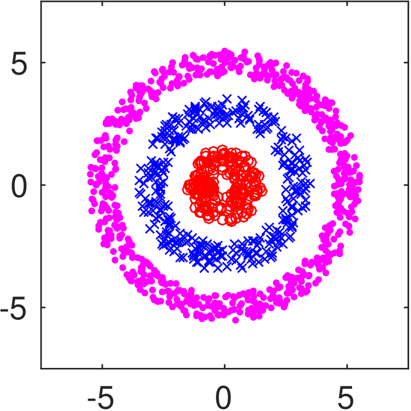
(a)

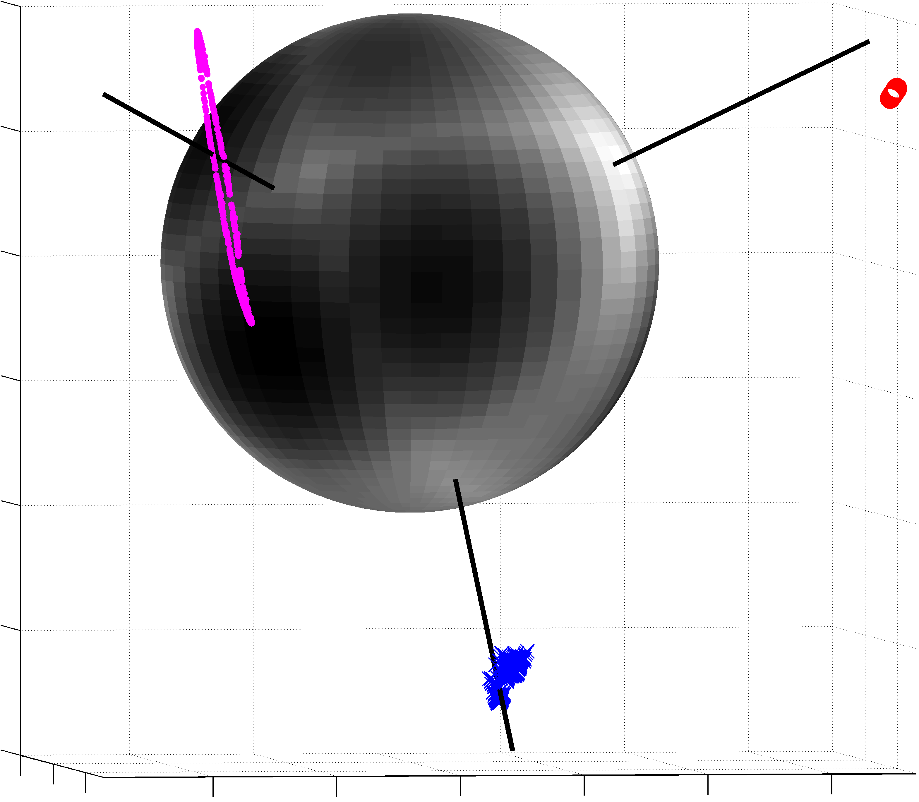
(b)

Figure 1: An illustration of spectral clustering on the concentric circle data. (a) The output of clustering. (b) The embedded data, the directional evaluations of $F_{g_{\mathrm{sig}}}$, and the recovered basis for clustering.

6.2 Image Segmentation Examples

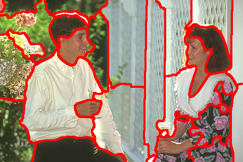
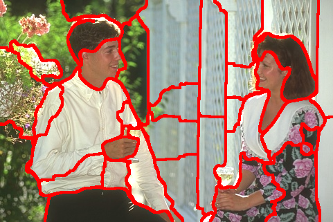
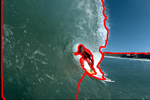
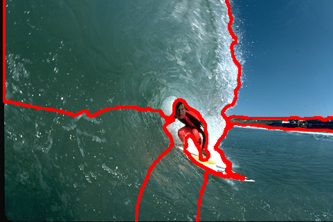
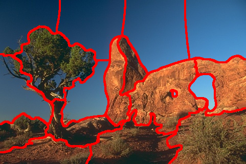
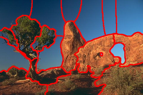
Figure 2: Segmented images. Segmentation using HBRopt-$g_{\mathrm{abs}}$ (left panels) compared to $k$-means (right panels). Red pixels mark the borders between segmented regions.

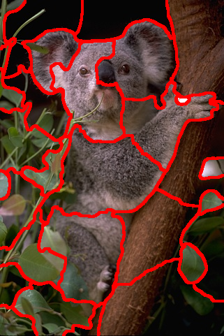
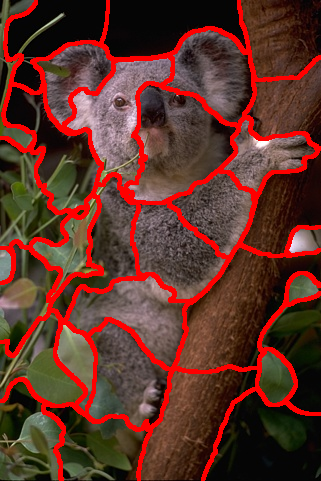
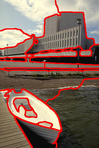
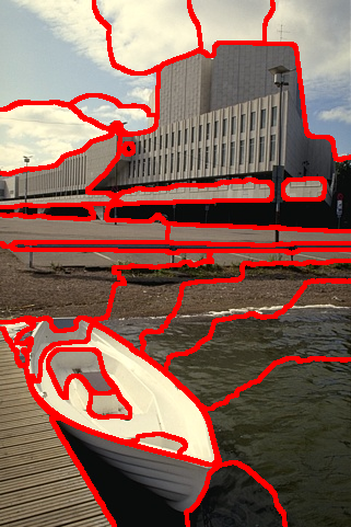
Figure 3: Segmented images. Segmentation using HBRopt-$g_{\mathrm{abs}}$ (left panels) compared to $k$-means (right panels). Red pixels mark the borders between segmented regions.

Spectral clustering was first applied to image segmentation by Shi and Malik [17], and it has remained a popular application of spectral clustering. The goal in image segmentation is to divide an image into regions which represent distinct objects or features of the image. Figure 2 and Figure 3 show several segmentations produced by HBRopt-$g_{\mathrm{abs}}$ and spherical $k$-means on several example images from the BSDS300 test set [13].

For this example application, we used a relatively simple notion of similarity based only on the color and proximity of the image’s pixels. Let $p_{i}$ denote the $i$^th pixel. Each $p_{i}$ has a location $\mathbf{x}_{i}$ and an RGB color $\mathbf{c}_{i}=(r_{i},g_{i},b_{i})^{T}$. We used the following similarity between any two distinct pixels $p_{i}$ and $p_{j}$:

$$a_{ij}=\begin{cases}e^{-\frac{1}{\alpha^{2}}\lVert\mathbf{x}_{i}-\mathbf{x}_{j}\rVert^{2}}e^{-\frac{1}{\beta^{2}}\lVert\mathbf{c}_{i}-\mathbf{c}_{j}\rVert^{2}}&\text{if $\lVert\mathbf{x}_{i}-\mathbf{x}_{j}\rVert<R$}\\ 0&\text{if $\lVert\mathbf{x}_{i}-\mathbf{x}_{j}\rVert\geq R$}\end{cases}$$ (6)

for some parameters $\alpha$, $\beta$, and radius $R$. By enforcing that $a_{ij}$ is 0 for points which are not too close, we build a sparse similarity matrix which greatly speeds up the computations. As the similarity measure decays exponentially with distance, the zeroed entries would be very small anyway.

Determining the number of clusters to use in spectral clustering is an unsolved problem. However, the BSDS300 data set includes hand labeled segmentations. From the hand labeled segmentations for a particular image, one human segmentation was chosen at random and the number of segments from that segmentation was used as the number of clusters $k$ for spectral clustering to search for. No other information from the human segmentations was used in generating the image segmentations.

In order to reduce the effect of salt and pepper type noise, the images were preprocessed using $9\times 9$ median filtering prior to constructing the similarity matrices. The similarity from equation (6) was constructed with common fixed values of $\alpha$, $\beta$, and $R$ across all images. Spectral clustering was performed using HBRopt under the contrast function $g_{\mathrm{abs}}$ and the $L_{\mathrm{rw}}$ embedding.

Qualitatively, we found that for the same embedding, $k$-means is more likely to over segment large regions within the image, in effect balancing the cluster sizes. In contrast, our proposed HBRopt algorithm tended to segment out additional small regions within the image more frequently.

6.3 Stochastic Block Model with Imbalanced Clusters

We construct a similarity graph $A=\operatorname{diag}(A_{1},A_{2},A_{3})+E$ where each $A_{i}$ is a symmetric matrix corresponding to a cluster and $E$ is a small perturbation. We set $A_{1}=A_{2}$ to be $10\times 10$ matrices with entries $0.1$. We set $A_{3}$ to be a $1000\times 1000$ matrix which is symmetric, approximately 95% sparse with randomly chosen non-zero locations set to 0.001. When performing this experiment $50$ times, HBRopt-$g_{sig}$ obtained a mean accuracy of 99.9%. In contrast, spherical $k$-means with randomly chosen starting points obtained a mean accuracy of only 42.1%. It turns out that splitting the large cluster is in fact optimal in terms of the spherical $k$-means objective function but leads to poor classification performance. Our method does not suffer from that shortcoming.

6.4 Performance Evaluation on UCI Datasets

	oracle-	$k$-means	HBRopt					HBRenum
	centroids	cosine	$g_{\mathrm{abs}}$	$g_{\mathrm{gau}}$	$g_{3}{\phantom{{}^{\prime}}}$	$g_{\mathrm{ht}}$	$g_{\mathrm{sig}}$	$g_{\mathrm{abs}}$	$g_{\mathrm{gau}}$	$g_{3}^{\phantom{{}^{\prime}}}$	$g_{\mathrm{ht}}$	$g_{\mathrm{sig}}$
E. coli	79.7	69.0	80.9	81.2	79.3	81.2	80.6	68.7	81.5	81.5	68.7	81.5
flags	33.2	33.1	36.8	34.1	36.6	36.8	34.4	34.7	36.8	36.8	34.7	36.8
glass	49.3	46.8	47.0	46.8	47.0	47.0	46.8	47.0	47.0	47.0	47.0	47.0
Iris	84.0	84.0	82.8	83.4	78.5	83.4	83.2	67.3	83.3	83.3	71.3	84.0
thyroid	72.4	80.4	82.4	81.3	82.2	82.2	81.5	81.8	82.2	82.2	81.8	82.2
car eval	56.1	36.4	37.0	36.3	36.3	35.2	36.6	49.6	32.3	41.1	49.9	41.1
cell cycle	74.2	62.7	64.3	64.4	63.8	64.5	64.0	60.1	62.9	64.8	61.1	62.7

Table 1: Percentage accuracy of spectral clustering algorithms, with the best performing non-oracle algorithm bolded.

We compare spectral clustering performance on a number of data sets with unbalanced cluster sizes. In particular, we use the E. coli, flags, glass, Iris, thyroid disease, and car evaluation data sets which are part of the UCI machine learning repository [3]. We also use the standardized gene expression data set [24, 23], which is also referred to as cell cycle. For the flags data set, we used religion as the ground truth labels, and for thyroid disease, we used the new-thyroid data.

For all data sets, we only used fields for which there were no missing values, we normalized the data such that every field had unit standard deviation, and we constructed the similarity matrix $A$ using a Gaussian kernel $k(\mathbf{y}_{i},\mathbf{y}_{j})=\exp(-\alpha\lVert\mathbf{y}_{i}-\mathbf{y}_{j}\rVert^{2})$. The parameter $\alpha$ was chosen separately for each data set in order to create a good embedding. The choices of $\alpha$ were: 0.25 for E. coli, 32 for glass, 0.5 for Iris, 32 for thyroid disease, 128 for flags, 0.25 for car evaluation, and 0.125 for cell cycle.

The spectral embedding was performed using the symmetric normalized Laplacian $L_{\mathrm{sym}}$. Then, the clustering performance of our proposed algorithms HBRopt and HBRenum (implemented with $\delta=3\pi/8$ radians) were compared with the following baselines:

• oracle-centroids: The means $\mu_{j}=\frac{1}{{|\mathcal{S}_{j}|}}\sum_{i\in\mathcal{S}_{j}}\frac{x_{i\mathchoice{{\hbox to3.61108pt{\hss\leavevmode\hbox{\raisebox{0.0pt}{\scalebox{0.5}{\raisebox{0.0pt}{$\displaystyle\bullet$}}}}\hss}}}{{\hbox to3.61108pt{\hss\leavevmode\hbox{\raisebox{0.0pt}{\scalebox{0.5}{\raisebox{0.0pt}{$\textstyle\bullet$}}}}\hss}}}{{\hbox to2.86108pt{\hss\leavevmode\hbox{\raisebox{0.0pt}{\scalebox{0.5}{\raisebox{0.0pt}{$\scriptstyle\bullet$}}}}\hss}}}{{\hbox to2.36108pt{\hss\leavevmode\hbox{\raisebox{0.0pt}{\scalebox{0.5}{\raisebox{0.0pt}{$\scriptscriptstyle\bullet$}}}}\hss}}}}}{\lVert x_{i\mathchoice{{\hbox to3.61108pt{\hss\leavevmode\hbox{\raisebox{0.0pt}{\scalebox{0.5}{\raisebox{0.0pt}{$\displaystyle\bullet$}}}}\hss}}}{{\hbox to3.61108pt{\hss\leavevmode\hbox{\raisebox{0.0pt}{\scalebox{0.5}{\raisebox{0.0pt}{$\textstyle\bullet$}}}}\hss}}}{{\hbox to2.86108pt{\hss\leavevmode\hbox{\raisebox{0.0pt}{\scalebox{0.5}{\raisebox{0.0pt}{$\scriptstyle\bullet$}}}}\hss}}}{{\hbox to2.36108pt{\hss\leavevmode\hbox{\raisebox{0.0pt}{\scalebox{0.5}{\raisebox{0.0pt}{$\scriptscriptstyle\bullet$}}}}\hss}}}}\rVert}$ are set using the ground truth labels for all $j\in[k]$. Points are assigned to their nearest cluster mean in cosine distance.

• $k$-means-cosine: Spherical $k$-means (standard matlab kmeans library function called using the cosine distance and using the default $k$-means++ mean initialization) is run with a random initialization of the means, (cf. [15]).

We report the clustering accuracy of each algorithm in Table 1. The accuracy is computed using the best matching between the clusters and the true labels. The reported results consist of the mean performance over a set of 25 runs for each algorithm. The number of clusters being searched for was set to the ground truth number of clusters. In most cases, our proposed algorithms show improvement in performance over spherical $k$-means.

7 Basis Recovery With Each Laplacian Embedding

We have already argued that graph Laplacians $L$ and $L_{\mathrm{rw}}$ can be used for spectral clustering within our BEF framework, and we have asserted that $L_{\mathrm{sym}}$ can also be used. We now discuss how orthogonal BEF recovery can be used for spectral clustering in the setting where $G$ consists of $k$ connected components using any of the graph Laplacians. First, in section 7.1, we show how the Laplacian embedding for the symmetric normalized Laplacian $L_{\mathrm{sym}}$ differs and generalizes upon the embedding structure arising for $L$ and $L_{\mathrm{rw}}$ (cf. Proposition 7). Then, in section 7.2, we prove that the spectral embedding induced by any of the discussed graph Laplacians gives rise to an optimization problem on $\mathbb{S}^{k-1}$ in which the local maxima enumerate the desired clusters for spectral clustering. More precisely, we prove a generalization of Theorem 9 which includes embeddings generated using $L$, $L_{\mathrm{rw}}$, and $L_{\mathrm{sym}}$.

The discussion in this section highlights the differences between using $L_{\mathrm{sym}}$ and using either $L$ or $L_{\mathrm{rw}}$ for the proposed spectral algorithms. Whereas taking an orthogonal basis of $\mathcal{N}(L)$ or $\mathcal{N}(L_{\mathrm{rw}})$ produces embedded points which are orthogonal and of fixed norm within any particular class, using $\mathcal{N}(L_{\mathrm{sym}})$ produces embedded points along perpendicular rays but with varying intra-class norms as will be seen in Proposition 10. Despite these differences, when given a contrast function $g$ meeting the strict convexity criterion from Assumption 3, the proposed algorithms HBRopt and HBRenum which worked for spectral clustering using $L$ and $L_{\mathrm{rw}}$ also work for spectral clustering using $L_{\mathrm{sym}}$.

7.1 Null Space Structure of the Normalized Laplacians

We now investigate the null space structure of the normalized graph Laplacians. We will first describe the null space structures $L_{\mathrm{sym}}$ and $L_{\mathrm{rw}}$ for a graph $G$ consisting of $k$ components. Then, we will show how the null space structures of $L_{\mathrm{sym}}$, $L_{\mathrm{rw}}$, and $L$ can all be viewed within a single, more generalized notion of a graph embedding.

Let $G=(V,A)$ be an $n$-vertex graph containing $k$ connected components such that the $i$^th component has vertices with indices in the set $\mathcal{S}_{i}$. For any set $C\subset V$, we define

$$\delta_{\mathfrak{D}}(C):=\sum_{i\in C}\mathfrak{d}_{ii}\ .$$ (7)

where $\mathfrak{D}=\operatorname{diag}(\mathfrak{d}_{11},\mathfrak{d}_{22},\dotsc,\mathfrak{d}_{nn})$ is a diagonal matrix with strictly positive entries. For now, we will take $\mathfrak{D}$ to be the diagonal degree matrix $D$ such that $\mathfrak{d}_{ii}=d_{ii}=\sum_{j=1}^{n}a_{ij}$. Then, $\delta_{D}(C)$ is the sum of vertex degrees for vertices in the set $C$. Using this definition, we are able to characterize the embedding structure of $L_{\mathrm{sym}}$.

Proposition 10.

Let $G$ be a similarity graph consisting of $k$ connected components for which $L_{\mathrm{sym}}$ is well defined. Let the vertex indices be partitioned into sets $\mathcal{S}_{1},\dotsc,\mathcal{S}_{k}$ corresponding to the $k$ connected components. Then, $\operatorname{dim}(\mathcal{N}(L_{\mathrm{sym}}))=k$. If $X=(x_{\mathchoice{{\hbox to5.05554pt{\hss\leavevmode\hbox{\raisebox{0.0pt}{\scalebox{0.5}{\raisebox{0.0pt}{$\displaystyle\bullet$}}}}\hss}}}{{\hbox to5.05554pt{\hss\leavevmode\hbox{\raisebox{0.0pt}{\scalebox{0.5}{\raisebox{0.0pt}{$\textstyle\bullet$}}}}\hss}}}{{\hbox to4.00554pt{\hss\leavevmode\hbox{\raisebox{0.0pt}{\scalebox{0.5}{\raisebox{0.0pt}{$\scriptstyle\bullet$}}}}\hss}}}{{\hbox to3.30554pt{\hss\leavevmode\hbox{\raisebox{0.0pt}{\scalebox{0.5}{\raisebox{0.0pt}{$\scriptscriptstyle\bullet$}}}}\hss}}}1},\dotsc,x_{\mathchoice{{\hbox to5.05554pt{\hss\leavevmode\hbox{\raisebox{0.0pt}{\scalebox{0.5}{\raisebox{0.0pt}{$\displaystyle\bullet$}}}}\hss}}}{{\hbox to5.05554pt{\hss\leavevmode\hbox{\raisebox{0.0pt}{\scalebox{0.5}{\raisebox{0.0pt}{$\textstyle\bullet$}}}}\hss}}}{{\hbox to4.00554pt{\hss\leavevmode\hbox{\raisebox{0.0pt}{\scalebox{0.5}{\raisebox{0.0pt}{$\scriptstyle\bullet$}}}}\hss}}}{{\hbox to3.30554pt{\hss\leavevmode\hbox{\raisebox{0.0pt}{\scalebox{0.5}{\raisebox{0.0pt}{$\scriptscriptstyle\bullet$}}}}\hss}}}k})$ contains a scaled basis of $\mathcal{N}(L_{\mathrm{sym}})$ in its columns such that $\lVert x_{\mathchoice{{\hbox to5.05554pt{\hss\leavevmode\hbox{\raisebox{0.0pt}{\scalebox{0.5}{\raisebox{0.0pt}{$\displaystyle\bullet$}}}}\hss}}}{{\hbox to5.05554pt{\hss\leavevmode\hbox{\raisebox{0.0pt}{\scalebox{0.5}{\raisebox{0.0pt}{$\textstyle\bullet$}}}}\hss}}}{{\hbox to4.00554pt{\hss\leavevmode\hbox{\raisebox{0.0pt}{\scalebox{0.5}{\raisebox{0.0pt}{$\scriptstyle\bullet$}}}}\hss}}}{{\hbox to3.30554pt{\hss\leavevmode\hbox{\raisebox{0.0pt}{\scalebox{0.5}{\raisebox{0.0pt}{$\scriptscriptstyle\bullet$}}}}\hss}}}i}\rVert=\sqrt{}n$, then there exist $k$ mutually orthogonal unit vectors $\mathbf{z}_{1},\dotsc,\mathbf{z}_{k}$ such that whenever $i\in\mathcal{S}_{j}$, the row vector

$$x_{i\mathchoice{{\hbox to5.05554pt{\hss\leavevmode\hbox{\raisebox{0.0pt}{\scalebox{0.5}{\raisebox{0.0pt}{$\displaystyle\bullet$}}}}\hss}}}{{\hbox to5.05554pt{\hss\leavevmode\hbox{\raisebox{0.0pt}{\scalebox{0.5}{\raisebox{0.0pt}{$\textstyle\bullet$}}}}\hss}}}{{\hbox to4.00554pt{\hss\leavevmode\hbox{\raisebox{0.0pt}{\scalebox{0.5}{\raisebox{0.0pt}{$\scriptstyle\bullet$}}}}\hss}}}{{\hbox to3.30554pt{\hss\leavevmode\hbox{\raisebox{0.0pt}{\scalebox{0.5}{\raisebox{0.0pt}{$\scriptscriptstyle\bullet$}}}}\hss}}}}=\sqrt{nd_{ii}\delta_{D}(\mathcal{S}_{j})^{-1}}\mathbf{z}_{j}^{T}\ .$$ (8)

Proof.

An important property of the symmetric normalized Laplacian [19, Proposition 3] is that for all $\mathbf{u}\in\mathbb{R}^{n}$,

$$\mathbf{u}^{T}L_{\mathrm{sym}}\mathbf{u}=\frac{1}{2}\sum_{i,j\in V}a_{ij}\left(\frac{u_{i}}{d_{ii}^{1/2}}-\frac{u_{j}}{d_{jj}^{1/2}}\right)^{2}\ .$$ (9)

$L_{\mathrm{sym}}$ is positive semi-definite, and $\mathbf{u}$ is a 0-eigenvector of $L_{\mathrm{sym}}$ if and only if plugging $\mathbf{u}$ into equation (9) yields 0. Let $\mathbf{y}_{\mathcal{S}_{j}}^{\phantom{*}}$ be the vector such that

$$\mathbf{y}_{\mathcal{S}_{j}}^{\phantom{*}}=\left\{\begin{array}[]{ll}d_{ii}^{1/2}&\text{if $i\in\mathcal{S}_{j}$.}\\ 0&\text{otherwise}\end{array}\right.\ .$$ (10)

Then, $B=(\delta_{D}(\mathcal{S}_{1})^{-1/2}\mathbf{y}_{\mathcal{S}_{1}}^{\phantom{*}},\dotsc,\delta_{D}(\mathcal{S}_{d})^{-1/2}\mathbf{y}_{\mathcal{S}_{d}}^{\phantom{*}})$ contains an orthonormal basis for $\mathcal{N}(L_{\mathrm{sym}})$ in its columns.

Defining $M_{\mathcal{S}_{i}}=\mathbf{y}_{\mathcal{S}_{i}}^{\phantom{*}}\mathbf{y}_{\mathcal{S}_{i}}^{T}$, we get:

$$P_{\mathcal{N}(L)}=BB^{T}=\sum_{i=1}^{k}\delta_{D}(\mathcal{S}_{i})^{-1}M_{\mathcal{S}_{i}}\ .$$ (11)

But $P_{\mathcal{N}(L_{\mathrm{sym}})}$ can be constructed from any orthonormal basis of $\mathcal{N}(L_{\mathrm{sym}})$. In particular, $P_{\mathcal{N}(L_{\mathrm{sym}})}=\frac{1}{n}XX^{T}$ as well. Hence, $\frac{1}{n}x_{i\mathchoice{{\hbox to5.05554pt{\hss\leavevmode\hbox{\raisebox{0.0pt}{\scalebox{0.5}{\raisebox{0.0pt}{$\displaystyle\bullet$}}}}\hss}}}{{\hbox to5.05554pt{\hss\leavevmode\hbox{\raisebox{0.0pt}{\scalebox{0.5}{\raisebox{0.0pt}{$\textstyle\bullet$}}}}\hss}}}{{\hbox to4.00554pt{\hss\leavevmode\hbox{\raisebox{0.0pt}{\scalebox{0.5}{\raisebox{0.0pt}{$\scriptstyle\bullet$}}}}\hss}}}{{\hbox to3.30554pt{\hss\leavevmode\hbox{\raisebox{0.0pt}{\scalebox{0.5}{\raisebox{0.0pt}{$\scriptscriptstyle\bullet$}}}}\hss}}}}\mathbin{\mathchoice{{\hbox to7.22218pt{\hss\leavevmode\hbox{\raisebox{0.0pt}{\scalebox{0.5}{\raisebox{0.0pt}{$\displaystyle\bullet$}}}}\hss}}}{{\hbox to7.22218pt{\hss\leavevmode\hbox{\raisebox{0.0pt}{\scalebox{0.5}{\raisebox{0.0pt}{$\textstyle\bullet$}}}}\hss}}}{{\hbox to5.72217pt{\hss\leavevmode\hbox{\raisebox{0.0pt}{\scalebox{0.5}{\raisebox{0.0pt}{$\scriptstyle\bullet$}}}}\hss}}}{{\hbox to4.72217pt{\hss\leavevmode\hbox{\raisebox{0.0pt}{\scalebox{0.5}{\raisebox{0.0pt}{$\scriptscriptstyle\bullet$}}}}\hss}}}}x_{j\mathchoice{{\hbox to5.05554pt{\hss\leavevmode\hbox{\raisebox{0.0pt}{\scalebox{0.5}{\raisebox{0.0pt}{$\displaystyle\bullet$}}}}\hss}}}{{\hbox to5.05554pt{\hss\leavevmode\hbox{\raisebox{0.0pt}{\scalebox{0.5}{\raisebox{0.0pt}{$\textstyle\bullet$}}}}\hss}}}{{\hbox to4.00554pt{\hss\leavevmode\hbox{\raisebox{0.0pt}{\scalebox{0.5}{\raisebox{0.0pt}{$\scriptstyle\bullet$}}}}\hss}}}{{\hbox to3.30554pt{\hss\leavevmode\hbox{\raisebox{0.0pt}{\scalebox{0.5}{\raisebox{0.0pt}{$\scriptscriptstyle\bullet$}}}}\hss}}}}=(P_{\mathcal{N}(L)})_{ij}=\delta_{D}(\mathcal{S}_{\ell})^{-1}d_{ii}^{1/2}d_{jj}^{1/2}$ precisely when there exists $\ell\in[k]$ such that $i,j\in\mathcal{S}_{\ell}$. Otherwise, $x_{i\mathchoice{{\hbox to5.05554pt{\hss\leavevmode\hbox{\raisebox{0.0pt}{\scalebox{0.5}{\raisebox{0.0pt}{$\displaystyle\bullet$}}}}\hss}}}{{\hbox to5.05554pt{\hss\leavevmode\hbox{\raisebox{0.0pt}{\scalebox{0.5}{\raisebox{0.0pt}{$\textstyle\bullet$}}}}\hss}}}{{\hbox to4.00554pt{\hss\leavevmode\hbox{\raisebox{0.0pt}{\scalebox{0.5}{\raisebox{0.0pt}{$\scriptstyle\bullet$}}}}\hss}}}{{\hbox to3.30554pt{\hss\leavevmode\hbox{\raisebox{0.0pt}{\scalebox{0.5}{\raisebox{0.0pt}{$\scriptscriptstyle\bullet$}}}}\hss}}}}\perp x_{j\mathchoice{{\hbox to5.05554pt{\hss\leavevmode\hbox{\raisebox{0.0pt}{\scalebox{0.5}{\raisebox{0.0pt}{$\displaystyle\bullet$}}}}\hss}}}{{\hbox to5.05554pt{\hss\leavevmode\hbox{\raisebox{0.0pt}{\scalebox{0.5}{\raisebox{0.0pt}{$\textstyle\bullet$}}}}\hss}}}{{\hbox to4.00554pt{\hss\leavevmode\hbox{\raisebox{0.0pt}{\scalebox{0.5}{\raisebox{0.0pt}{$\scriptstyle\bullet$}}}}\hss}}}{{\hbox to3.30554pt{\hss\leavevmode\hbox{\raisebox{0.0pt}{\scalebox{0.5}{\raisebox{0.0pt}{$\scriptscriptstyle\bullet$}}}}\hss}}}}$.

Note that for $i,j\in\mathcal{S}_{\ell}$,

$$\cos(\angle(x_{i\mathchoice{{\hbox to5.05554pt{\hss\leavevmode\hbox{\raisebox{0.0pt}{\scalebox{0.5}{\raisebox{0.0pt}{$\displaystyle\bullet$}}}}\hss}}}{{\hbox to5.05554pt{\hss\leavevmode\hbox{\raisebox{0.0pt}{\scalebox{0.5}{\raisebox{0.0pt}{$\textstyle\bullet$}}}}\hss}}}{{\hbox to4.00554pt{\hss\leavevmode\hbox{\raisebox{0.0pt}{\scalebox{0.5}{\raisebox{0.0pt}{$\scriptstyle\bullet$}}}}\hss}}}{{\hbox to3.30554pt{\hss\leavevmode\hbox{\raisebox{0.0pt}{\scalebox{0.5}{\raisebox{0.0pt}{$\scriptscriptstyle\bullet$}}}}\hss}}}},x_{j,\mathchoice{{\hbox to5.05554pt{\hss\leavevmode\hbox{\raisebox{0.0pt}{\scalebox{0.5}{\raisebox{0.0pt}{$\displaystyle\bullet$}}}}\hss}}}{{\hbox to5.05554pt{\hss\leavevmode\hbox{\raisebox{0.0pt}{\scalebox{0.5}{\raisebox{0.0pt}{$\textstyle\bullet$}}}}\hss}}}{{\hbox to4.00554pt{\hss\leavevmode\hbox{\raisebox{0.0pt}{\scalebox{0.5}{\raisebox{0.0pt}{$\scriptstyle\bullet$}}}}\hss}}}{{\hbox to3.30554pt{\hss\leavevmode\hbox{\raisebox{0.0pt}{\scalebox{0.5}{\raisebox{0.0pt}{$\scriptscriptstyle\bullet$}}}}\hss}}}}))=\frac{x_{i\mathchoice{{\hbox to5.05554pt{\hss\leavevmode\hbox{\raisebox{0.0pt}{\scalebox{0.5}{\raisebox{0.0pt}{$\displaystyle\bullet$}}}}\hss}}}{{\hbox to5.05554pt{\hss\leavevmode\hbox{\raisebox{0.0pt}{\scalebox{0.5}{\raisebox{0.0pt}{$\textstyle\bullet$}}}}\hss}}}{{\hbox to4.00554pt{\hss\leavevmode\hbox{\raisebox{0.0pt}{\scalebox{0.5}{\raisebox{0.0pt}{$\scriptstyle\bullet$}}}}\hss}}}{{\hbox to3.30554pt{\hss\leavevmode\hbox{\raisebox{0.0pt}{\scalebox{0.5}{\raisebox{0.0pt}{$\scriptscriptstyle\bullet$}}}}\hss}}}}\mathbin{\mathchoice{{\hbox to7.22218pt{\hss\leavevmode\hbox{\raisebox{0.0pt}{\scalebox{0.5}{\raisebox{0.0pt}{$\displaystyle\bullet$}}}}\hss}}}{{\hbox to7.22218pt{\hss\leavevmode\hbox{\raisebox{0.0pt}{\scalebox{0.5}{\raisebox{0.0pt}{$\textstyle\bullet$}}}}\hss}}}{{\hbox to5.72217pt{\hss\leavevmode\hbox{\raisebox{0.0pt}{\scalebox{0.5}{\raisebox{0.0pt}{$\scriptstyle\bullet$}}}}\hss}}}{{\hbox to4.72217pt{\hss\leavevmode\hbox{\raisebox{0.0pt}{\scalebox{0.5}{\raisebox{0.0pt}{$\scriptscriptstyle\bullet$}}}}\hss}}}}x_{j\mathchoice{{\hbox to5.05554pt{\hss\leavevmode\hbox{\raisebox{0.0pt}{\scalebox{0.5}{\raisebox{0.0pt}{$\displaystyle\bullet$}}}}\hss}}}{{\hbox to5.05554pt{\hss\leavevmode\hbox{\raisebox{0.0pt}{\scalebox{0.5}{\raisebox{0.0pt}{$\textstyle\bullet$}}}}\hss}}}{{\hbox to4.00554pt{\hss\leavevmode\hbox{\raisebox{0.0pt}{\scalebox{0.5}{\raisebox{0.0pt}{$\scriptstyle\bullet$}}}}\hss}}}{{\hbox to3.30554pt{\hss\leavevmode\hbox{\raisebox{0.0pt}{\scalebox{0.5}{\raisebox{0.0pt}{$\scriptscriptstyle\bullet$}}}}\hss}}}}}{\lVert x_{i\mathchoice{{\hbox to5.05554pt{\hss\leavevmode\hbox{\raisebox{0.0pt}{\scalebox{0.5}{\raisebox{0.0pt}{$\displaystyle\bullet$}}}}\hss}}}{{\hbox to5.05554pt{\hss\leavevmode\hbox{\raisebox{0.0pt}{\scalebox{0.5}{\raisebox{0.0pt}{$\textstyle\bullet$}}}}\hss}}}{{\hbox to4.00554pt{\hss\leavevmode\hbox{\raisebox{0.0pt}{\scalebox{0.5}{\raisebox{0.0pt}{$\scriptstyle\bullet$}}}}\hss}}}{{\hbox to3.30554pt{\hss\leavevmode\hbox{\raisebox{0.0pt}{\scalebox{0.5}{\raisebox{0.0pt}{$\scriptscriptstyle\bullet$}}}}\hss}}}}\rVert\lVert x_{j\mathchoice{{\hbox to5.05554pt{\hss\leavevmode\hbox{\raisebox{0.0pt}{\scalebox{0.5}{\raisebox{0.0pt}{$\displaystyle\bullet$}}}}\hss}}}{{\hbox to5.05554pt{\hss\leavevmode\hbox{\raisebox{0.0pt}{\scalebox{0.5}{\raisebox{0.0pt}{$\textstyle\bullet$}}}}\hss}}}{{\hbox to4.00554pt{\hss\leavevmode\hbox{\raisebox{0.0pt}{\scalebox{0.5}{\raisebox{0.0pt}{$\scriptstyle\bullet$}}}}\hss}}}{{\hbox to3.30554pt{\hss\leavevmode\hbox{\raisebox{0.0pt}{\scalebox{0.5}{\raisebox{0.0pt}{$\scriptscriptstyle\bullet$}}}}\hss}}}}\rVert}$$

$$\quad=\frac{n\delta_{D}(\mathcal{S}_{\ell})^{-1}_{\phantom{*}}d_{ii}^{1/2}d_{jj}^{1/2}}{(n^{1/2}\delta_{D}(\mathcal{S}_{\ell})^{-1/2}_{\phantom{*}}d_{ii}^{1/2})(n^{1/2}_{\phantom{*}}\delta_{D}(\mathcal{S}_{\ell})^{-1/2}_{\phantom{*}}d_{jj}^{1/2})}=1\ .$$

Thus, points from the same cluster lie on the same ray from the origin. It follows that there are $k$ mutually orthogonal unit vectors, $\mathbf{z}_{1},\dotsc,\mathbf{z}_{k}$ such that $x_{i\mathchoice{{\hbox to5.05554pt{\hss\leavevmode\hbox{\raisebox{0.0pt}{\scalebox{0.5}{\raisebox{0.0pt}{$\displaystyle\bullet$}}}}\hss}}}{{\hbox to5.05554pt{\hss\leavevmode\hbox{\raisebox{0.0pt}{\scalebox{0.5}{\raisebox{0.0pt}{$\textstyle\bullet$}}}}\hss}}}{{\hbox to4.00554pt{\hss\leavevmode\hbox{\raisebox{0.0pt}{\scalebox{0.5}{\raisebox{0.0pt}{$\scriptstyle\bullet$}}}}\hss}}}{{\hbox to3.30554pt{\hss\leavevmode\hbox{\raisebox{0.0pt}{\scalebox{0.5}{\raisebox{0.0pt}{$\scriptscriptstyle\bullet$}}}}\hss}}}}=\sqrt{nd_{ii}\delta_{D}(\mathcal{S}_{\ell})^{-1}}\mathbf{z}_{\ell}^{T}$ for each $i\in\mathcal{S}_{\ell}$. ∎

We will make use of the close connection between the eigenvector structure of $L_{\mathrm{rw}}$ and $L_{\mathrm{sym}}$ in order to characterize the Laplacian embedding structure of $L_{\mathrm{rw}}$. The following fact can be found in the tutorial [19, Proposition 3].

Fact 11.

$(\lambda,\mathbf{u})$ is an eigenvalue-eigenvector pair of $L_{\mathrm{rw}}$ if and only if $(\lambda,D^{1/2}\mathbf{u})$ is an eigenvalue-eigenvector pair for $L_{\mathrm{sym}}$.

By using Fact 11 and Proposition 10, we obtain the embedding structure for $L_{rw}$.

Proposition 12.

Let the similarity graph $G=(V,A)$ contain $k$ connected components with indices in the sets $\mathcal{S}_{1},\dotsc,\mathcal{S}_{k}$, let $n={|V|}$, and let $L_{\mathrm{rw}}$ be well defined for $G$. Then, $\mathcal{N}(L_{\mathrm{rw}})$ has dimensionality $k$. Let $X=(x_{\mathchoice{{\hbox to5.05554pt{\hss\leavevmode\hbox{\raisebox{0.0pt}{\scalebox{0.5}{\raisebox{0.0pt}{$\displaystyle\bullet$}}}}\hss}}}{{\hbox to5.05554pt{\hss\leavevmode\hbox{\raisebox{0.0pt}{\scalebox{0.5}{\raisebox{0.0pt}{$\textstyle\bullet$}}}}\hss}}}{{\hbox to4.00554pt{\hss\leavevmode\hbox{\raisebox{0.0pt}{\scalebox{0.5}{\raisebox{0.0pt}{$\scriptstyle\bullet$}}}}\hss}}}{{\hbox to3.30554pt{\hss\leavevmode\hbox{\raisebox{0.0pt}{\scalebox{0.5}{\raisebox{0.0pt}{$\scriptscriptstyle\bullet$}}}}\hss}}}1},\dotsc,x_{\mathchoice{{\hbox to5.05554pt{\hss\leavevmode\hbox{\raisebox{0.0pt}{\scalebox{0.5}{\raisebox{0.0pt}{$\displaystyle\bullet$}}}}\hss}}}{{\hbox to5.05554pt{\hss\leavevmode\hbox{\raisebox{0.0pt}{\scalebox{0.5}{\raisebox{0.0pt}{$\textstyle\bullet$}}}}\hss}}}{{\hbox to4.00554pt{\hss\leavevmode\hbox{\raisebox{0.0pt}{\scalebox{0.5}{\raisebox{0.0pt}{$\scriptstyle\bullet$}}}}\hss}}}{{\hbox to3.30554pt{\hss\leavevmode\hbox{\raisebox{0.0pt}{\scalebox{0.5}{\raisebox{0.0pt}{$\scriptscriptstyle\bullet$}}}}\hss}}}k})$ contain $k$ scaled, orthogonal column vectors forming a basis of $\mathcal{N}(L_{\mathrm{rw}})$ such that $\lVert x_{\mathchoice{{\hbox to5.05554pt{\hss\leavevmode\hbox{\raisebox{0.0pt}{\scalebox{0.5}{\raisebox{0.0pt}{$\displaystyle\bullet$}}}}\hss}}}{{\hbox to5.05554pt{\hss\leavevmode\hbox{\raisebox{0.0pt}{\scalebox{0.5}{\raisebox{0.0pt}{$\textstyle\bullet$}}}}\hss}}}{{\hbox to4.00554pt{\hss\leavevmode\hbox{\raisebox{0.0pt}{\scalebox{0.5}{\raisebox{0.0pt}{$\scriptstyle\bullet$}}}}\hss}}}{{\hbox to3.30554pt{\hss\leavevmode\hbox{\raisebox{0.0pt}{\scalebox{0.5}{\raisebox{0.0pt}{$\scriptscriptstyle\bullet$}}}}\hss}}}j}\rVert=\sqrt{}n$ for each $j\in[k]$. Then, there exist weights $w_{1},\dotsc,w_{k}$ with $w_{j}=\frac{{|\mathcal{S}_{j}|}}{n}$ and mutually orthogonal vectors $\mathbf{z}_{1},\dotsc,\mathbf{z}_{k}\in\mathbb{R}^{k}$ such that whenever $i\in\mathcal{S}_{j}$, the row vector $x_{i\mathchoice{{\hbox to5.05554pt{\hss\leavevmode\hbox{\raisebox{0.0pt}{\scalebox{0.5}{\raisebox{0.0pt}{$\displaystyle\bullet$}}}}\hss}}}{{\hbox to5.05554pt{\hss\leavevmode\hbox{\raisebox{0.0pt}{\scalebox{0.5}{\raisebox{0.0pt}{$\textstyle\bullet$}}}}\hss}}}{{\hbox to4.00554pt{\hss\leavevmode\hbox{\raisebox{0.0pt}{\scalebox{0.5}{\raisebox{0.0pt}{$\scriptstyle\bullet$}}}}\hss}}}{{\hbox to3.30554pt{\hss\leavevmode\hbox{\raisebox{0.0pt}{\scalebox{0.5}{\raisebox{0.0pt}{$\scriptscriptstyle\bullet$}}}}\hss}}}}=\frac{1}{\sqrt{w_{j}}}\mathbf{z}_{j}^{T}$.

Proof.

By Fact 11, we may construct an orthogonal basis of $\mathcal{N}(L_{\mathrm{rw}})$ using a particular choice of orthogonal basis of $\mathcal{N}(L_{\mathrm{sym}})$. In particular, we define the vectors $\mathbf{y}_{\SS_{j}}$ the same as in the proof of Proposition 10, and we obtain that the vectors $\tilde{\mathbf{y}}_{\SS_{j}}^{\phantom{*}}:=D^{-1/2}\mathbf{y}_{\SS_{j}}^{\phantom{*}}$ are $0$-eigenvectors of $L_{\mathrm{rw}}$. Using equation (10), we see that $\mathbf{y}_{\SS_{j}}^{\phantom{*}}=\mathbf{1}_{\SS_{j}}$. In particular, it follows that $\{{|\SS_{1}|}^{-1/2}\mathbf{1}_{\SS_{1}},\dotsc,{|\SS_{k}|}^{-1/2}\mathbf{1}_{\SS_{k}}\}$ is an orthonormal basis of $\mathcal{N}(L_{\mathrm{rw}})$. From the discussion around equation (3), it follows that $\mathcal{N}(L)$ and $\mathcal{N}(L_{\mathrm{rw}})$ are the same space in this setting where $G$ consists of $k$ connected components. Our desired result thus follows from Proposition 7. ∎

We note that the Propositions 7, 10, and 12 are closely. From Propositions 7 and 12, we see that $L$ and $L_{\mathrm{rw}}$ give rise to the same embedding structure when $G$ consists of $k$ connected components. Further, we may place the embedding structure for $L$ (or equivalently $L_{\mathrm{rw}}$) into the notation used for describing the ray structure of $L_{\mathrm{sym}}$. In particular, if we let $\mathfrak{D}=\mathcal{I}$, we see that $\delta_{\mathcal{I}}(\SS_{j})={|\SS_{j}|}$. Recalling that $w_{j}=\frac{{|\SS_{j}|}}{n}$, we see (by replacing $D$ with $\mathcal{I}$ in equation (8)) that $\sqrt{n\mathcal{I}_{ii}\delta_{\mathcal{I}}(\SS_{j})^{-1}}\mathbf{z}_{j}^{T}=\frac{1}{\sqrt{w_{j}}}\mathbf{z}_{j}^{T}$, which is the required replacement to recreate the statements of Proposition 7 and Proposition 12. In particular, we may create a generalized notion of a graph embedding which captures all of the Laplacian embeddings.

Definition 13.

Let $G$ be a similarity graph consisting of $n$ vertices and $k$ connected components such indices partitioned into sets $\SS_{1},\dotsc,\SS_{k}$ corresponding to the connected components. Let $\mathfrak{D}=\operatorname{diag}(\mathfrak{d}_{11},\dotsc,\mathfrak{d}_{nn})$ be a positive definite matrix. Let $\varphi$ be a map which takes the $i$^th vertex of $G$ to a point $\mathbf{x}_{i}\in\mathbb{R}^{k}$. If there exists an orthonormal basis $\mathbf{z}_{1},\dotsc,\mathbf{z}_{k}$ of $\mathbb{R}^{k}$ such that $\mathbf{x}_{i}=\sqrt{n\mathfrak{d}_{ii}\delta_{\mathfrak{D}}(\SS_{j})^{-1}}\mathbf{z}_{j}$ for each $i\in\SS_{j}$, then we call $\varphi$ a ($G$, $\mathfrak{D}$)-orthogonal embedding.

We see by Proposition 10, the Laplacian embedding induced by $L_{\mathrm{sym}}$ is a $(G,D)$-orthogonal embedding; and by Propositions 7 and 12, the Laplacian embedding induced by $L$ and $L_{\mathrm{rw}}$ are $(G,\mathcal{I})$-orthogonal embedding.

7.2 Maxima Structure of the Resulting BEFs

In this section, we demonstrate that by performing function maximization over the directional projections of embedded data arising from any of the Laplacian embeddings, we are able to recover the desired clusters for spectral clustering. We will make use of the following construction.

Construction 14.

Let $G$ be a similarity graph consisting of $n$ vertices and $k$ connected components with indices partitioned into the sets $\SS_{1},\dotsc,\SS_{k}$. We suppose that $\mathfrak{D}=\operatorname{diag}(\mathfrak{d}_{11},\dotsc,\mathfrak{d}_{nn})$ is a positive definite matrix. We suppose that $\mathbf{x}_{1},\dotsc,\mathbf{x}_{n}$ is a $(G,\mathfrak{D})$-orthogonal embedding of the vertices of $G$ such that $\mathbf{x}_{i}=\sqrt{n\mathfrak{d}_{ii}\delta_{\mathfrak{D}}(\SS_{j})^{-1}}\mathbf{z}_{j}$ for each $i$ in $\SS_{j}$. Parallel to the text of section 5, we construct a function $F_{g}:\mathbb{S}^{k-1}\rightarrow\mathbb{R}$ from a continuous contrast function $g:[0,\infty)\rightarrow\mathbb{R}$ where it is assumed that $t\mapsto g(\sqrt{t})$ is strictly convex (cf. Assumption 3). We construct $F_{g}$ as

$$F_{g}(\mathbf{u}) :=\frac{1}{n}\sum_{i=1}^{n}g({|\mathbf{u}\mathbin{\mathchoice{{\hbox to7.22218pt{\hss\leavevmode\hbox{\raisebox{0.0pt}{\scalebox{0.5}{\raisebox{0.0pt}{$\displaystyle\bullet$}}}}\hss}}}{{\hbox to7.22218pt{\hss\leavevmode\hbox{\raisebox{0.0pt}{\scalebox{0.5}{\raisebox{0.0pt}{$\textstyle\bullet$}}}}\hss}}}{{\hbox to5.72217pt{\hss\leavevmode\hbox{\raisebox{0.0pt}{\scalebox{0.5}{\raisebox{0.0pt}{$\scriptstyle\bullet$}}}}\hss}}}{{\hbox to4.72217pt{\hss\leavevmode\hbox{\raisebox{0.0pt}{\scalebox{0.5}{\raisebox{0.0pt}{$\scriptscriptstyle\bullet$}}}}\hss}}}}\mathbf{x}_{i}|})$$

$$=\frac{1}{n}\sum_{j=1}^{k}\sum_{i\in\mathcal{S}_{j}}g\left(\lVert\mathbf{x}_{i}\rVert\cdot\left|\mathbf{u}\mathbin{\mathchoice{{\hbox to7.22218pt{\hss\leavevmode\hbox{\raisebox{0.0pt}{\scalebox{0.5}{\raisebox{0.0pt}{$\displaystyle\bullet$}}}}\hss}}}{{\hbox to7.22218pt{\hss\leavevmode\hbox{\raisebox{0.0pt}{\scalebox{0.5}{\raisebox{0.0pt}{$\textstyle\bullet$}}}}\hss}}}{{\hbox to5.72217pt{\hss\leavevmode\hbox{\raisebox{0.0pt}{\scalebox{0.5}{\raisebox{0.0pt}{$\scriptstyle\bullet$}}}}\hss}}}{{\hbox to4.72217pt{\hss\leavevmode\hbox{\raisebox{0.0pt}{\scalebox{0.5}{\raisebox{0.0pt}{$\scriptscriptstyle\bullet$}}}}\hss}}}}\mathbf{z}_{j}\right|\right)\ .$$ (12)

First, we make a couple of comments about Construction 14. Using the discussion at the end of section 7.1, when $\mathfrak{D}=\mathcal{I}$ the embedded points $\mathbf{x}_{i}$ can be obtained from the rows of $X$ in Proposition 7, and they thus correspond to the embedded points arising from $L$. For this choice of $\mathfrak{D}=\mathcal{I}$, Construction 14 is thus a strict generalization of Construction 8. However, Construction 14 also captures $L_{\mathrm{rw}}$ (with $\mathfrak{D}=\mathcal{I}$ by Proposition 12) and $L_{\mathrm{sym}}$ (with $\mathfrak{D}=D$ by Proposition 10).

We now wish to generalize Theorem 9 by showing that the local maxima of $F_{g}$ from Construction 14 are precisely the directions $\pm\mathbf{z}_{1},\dotsc,\pm\mathbf{z}_{k}$. We will first argue that $F_{g}$ has no extraneous maxima, and then that the direction $\pm\mathbf{z}_{1},\dotsc,\pm\mathbf{z}_{k}$ actually are maxima. To see that $F_{g}$ has no extraneous local maxima, we need only demonstrate that $F_{g}$ is an orthogonal BEF satisfying Assumption 3 and apply Theorem 4.

Lemma 15.

Let $F_{g}$ and $\mathbf{z}_{1},\dotsc,\mathbf{z}_{k}$ be as in Construction 14. Then, the local maxima of $F_{g}$ is contained in the set $\{\pm\mathbf{z}_{i}\mathrel{|}i\in[k]\}$.

Proof.

Define $g_{i}:\mathbb{R}\rightarrow\mathbb{R}$ by $g_{i}(t):=\frac{1}{n}\sum_{j\in\mathcal{S}_{i}}g(\lVert\mathbf{x}_{j}\rVert\cdot{|t|})$. Using equation (14), we obtain

$$F_{g}(\mathbf{u})=\frac{1}{n}\sum_{i=1}^{k}\sum_{j\in\mathcal{S}_{i}}g\left(\lVert\mathbf{x}_{j}\rVert\cdot\left|\mathbf{u}\mathbin{\mathchoice{{\hbox to7.22218pt{\hss\leavevmode\hbox{\raisebox{0.0pt}{\scalebox{0.5}{\raisebox{0.0pt}{$\displaystyle\bullet$}}}}\hss}}}{{\hbox to7.22218pt{\hss\leavevmode\hbox{\raisebox{0.0pt}{\scalebox{0.5}{\raisebox{0.0pt}{$\textstyle\bullet$}}}}\hss}}}{{\hbox to5.72217pt{\hss\leavevmode\hbox{\raisebox{0.0pt}{\scalebox{0.5}{\raisebox{0.0pt}{$\scriptstyle\bullet$}}}}\hss}}}{{\hbox to4.72217pt{\hss\leavevmode\hbox{\raisebox{0.0pt}{\scalebox{0.5}{\raisebox{0.0pt}{$\scriptscriptstyle\bullet$}}}}\hss}}}}\mathbf{z}_{i}\right|\right)=\sum_{i=1}^{k}g_{i}(\mathbf{u}\mathbin{\mathchoice{{\hbox to7.22218pt{\hss\leavevmode\hbox{\raisebox{0.0pt}{\scalebox{0.5}{\raisebox{0.0pt}{$\displaystyle\bullet$}}}}\hss}}}{{\hbox to7.22218pt{\hss\leavevmode\hbox{\raisebox{0.0pt}{\scalebox{0.5}{\raisebox{0.0pt}{$\textstyle\bullet$}}}}\hss}}}{{\hbox to5.72217pt{\hss\leavevmode\hbox{\raisebox{0.0pt}{\scalebox{0.5}{\raisebox{0.0pt}{$\scriptstyle\bullet$}}}}\hss}}}{{\hbox to4.72217pt{\hss\leavevmode\hbox{\raisebox{0.0pt}{\scalebox{0.5}{\raisebox{0.0pt}{$\scriptscriptstyle\bullet$}}}}\hss}}}}\mathbf{z}_{i})\ .$$

Since $t\mapsto g(\sqrt{t})$ is strictly convex, it follows that $t\mapsto g_{i}(\operatorname{sign}(t)\sqrt{{|t|}})$ is strictly convex for all $i\in[k]$. By Theorem 4, the local maxima of $F_{g}$ are contained in $\{\pm\mathbf{z}_{i}:i\in[k]\}$. ∎

What remains to be seen is that the directions $\{\pm\mathbf{z}_{i}\mathrel{|}i\in[k]\}$ are local maxima of $F_{g}$. For notational simplicity, we identify $\mathbf{z}_{1},\dotsc,\mathbf{z}_{k}$ with the canonical directions $\mathbf{e}_{1},\dotsc,\mathbf{e}_{k}$ in an unknown coordinate system so that $u_{i}$ is shorthand for $\mathbf{u}\mathbin{\mathchoice{{\hbox to7.22218pt{\hss\leavevmode\hbox{\raisebox{0.0pt}{\scalebox{0.5}{\raisebox{0.0pt}{$\displaystyle\bullet$}}}}\hss}}}{{\hbox to7.22218pt{\hss\leavevmode\hbox{\raisebox{0.0pt}{\scalebox{0.5}{\raisebox{0.0pt}{$\textstyle\bullet$}}}}\hss}}}{{\hbox to5.72217pt{\hss\leavevmode\hbox{\raisebox{0.0pt}{\scalebox{0.5}{\raisebox{0.0pt}{$\scriptstyle\bullet$}}}}\hss}}}{{\hbox to4.72217pt{\hss\leavevmode\hbox{\raisebox{0.0pt}{\scalebox{0.5}{\raisebox{0.0pt}{$\scriptscriptstyle\bullet$}}}}\hss}}}}\mathbf{e}_{i}$. In our proofs, we exploit the convexity structure induced by the change of variable introduced in the proof of Theorem 4, namely $\psi$ defined by $\psi_{i}(\mathbf{u}):=u_{i}^{2}$ which maps the domain $\mathbb{S}^{k-1}$ onto the simplex $\Delta^{k-1}:=\operatorname{conv}(\mathbf{e}_{1},\dotsc,\mathbf{e}_{k})$.

Lemma 16.

Let $\mathbf{x}_{1},\dotsc,\mathbf{x}_{n}$ be as in Construction 14 with the added assumption that $\mathbf{z}_{i}=\mathbf{e}_{i}$ for each $i\in[k]$. Let $h:[0,\infty)\rightarrow\mathbb{R}$ be a strictly convex function. Let $H:\Delta^{k-1}\rightarrow\mathbb{R}$ be given by $H({\mathbf{u}})=\frac{1}{n}\sum_{i=1}^{k}\sum_{j\in\mathcal{S}_{i}}h(u_{i}\lVert\mathbf{x}_{j}\rVert^{2})$. Then the set $\{\mathbf{e}_{i}\mathrel{|}i\in[k]\}$ is contained in the set of strict local maxima of $H$.

Proof.

By the symmetries of $H$, it suffices to show that $\mathbf{e}_{1}$ is a strict local maximum of $H$. To see this, choose ${\mathbf{u}}\neq\mathbf{e}_{1}$ from a neighborhood of $\mathbf{e}_{1}$ relative to $\Delta^{k-1}$ to be specified later. Let $\Lambda_{\mathbf{u}}=\{i\mathrel{|}i\in[k]\setminus\{1\},u_{i}\neq 0\}$. Then,

$$H(\mathbf{e}_{1})-H({\mathbf{u}})$$

$$=\frac{1}{n}\left[\sum_{j\in\mathcal{S}_{1}}h(\lVert\mathbf{x}_{j}\rVert^{2})+\sum_{i=2}^{k}\sum_{j\in\mathcal{S}_{i}}h(0)-\sum_{i=1}^{k}\sum_{j\in\mathcal{S}_{i}}h(u_{i}\lVert\mathbf{x}_{j}\rVert^{2})\right]$$

$$=\frac{1}{n}\left[\sum_{j\in\mathcal{S}_{1}}\left(h(\lVert\mathbf{x}_{j}\rVert^{2})-h(u_{1}\lVert\mathbf{x}_{j}^{2}\rVert)\right)\right.$$

$$\qquad\qquad\left.-\sum_{i=2}^{k}\sum_{j\in\mathcal{S}_{i}}\left(h(u_{i}\lVert\mathbf{x}_{j}\rVert^{2})-h(0)\right)\right]$$

$$=\frac{1}{n}\left[\sum_{j\in\mathcal{S}_{1}}\lVert\mathbf{x}_{j}\rVert^{2}(1-u_{1})\frac{h(\lVert\mathbf{x}_{j}\rVert^{2})-h(u_{1}\lVert\mathbf{x}_{j}^{2}\rVert)}{\lVert\mathbf{x}_{j}\rVert^{2}(1-u_{1})}\right.$$

$$\qquad\quad\left.-\sum_{i\in\Lambda_{u}}\sum_{j\in\mathcal{S}_{i}}u_{i}\lVert\mathbf{x}_{j}\rVert^{2}\frac{h(u_{i}\lVert\mathbf{x}_{j}\rVert^{2})-h(0)}{u_{i}\lVert\mathbf{x}_{j}\rVert^{2}}\right]\ .$$

We have written $H(\mathbf{e}_{1})-H({\mathbf{u}})$ as a weighted sum of difference quotients (slopes). We would like to apply Lemma 20 in order to demonstrate that there is a neighborhood $B$ of $\mathbf{e}_{1}$ relative to $\Delta^{k-1}$ such that ${\mathbf{u}}\in B\setminus\{\mathbf{e}_{1}\}$ implies $H(\mathbf{e}_{1})-H({\mathbf{u}})>0$. First, we notice that for each $\mathbf{x}_{j}$, ${\mathbf{u}}$ breaks the interval into left and right pieces, yielding two slopes of interest:

$$m_{ij}^{\ell}(\mathbf{u})=\frac{h(u_{i}\lVert\mathbf{x}_{j}\rVert^{2})-h(0)}{u_{i}\lVert\mathbf{x}_{j}\rVert^{2}}$$

and

$$m_{ij}^{r}(\mathbf{u})=\frac{h(\lVert\mathbf{x}_{j}\rVert^{2})-h(u_{i}\lVert\mathbf{x}_{j}\rVert^{2})}{\lVert\mathbf{x}_{j}\rVert^{2}(1-u_{i})}\ .$$

Thus,

$$H(\mathbf{e}_{1})-H({\mathbf{u}}) =\frac{1}{n}\left[\sum_{j\in S_{1}}\lVert\mathbf{x}_{j}\rVert^{2}(1-u_{1})m_{1j}^{r}(\mathbf{u})\right.$$

$$\qquad\qquad\left.-\sum_{i\in\Lambda_{\mathbf{u}}}\sum_{j\in S_{i}}u_{i}\lVert\mathbf{x}_{j}\rVert^{2}m_{ij}^{\ell}(\mathbf{u})\right]\ .$$

Let $B=\{{\mathbf{u}}\mathrel{|}u_{i}<\frac{\min_{j}\lVert\mathbf{x}_{j}\rVert^{2}}{\max_{j}\lVert\mathbf{x}_{j}\rVert^{2}}\text{ for all }i\neq 1\}\setminus\{\mathbf{e}_{1}\}$. Then, fixing ${\mathbf{u}}\in B$ and $i\neq 1$, we have that $u_{i}\lVert\mathbf{x}_{j_{1}}\rVert^{2}<\lVert\mathbf{x}_{j_{2}}\rVert^{2}$ for any $j_{1}\in\mathcal{S}_{i}$ and $j_{2}\in\mathcal{S}_{1}$. Let $m_{\max}^{\ell}(\mathbf{u}):=\max\{m_{ij}^{\ell}(\mathbf{u})\mathrel{|}i\in\Lambda_{\mathbf{u}},j\in\mathcal{S}_{i}\}$ and $m_{\min}^{r}(\mathbf{u}):=\min\{m_{1j}^{r}(\mathbf{u})\mathrel{|}j\in\mathcal{S}_{1}\}$. From Lemma 20, it follows that $m_{\max}^{\ell}(\mathbf{u})<m_{\min}^{r}(\mathbf{u})$ for all $\mathbf{u}\in B$. Thus,

$$H(\mathbf{e}_{1})-H({\mathbf{u}}) \geq\frac{1}{n}\left[\sum_{j\in S_{1}}\lVert\mathbf{x}_{j}\rVert^{2}(1-u_{1})m_{\min}^{r}(\mathbf{u})\right.$$

$$\left.\qquad\qquad-\sum_{i\in\Lambda_{\mathbf{u}}}\sum_{j\in S_{i}}{\mathbf{u}}_{i}\lVert\mathbf{x}_{j}\rVert^{2}m_{\max}^{\ell}(\mathbf{u})\right]$$

$$=(1-u_{1})m_{\min}^{r}(\mathbf{u})-\sum_{i=2}^{k}u_{i}m_{\max}^{\ell}(\mathbf{u})$$

$$=(1-u_{1})[m_{\min}^{r}(\mathbf{u})-m_{\min}^{\ell}(\mathbf{u})]>0$$

where the first equality uses that $\sum_{j\in\SS_{i}}\lVert x_{j}\rVert^{2}=n\big{(}\sum_{j\in\SS_{i}}\mathfrak{d}_{jj}\big{)}\delta_{\mathfrak{D}}(\SS_{j})=n$ for all $j\in[k]$. It follows that $\mathbf{e}_{1}$ is a local maximum of $H$. ∎

Theorem 17.

In Construction 14, $\{\pm\mathbf{z}_{i}\mathrel{|}i\in[k]\}$ is a complete enumeration of the local maxima of $F_{g}$.

Proof.

Let $\Lambda$ denote the set of local maxima of $F_{g}$. That $\Lambda\subset\{\pm\mathbf{z}_{i}\mathrel{|}i\in[k]\}$ is immediate from Lemma 15. To see that $\Lambda\supset\{\pm\mathbf{z}_{i}:i\in[k]\}$, we note that there is a natural mapping between $\Delta^{k-1}$ and a quadrant of $\mathbb{S}^{k-1}$.

The set $\{\pm\mathbf{z}_{i}\mathrel{|}i\in[k]\}$ gives an unknown, orthonormal basis of our space. We may without loss of generality work in the coordinate system where $\mathbf{e}_{1},\dotsc,\mathbf{e}_{k}$ coincide with $\mathbf{z}_{1},\dotsc,\mathbf{z}_{k}$. Let $Q_{1}=\mathbb{S}^{k-1}\cap[0,\infty)^{k-1}$ give the first quadrant of the unit sphere. By the symmetries of the problem, it suffices to show that $\{\mathbf{e}_{1},\dotsc,\mathbf{e}_{k}\}$ are maxima of $F_{g}$. However, the map $\psi:Q_{1}\rightarrow\Delta^{k-1}$ defined by $(\psi({\mathbf{u}}))_{i}=u_{i}^{2}$ is a homeomorphism. Defining $H:\Delta^{k-1}\rightarrow\mathbb{R}$ by $H(\mathbf{t})=F_{g}(\psi^{-1}(\mathbf{t}))$, then $\mathbf{t}\in\Delta^{k-1}$ is a local maximum of $H$ if and only if $\psi^{-1}(\mathbf{t})$ is a local maximum of $F_{g}$ relative to $Q_{1}$.

Note that $H(\mathbf{t})=\frac{1}{n}\sum_{i=1}^{k}\sum_{j\in\mathcal{S}_{i}}g(\sqrt{t_{i}\lVert\mathbf{x}_{j}\rVert^{2}})$. As $y\mapsto g(\sqrt{y})$ is convex, it follows by Lemma 16 that $\{\mathbf{e}_{i}\}_{i=1}^{k}$ are local maxima of $H$. Hence, using the symmetries of $F_{g}$, $\{\pm\mathbf{z}_{i}\mathrel{|}i\in[k]\}\supset\Lambda$. ∎

With Theorem 17 in hand, it is now straight forward to generalize Theorem 9 to demonstrate that the spectral embedding arising from any of the graph Laplacians is compatible with the proposed BEF function maximization framework for clustering within the embedded space.

Theorem 18.

Suppose that $G$ is a graph consisting of $n$ vertices and $k$ connected components with indices in the sets $\SS_{1},\dotsc,\SS_{k}$. Let $\mathcal{L}$ be a (well defined) graph Laplacian chosen among $L$, $L_{\mathrm{rw}}$, or $L_{\mathrm{sym}}$ constructed from $G$. If $X\in\mathbb{R}^{n\times k}$ is such that its columns $x_{\mathchoice{{\hbox to5.05554pt{\hss\leavevmode\hbox{\raisebox{0.0pt}{\scalebox{0.5}{\raisebox{0.0pt}{$\displaystyle\bullet$}}}}\hss}}}{{\hbox to5.05554pt{\hss\leavevmode\hbox{\raisebox{0.0pt}{\scalebox{0.5}{\raisebox{0.0pt}{$\textstyle\bullet$}}}}\hss}}}{{\hbox to4.00554pt{\hss\leavevmode\hbox{\raisebox{0.0pt}{\scalebox{0.5}{\raisebox{0.0pt}{$\scriptstyle\bullet$}}}}\hss}}}{{\hbox to3.30554pt{\hss\leavevmode\hbox{\raisebox{0.0pt}{\scalebox{0.5}{\raisebox{0.0pt}{$\scriptscriptstyle\bullet$}}}}\hss}}}i}$ form an orthogonal subspace of $\mathcal{N}(\mathcal{L})$ scaled such that $\lVert x_{\mathchoice{{\hbox to5.05554pt{\hss\leavevmode\hbox{\raisebox{0.0pt}{\scalebox{0.5}{\raisebox{0.0pt}{$\displaystyle\bullet$}}}}\hss}}}{{\hbox to5.05554pt{\hss\leavevmode\hbox{\raisebox{0.0pt}{\scalebox{0.5}{\raisebox{0.0pt}{$\textstyle\bullet$}}}}\hss}}}{{\hbox to4.00554pt{\hss\leavevmode\hbox{\raisebox{0.0pt}{\scalebox{0.5}{\raisebox{0.0pt}{$\scriptstyle\bullet$}}}}\hss}}}{{\hbox to3.30554pt{\hss\leavevmode\hbox{\raisebox{0.0pt}{\scalebox{0.5}{\raisebox{0.0pt}{$\scriptscriptstyle\bullet$}}}}\hss}}}i}\rVert=\sqrt{}n$, then there exists an orthonormal basis $\mathbf{z}_{1},\dotsc,\mathbf{z}_{k}$ of $\mathbb{R}^{k}$ such that

1. For each $j\in\SS_{i}$, $x_{j\mathchoice{{\hbox to5.05554pt{\hss\leavevmode\hbox{\raisebox{0.0pt}{\scalebox{0.5}{\raisebox{0.0pt}{$\displaystyle\bullet$}}}}\hss}}}{{\hbox to5.05554pt{\hss\leavevmode\hbox{\raisebox{0.0pt}{\scalebox{0.5}{\raisebox{0.0pt}{$\textstyle\bullet$}}}}\hss}}}{{\hbox to4.00554pt{\hss\leavevmode\hbox{\raisebox{0.0pt}{\scalebox{0.5}{\raisebox{0.0pt}{$\scriptstyle\bullet$}}}}\hss}}}{{\hbox to3.30554pt{\hss\leavevmode\hbox{\raisebox{0.0pt}{\scalebox{0.5}{\raisebox{0.0pt}{$\scriptscriptstyle\bullet$}}}}\hss}}}}^{T}$ lies on the ray starting at the origin and going through $\mathbf{z}_{i}$.

2. If we define $F_{g}:\mathbb{S}^{k-1}\rightarrow\mathbb{R}$ by $F_{g}(\mathbf{u})=\frac{1}{n}\sum_{i=1}^{n}g(\mathbf{u}\mathbin{\mathchoice{{\hbox to7.22218pt{\hss\leavevmode\hbox{\raisebox{0.0pt}{\scalebox{0.5}{\raisebox{0.0pt}{$\displaystyle\bullet$}}}}\hss}}}{{\hbox to7.22218pt{\hss\leavevmode\hbox{\raisebox{0.0pt}{\scalebox{0.5}{\raisebox{0.0pt}{$\textstyle\bullet$}}}}\hss}}}{{\hbox to5.72217pt{\hss\leavevmode\hbox{\raisebox{0.0pt}{\scalebox{0.5}{\raisebox{0.0pt}{$\scriptstyle\bullet$}}}}\hss}}}{{\hbox to4.72217pt{\hss\leavevmode\hbox{\raisebox{0.0pt}{\scalebox{0.5}{\raisebox{0.0pt}{$\scriptscriptstyle\bullet$}}}}\hss}}}}x_{i\mathchoice{{\hbox to5.05554pt{\hss\leavevmode\hbox{\raisebox{0.0pt}{\scalebox{0.5}{\raisebox{0.0pt}{$\displaystyle\bullet$}}}}\hss}}}{{\hbox to5.05554pt{\hss\leavevmode\hbox{\raisebox{0.0pt}{\scalebox{0.5}{\raisebox{0.0pt}{$\textstyle\bullet$}}}}\hss}}}{{\hbox to4.00554pt{\hss\leavevmode\hbox{\raisebox{0.0pt}{\scalebox{0.5}{\raisebox{0.0pt}{$\scriptstyle\bullet$}}}}\hss}}}{{\hbox to3.30554pt{\hss\leavevmode\hbox{\raisebox{0.0pt}{\scalebox{0.5}{\raisebox{0.0pt}{$\scriptscriptstyle\bullet$}}}}\hss}}}})$ from a contrast $g:[0,\infty)\rightarrow\mathbb{R}$ satisfying that $t\mapsto g(\sqrt{t})$ is strictly convex, then the directions $\{\pm\mathbf{z}_{i}\mathrel{|}i\in[k]\}$ provide a complete enumeration of the local maxima of $F_{g}$ on $\mathbb{S}^{k-1}$.

Proof.

Part 1 follows from the combination of Propositions 7, 10, and 12. Part 2 follows from Theorem 17 along with the observation that Construction 14 captures the given $F_{g}$ irregardless of which of the 3 graph Laplacians is used to construct $F_{g}$ (see Construction 14 and the surrounding discussion). ∎

Appendix A Facts About Convex Functions

In this section, intervals can be open, half open, or closed.

There is a large literature studying the properties of convex functions. As strict convexity is considered more special than convexity, results are typically stated in terms of convex functions. The following characterization of strict convexity is a version of Proposition 1.1.4 of [8] for strictly convex functions, and can be proven in a similar fashion.

Lemma 19.

For an interval $I$, let $f:I\rightarrow\mathbb{R}$ be a strictly convex function. Then, fixing any $x_{0}\in I$, the slope function defined by $m(x):=\frac{f(x)-f(x_{0})}{x-x_{0}}$ is strictly increasing on $I\setminus\{x_{0}\}$.

The following result is largely a consequence of Lemma 19.

Lemma 20.

Let $I$ be an interval and let $f:I\rightarrow\mathbb{R}$ be a convex function. Suppose that $(a,b)\subset I$ and $(c,d)\subset I$ are such that $a\leq c$ and $b\leq d$ with at least one of the inequalities being strict. Then,

$$\frac{f(b)-f(a)}{b-a}<\frac{f(d)-f(c)}{d-c}$$

Proof.

If $c=a$, then $\frac{f(d)-f(a)}{d-a}=\frac{f(d)-f(c)}{d-c}$ trivially. Otherwise, $a<c$, and by Lemma 19, we have that $\frac{f(d)-f(a)}{d-a}<\frac{f(d)-f(c)}{d-c}$ By similar reasoning, $\frac{f(b)-f(a)}{b-a}\leq\frac{f(d)-f(a)}{d-a}$ (with equality if and only if $d=b$). As by assumption, $a=b$ and $c=d$ cannot both hold, it follows that $\frac{f(b)-f(a)}{b-a}\leq\frac{f(d)-f(a)}{d-a}\leq\frac{f(d)-f(c)}{d-c}$ with at least one of the inequalities being strict. ∎

The following result comes from Remark 4.2.2 of Hiriart-Urruty and Lemaréchal [8].

Lemma 21.

Given an interval $I$ and a function $f:I\rightarrow\mathbb{R}$, then the left derivative $\partial_{-}f$ is left-continuous and the right derivative $\partial_{+}f$ is right-continuous respectively whenever they are defined (that is, finite).

References

- Anderson et al. [2013] J. Anderson, N. Goyal, and L. Rademacher. Efficient learning of simplices. In COLT, pages 1020–1045, 2013.
- Bach and Jordan [2006] F. R. Bach and M. I. Jordan. Learning spectral clustering, with application to speech separation. Journal of Machine Learning Research, 7:1963–2001, 2006.
- Bache and Lichman [2013] K. Bache and M. Lichman. UCI machine learning repository, 2013. URL http://archive.ics.uci.edu/ml.
- Belkin and Niyogi [2003] M. Belkin and P. Niyogi. Laplacian eigenmaps for dimensionality reduction and data representation. Neural Comput., 15(6):1373–1396, 2003. ISSN 0899-7667.
- Davis and Kahan [1970] C. Davis and W. M. Kahan. The rotation of eigenvectors by a perturbation. iii. SIAM Journal on Numerical Analysis, 7(1):1–46, 1970.
- Deuflhard et al. [2000] P. Deuflhard, W. Huisinga, A. Fischer, and C. Schütte. Identification of almost invariant aggregates in reversible nearly uncoupled markov chains. Linear Algebra and its Applications, 315(1):39–59, 2000.
- Gritzmann and Klee [1989] P. Gritzmann and V. Klee. On the 0–1-maximization of positive definite quadratic forms. In Operations Research Proceedings 1988, pages 222–227. Springer, 1989.
- Hiriart-Urruty and Lemaréchal [1996] J.-B. Hiriart-Urruty and C. Lemaréchal. Convex Analysis and Minimization Algorithms: Part 1: Fundamentals, volume 1. Springer, 1996.
- Hsu and Kakade [2013] D. Hsu and S. M. Kakade. Learning mixtures of spherical Gaussians: Moment methods and spectral decompositions. In Proceedings of the 4th conference on Innovations in Theoretical Computer Science (ITCS), pages 11–20. ACM, 2013.
- Hyvärinen et al. [2004] A. Hyvärinen, J. Karhunen, and E. Oja. Independent component analysis, volume 46. John Wiley & Sons, 2004.
- Jain and Dubes [1988] A. K. Jain and R. C. Dubes. Algorithms for clustering data. Prentice-Hall, Inc., Upper Saddle River, NJ, USA, 1988. ISBN 0-13-022278-X.
- Kumar et al. [2013] P. Kumar, N. Narasimhan, and B. Ravindran. Spectral clustering as mapping to a simplex. 2013 ICML workshop on Spectral Learning, 2013.
- Martin et al. [2001] D. R. Martin, C. Fowlkes, D. Tal, and J. Malik. A database of human segmented natural images and its application to evaluating segmentation algorithms and measuring ecological statistics. In ICCV, pages 416–425, 2001.
- Meilă and Shi [2001] M. Meilă and J. Shi. A random walks view of spectral segmentation. In AI and Statistics (AISTATS), 2001.
- Ng et al. [2002] A. Y. Ng, M. I. Jordan, and Y. Weiss. On spectral clustering: Analysis and an algorithm. Advances in neural information processing systems, 2:849–856, 2002.
- Rockafellar [1997] R. T. Rockafellar. Convex analysis. Princeton Landmarks in Mathematics. Princeton University Press, Princeton, NJ, 1997. ISBN 0-691-01586-4. Reprint of the 1970 original, Princeton Paperbacks.
- Shi and Malik [2000] J. Shi and J. Malik. Normalized cuts and image segmentation. IEEE Transactions on Pattern Analysis and Machine Intelligence, 22(8):888–905, 2000.
- Verma and Meilă [2003] D. Verma and M. Meilă. A comparison of spectral clustering algorithms. Technical report, University of Washington CSE Department, Seattle, WA 98195-2350, 2003. doi=10.1.1.57.6424, Accessed online via CiteSeerx 5 Mar 2014.
- Von Luxburg [2007] U. Von Luxburg. A tutorial on spectral clustering. Statistics and computing, 17(4):395–416, 2007.
- Voss et al. [2016] J. Voss, M. Belkin, and L. Rademacher. The hidden convexity of spectral clustering. In Thirtieth AAAI Conference on Artificial Intelligence, pages 2108–2114, 2016.
- Weber et al. [2004] M. Weber, W. Rungsarityotin, and A. Schliep. Perron cluster analysis and its connection to graph partitioning for noisy data. Konrad-Zuse-Zentrum für Informationstechnik Berlin, 2004.
- Wei [2015] T. Wei. A study of the fixed points and spurious solutions of the deflation-based fastica algorithm. Neural Computing and Applications, pages 1–12, 2015. ISSN 0941-0643. doi: 10.1007/s00521-015-2033-6. URL http://dx.doi.org/10.1007/s00521-015-2033-6.
- Yeung et al. [2001a] K. Y. Yeung, C. Fraley, A. Murua, A. E. Raftery, and W. L. Ruzzo. Model-based clustering and data transformations for gene expression data supplementary web site. http://faculty.washington.edu/kayee/model/, 2001a. Accessed: 20 Jan 2015.
- Yeung et al. [2001b] K. Y. Yeung, C. Fraley, A. Murua, A. E. Raftery, and W. L. Ruzzo. Model-based clustering and data transformations for gene expression data. Bioinformatics, 17(10):977–987, 2001b.
- Yu and Shi [2003] S. X. Yu and J. Shi. Multiclass spectral clustering. In Computer Vision, 2003. Proceedings. Ninth IEEE International Conference on (ICCV), pages 313–319, 2003.