CORSIKA Simulation of the Telescope Array Surface Detector
Abstract
The Telescope Array is the largest experiment studying ultra-high energy cosmic rays in the northern hemisphere. The detection area of the experiment consists of an array of 507 surface detectors, and a fluorescence detector divided into three sites at the periphery. The viewing directions of the 38 fluorescence telescopes point over the air space above the surface array. In this paper, we describe a technique that we have developed for simulating the response of the array of surface detectors of the Telescope Array experiment. The two primary components of this method are (a) the generation of a detailed CORSIKA Monte Carlo simulation with all known characteristics of the data, and (b) the validation of the simulation by a direct comparison with the Telescope Array surface detector data. This technique allows us to make a very accurate calculation of the acceptance of the array. We also describe a study of systematic uncertainties in this acceptance calculation.
keywords:
cosmic ray , extensive air shower , simulation , surface detector1 Introduction
The Telescope Array (TA) is the largest experiment studying ultrahigh energy cosmic rays in the northern hemisphere. It is located in Millard County, Utah, and consists of a surface detector (SD) of 507 scintillation counters, each of area 3m2, deployed in a grid of 1.2 km spacing, plus a set of 38 fluorescence telescopes located at three sites around the SD looking inward over the array. Both detector systems of TA started collecting data in 2008.
Measurements of the differential flux of cosmic rays, as a function of energy, have historically played an important role in the study of ultra-high energy cosmic rays (UHECRs). Foremost among these is the high energy break in the spectrum at eV, called the GZK cutoff [1][2][3][4], which provides convincing evidence for the extra-galactic origin of the highest energy cosmic rays.
An important experimental technique used in the spectrum measurement is the calculation, using the Monte Carlo simulation method, of the efficiency with which the detector observes cosmic ray induced extensive air showers. Prior to the TA experiment, high-fidelity Monte Carlo (MC) simulations have been available for fluorescence detectors (FDs), which measure the fluorescence light emitted by nitrogen molecules excited by the passage of shower particles in their vicinity. Accurate simulations for the other major detector type, surface scintillation arrays, have only recently become possible with the rapid growth of computational and storage capacity over the past decade, coupled with the maturity of sophisticated and realistic shower generation codes over the same time frame. In particular, the difficulty of generating accurate Monte Carlo simulations of air showers has limited the surface array technique to the energy regime where the detector is 100% efficient [5]; i.e., only at the high energy end of the detector’s sensitive range.
In order to simulate accurately the ground-level particle densities measured by surface detectors, along with their fluctuations, a shower generator code needs in principle to track every particle created in the avalanche process down to below its critical energy. In practice, available CPU power and storage space limit one to generating only a small number of shower particles, insufficient for an accurate calculation of detector acceptance, or for a useful comparison of data and MC distributions. An approximation technique called ”thinning” [6] typically is used in programs like CORSIKA [7] and AIRES [8] to reduce CPU time requirements. Under the thinning approximation, nearly all particles with energies below a preselected threshold (orders of magnitude higher than the critical energy) are removed from the shower. Only a few representative particles are kept with weights to account for those, in the same region of phase space, that have been ”thinned” out.
The thinning method usually gives an adequate description of particle distributions in the core region of a shower where enormous numbers of particles are found (and where essentially all of the fluorescence light is generated). For surface detectors, which sample the particle density at ground level, the enormous flux saturates any counter in proximity to the shower core. Typically, useful sampling is based on detectors at the scale of the detector spacing or more. For experiments, like TA, that are optimized to measure the highest energy cosmic rays, this distance scale is of the order of a kilometer. While a thinned shower is able to reproduce the average particle densities reasonably well on the kilometer scale from the shower core, the weighted particles cannot model the shower-to-shower fluctuations or even the fluctuations at different azimuthal angles around the shower core. The RMS deviations from the average densities in a thinned shower are typically off by an order of magnitude or more from that obtained from those seen in the few ”unthinned” showers one can afford to generate. Thinning is therefore too crude of an approximation to give a faithful representation of even the simulated air shower itself, let alone real cosmic-ray induced showers. Some experiments have claimed to overcome this intrinsic difficulty by restricting their analysis to the highest energy range where the efficiency of the detector approaches unity. However, if quality cuts are used to select only a subset of the data, then the use of a simulation is still needed to calculate acceptance. In that case the use of thinning can and probably does introduce significant systematic biases because the thinned Monte Carlo (MC) simulation cannot accurately reproduce the tails expected in the distribution of cut parameters. Quality cuts are invariably used to remove outliers in such tails.
In the simulation of air showers for calculating the acceptance of the Telescope Array experiment, we have developed a ”de-thinning” procedure to compensate for the shortcomings of the thinning. Using the thinned CORSIKA output, we replace each representative particle of weight with an ensemble of particles propagated in a cone about the weighted particle. A detailed prescription of our de-thinning process was published in an earlier article [9]. In that article, careful comparisons were made between de-thinned and non-thinned showers (the latter referring to showers generated without any thinning), and excellent agreement was found in the statistical properties of the two sets of simulations. Our de-thinned sample overcame all of the essential shortcomings of the thinning approximation.
In this paper, we describe the actual application of the de-thinning process to the simulation of the Telescope Array experiment. Detailed comparisons are shown for key distributions (those that directly affect the acceptance calculation) between TA data and the de-thinned MC shower sample. The excellent agreement in these comparisons serve to demonstrate the high degree of accuracy of the simulation in reproducing the properties both of the detector and of the data.
This paper is the last in a series of three describing simulation techniques used for the surface detector of the Telescope Array experiment [9][10]. Sections 2 and 3 give an overview of the TA surface detector and its data analysis. Section 4 describes the process of generating de-thinned CORSIKA showers for the TA SD, with events generated according to previous measurements of the UHECR spectrum and composition, and including a detailed simulation of each scintillation counter. Validating the Monte Carlo simulation is described in Section 5, and the experimental resolution is presented in Section 6. Determining the energy scale using events seen by both the fluorescence and surface detectors is given in Section 7, and a study of systematic uncertainties and biases is described in Section 8.
2 TA Surface Detector Data
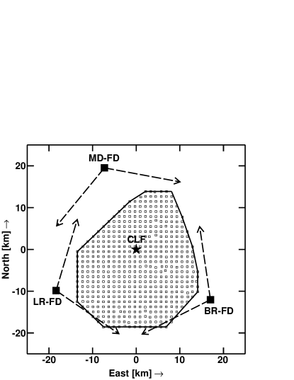
we see the physical layout of all components of TA. Each SD counter consists of two layers of plastic scintillator, 3 m2 in area, and read out independently by two photomultiplier tubes. Scintillation light is guided to the photomultiplier tubes by a system of wavelength-shifting fibers set in grooves in the scintillator. These counters are calibrated every 10 minutes [14] using a histogram of pulse heights recorded for events triggering both layers of scintillators in time coincidence. The resulting distributions typically consist of a peak at low integrated pulse area, accompanied by a tail toward higher pulse area. The peak itself corresponds to the signal from single muons passing through both scintillators, and the centroid of the peak then defines the average signal for a minimum-ionizing particle (MIP) for that channel.
The waveforms from the two scintillators are sampled by a 50 MHz FADC system [14]. A real time integration process is used to trigger each counter: waveforms of pulses with integrated areas corresponding to at least 1/3 MIPs are saved with a corresponding GPS time stamp. The detection of a pulse of 3 MIPs or larger is reported to a central data acquisition system via the radio communication system. A trigger for the TA SD occurs when three adjacent counters have energy deposits equivalent to at least three MIPs in each counter within an 8 sec window. When the SD trigger conditions are met, all counters in the array are polled. Saved waveforms (of minimum 1/3 MIPs) with time stamps within 64 microseconds of the event trigger are read out over the radio link. The pulse area contained in recorded waveforms, stored in raw FADC units, are converted to units of vertical-equivalent muons (VEM). A vertical minimum-ionizing muon deposits on average 2.05 MeV of ionization energy in each scintillator layer. The conversion process uses the calibration histograms collected every 10 minutes, but also incorporates the simulated detector response to single muons and other secondary particles produced in air showers induced by TeV cosmic rays.
The application of the calibration and the signal analysis extract the following information from each counter participating in the event: (a) An integrated particle count in units of VEM, (b) the arrival time of the shower, and (c) the spatial coordinates of the counter. These quantities are then used to reconstruct the shower trajectory and the energy of the primary cosmic ray. Figure 2
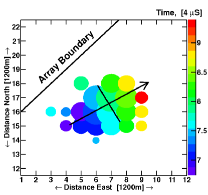
shows a footprint of a typical high energy event.
3 Event Reconstruction and Selection Cuts
The event reconstruction procedures used for TA SD data are based on parametrizations and procedures originally developed by the AGASA Collaboration [15], modified to match the characteristics of the TA detectors [16].
First, the shower axis is determined from the arrival times in the triggered counters. These are fit to the AGASA-modified Linsley time delay function [17][18]. Figure 3a,
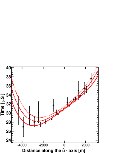
shows this fit for a typical TA SD event. For this work, the parameters of the original AGASA time delay function were adjusted to fit the overall characteristics of the TA SD data set, by considering the distributions of fit residual in distance-to-core, VEM signal sizes, and in zenith angle. It should be emphasized that the adjustments were made based exclusively on actual TA SD data without any additional information from simulations, and are therefore model-independent.
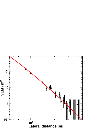
The primary energy estimation of TA SD events is established by first measuring the charge density at 800m in lateral (perpendicular) distance from the shower axis () [5]. The measured particle densities from the counters are fit to the modified AGASA lateral distribution function (LDF) [19], as shown in Figure 3b. The value at 800m, denoted as , is interpolated from this fit.
In order to achieve reasonable detector resolutions in energy and pointing direction, but without losing an unreasonable fraction of events, we chose the following event selection cuts (both pre- and post- reconstruction). These same cuts are applied to both data and Monte-Carlo in the present TA SD analysis:
-
1.
. At least 5 good counters per event.
-
2.
. Zenith angle less than 45 degrees.
-
3.
m. Core position is within the array and at least 1200 m away from the edge of the array.
-
4.
and . Reduced values of of geometry () and LDF () fits are less than 4.
-
5.
. Pointing direction uncertainty is less than 5 degrees. and are the uncertainties on zenith and azimuthal angles from the geometry fit.
-
6.
. Fractional uncertainty of determination (from the LDF fit) is within 25%.
Table 1 displays the efficiency (fraction of events retained) when the quality cuts are applied, incrementally for 3 energy slices.
| Quality cut | Efficiency, | Efficiency, | Efficiency, |
| eV | eV | eV | |
| 0.674 | 0.931 | 0.973 | |
| 0.741 | 0.702 | 0.677 | |
| m | 0.865 | 0.814 | 0.748 |
| 0.928 | 0.938 | 0.981 | |
| 0.656 | 0.925 | 0.995 | |
| 0.534 | 0.887 | 0.995 | |
| All cuts combined | 0.14 | 0.41 | 0.48 |
4 Surface Detector Monte Carlo Simulation
In simulating an air shower, the TA surface detector Monte Carlo uses the CORSIKA 6.960 [7] simulation package. For the standard simulated event set, we selected the QGSJET-II-03 [20] and FLUKA2008.3c [21][22] hadronic models for high and low energies, respectively. For electromagnetic processes, the EGS4 [23] electromagnetic model was used.
The first step in generating a comprehensive simulation of the TA SD data set is to create a library of thinned CORSIKA showers. This library consists of 16,800 extensive air showers with primary energies distributed in bins between eV and eV. The number of showers in each bin ranges from 1000 in the lowest energy bin to 250 in the highest energy bin. These showers are simulated with zenith angles from to assuming an isotropic distribution. It is important to note that in our final analysis we only include events with eV and . However, events must be simulated well beyond these limits in energy and inclination in order to give a complete understanding of our detector acceptance as well as our energy and angular resolutions.
Each shower in the CORSIKA library is then subjected to dethinning [9]. For each simulated event, all shower particles that strike the ground are divided spatially by their landing spots into “tiles” on the desert floor and into wide bins by their arrival time. The total energy deposited by all particles that landed in a particular tile, and into a virtual TA SD counter located at its center, is calculated using the GEANT4 simulation package [24]. Note this analysis assumes many more virtual SD counters (spaced every 6 m instead of 1.2 km) than are actually present in the experiment. Back scattering of particles striking the ground within the tile is included in the simulation. The energy deposited as a function of time is stored in the shower library. Figure 4
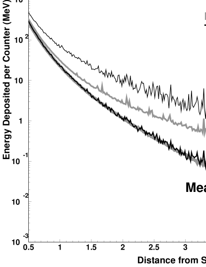
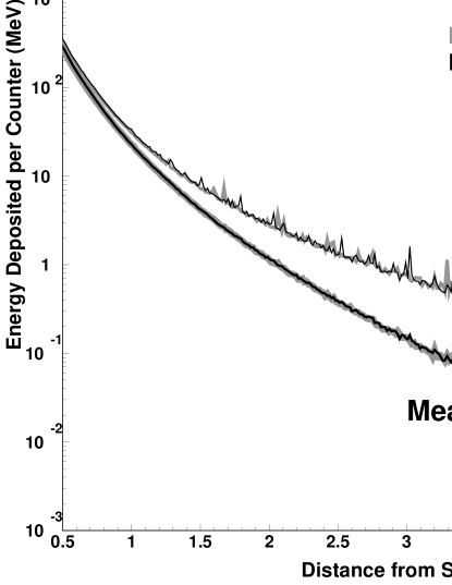
shows the comparison of energy deposition in SD counters vs. distance-to-core from a simulated eV shower before and after de-thinning. The plot on the right, made using a de-thinned shower, shows excellent agreement to an identical unthinned shower in both the mean energy deposit and its RMS variation, plotted as functions of distance-to-core. In contrast, the same plot on the left comparing the same shower after thinning to the same unthinned shower shows a discrepancy in the RMS variation in energy deposition by up to an order of magnitude.
In the concluding step of the shower library generation, each tiled shower is sampled 2000 times through a detailed simulation of the detector, including electronics. The shower core positions, the azimuth of the shower axis, and event times are varied in this process. The detector simulation utilizes real-time calibration information from the TA SD to effect a highly detailed, time-specific simulation of the detector operating conditions. Additionally, random background particles are inserted into the electronics readout based on secondary flux derived from additional CORSIKA simulations of the low-energy cosmic ray spectrum reported by the BESS Collaboration [25]. The net result of this step is to convert each dethinned CORSIKA shower into an event library of simulated detector events in a data format identical to that produced by the TA SD instrumentation.
In order to achieve a highly accurate representation of the actual TA SD data set, we sample simulated events from our event library with a primary energy distribution and composition according to published HiRes energy spectrum [3] and composition [26], respectively. The resulting MC event set is then processed by the same analysis program as the TA SD data. This process chain is illustrated by the diagram in Figure 5.

Finally, we validate the accuracy of the simulation by comparing distributions of key observables obtained from the MC events with those from real data. As will be seen in the next section, our de-thinned shower samples give excellent agreement in these data-MC comparisons, thereby verifying the reliability of detector resolutions and of the detector acceptance calculation obtained from our simulation algorithm. The primary advantage of this process lies in that the trigger efficiency, reconstruction quality cuts, and the effects of finite resolution [27][28] are all automatically included in the analysis.
A functional relationship between , the primary zenith angle (), and the primary energy is constructed using the de-thinned Monte Carlo Event set. Each simulated event is subjected to the same geometrical reconstruction as described above, and the value of obtained in the same way. A three-dimensional scatter plot is then made of the input (generated) primary energy of each shower plotted in the -direction, vs. in the -direction, and the logarithm of the value in the -direction. The points in this plot form a surface that represents the shower energy as a bi-variate function of and . The function obtained for this work is shown in Figure 6,
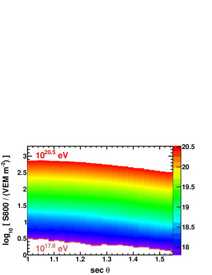
in which the value of energy is represented by color according to the key attached to the right of the plot. The information contained in Figure 6 is used to determine the energy of both real and simulated events from the interpolated values.
5 Data - Monte Carlo Comparisons
A crucial part of the TA SD simulation program is the comparison of data and MC distributions. The success of these comparisons validates the accuracy of the simulated event set in its representation of the real data set, and demonstrates the reliability of analysis procedures that depend on the Monte Carlo. These include the construction of energy vs. and plot in Figure 6, the determination of detector resolutions, and the acceptance calculation.
Figure 7
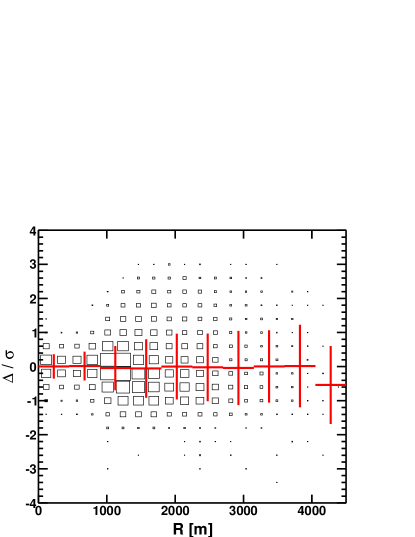
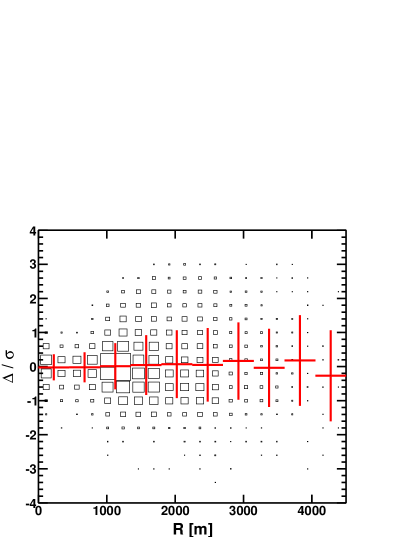
shows normalized residuals of the time fit as a function of lateral distance from the shower core (i.e. the difference between the SD counter time and the fit value, all divided by the uncertainty in counter time). In Figure 7b, we apply the same time delay function to simulated events. In Figure 8, we compare the real and simulated distributions for several geometric observables. By considering the comparison of Figures 7 and 7b in conjunction with the further comparisons shown in Figure 8,
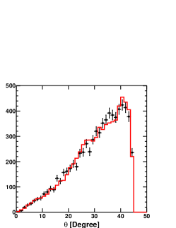
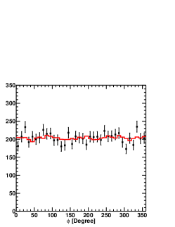
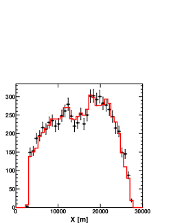
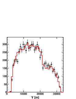
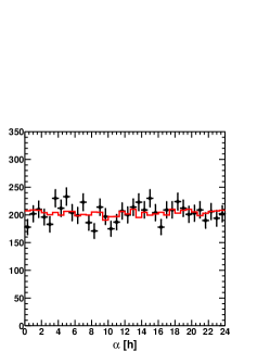
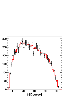
we establish that the simulated event set possesses a distribution of geometric characteristics that are very similar to those of the real data.
Figure 9
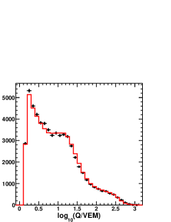
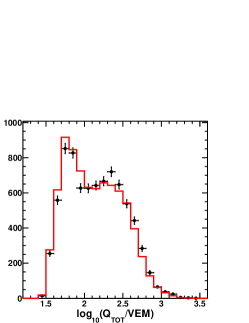
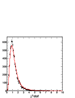
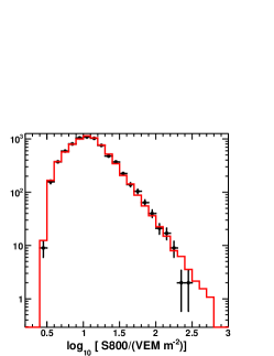
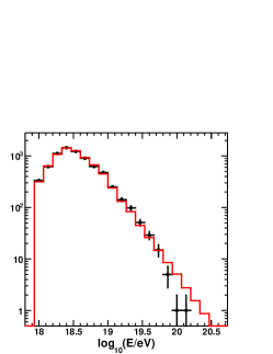
shows the data-MC comparison of real and simulated lateral distribution quantities and the reconstructed energy. It should be noted that while the comparison Figures 9d and 9e show a small deficit of events at large values of and energy in the data, this difference is expected because we do not include the simulation of the GZK suppression [1][2] at this level of analysis, and it does not reflect a fundamental disagreement between the real and simulated event sets. The data-Monte Carlo comparison plots show excellent agreement.
6 Detector Resolutions
The detector resolutions are determined by comparing the reconstructed and generated values for those simulated showers that survived the event selection cuts described in the previous section. The two key resolutions of interest are those of the arrival direction (of particular importance in anisotropy studies) and primary energy (important for the energy spectrum and for anisotropy).
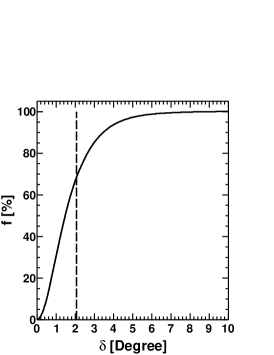
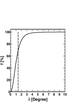
The angular resolution is obtained from a cumulative histogram of the opening angle between the reconstructed event direction and the true (MC generated) direction :
| (1) |
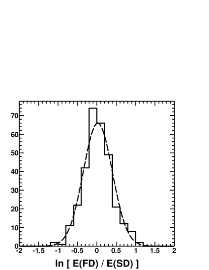
The unit vectors and are calculated from the shower zenith and azimuthal angles (both reconstructed and generated). Figure 10 shows the cumulative distribution of from a spectral MC set (i.e., one generated according to the published HiRes energy spectrum and composition). The results are displayed for three energy ranges. Choosing the 68% confidence interval for stating the answers, the TA SD angular resolution values are: 2.4o for , 2.1o for , and 1.4o for .

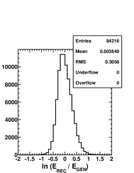
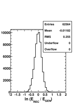
For the energy resolution we state the root-mean-square (RMS) deviation for the distribution of , the ratio of the reconstructed () to the generated () event energies. However, for the display of the distribution of , and for calculating the RMS resolution, it is advantageous to histogram the natural logarithm of the energy ratio, , because treats fractional under-reconstruction and over-reconstruction of event energies in a symmetric way. In contrast, a histogram of just the ratios, , would not properly account for those events with under-reconstructed energies, because is artificially bounded at zero on the low side, but unbounded on the high side. This bias can lead to an understated RMS value and hence overstated resolution.
The RMS deviation of the distribution of the (natural) logarithm of the can also be used to calculate , the fractional energy resolution, according to the first order approximation:
| (2) |
Figure 11 shows the energy resolution of the TA SD for three MC generated energy ranges. The histograms were produced using the MC spectral sets with varying statistics (10 to 40 times that of the real data) to yield similar numbers of events in the histograms. Using the RMS deviation of the distributions and equation 2, the following results were obtained for the TA SD energy resolution (in percents of the true energy): 36% for , 29% for , and 19% for .

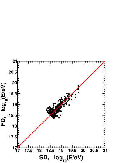
7 Normalizing the Energy Scale
The energy of an air shower seen by a fluorescence detector can be measured accurately because the fluorescence process is basically calorimetric. However for the tails of an air shower, which are observed by a surface detector, one is subject to a much larger uncertainty in energy, which comes from the details of the hadronic generator program used (in our case QGSJET-II). The size of this uncertainty is unknown. Therefore a hybrid experiment, like the Telescope Array, has available to it an excellent way of normalizing its SD energy scale: for events seen by both detectors determine the energy from each detector and normalize the SD energy scale to that of the FD. We observe a 27% difference between the two energy scales, which is independent of energy (SD is higher than FD). We therefore lower the energies of our SD events by this ratio. Figure 12 shows a scatter plot of events’ energies from the FD and SD after this correction is made. This normalization is subject to the systematic uncertainty of the TA FD energy scale, which is 22% [29].
8 Study of Systematic Errors
While calculating the acceptance of the TA surface detector, as is described above, it is possible to estimate the uncertainty in the acceptance values from systematic sources. In this section we describe such estimates for four sources of systematic uncertainty: the attenuation correction used to determine events’ energies as a function of and zenith angle, changing cuts used to remove poorly reconstructed events, unfolding the SD energy resolution, and the small mismatch between data and Monte Carlo distributions of important quantities.
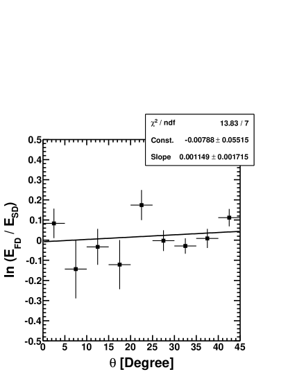
8.1 Attenuation of S800
The attenuation correction arises because at different zenith angles a shower traverses different amounts of atmospheric material before it reaches the ground and is thus observed at a different stage of shower development. We check the systematic uncertainties of attenuation by comparing the dependence of the ratio of FD over SD energies plotted versus the event zenith angle, for events well reconstructed by the FD and SD (the same events used in producing plots in Figure 12). Figure 13 shows the result. To measure a possible bias in our attenuation correction, we fit the ratios to a straight line. The slope of the line is , showing that no bias can be seen with the current statistical power of the data.
8.2 Acceptance
An acceptance bias can occur if there are disagreements between the data and the Monte-Carlo in quantities that are used for making quality cuts. While most quantities agree on a level (the answer is obtained by counting the differences in the numbers of events between the data and MC in each bin and dividing that by the total number of events), there are important exceptions, where the peaks of the data and MC histograms do not match exactly, i.e. data and MC histograms are slightly shifted with respect to each other and simply counting the event differences in bins does not work. One such quantity is the fractional uncertainty in , shown in Figure 14.
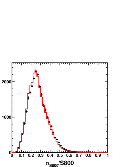
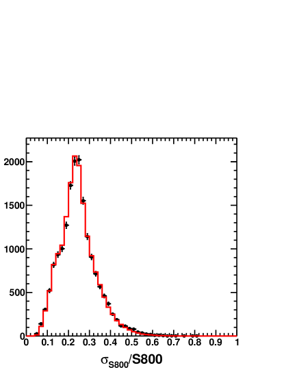
This quantity is used for making the quality cuts: . To determine the systematic uncertainty (effect on the flux) due to this cut, we consider the data and Monte-Carlo ratio:
| (3) |
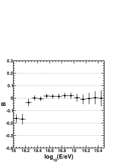
where and are numbers of events reconstructing in the () energy bin for data and Monte-Carlo, respectively. The systematic uncertainty can be readily estimated by calculating with the cut () and without the cut () and evaluating the fractional difference:
| (4) |
Figure 15 shows the bias, , evaluated for the cut on . It shows the systematic change due to the cut is for eV. If one chooses energies eV for calculating the TA SD spectrum, one can avoid any bias as shown in Figure 15.
8.3 Resolution Unfolding
In calculating the energy spectrum, the resolution of the detector (especially if it is non-Gaussian), coupled with a spectrum that rapidly falls with energy, can bias the result. Consequently, we must make a first-order resolution correction in the spectrum calculation. The formula we use is:
| (5) |
where is the flux, is the number of events observed in an energy bin, is the number of accepted simulated events in the energy bin, and is the number of thrown simulated events. The surface area, solid angle acceptance, and live time of the detector are repesented by , and , respectively. Finally, is the reconstructed energy, while is the thrown energy.
In the case of an ideal detector with perfect resolution and 100% efficiency, and . For a real detector with finite resolution and less than perfect efficiency, the ratio performs two important roles. First, compensates for detector efficiency. Second, by binning in but in , we perform a first order (bin-by-bin) correction for energy resolution. The validity of this correction is contigent upon energy resolution that is the same size or smaller than the energy binning used in the calculation, accurate simulation of the energy resolution (as established by the excellent agreement between data and simulation for the of the lateral distribution fits in Figure 9c), and the use of a reasonably accurate input spectral index for the simulation.
If there is a sharp bend in the spectrum, for example the GZK cutoff, the spectrum put into the Monte Carlo should also have the sharp bend, to achieve the best accuracy. While we did not include the effect in the MC for the Data-MC comparison earlier, the GZK cut-of, as previously observed by HiRes, was included in the aperture calculation for the spectrum measurement. The result for the TA SD spectrum is a level of resolution-generated bias that is much smaller than the statistical power of the experiment.
8.4 Uncertainty in Energy Scale and Flux
The systematic uncertainty on the flux due to the systematic uncertainty of the energy scale can be estimated as follows:
| (6) |
where is the measured spectral index. The spectral index for the TA SD spectrum above the ankle is taken from the publication describing the measurement [13]: and the systematic uncertainty of the energy scale is controlled by the TA FD: [29]. Together, these results give . The fluorescence energy scale uncertainty dominates the systematic uncertainty in energy at . All other contributions explored here change the answer by . Thus the total systematic uncertainty in is 37%.
9 Conclusion
We have demonstrated that the dethinned CORSIKA/QGSJET-II-03 proton Monte Carlo simulation accurately models the response of the TA array of scintillation counters to cosmic rays in the eV, domain. In reconstruction of events, fits to counter times and pulse heights are almost identical for the Monte Carlo and the data. Basic histograms of geometrical quantities, and of quantities related to the lateral distribution of counter pulse heights, for the Monte Carlo agree very well with the same distributions for the data. We have measured a 27% correction to the energy scale of the CORSIKA + QGSJET-II simulation package based on air showers observed calorimetrically by the Telescope Array fluorescence detector, and examined some sources of systematic errors in our aperture calculation. We conclude that this Monte Carlo simulation is an accurate tool for calculating the surface detector aperture used to calculate the energy spectrum, as well as to estimate the exposure on the sky for cosmic ray anisotropy analyses.
10 Acknowledgments
The Telescope Array experiment is supported by the Japan Society for the Promotion of Science through Grants-in-Aid for Scientific Research on Specially Promoted Research (21000002) “Extreme Phenomena in the Universe Explored by Highest Energy Cosmic Rays”, and the Inter-University Research Program of the Institute for Cosmic Ray Research; by the U.S. National Science Foundation awards PHY-0307098, PHY-0601915, PHY-0703893, PHY-0758342, and PHY-0848320 (Utah) and PHY-0649681 (Rutgers); by the National Research Foundation of Korea (2006-0050031, 2007-0056005, 2007-0093860, 2010-0011378, 2010-0028071, R32-10130); by the Russian Academy of Sciences, RFBR grants 10-02-01406a and 11-02-01528a (INR), IISN project No. 4.4509.10 and Belgian Science Policy under IUAP VI/11 (ULB). The foundations of Dr. Ezekiel R. and Edna Wattis Dumke, Willard L. Eccles and the George S. and Dolores Dore Eccles all helped with generous donations. The State of Utah supported the project through its Economic Development Board, and the University of Utah through the Office of the Vice President for Research. The experimental site became available through the cooperation of the Utah School and Institutional Trust Lands Administration (SITLA), U.S. Bureau of Land Management and the U.S. Air Force. We also wish to thank the people and the officials of Millard County, Utah, for their steadfast and warm support. We gratefully acknowledge the contributions from the technical staffs of our home institutions and the University of Utah Center for High Performance Computing (CHPC).
References
- [1] K. Greisen, End of the cosmic-ray spectrum?, Phys. Rev. Lett. 16 (1966) 748.
- [2] G. T. Zatsepin, V. A. Kuzmin, Upper limit of the spectrum of cosmic rays, JETP Lett. 4 (1966) 78–80.
- [3] R. U. Abbasi, et al., Observation of the GZK cutoff by the HiRes experiment, Phys. Rev. Lett. 100 (2008) 101101. arXiv:astro-ph/0703099, doi:10.1103/PhysRevLett.100.101101.
- [4] J. Abraham, et al., Observation of the suppression of the flux of cosmic rays above eV, Phys. Rev. Lett. 101 (2008) 061101. arXiv:0806.4302, doi:10.1103/PhysRevLett.101.061101.
- [5] D. Newton, J. Knapp, A. A. Watson, The optimum distance at which to determine the size of a giant air shower, Astropart. Phys. 26 (2007) 414–419. arXiv:astro-ph/0608118, doi:10.1016/j.astropartphys.2006.08.003.
- [6] A. Hillas, Shower simulation: Lessons from MOCCA, Nucl.Phys.Proc.Suppl. 52B (1997) 29–42. doi:10.1016/S0920-5632(96)00847-X.
- [7] D. Heck, G. Schatz, T. Thouw, J. Knapp, J. N. Capdevielle, CORSIKA: A Monte Carlo code to simulate extensive air showers, Tech. Rep. 6019, FZKA (1998).
- [8] S. J. Sciutto, AIRES: A system for air shower simulations, Tech. Rep. 2.6.0, UNLP (2002).
- [9] B. T. Stokes, et al., Dethinning extensive air shower simulations, Astropart. Phys. 35 (2012) 759. arXiv:1104.3182.
- [10] B. T. Stokes, et al., A simple parallelization scheme for extensive air shower simulations, submitted to Nuclear Instruments and Methods (2011). arXiv:1103.4643.
- [11] H. Kawai, et al., Telescope Array Experiment, Nucl. Phys. Proc. Suppl. 175-176 (2008) 221–226. doi:10.1016/j.nuclphysbps.2007.11.002.
- [12] H. Tokuno, et al., The Telescope Array Experiment: Status and prospects, J. Phys. Conf. Ser. 120 (2008) 062027. doi:10.1088/1742-6596/120/6/062027.
- [13] T. Abu-Zayyad, et al., The cosmic ray energy spectrum observed with the surface detector of the Telescope Array experiment, Astrophys.J. 768 (2013) L1. arXiv:1205.5067, doi:10.1088/2041-8205/768/1/L1.
- [14] T. Nonaka, et al., Performance of TA surface array, in: Proceedings of the 31st ICRC, Łódź, 2009.
- [15] M. Takeda, N. Sakaki, K. Honda, M. Chikawa, M. Fukushima, et al., Energy determination in the Akeno Giant Air Shower Array experiment, Astropart.Phys. 19 (2003) 447–462. arXiv:astro-ph/0209422, doi:10.1016/S0927-6505(02)00243-8.
- [16] G. B. Thomson, Results from the Telescope Array Experiment, in: Proceedings of Science (ICHEP 2010), 2010, p. 448. arXiv:1010.5528.
- [17] J. Linsley, The structure function of EAS measured at Volcano Ranch, Conf. Proc. C750815V8 (1975) 2746.
- [18] M. Teshima, et al., Properties of 109 GeV–1010GeV extensive air showers at core distances between 100 m and 3000 m, J. Phys. G12 (1986) 1097. doi:10.1088/0305-4616/12/10/017.
- [19] K. Shinozaki, M. Teshima, AGASA results, Nucl. Phys. Proc. Suppl. 136 (2004) 18–27. doi:10.1016/j.nuclphysbps.2004.10.045.
- [20] S. Ostapchenko, QGSJET-II: Towards reliable description of very high energy hadronic interactions, Nucl. Phys. Proc. Suppl. 151 (2006) 143–146. arXiv:hep-ph/0412332, doi:10.1016/j.nuclphysbps.2005.07.026.
- [21] A. Ferrari, P. R. Sala, A. Fasso, J. Ranft, FLUKA: A multi-particle transport code (Program version 2005), Tech. Rep. 2005-010, CERN (2005).
- [22] G. Battistoni, et al., The FLUKA code: Description and benchmarking, AIP Conf. Proc. 896 (2007) 31–49. doi:10.1063/1.2720455.
- [23] W. R. Nelson, H. Hirayama, D. W. O. Rogers, The EGS4 code system, Tech. Rep. 0265, SLAC (1985).
- [24] J. Allison, et al., GEANT4 developments and applications, IEEE Trans. Nucl. Sci. 53 (2006) 270. doi:10.1109/TNS.2006.869826.
- [25] T. Sanuki, et al., Precise measurement of cosmic-ray proton and helium spectra with the BESS spectrometer, Astrophys. J. 545 (2000) 1135. arXiv:astro-ph/0002481, doi:10.1086/317873.
- [26] R. U. Abbasi, et al., Indications of proton-dominated cosmic ray composition above 1.6 EeV, Phys. Rev. Lett. 104 (2010) 161101. arXiv:0910.4184, doi:10.1103/PhysRevLett.104.161101.
- [27] G. Cowan, A survey of unfolding methods for particle physics, in: Prepared for Conference on Advanced Statistical Techniques in Particle Physics, Durham, England, 2002.
- [28] R. U. . Abbasi, et al., Monocular measurement of the spectrum of UHE cosmic rays by the FADC detector of the HiRes experiment, Astropart. Phys. 23 (2005) 157–174. arXiv:astro-ph/0208301, doi:10.1016/j.astropartphys.2004.12.006.
- [29] T. Abu-Zayyad, et al., TA Energy Scale: Methods and Photometry, in: Proceedings of the 32nd ICRC, Vol. 2, Beijing, 2011, p. 250.