Bayesian Density Estimation via Multiple Sequential Inversions of 2-D Images with Application in Electron Microscopy

Authors’ affiliations:

¹Associate Research Fellow in Department of Statistics, University of Warwick, Coventry CV4 7AL, U.K., corresponding author,
⁶Lecturer of Statistics, Department of Mathematics, University of Leicester, Leicester LE1 7RH, U.K.,
²Research Biostatistics Group Head, Novartis Vaccines and Diagnostics and Associate fellow at Department of Statistics, University of Warwick,
³Graduate student at Emerging Technologies Research Centre, De Montfort University,
⁴Lecturer, Department of Physics, University of Warwick,
⁵Head, Emerging Technologies Research Centre, De Montfort University

Abstract

We present a new Bayesian methodology to learn the unknown material density of a given sample by inverting its two-dimensional images that are taken with a Scanning Electron Microscope. An image results from a sequence of projections of the convolution of the density function with the unknown microscopy correction function that we also learn from the data. We invoke a novel design of experiment, involving imaging at multiple values of the parameter that controls the sub-surface depth from which information about the density structure is carried, to result in the image. Real-life material density functions are characterised by high density contrasts and typically are highly discontinuous, implying that they exhibit correlation structures that do not vary smoothly. In the absence of training data, modelling such correlation structures of real material density functions is not possible. So we discretise the material sample and treat values of the density function at chosen locations inside it as independent and distribution-free parameters. Resolution of the available image dictates the discretisation length of the model; three models pertaining to distinct resolution classes are developed. We develop priors on the material density, such that these priors adapt to the sparsity inherent in the density function. The likelihood is defined in terms of the distance between the convolution of the unknown functions and the image data. The posterior probability density of the unknowns given the data is expressed using the developed priors on the density and priors on the microscopy correction function as elicitated from the Microscopy literature. We achieve posterior samples using an adaptive Metropolis-within-Gibbs inference scheme. The method is applied to learn the material density of a 3-D sample of a nano-structure, using real image data. Illustrations on simulated image data of alloy samples are also included.

Keywords: Bayesian methods, Inverse Problems, Nonparametric methods, Priors on sparsity, Underdetermined problems

1 Introduction

Nondestructive learning of the full three-dimensional material density function in the bulk of an object, using available two dimensional images of the object, is an example of a standard inverse problem (?; ?; ?; ?; ?). The image results from the projection of the three dimensional material density onto the image plane. However, inverting the image data does not lead to a unique density function in general; in fact to render the inversion unique, further measurements need to be invoked. For instance, the angle at which the object is imaged or viewed is varied to provide a series of images, thereby expanding available information. This allows to achieve ditinguishability (or identifiability) amongst the solutions for the material density. A real-life example of such a situation is presented by the pursuit of material density function using noisy 2-dimensional (2-D) images taken with electron microscopy techniques (?). Such non-invasive and non-destructive 3-D density modelling of material samples is often pursued to learn the structure of the material in its depth (?), with the ulterior aim of controlling the experimental conditions under which material samples of desired qualities are grown.

Formally, the projection of a density function onto a lower dimensional image space is referred to as the Radon Transform; see ?, ?. The inverse of this projection is also defined but requires the viewing angle as an input and secondly, involves taking the spatial derivative of the density function, rendering the computation of the inverse projection numerically unstable if the image data is not continuous or if the data comprises limited-angle images (?; ?) or if noise contaminates the data (?). Furthermore, in absence of measurements of the viewing angle, the implementation of this inverse is not directly possible, as ? suggested. Even when the viewing angle is in principle measurable, logistical difficulties in imaging at multiple angles result in limited-angle images. For example, in laboratory settings, such as when imaging with Scanning Electron Microscopes (SEMs), the viewing angle is varied by re-mounting the sample on stubs that are differently inclined each time. This mounting and remounting of the sample is labour-intensive and such action leads to the breaking of the vacuum within which imaging needs to be undertaken, causing long waiting periods between two consecutive images. When vacuum is restored and the next image is ready to be taken, it is very difficult to identify the exact fractional area of the sample surface that was imaged the last time, in order to scan the beam over that very area. In fact, the microscopist would prefer to opt for an imaging technique that allows for imaging without needing to break the vacuum in the chamber at all. Such logistical details are restrictive in that this allows imaging at only a small number of viewing angles, which can cause the 3-D material density reconstruction to be numerically unstable. This problem is all the more acute when the data is discontinuous and heterogeneous in nature. Indeed, with the help of ingenious imaging techniques such as compressive sensing (?), the requirement of a large number of image data points is potentially mitigated. If implemented, compressive imaging would imply averaging the image data over a chosen few pixels, with respect to a known non-adaptive kernel. Then the inversion of such compressed data would require the computation of one more averaging or projection (and therefore one more integration) than are otherwise relevant. While this is easily done, the implementation of compressive sensing of electron microscopy data can be made possible only after detailed instrumentational additions to the imaging paraphernalia is made. Such instrumentational additions are outside the scope of our work. We thus invoke a novel design of imaging experiment that involves imaging at multiple values of some relevant parameter that is easily varied in a continuous way over a chosen range, unlike the viewing angle. In this paper, we present such an imaging strategy that allows for multiple images to be recorded, at each value of this parameter, when a cuboidal slab of a material sampe is being imaged with an SEM.

In imaging with an SEM, the projection of the density function is averaged over a 3-D region inside the material, the volume of which we consider known; such a volume is indicated in the schematic diagram of this imaging technique shown in Figure 1. Within this region, a pre-fixed fraction of the atomistic interactions between the material and the incident electron beam stay confined, (?; ?). The 2-D SEM images are taken in one of the different types of radiation that are generated as a result of the atomistic interactions between the molecules in the material and a beam of electrons that is made incident on the sample, as part of the experimental setup that characterises imaging with SEM, (?; ?; ?). Images taken with bulk electron microscopy techniques potentially carry information about the structure of the material sample under its surface, as distinguished from images obtained by radiation that is reflected off the surface of the sample, or is coming from near the surface.

In practice, the situation is rendered more complicated by the fact that for the 2-D images to be formed, it is not just the material density function, but the convolution of the material density function with a kernel that is projected onto the image space. The nature of the modulation introduced by this kernel is then also of interest, in order to disentangle its effect from that of the unknown density function that is responsible for generating the measured image. As for the modulation, both enhancement and depletion of the generated radiation is considered to occur in general. It is to be noted that this kernel is not the measure of blurring of a point object in the imaging technique, i.e. it is not the point spread function (PSF) of the observed image, but is characteristic of the material at hand. The kernel really represents the unknown microscopy correction function that convolves with the material density function–this convolution being projected to form the image data, which gets blurred owing to specifics of the imaging apparataus. Learning the de-blurred image from the PSF-convolved image data is an independent pursuit, referred to as Blind Deconvolution (?; ?; ?). Here our aim is to learn the material density and the microscopy correction function using such noisy image data.

The convolution of the unknown kernel with the unknown density, is projected first onto the 2-D surface of the system, and the resulting projection is then successively marginalised over the 2 spatial coordinates that span the plane of the system surface. Thus, three successive projections result in the image data. Here we deal with the case of an image resulting from a composition of a sequence of three independent projections of the convolution of the material density function and the unknown kernel or microscopy function. So only a sequence of inversions of the image allow us to learn this density. Such multiple inversions are seldom addressed in the literature, and here, we develop a Bayesian method that allows for such successive inversions of the observed noisy, PSF-convolved 2-D images, in order to learn the kernel as well as the density function. The simultaneous pursuit of both the unknown density and the kernel, is less often addressed than are reported attempts at density reconstruction, under an assumed model for the kernel, (?; ?; ?; ?).

We focus here on the learning of a density function that is not necessarily convex, is either sparse or dense, is often multimodal - with the modes characterised by individualised, discontinuous substructure and abrupt bounds, resulting in the material density function being marked by isolated islands of overdensity and sharp density contrasts; we shall see this below in examples of reconstructed density functions presented in Section 9 and Section 10. Neither the isolated modes of the material density function in real-life material samples nor the adjacent bands of material over-density, can be satisfactorily modelled with a mixture model. Again, modelling of such a real-life trivariate density function with a high-dimensional Gaussian Process (GP) is not possible in lieu of training data, given that the covariance function of the invoked GP will then have to be non-stationary (?) and exhibit non-smooth spatial variation. Here by “training data” is implied data comprising a set of known values of the material density, at chosen points inside the sample; such known values of the density function are unknown. Even if the covariance function were varying smoothly over the 3-D spatial domain its parametrisation is $adhoc$ in lieu of training data but with an abruptly evolving covariance function–as in the problem of inverting SEM image data–such parametrisation becomes impossible (?), especially when there is no training data available. At the same time, the blind implementation of the inverse Radon Transform would render the solution unstable given that the distribution of the image data in real-life systems is typically, highly discontinuous.

In the following section, (Section 2) we describe the experimental setup delineating the problem of inversion of the 2-D images taken with Electron Microscopy imaging techniques, with the aim of learning the sub-surface material density and the kernel. In addition, we present the novel design of imaging experiment that achieves multiple images. In Section 3 we discuss the outstanding difficulties of multiple and successive inversions and qualitatively explain the relevance of the advanced solution to this problem. This includes a discussion of the integral representation of the multiple projections (Section 3.2), the outline of the Bayesian inferential scheme adopted here (Section 3.6) and a section on the treatment of the low-rank component of the unknown material density (section 3.5). The details of the microscopy image data that affect the modelling at hand are presented in the subsequent section. This includes a description of the 3 models developed to deal with the three classes of image resolution typically encountered in electron microscopy (Section 3.3) and measurement uncertainties of the collected image data (Section 3.4). Two models on the kernel, as motivated by small and high levels of information available on the kernel given the material at hand are discussed in Section 4; priors on the parameters of the respective models is discussed here as well. Section 5 is devoted to the development of priors on the unknown density function such that the priors are adaptive to the sparsity in the density. In Section 6, the discretised form of the successive projections of the convolution of the unknown functions is given for the three different models. Inference is discussed in Section 7. Section 8 discusses with salient aspects of the uniqueness of the solutions. Application of the method to the analysis of real Scanning Electron Microscope image data is included in Section 10 while results from the inversion of simulated image data are presented in Section 9. Relevant aspects of the methodology and possible other real-life applications in the physical sciences are discussed in Section 11.

2 Application to Electron Microscopy Image Data

For our application, the system i.e. the slab of material, is modelled as a rectangular cuboid such that the surface at which the electron beam is incident is the $Z$=0 plane. Thus, the surface of the system is spanned by the orthogonal $X$ and $Y$-axes, each of which is also orthogonal to the $Z$-axis that spans the depth of the slab. In our problem, the unknown functions are the material density $\rho(x,y,z)$ and the kernel $\eta(x,y,z)$.

Here we learn the unknown functions by inverting the image data obtained with a Scanning Electron Microscope. Though the learning of the convolution $\rho\ast\eta$ of $\rho(x,y,z)$ and $\eta(x,y,z)$, is in principle ill-posed, we suggest a novel design of imaging experiment that allows for an expansion of the available information leading to $\rho\ast\eta$ being learnt uniquely when noise in the data is small (Section 8). This is achieved by imaging each part of the material sample at $N_{{\textrm{eng}}}$ different values of a parameter $E$ such that images taken at different values $\epsilon$ of this parameter $E$, carry information about the density function from different depths under the sample surface. Such is possible if $E$ represents the energy of the electrons in the incident electron beam that is used to take the SEM image of the system; since the sub-surface penetration depth of the electron beam increases with electron energy, images taken with beams of different energies inherently bear information about the structure of the material at different depths.

The imaging instrument does not image the whole sample all at the same time. Rather, the imaging technique that is relevant to this problem is characterised by imaging different parts of the sample, successively in time. At each of these discrete time points, the $i$-th part, ($i=1,\ldots,N_{{\textrm{data}}}$) of the sample is viewed by the imaging instrument, along the viewing vector ${\boldsymbol{v}}_{i}$ to record the image datum in the $i$-th pixel on the imaging screen. Thus, every pixel of image data represents information about a part of the sample. The $i$-th viewing vector corresponds to the $i$-th point of incidence of the electron beam on the surface of the material sample. The image datum recorded in the $i$-th pixel then results from this viewing, and harbours information about the sample structure inside the $i$-th interaction-volume, which is the region that bounds atomistic interactions between the incident electron beam and molecules of the material (see Figure 1). The point of incidence of the $i$-th viewing vector, i.e. the centre of the $i$-th interaction volume is marked in the diagram. The volume of any such 3-D interaction-volume is known from microscopy theory (?) and is a function of the energy $E$ of the beam electrons. In fact, motivated by the microscopy literature, (?), we model the shape of the $i$-th interaction-volume as hemispherical, centred at the incidence point of $\boldsymbol{v}_{i}$, with the radius of this hemisphere modelled as $\propto E^{1.67}$. We image each part of the sample at $N_{{\textrm{eng}}}$ different values of $E$, such that the $k$-th value of $E$ is $\epsilon_{k}$, $k=1,\ldots,N_{{\textrm{eng}}}$. To summarise, the data comprise a $N_{{\textrm{eng}}}$ 2-D images, each image being a square spatial array of ${N_{{\textrm{data}}}}$ number of pixels such that at the $i$-th pixel, for the $k$-th value of $E$, the image data is $\tilde{I}_{i}^{(k)}$ where $i=1,\ldots,N_{{\textrm{data}}}$. Consideration of this full set of images will then suggest the sub-surface density function of the sample, in a fully discretised model. Convolution $\rho\ast\eta$ of $\rho(x,y,z)$ and $\eta(x,y,z)$ is projected onto the system surface, i.e. the $Z$=0 plane and this projection is then further projected onto one of the $X$ or $Y$ axes, with the resulting projection being projected once again, to the central point of the interaction-volume created by the $i$-th incidence of the beam of energy $\epsilon_{k}$, to give rise to the image datum in the $i$-th pixel in the $k$-th image.

Expanding information by imaging at multiple values of $E$ is preferred to imaging at multiple viewing angles for logistical reason as discussed above in Section 1. Further, the shape of the interaction-volume is rendered asymmetric about the line of incidence of the beam when the beam is tilted to the vertical (?, Figure 3.20 on page 92 of), where the asymmetry is dependent on the tilt angle and the material. Then it is no longer possible to have confidence in any parametric model of the geometry of the interaction-volume as given in microscopy theory. Knowledge of the symmetry of the interaction-volume is of crucial importance to any attempt in inverting SEM image data with the aim of learning the material density function. So in this application, varying the tilt angle will have to be accompanied by approximations in the modelling of the projection of $\rho\ast\eta$. We wish to avoid this and therefore resort to imaging at varying values of $E$.

Physically speaking, the unknown density $\rho(x,y,z)$ would be the material density representing amount or mass of material per unit 3-D volume. The measured image datum could be the radiation in Back Scattered Electrons or X-rays, in each 2-D pixel, as measured by a Scanning Electron Microscope.

$\begin{array}[]{c c}\includegraphics[height=119.9664pt]{epma_pap2.pdf}\includegraphics[height=131.96579pt]{ik.pdf}\end{array}$

Figure 1: Left: schematic diagram of the imaging experiment relevant to the application of inverting image data taken with a Scanning Electron Microscope, to learn sub-surface material density and the kernel. The interaction-volume created by the incidence of the electron beam (shown in thick arrow) is modelled as a hemisphere (shown in blue) centred at the point of incidence of this beam with radius given as a function of the energy $E$ of the beam. At each of the $N_{{\textrm{data}}}$ incidences of the beam, $N_{{\textrm{eng}}}$ images are taken with beams that are distinguished by the energy $E$ of the electrons in them. The $X$, $Y$ and $Z$-axes characterising the 3-dimensional grid used in the modelling are marked. The $i$-th incidence of the beam is on the point $(x_{i},y_{i},0)$ on the sample surface. Right: The $j$-th and $i$-th beam incidences are depicted. At the $i$-th incidence, the interaction-volumes resulting from interactions of the material with beams of energy $E=\epsilon_{k}$ (larger interaction-volume in outline only) and $E=\epsilon_{k-1}$ (smaller interaction-volume in blue) are schematically depicted.

3 Modelling

The general inverse problem is $I={\cal P}(\rho)+\varepsilon$ where the data $I:{\mathbb{R}}^{m}\longrightarrow{\cal D}\subseteq{\mathbb{R}}$, while the unknown function $\rho:{\mathbb{R}}^{n}\longrightarrow{\cal H}\subseteq{\mathbb{R}}$, with $m\leq n$. In particular, 3-D modelling involves the case of $n=3$, $m=2$. The case of $n>m$ is fundamentally an ill-posed problem (?; ?). Here $\varepsilon$ is the measurement noise, the distribution of which, we assume known.

In our application, the data is represented as the projection of the convolution of the unknown functions as:

$${\tilde{I}}={\cal C}[\rho\ast\eta]+\varepsilon,$$

where the projection operator ${\cal C}$ is a contractive projection from the space that $\rho\ast\eta$ lives in - which is $\subseteq{\mathbb{R}}^{3}$ - onto the image space ${\cal D}$. ${\cal C}$ itself is a composition of 3 independent projections in general,

$${\cal C}=P_{1}\circ P_{2}\circ P_{3},$$

where $P_{1}$ is the projection onto the $Z$=0 plane, followed by $P_{2}$ - the projection onto the $Y$=0 axis, followed by $P_{3}$ - projection onto the centre of a known material-dependent three dimensional region inside the system, namely the interaction volume. These 3 projections are commutable, resulting in an effective contractive projection of $\rho\ast\eta$ onto the centre of this interaction volume. Thus, the learning of $\rho\ast\eta$ requires multiple (three) inversions of the image data. In this sense, this is a harder than usual inversion problem. The interaction volume and its centre - at which point the electron beam is incident - are shown in Figure 1.

It is possible to reduce the learning of $\rho\ast\eta$ to a least-squares problem in the low-noise limit, rendering the inverse learning of $\rho\ast\eta$ unique by invoking the Moore Penrose inverse of the matrix ${\bf C}$ that is the matrix representation of the ${\cal C}$ operator (Section 8). The learning of $\rho({x,y,z})$ and $\eta({x,y,z})$ individually, from the uniquely learnt $\rho\ast\eta$ is still an ill-posed problem. In a non-Bayesian framework, a comparison of the number of unknowns with the number of measured parameters is relevant; imaging at $N_{{\textrm{eng}}}$ number of values of $E$ suggests that $N_{{\textrm{data}}}\times N_{{\textrm{eng}}}$ parameters are known while at most $N_{{\textrm{data}}}\times N_{{\textrm{eng}}}+N_{{\textrm{eng}}}$ are unknown. Thus, for the typical values of $N_{{\textrm{eng}}}$ and $N_{{\textrm{data}}}$ used in applications, ratio of known to unknown parameters is $\geq 0.99$, using the aforementioned design of experiment (see Section 8.1). The unknown $N_{{\textrm{eng}}}$ parameters still renders the individual learning of $\rho({x,y,z})$ and $\eta({x,y,z})$ non-unique. Such considerations are however relevant only in the absence of Bayesian spatial regularisation (?; ?), and as we will soon see, the lack of smooth variation in the spatial correlation structure underlying typically discontinuous real-life material density functions, render the undertaking of such regularisation risky.

However in the Bayesian framework we seek the posterior probability of the unknowns given the image data. Thus, in this approach there is no need to directly invert the sequential projection operator ${\cal C}$; the variance of the posterior probability density of the unknowns given the data is crucially controlled by the strength of the priors on the unknowns (?; ?). We develop the priors on the unknowns using as much of information as is possible. Priors on the kernel can be weak or strong depending on information available in the literature relevant to the imaged system. Thus, in lieu of strong priors that can be elicited from the literature, a distribution-free model for $\eta({x,y,z})$ is motivated, characterised by weak priors on the shape of this unknown function. On the contrary, if the shape is better known in the literature for the material at hand, the case is illustrated by considering a parametric model for $\eta({x,y,z})$, in which priors are imposed on the parameters governing this chosen shape. Also, the material density function can be sparse or dense. To help with this, we need to develop a prior structure on $\rho({x,y,z})$ that adapts to the sparsity of the density in its native space. It is in this context, that such a problem of multiple inversions is well addressed in the Bayesian framework.

3.1 Defining a general voxel

Lastly, we realise that the data at hand is intrinsically discrete, owing to the imaging mechanism. Then,

• for a given beam energy, collected image data is characterised by a resolution that depends on the size of the electron beam that is used to take the image, as well as the details of the particular instrument that is employed for the measurements. The SEM cannot “see” variation in structure at lengths smaller than the beam size. In practice, resolution $\omega$ is typically less than the beam size; $\omega$ is given by the microscopist. Then only one image datum is available over an interval of width $\omega$ along each of the $X$ and $Y$-axes, i.e. only one datum is available from a square of edge $\omega$, located at the beam pointing. This implies that using such data, no variation in the material density can be estimated within any square (lying on the $X-Y$ plane) of side $\omega$, located at a beam pointing, i.e. $\rho(x,y,z)=\rho(x+\delta_{1},y+\delta_{2},z)$, where $\delta_{1},\delta_{2}\in[0,\omega)$, $\forall\>x,y,z$. The reason for not being able to predict the density over lengths smaller than $\omega$, in typical real-life material samples, is discussed below.

• image data are recorded at discrete (chosen) values of the beam energy $E$ such that for a given beam pointing, a beam at a given value $\epsilon_{k}$ of $E$ carries information about the material density from within the sub-surface depth of $h^{(k)}$. Then 2 beams at successive values $\epsilon_{k-1}$ and $\epsilon_{k}$ of $E$ allow for estimation of the material density within the depth interval $[h^{(k-1)},h^{(k)})$ that is bounded by the beam penetration depths. Here $k=1,2,\ldots,N_{{\textrm{eng}}}$, $h^{(0)}$=0. This implies that for a given beam pointing, over any such interval, no variation in the material density can be learnt from the data, i.e. $\rho(x,y,z)=\rho(x,y,z+\delta_{3})$ where $\delta_{3}\in[h^{(k-1)},h^{(k)})$, $\forall\>x,y,z$. Again, the reason for inability to predict the density at any $z$ is explained below.

As is evident in these 2 bulletted points above, we are attempting to learn the density at discrete points identified by the resolution in the data. The inability to predict the density at any point inside the sample could be possible in alternative models, for example when a Gaussian Process (GP) prior is used to model the trivariate density function that is typically marked by disjoint support in ${\mathbb{R}}^{3}$ and/or by sharp density contrasts (seen in a real density as in Figure 10 and those learnt from simulated image data, as in Figure 5). While the covariance structure of such a GP would be non-stationary (as motivated in the introductory section), the highly discontinuous nature of real-life density functions would compel this non-stationary covariance function to not vary smoothly. Albeit difficult, the parametrisation of such covariance kernels can in principle be modelled using a training data–except for the unavailability of such training data (comprising known values of density at chosen points inside the given 3-D sample). As training data is not at hand, parametrisation of the non-stationary covariance structure is not possible, leading us to resort to a fully discretised model in which we learn the density function at points inside the sample, as determined by the data resolution. In fact, the learnt density function could then be used as training data in a GP-based modelling scheme to help learn the covariance structure. Such an attempt is retained for future consideration.

Thus, prediction would involve (Bayesian) spatial regularisation which demands modelling of the abruptly varying spatial correlation structure that underlies the highly discontinuous, trivariate density function of real life material samples (see Figure 10). The spatial variation in the correlation structure of the image data cannot be used as a proxy for that of the material density function, since the former is not a pointer to the latter, given that compression of the density information within a 3-D interaction-volume generates an image datum. Only with training data comprising known material density at chosen points, can we model the correlation structure of the density function. In lieu of training data, as in the current case, modelling of such correlation is likely to fail.

Hence we learn the density function at the grid points of a 3-D Cartesian grid set up in the space of $X$, $Y$ and $Z$. No variation in the material density inside the $ik$-th grid-cell can be learnt, where this grid-cell is defined as the “$ik$-th voxel” which is the cuboid given by

1. square cross-sectional area (on a $Z=$constant plane) of size $\omega^{2}$, with edges parallel to the $X$ and $Y$ axes, located at the $i$-th beam incidence,

2. depth along the $Z$-axis ranging from $h^{(k-1)}\leq z<h^{(k)}$,

with $i=1,2,\ldots,N_{{\textrm{data}}}$, $k=1,2,\ldots,N_{{\textrm{eng}}}$, $h^{(0)}=0$. Then one pair of opposite vertices of the $ik$-th voxel are respectively at points $(x_{i},y_{i},h^{(k-1)})$ and $(x_{i},y_{i},h^{(k)})$, where the $i$-th beam incidence is at the point $(x_{i},y_{i},0)$ and

$${x_{i}:=i\>{\textrm{modulo}}\>(\sqrt{N_{{\textrm{data}}}})\quad y_{i}:={\textrm{int}}(i/\sqrt{N_{{\textrm{data}}}})+1.}.$$ (3.1)

See Figure 2 for a schematic depiction of a general voxel. Here $\sqrt{N_{{\textrm{data}}}}$ is the number of intervals of width $\omega$ along the $X$-axis, as well as along the $Y$-axis. Thus, on the part of the $X-Y$ plane that is imaged, there are $N_{{\textrm{data}}}$ squares of size $\omega$. Formally, the density function that we can learn using such discrete image data is represented as

$$\xi^{(k)}_{i}:=\rho(x,y,z)\quad\mbox{for}\quad x\in[x_{i},x_{i}+\omega),y\in[y_{i},y_{i}+\omega),z\in[h^{(k-1)},h^{(k)}),$$ (3.2)

This representation suggests that a discretised version of the sought density function is what we can learn using the available image data. We do not invoke any distribution for the unknown parameters
$\xi^{(1)}_{1},\xi^{(2)}_{1},\ldots,\xi^{(N_{{\textrm{eng}}})}_{1},\xi^{(1)}_{2},\ldots,\xi^{(N_{{\textrm{eng}}})}_{2},\ldots,\xi^{(1)}_{N_{{\textrm{data}}}},\ldots,\xi^{(N_{{\textrm{eng}}})}_{N_{{\textrm{data}}}}$. It is to be noted that the number of parameters that we seek is deterministically driven by the image data that we work with–the discretisation of the data drives the discretisation of the space of $X$, $Y$ and $Z$ and the density in each of the resulting voxels is sought. Thus, when the image has a resolution $\omega$ and there are $N_{{\textrm{eng}}}$ such image data sets recorded at a value of $E$, the number of sought density parameters is $N_{{\textrm{data}}}\times N_{{\textrm{eng}}}$ where $N_{{\textrm{data}}}$ is the number of squares of size $\omega$ that comprise part of the surface of the material slab that is imaged. Here the number of parameters $N_{{\textrm{data}}}\times N_{{\textrm{eng}}}$ is typically large; in the application to real data that we present later, this number is 2250. We set up a generic model that allows for the learning of such large, data-driven number of distribution-free density parameters in a Bayesian framework.

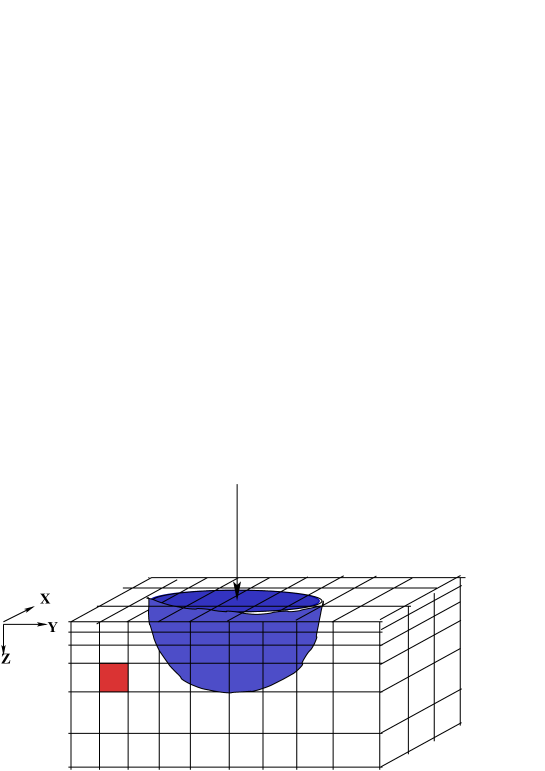
Figure 2: Figure to bring out the general ($ik$-th) voxel, as distinguished from the general ($ik$-th) interaction-volume. For the value $\epsilon_{k}$ of the imaging parameter $E$, the $i$-th viewing vector $\boldsymbol{v}_{i}$ impinges the $Z$=0 surface at the material slab at point $(x_{i},y_{i},0)$, creating the $ik$-th interaction-volume (in blue) that is modelled as a hemisphere of radius $R0^{(k)}$. The maximal depth that this interaction-volume extends to, is $h^{(k)}$. Thus, under the assumption of hemi-spherical shape, $R0^{(k)}=h^{(k)}$. Here, $i=1,\ldots,N_{{\textrm{data}}}$ and $k=1,\ldots,N_{{\textrm{eng}}}$. In the figure, the beam is incident on the 14-th square on the surface, where the origin is at the marked vertex O. Also, the depicted interaction-volume goes down to the 4-th $Z$-bin, i.e. has a radius=$R0^{(4)}=h^{(4)}$. Then the depicted interaction-volume is the $ik$-th one, with $i=14$ and $k$=4. The example voxel the outermost face of which on the $X=0$ plane is shown in red, lies between depths $h^{(3)}$ and $h^{(4)}$, and has $i=2$; this is then the $ik$-th voxel, with $i$=2, $k$=4. The grid-cells on the $Z$=constant planes are squares of side $\omega$, the resolution length of the imaging instrumentation. The gridding along the $Z$-axis is non-uniform. Material density inside the $ik$-th voxel is the constant $\xi_{i}^{(k)}$ and for all $i=1,\ldots,N_{{\textrm{data}}}$, correction function in this voxel is $\eta^{(k)}$, $k=1,\ldots,N_{{\textrm{eng}}}$.

3.2 Defining a general interaction-volume

Under the consideration of a hemi-spherical shape of the interaction-volume, the $ik$-th interaction-volume is completely specified by pinning its centre to the $i$-th beam pointing at $(x_{i},y_{i},0)$ on the $Z$=0 plane and fixing its radius to $R0^{(k)}\propto{\epsilon_{k}}^{1.67}$, (?) where the constant of proportionality is known from microscopy theoryand $x_{i}$ and $y_{i}$ are defined in Equation 3.1. In this hemispherical geometry, the maximal depth that the $ik$-th interaction volume goes down to is $h^{(k)}=R0^{(k)}$.

The measured image datum in the $i$-th pixel, created at $E=\epsilon_{k}$, is ${\tilde{I}}_{i}^{(k)}$. This results when the convolution $(\rho\ast\eta)_{i}^{(k)}$, of the unknown density and kernel in the voxels that lie inside the $ik$-th interaction-volume, is sequentially projected (as mentioned in Section 3), onto the centre of the $ik$-th interaction-volume, i.e. onto the point $(x_{i},y_{i},0)$. This projection is referred to as ${\cal C}(\rho\ast\eta)_{i}^{(k)}$. The integral representation of such a projection suggests 3 integrals, each over the three spatial coordinates that define the $ik$-th interaction-volume, according to

$${\cal C}(\rho\ast\eta)_{i}^{(k)}=\displaystyle{\frac{\int_{R=0}^{R0^{(k)}}\int_{\theta=0}^{\theta_{max}}RdRd\theta\int_{z=0}^{z=z_{max}(R,\theta)}\rho({\bf s})\ast\eta({\bf s})dz}{\int_{R=0}^{R_{max}}\int_{\theta=0}^{\theta_{max}}RdRd\theta}}$$ (3.4)

for $i=1,\ldots,N_{{\textrm{data}}}$. Here the vector ${\bf s}$ represents value of displacement from the point of incidence $(x_{i},y_{i},0)$, to a general point $(x,y,z)$, inside the interaction-volume, i.e.

$${\bf s}:=(x-x_{i},y-y_{i},z)^{T} = (R\cos\theta,R\sin\theta,z)^{T}$$

$$R=\sqrt{(x-x_{i})^{2}+(y-y_{i})^{2}} \quad\tan\theta=\displaystyle{\frac{y-y_{i}}{x-x_{i}}}.$$

3.3 Cases classed by image resolution

We realise that the thickness of the electron beam imposes an upper limit on the image resolution, i.e. on the smallest length $\omega$ over which structure can be learnt in the available image data. For example, the resolution is finer when the SEM image is taken in Back Scattered Electrons ($\omega\lesssim$ 0.01$\mu$m) than in X-rays ($\omega\sim$ 1$\mu$m). The comparison between the cross-sectional areas of a voxel and of an interaction-volume, on the $Z$=constant plane is determined by

1. $\omega$ since the area of the voxel at any $z$ is $\omega^{2}$.

2. the atomic-number parameter ${\cal Z}$ of the material at hand (see Equation 3.3) since the radius $R0^{(k)}$ of the hemi-spherical interaction-volume is a monotonically decreasing function of ${\cal Z}$, at $E=\epsilon_{k}$.

Then we can think of 3 different resolution-driven models such that

1. voxel cross-sectional area on the $Z$=0 plane exceeds that of interaction-volumes attained at all $E$, i.e.
   $\pi(R0^{(k)})^{2}\leq\omega^{2},\>\forall\>k=1,\ldots,N_{{\textrm{eng}}}$.

2. voxel cross-sectional area on the $Z$=0 plane exceeds that of interaction-volumes at some values of $E$ but is lower than that of interaction-volumes attained at higher $E$ values, i.e. $\pi(R0^{(k)})^{2}\leq\omega^{2},\>\forall\>k=1,\ldots,k_{in}$ and $\pi(R0^{(k)})^{2}>\omega^{2},\>\forall\>k=k_{in}+1,\ldots,N_{{\textrm{eng}}}$.

3. voxel cross-sectional area on the $Z$=0 plane is lower than that of interaction-volumes attained at all $E$, i.e. $\pi(R0^{(k)})^{2}>\omega^{2},\>\forall\>k=1,\ldots,N_{{\textrm{eng}}}$.

The first two models are realised for coarse resolution of the imaging technique, i.e. for large $\omega$. This is contrasted with the 3rd model, which pertains to fine resolution, i.e. low $\omega$. Since $R0^{(k)}$ is a monotonically decreasing function of ${\cal Z}$ (Equation 3.3), the 1st model is feasible for “high-${\cal Z}$ materials”, while the 2nd model is of relevance when the material at hand is a “low-${\cal Z}$ material”. To make this more formal, we introduce two classes of materials as follows. For fixed values of all parameters but ${\cal Z}$,

$${\textrm{if}}\quad\omega^{2}\geq\pi[R0^{(N_{{\textrm{eng}}})}]^{2}|{\cal Z}, {\cal Z}$$ “high-” material (3.6)

$${\textrm{if}}\quad\omega^{2}<\pi[R0^{(N_{{\textrm{eng}}})}]^{2}|{\cal Z}, \quad{\textrm{`` low-${\cal Z}$'' material}}.$$

The computation of the sequential projections involve multiple integrals (see Equation 3.4). The required number of such integrals can be reduced by invoking symmetries in the material density in any interaction-volume. Such symmetries become avaliable, as the resolution in the imaging technique becomes coarser. For example, for the 1st model, when the resolution is the coarsest, the minimum length $\omega$ learnt in the data exceeds the diameter of the lateral cross-section of the largest interaction-volume achieved at the highest value of $E$, i.e for $E=\epsilon_{N_{{\textrm{eng}}}}$. (Here “lateral cross section” implies the cross-section on the $Z$=0 plane). Then for the coarsest resolution, $2R0^{(N_{{\textrm{eng}}})}\leq\omega$ (see Figure 3) and so, $\displaystyle{\pi[R0^{(N_{{\textrm{eng}}})}]^{2}}\leq\omega^{2}$ which means the lateral cross-section of the $ik$-th interaction-volume is contained inside that of the $ik$-th voxel. Now in our discretised representation, the material density inside any voxel is a constant. Therefore it follows that when resolution is the coarsest, material density at any depth inside an interaction-volume, is a constant independent of the angular coordinate $\theta$ (see Equation 3.4). Thus, the projection of $\rho\ast\eta$ onto the centre of the interaction-volume, does not involve integration over this angular coordinate.

However, such will not be possible for the 3rd model at finer imaging resolution. When the resolution is the finest possible with an SEM, $\omega$ is the smallest. In this case, the lateral cross-section of many voxels fill up the cross-sectional area of a given interaction volume. Thus, the density is varying within the interaction-volume. Thus, the projection of $\rho\ast\eta$ cannot forgo integrating over $\theta$.

The last case that we consider falls in between these extremes of resolution; this is the 2nd model. Isotropy is valid $\forall\>k=1,\ldots,k_{in}$ but not for $k=k_{in}+1,\ldots,N_{{\textrm{eng}}}$; (see middle panel in Figure 3).

$\begin{array}[]{c c c}\includegraphics[width=199.16928pt]{model1.pdf}\includegraphics[width=199.16928pt]{model2.pdf}\includegraphics[width=199.16928pt]{model3.pdf}\end{array}$

Figure 3: A schematic diagram to depict the three models that we work with. When the instrumental resolution is the coarsest out of the three cases, i.e. $\omega$ is the largest, (for high-${\cal Z}$ materials), the size of the $ik$-th interaction-volumes (depicted in red) is such that their cross-sectional areas on a $Z$=constant plane fall short of the area of a voxel (outlined in black), on this plane. Here $k=1,\ldots,N_{{\textrm{eng}}}$ though in the representation on the left, a value of 2 has been used for $N_{{\textrm{eng}}}$. Thus, the projection ${\cal C}(\rho\ast\eta)_{i}^{(k)}$ onto the centre of an interaction-volume is done by considering an isotropic density function, since density inside a voxel is a constant. Middle panel: (for low-${\cal Z}$ materials) the cross-sectional area $\pi(R0^{(k)})^{2}$ of the $ik$-th interaction-volume and $\omega^{2}$ of any voxel, on the $Z$=0 plane are such that $\pi(R0^{(k)})^{2}\leq\omega^{2}$ for $k=1,\ldots,k_{in}$. On the other hand, for $k=k_{in}+1,\ldots,N_{{\textrm{eng}}}$, $\pi(R0^{(k)})^{2}>\omega^{2}$ and therefore for such $k$, the $ik$-th interaction-volume spills into the neighbouring voxels on the $Z$=0 plane. Thus, the contribution to projection ${\cal C}(\rho\ast\eta)_{i}^{(k)}$ from the $ik$-th interaction-volume includes contribution from these neighbouring voxels as well. Such contribution is modelled using a nearest-neighbour weighted averaging. Left: for the finest instrumental resolution, (obtained for example with Back Scattered Electron images taken with SEM), for all $k=1,\ldots,N_{{\textrm{eng}}}$ in general, the interaction volume exceeds a voxel in cross-sectional area, on the $Z$=0 surface.

3.4 Noise in discrete image data

As discussed above in Section 1, noise in the data can crucially influence how well-conditioned the inverse problem is. Image data is invariably subjected to noise, though for images taken with Scanning Electron Microscopes (SEM), the noise is small. Also, imaging with SEM being a controlled experiment, this noise can be reduced by the microscopist by increasing the length of time taken to scan the sample with the electron beam that is made incident on the sample in this imaging procedure. As illustrations of the noise in real SEM data, ? suggest that in a typical 20 second scan of the SEM, the signal to noise is about 20:1, which can be improved to 120:1 for a longer acquisition time of 10 minutes. Importantly, this noise could arise due to to variations in the beam configurations, detector irregularities, pressure fluctuations, etc. In summary, such noise is considered to be due to random variations in parameters that are intrinsically continuous, motivating a Gaussian noise distribution. Thus, the noise in the 2-D image data, created by the $i$-th beam pointing for $E=\epsilon_{k}$, (i.e. the noise in ${\tilde{I}}_{i}^{(k)}$) is modelled as a random normal variable, drawn from the normal with standard deviation $\sigma_{i}^{(k)}\lesssim$ 0.05$\tilde{I}_{i}^{(k)}$, $k=1,\ldots,N_{{\textrm{eng}}},\>i=1,\ldots,N_{{\textrm{data}}}$. In the illustration with real data, a scan speed of 50 s was used, which implies a noise of less than 5$\%$.

3.5 Identifying low-rank and spatially-varying components of density

It is known in the literature that the general, under-determined deconvolution problem is solvable only if the unknown density is intrinsically, “sufficiently” sparse (?; ?). Here we advance a methodology, within the frame of a designed experiment, to learn the density - sparse or dense. In the following subsection, we will see that priors on the sparsity that we develop here, bring in relatively more information into the models when the density structure is sparse.

With this in mind, the density is recognised to be made of a constant $\rho_{0}$ (the low-rank component in the limiting sense), and the spatially varying component $\rho_{1}(x,y,z)$ that may be sparse or dense in ${\mathbb{R}}^{3}$. We view the constant part of the density as $\rho_{0}=\rho_{0}\delta(x-x_{i},y-y_{i},z)$ where $\delta(\cdot,\cdot,\cdot)$ is the Dirac delta function on ${\mathbb{R}}^{3}$ (?), centred at the centre of the $ik$-th interaction volume, $\forall\>k=1,2,\ldots,N_{{\textrm{eng}}}$. Then in our problem, the contribution of the constant part of the density to the projection onto the centre of the $ik$-th interaction-volume is

$${\cal C}(\rho_{0}\ast{\eta}({x,y,z})_{i}^{(k)}) \equiv \rho_{0}{\cal C}(\delta(x-x_{i},y-y_{i},z)\ast{\eta}(x,y,z))_{i}^{(k)})$$ (3.7)

$$= I0^{(k)},$$

a constant independent of the beam pointing location $i$, if $\eta(x,y,z)$ is restricted to be a function of the depth coordinate $Z$ only. As is discussed in Section 4, this is indeed what we adopt in the model for the kernel.

Then, $I0^{(k)}$ depends only on the known morphological details of the interaction-volume for a given value of $E$, $\forall\>i=1,2,\ldots,N_{{\textrm{data}}}$. Thus, $\{{\tilde{I}}_{i}^{(k)}\}_{i=1}^{N_{{\textrm{data}}}}=\{{\tilde{I}1}_{i}^{(k)}+I0^{(k)}\}_{i=1}^{N_{{\textrm{data}}}}$, where ${\tilde{I}1}^{(k)}_{i}$ is the spatially-varying component of the image data. The identification of the constant component of the density is easily performed as due to the constant component of the measurable.

In our inversion exercise, it is the $\{{\tilde{I}1}_{i}^{(k)}\}_{i=1}^{N_{{\textrm{data}}}}$ field that is actually implemented as data, after $I0^{(k)}:=\inf\{{\tilde{I}}_{i}^{(k)}\}_{i=1}^{N_{{\textrm{data}}}}$ is subtracted from $\{{\tilde{I}}_{i}^{(k)}\}_{i=1}^{N_{{\textrm{data}}}}$, for each $k=1,\ldots,N_{{\textrm{eng}}}$. Hereafter, when we refer to the data, the spatially-varying part of the data will be implied; it is this part of the data that will hereafter be referred to as $\{{\tilde{I}}_{i}^{(k)}\}_{i=1}^{N_{{\textrm{data}}}}$, at each value $\epsilon_{k}$ of $E$, $k=1,\ldots,N_{{\textrm{eng}}}$. Its inversion will yield a spatially varying sparse/dense density, that we will from now, be referred to as $\rho(x,y,z)$ that in general lies in a non-convex subset of ${\mathbb{R}}_{\geq 0}$. Thus, we see that in this model, it is possible for $\rho(x,y,z)$ to be 0. The construction of the full density, inclusive of the low-rank and spatially-varying parts, is straightforward once the latter is learnt.

3.6 Basics of algorithm leading to learning of unknowns

The basic scheme of the learning of the unknown functions is as follows. First, we perform multiple projections of the convolution of the unknown functions in the forward problem, onto the incidence point of the $ik$-th interaction-volume, $\forall\>i,k$. The likelihood is defined as a function of the Euclidean distance between the spatially-averaged projection ${\cal C}(\rho\ast\eta)_{i}^{(k)}$, and the image datum ${\tilde{I}}_{i}^{(k)}$. We choose to work with a Gaussian likelihood (Equation 7.1). Since the imaging at any value of $E$ along any of the viewing vectors is done independent of all other values of $E$ and all other viewing vectors, we assume $\{{\tilde{I}}_{i}^{(k)}\}$ to be $iid$ conditionally on the values of the model parameters.

We develop adaptive priors on sparsity on the density and present strong to weak priors on the kernel, to cover the range of high to low information about the kernel that may be available. In concert with these, the likelihood leads to the posterior probability of the unknowns, given all the image data. The posterior is sampled from using adaptive Metropolis-Hastings within Gibbs. The unknown functions are updated using respective proposal densities. Upon convergence, we present the learnt parameters with 95$\%$-highest probability density credible regions. At the same time, discussions about the identifiability of the solutions for the 2 unknown functions and of uniqueness of the solutions are considered in detail.

4 Kernel function

Identifiability between the solutions for the unknown material density and kernel is aided by the availability of measurement of the kernel at the surface of the material sample and the model assumption that the kernel function depends only on the depth coordinate $Z$ and is independent of $X$ and $Y$. Thus, the correction function is $\eta(z)$. In the discretised space of $X$, $Y$ and $Z$, the kernel is then defined as

$$\eta^{(k)}:=\eta(z)\quad\mbox{for}\quad z\in[h^{(k-1)},h^{(k)}),\quad{k=1,\ldots,N_{{\textrm{eng}}}}.$$ (4.1)

Then $\eta{(0)}$ is the value of the kernel function on the material surface, i.e. at $Z=0$ and this is available from microscopy theory (?).

On occasions when the shape of the kernel function is known for the material at hand, only the parameters of this shape need to be learnt from the data. Given the measured value $\eta(0)$, i.e. the measured $\eta^{(1)}$, the total number of kernel parameters is then 2. In this case, the total number of parameters that we attempt learning from the data is $N_{{\textrm{data}}}\times N_{{\textrm{eng}}}+2$, i.e. the 2 kernel shape parameters and $N_{{\textrm{data}}}\times N_{{\textrm{eng}}}$ number of material density parameters. We refer to such a model for the kernel as parametric. For other materials, the shape of the kernel function may be unknown. In that case, a distribution-free model of the $N_{{\textrm{eng}}}-1$ parameters of the vectorised kernel function are learnt. In this case, the total number of parameters that we learn is $N_{{\textrm{data}}}\times N_{{\textrm{eng}}}+N_{{\textrm{eng}}}-1$.

We fall back on elicitation from the literature on electron microscopy to obtain the priors on the kernel parameters. In microscopy practice, the measured image data collected along an angle $\chi$ to the vertical is given by ${\displaystyle{Q\int_{0}^{\infty}\Psi(\rho z)\exp[-f(\chi)\rho z]d(\rho z)}}$, where $Q\in{\mathbb{R}}_{>0}$ and $f(\chi)\propto 1/\sin(\chi)$ with a proportionality constant that is not known apriori but needs to be estimated using system-specific Monte Carlo simulations or approximations based on curve-fitting techniques; see ?. $\Psi(\rho z)$ is the distribution of the variable $\rho z$ and is again not known apriori but the suggestion in the microscopy literature has been that this can be estimated using Monte Carlo simulations of the system or from atomistic models. However, these simulations or model-based calculations are material-specific and their viability in inhomogeneous material samples is questionable. Given the lack of modularity in the modelling of the relevant system parameters within the conventional approach, and the existence in the microscopy literature of multiple models that are distinguished by the underlying approximations (?; ?), it is meaningful to seek to learn the correction function.

Our construct differs from this formulation in that we construct an infinitesimally small volume element of depth $\delta z$ inside the material, at the point $(x,y,z)$. In the limit $\delta z\longrightarrow$0, the density of the material inside this infinitesimally small volume is a constant, namely $\rho(x,y,z)$. Thus, the image datum generated from within this infinitesimally small volume - via convolution of the material density and the kernel - is $\rho(x,y,z)\eta(z)\delta z$. Thus, over this infinitesimal volume, our formulation will tie in with the representation in microscopic theory, if we set $\eta(z)\propto\Psi(\rho z)\exp[-f(\chi)\rho z]$. It then follows that $\eta(z)$ is motivated to have the same shape as $\Psi(\rho z)\exp(-cz)$, where $c$ is a known, material dependent constant. When information about this shape is invoked, the model for $\eta^{(k)}$ is referred to as parametric; however, keeping general application contexts in mind, a less informative prior for the unknown kernel is also developed.

4.1 Parametric model for correction function

Information is sometimes available on the shape of the function that represents the kernel. For example, we could follow the aforementioned suggestion of approximating the form of $\eta(z)$ as $\Psi(\rho z)\exp(-cz)$, multiplied by the scale-factor $Q$, as long as $c$ is known for the material and imaging technique at hand. In fact, for the values of beam energy $E$ that we work at, for most materials $c\lesssim 10^{-2}$, so that $\exp(-cz)\approx$ 1 ( http://physics.nist.gov/PhysRefData/XrayMassCoef/tab3.html, Goldstein et. al 2003). Thus, we approximate the shape of $\eta(z)$ to resemble that of $\Psi(\rho z)$, as given in microscopy literature. This shape is akin to that of the folded normal distribution (?), so that we invoke the folded normal density function to write

$$\eta(z)\equiv\displaystyle{Q\left[\exp\left(-\frac{(z-\eta_{0})^{2}}{2s^{2}}\right)+\exp\left(-\frac{(z+\eta_{0})^{2}}{2s^{2}}\right)\right]}.$$ (4.2)

Thus, in this model, $\eta(z)$ is deterministically known if the parameters $Q$, $\eta_{0}$ and $s$ are, where, $\eta_{0}$ and $s$ are the mean and dispersion that define the above folded normal distribution. Out of these three parameters, only two are independent since $\eta(z)$ is known on the surface, i.e. $\eta^{(1)}$ is known (see Section 4). Thus, by setting $\eta^{(1)}=2Q\exp[-\eta_{0}^{2}/2s^{2}]$, we relate $\eta_{0}$ deterministically to $s$ and $Q$. In this model of the correction function, we put folded normal priors on $Q$ and $s$. Thus, this model of the correction function is parametric in the sense that $\eta(z)$ is parametrised, and priors are put on its unknown parameters.

4.2 Distribution-free model for correction function

In this model for the correction function, we choose folded normal priors for $\eta^{(k)}$, i.e. $\pi(\eta^{(k)})={\cal N}_{F}(m_{\eta}^{(k)},s)$ with $m_{\eta}^{(k)}=\displaystyle{Q\left[\exp\left(-\frac{(h^{(k)}-\eta_{0})^{2}}{2s^{2}}\right)+\exp\left(-\frac{(h^{(k)}+\eta_{0})^{2}}{2s^{2}}\right)\right]}$. The folded normal priors on $\eta^{(\cdot)}$ (?) underlie the fact that $\eta^{(k)}\geq 0,\>\forall\>k=1,\ldots,N_{{\textrm{eng}}}$ and that there is a non-zero probability for $\eta^{(k)}$ to be zero. Thus, folded normal and truncated normal priors for $\eta^{(k)}$ would be relevant but gamma priors would not be. Also, microscopy theory allows for the kernel at the surface to be known deterministically, i.e. $\eta^{(1)}$ is known (Section 4). Then setting $\pi(\eta^{(1)})=$1, we relate $Q,\eta_{0}$ and $s$. This relation is used to compute $s$, while uniform priors are assigned to the hyper-parameters $\eta_{0}$, $Q$. We refer to this as the “distribution-free model of $\eta(z)$”.

We illustrate the effects of both modelling strategies in simulation studies that are presented in Section 9.

The correction function is normalised by ${\widehat{\eta}}^{(1)}/\eta^{(1)}$, where ${\widehat{\eta}}^{(1)}$ is the estimated unscaled correction function in the first $Z$-bin, i.e. for $z\in[0,h^{(1)})$ and $\eta^{(1)}$ is the measured value of the correction function at the surface of the material, given in microscopy literature. It is to be noted that the available knowledge of $\eta^{(1)}$ allows for the identifiability of the amplitudes of $\rho(x,y,z)$ and $\eta(z)$.

5 Priors on sparsity of the unknown density

In this section we present the adaptive priors on the sparsity in the density, developed by examining the geometrical aspects of the problem.

As we are trying to develop priors on the sparsity, we begin by identifying the voxels in which density is zero, i.e. $\xi_{i}^{(k)}=0$. This identification will be made possible by invoking the nature of the projection operator ${\cal C(\cdot)}$. For example, we realise that it is possible for the measured image datum ${\tilde{I}}_{i}^{(k)}$ collected from the $ik$-th interaction-volume to be non-zero, even when density in the $ik$-th voxel is zero, owing to contributions to ${\tilde{I}}_{i}^{(k)}$ from neighbouring voxels that are included within the $ik$-th interaction-volume. Such understanding is used to identify the voxels in which density is zero. For a voxel in which density is non-zero, we subsequently learn the value of the density. The constraints that lead to the identification of voxels with null density can then be introduced into the model via the prior structure in the following ways.

1. We could check if ${\cal C}({\rho}\ast{\eta})_{i}^{(k)}$ = ${\cal C}({\rho}\ast{\eta})_{-im}^{(k)}$, (where ${\cal C}(\cdot)_{-im}^{(k)}:=$ projection onto the centre of the $ik$-th interaction-volume without including density from the $mk$-th voxel, i.e. without including ${\xi}_{m}^{(k)}$). If so, then ${\xi}_{m}^{(k)}=0$. However, this check would demand the computation of ${\cal C}({\rho}\ast{\eta})_{i}^{(k)}$ over a given interaction-volume, as many times as there are voxels that lie fully or partially inside this interaction-volume. Such computation is avoided owing to its being computationally intensive. Instead, we opt for a probabilistic suggestion for when density in a voxel is zero. Above, $i=1,2,\ldots,N_{{\textrm{data}}}$, $k=1,2,\ldots,N_{{\textrm{eng}}}$.

2. We expect that the projection of $\rho\ast\eta$ onto the centre $(x_{i},y_{i},0)$ of the interaction-volume achieved at $E=\epsilon_{k}$ will in general exceed the projection onto the same central point of a smaller interaction volume (at $E=\epsilon_{k-1}$). However, if the density of the $ik$-th voxel is zero or very low, the contributions from the interaction-volume generated at $E=\epsilon_{k}$ may not exceed that from the same generated at $E=\epsilon_{k-1}$. Thus, it might be true that

   $${\cal C}({\rho}\ast{\eta})_{i}^{(k)}\leq{\cal C}({\rho}\ast{\eta})_{i}^{(k-1)}\Longrightarrow\xi_{i}^{(k)}=0$$ (5.1)

   $\forall\>i,k$. This statement is true with some probability. An alternate representation of the statement 5.1 is achieved as follows. We define the random variable $\tau_{i}^{(k)}$, with $0<\tau_{i}^{(k)}\leq 1$, such that

   $$\tau_{i}^{(k)} := \displaystyle{\frac{{\cal C}(\rho\ast\eta)_{i}^{(k)}}{{\cal C}(\rho\ast\eta)_{i}^{(k-1)}}},\>\>{\textrm{if}}\quad{\cal C}(\rho\ast\eta)_{i}^{(k)}\leq{\cal C}(\rho\ast\eta)_{i}^{(k-1)}\quad\mbox{and}\quad{\cal C}(\rho\ast\eta)_{i}^{(k-1)}\neq 0$$ (5.2)

   $$\tau_{i}^{(k)} := 1\quad{\textrm{otherwise}}$$

   Then the statement 5.1 is the same as the statement: “it might be true that $\tau_{i}^{(k)}\leq 1\Longrightarrow\xi_{i}^{(k)}=0$ or $\xi_{i}^{(k)}$ is very low”, with some probability $\nu(\tau_{i}^{(k)})$. In fact, as the projection from the bigger interaction-volume is in general in excess of that from a smaller interaction-volume, we understand that closer ${\cal C}(\rho\ast\eta)_{i}^{(k)}$ is to ${\cal C}(\rho\ast\eta)_{i}^{(k-1)}$, higher is the probability that $\xi_{i}^{(k)}$ is close to 0. In other words, the smaller is $\tau_{i}^{(k)}$, higher is the probability $\nu(\tau_{i}^{(k)})$ that $\xi_{i}^{(k)}$ is close to 0, where

   $$\nu(\tau_{i}^{(k)})=p^{\tau_{i}^{(k)}}(1-p)^{1-\tau_{i}^{(k)}},$$ (5.3)

   with the hyper-parameter $p$ controlling the non-linearity of response of the function $\nu(\tau_{i}^{(k)})$ to increase in $\tau_{i}^{(k)}$. The advantage of the chosen form of $\nu(\cdot)$ is that it is monotonic and its response to increasing value of its argument is controlled by a single parameter, namely $p$. We assign $p$ a a hyper prior that is uniform over the experimentally-determined range of [0.6, 0.99], to ensure that $\nu(\tau_{i}^{(k)})$ is flatter for lower $p$ and steeper for higher $p$, (as $\tau_{i}^{(k)}$ moves across the range $(0,1]$). The prior on the density parameter $\xi_{i}^{(k)}$ is then defined as

   $$\pi_{0}(\xi_{i}^{(k)})=\displaystyle{{\exp\left[-\left(\xi_{i}^{(k)}\nu(\tau_{i}^{(k)})\right)^{2}\right]}}.$$ (5.4)

   Thus, $\pi_{0}(\xi_{i}^{(k)})\in$[0,1] $\forall\>i,k$. Any normalisation constant on the prior can be subsumed into the normalisation of the posterior of the unknowns given the data; had we used a normalisation of $\sqrt{4\pi/p^{2}}$, for all $i$, at those $k$ for which ${\cal C}(\rho\ast\eta)_{i}^{(k)}>{\cal C}(\rho\ast\eta)_{i}^{(k-1)}$ or ${\cal C}(\rho\ast\eta)_{i}^{(k-1)}=0$, the prior on $\xi_{i}^{(k)}$ would have reduced to being a normal ${\cal N}(0,2/p^{2})$. This is because, for such $\xi_{i}^{(k)}$, $\tau_{i}^{(k)}=1$ so that $\nu(\tau_{i}^{(k)})=p$. However, for $\tau_{i}^{(k)}<1$ the prior on $\xi_{i}^{(k)}$ is non-normal as the dispersion is itself dependent on $\xi_{i}^{(k)}$. This prior then adapts to the sparsity of the material density distribution. We do not aim to estimate the degree of sparsity in the material density in our work but aim to develop a prior $\pi_{0}(\xi_{i}^{(k)})$ $\forall\>i,k$ so that $\{\xi_{i}^{(k)}\}_{k=1}^{N_{{\textrm{eng}}}}$ sampled from this prior represents the material density distribution at the given $i$, however sparse the vector $(\xi_{i}^{(1)},\xi_{i}^{(2)},\ldots,\xi_{i}^{(N_{{\textrm{eng}}})})^{T}$ is. Evidently, we do not use a mixture prior but opt for no mixing as in ?. Indeed, in our prior structure, the term $\left(\xi_{i}^{(k)}\nu(\tau_{i}^{(k)}\right)^{2}$ could have been replaced by $\left|\xi_{i}^{(k)}\nu(\tau_{i}^{(k)}\right|$, (as in parametric Laplace priors suggested by ?, ?, ?), i.e. by $\xi_{i}^{(k)}\nu(\tau_{i}^{(k)})$ since $\xi_{i}^{(k)}$ is non-negative, but as far as sparsity tracking is concerned–which is our focus in developing this prior here–the prior in Equaion 5.4 suffices.

That such a prior probability density sensitively adapts to the sparsity in the material density distribution, is brought about in the results of 2 simulation studies shown in Figure 4. In these studies, the density parameter values in the $ik$-th voxel are simulated from 2 simplistic toy models that differ from each other in the degree of sparsity of the true material density distribution: $\xi_{i}^{(k)}=u_{1}^{10}/u_{2}$, and $\xi_{i}^{(k)}=u_{3}^{10}$ respectively, (where $u_{1},u_{2},u_{3}$ are uniformly distributed random numbers in $[0,1]$), at a chosen $i$ and energy indices $k=1,2,\ldots,10$. In the simulations we specify the beam penetration depth $h^{(k)}\propto\epsilon_{k}^{1.67}$ as suggested by ?; as any interaction-volume is hemispherical, its radius $R0^{(k)}=h^{(k)}$. The kernel parameters $\eta^{(k)}$ are generated from a quadratic function of $h^{(k)}$ with noise added. In the simulations, the material is imaged at resolution $\omega$ such that $\pi[R0^{(10)}]^{2}\leq\omega^{2}$, i.e. the “1st model” is relevant (see Section 3.3). This allows for simplification of the computation of ${\cal C}(\rho\ast\eta)_{i}^{(k)}$ according to Equation 3.4. Then at this $i$, for $k=1,2,\ldots,10$, $\xi_{i}^{(k)}$ are plotted in Figure 4 against $k$, as is the logarithm of the prior $\pi_{0}(\xi_{i}^{(k)})$ computed according to Equation 5.4, with $p$ held as a random number, uniform in [0.6,0.99]. Logarithm of the priors are also plotted as a function of the material density parameter. We see from the figure that the prior developed here tracks the sparsity of the vector $(\xi_{i}^{(1)},\xi_{i}^{(2)},\ldots,\xi_{i}^{(N_{{\textrm{eng}}})})^{T}$ well.

Figure 4: Top: in the left panel black filled circles depict values of simulated material density parameters $\xi_{i}^{(k)}=u_{1}^{10}/u_{2}$, $u_{1},u_{2}\sim{\cal U}[0,1]$, at an arbitrary beam position index $i$, as a function of the energy index $k$, for $k=1,2,\ldots,10$. Log of the prior $\pi_{0}(\xi_{i}^{(k)})$, as given in Equation 5.4, is shown in the middle panel as a function of $k$ for $p\sim{\cal U}[0.6,0.99]$. The log prior is plotted against the true values of $\xi_{i}^{(k)}$ in black filled circles in the right panel. Bottom: As in the top panels, except that this simulation is of a sparser material density distribution with density parameters generated as $\xi_{i}^{(k)}=u_{1}^{10}$.

6 Three models for image inversion

In this section we develop the projection of the convolution of the unknown density and kernel onto the centre of the $ik$-th interaction volume, for each of the 3 models discussed in Section 3.3, motivated by the 3 different classes of image data classified by their resolution. The difference between the size of a voxel and that of an interaction-volume determines the difficulty in the inversion of to the image data.

As explained in Section 3.3, we attempt to identify means of dimensionality reduction, i.e. reducing the number of integrals involved in the sequential projection of $\rho\ast\eta$, (see Equation 3.4). We do this by identifying isotropy in the distribution of the material density within the interaction-volume when possible, leading to elimination of the requirement of averaging over the angular coordinate.

6.1 1st and 2nd-models - Low resolution

This class of image resolutions ($\omega\sim 1\mu m$), pertain to the case when the system is imaged by an SEM in X-rays.

6.1.1 High-${\cal Z}$ Systems

In the 1st model, for the high-${\cal Z}$ materials, the cross-sectional area of an interaction-volume attained at any $E$ will fit wholly inside that of a voxel, where the cross-section is on a $Z$-constant plane. Then at a given depth, the density inside this interaction-volume is that inside the voxel, i.e. is a constant. Thus, dimensionality reduction is most easily achieved in this case with the density function isotropic inside an interaction-volume, bearing no dependence on the angular coordinate $\theta$ of Equation 3.4. Then when we revisit Equation 3.4 in its discretised form, the discrete convolution $\rho\ast\eta$ within the $k$-th $Z$-bin and the $i$-th beam pointing gives $(\rho\ast\eta)_{i}^{(k)}=\displaystyle{\sum_{m=1}^{k}\xi_{i}^{(m)}\eta^{(k-m)}}$, so that the projection onto the centre of the $ik$-th interaction-volume is discretised to give in Equation 3.4, gives the following.

$${{\cal C}(\rho\ast\eta)_{i}^{(k)}}=\displaystyle{\frac{1}{(R0^{(k)})^{2}}}\displaystyle{{\LARGE{\sum_{q=0}^{k}}}\left[\frac{(R0^{(q)})^{2}-(R0^{(q-1)})^{2}}{2}\left\{\sum_{t=0}^{q}\left(\left(h^{(t)}-h^{(t-1)}\right)\displaystyle{\sum_{m=1}^{t}\xi^{(m)}_{i}{\eta}^{(t-m)}}\right)\right\}\right]}.$$ (6.1)

6.1.2 Low-${\cal Z}$ Systems

In the 2nd model, for low-${\cal Z}$ materials, for any $i\in\{1,\ldots,N_{{\textrm{data}}}\}$, and $k>k_{in}$, the cross-sectional area of the $ik$-th interaction-volume on the $Z$=0 plane will spill out of the $i1$-th voxel into the neighbouring voxels. Then only for at $k=1,2,\ldots,k_{in}$, isotropy within the $ik$-th interaction volume holds good. In general, the projection ${\cal C}(\rho\ast\eta)_{i}^{(k)}$ onto the centre of the $ik$-th interaction-volume includes contributions from all those voxels that lie wholly as well as partly inside this interaction volume. This projection is then computed by first learning the weighted average of the contributions from all the relevant voxels and then distributing this learnt weighted average over the identified voxels in the proportion of the weights which in turn are in proportion of the voxel volume that lies within the $ik$-th interaction-volume. Thus, for the $i^{\prime}k^{\prime}$-th voxel that is a neighbour of the $ik^{\prime}$-th voxel that lies wholly inside the $ik$-th interaction-volume, let this proportion be $w^{(k^{\prime})}_{i^{\prime}|i}$, where $k^{\prime}\leq k$.

In general, at a given $Z$, any bulk voxel has 8 neighbouring voxels and when the voxel lies at the corner or edge of the sample, number of nearest neighbours is less than 8. Then, at a given $Z$, there will be contribution from at most 9 voxels towards ${\cal C}(\rho\ast\eta)_{i}^{(k)}$. At $Z=z\in[h^{(k^{\prime}-1)},h^{(k^{\prime})}]$, for any $i$, let the maximum number of nearest neighbours be $i_{max}|i,k$ so that $i_{max}|i,k\leq 9$. The notation for this number bears its dependence on both $i$ and $k$. We define ${\bar{\xi}}_{i}^{(k^{\prime})}$ as the weighted average of the densities in the $ik^{\prime}$-th voxel and its nearest neighbours that are fully or partially included within the $ik$-th interaction-volume. Here $k^{\prime}\leq k$, $k=1,\ldots,N_{{\textrm{eng}}}$, $i=1,\ldots,N_{{\textrm{data}}}$. Thus,

$${\bar{\xi}}_{i}^{(k^{\prime})}:=\displaystyle{\sum_{i^{\prime}=1}^{i_{max}|i,k^{\prime}}\xi_{i^{\prime}|i}^{(k^{\prime})}w^{(k^{\prime})}_{i^{\prime}|i}},$$ (6.2)

where the $i^{\prime}$-th neighbour of the $ik^{\prime}$-th voxel at the same depth, harbours the density $\xi_{i^{\prime}|i}^{(k^{\prime})}$ and there is a maximum of $i_{max}|i,k^{\prime}$ such neighbours. The effect of this averaging over the nearest neighbours at this depth, is equivalent to averaging over the angular coordinate $\theta$ and results in the angular averaged density ${\bar{\xi}}_{i}^{(k^{\prime})}$ at this $Z$, which by definition, is isotropic, i.e. independent of the angular coordinate. Then the projection onto the centre of the $ik$-th interaction-volume, for $k>k_{in}$, is computed as in Equation 6.1 with the material density term $\xi_{i}^{(\cdot)}$ on the RHS of this equation replaced by the isotropic angular averaged density ${\bar{\xi}}_{i}^{(\cdot)}$. However, for $k\leq k_{in}$, the projection is computed as in Equation 6.1.

6.2 3^rd model - Fine resolution

In certain imaging techniques, such as imaging in Back Scattered Electrons by an SEM or FESEM, the resolution $\omega\ll R0_{i}^{(N_{{\textrm{eng}}})}$, $\forall\>i=1,\ldots,N_{{\textrm{data}}}$. In this case, at a given $Z$, material density from multiple voxels contribute to ${\cal C}(\rho\ast\eta)_{i}^{(k)}$ and the three integrals involved in the computation of this projection, as mentioned in Equation 3.4, cannot be avoided. Knowing the shape of the interaction-volume, it is possible to identify voxels that live partly or wholly inside the $ik$-th interaction-volume as well as compute the fractional or full volume of each such voxel inside the $ik$-th interaction volume.

For this model, the projection equation is written in terms of the coordinates $(x,y,z)$ of a point instead of the polar coordinate representation of this point, where the point in question lies inside the $ik$-th interaction-volume that is centred at $(x_{i},y_{i},0)$. Then inside the $ik$-th interaction-volume, at a given $x$ and $y$, $z\in\left[0,\sqrt{\left(R0^{(k)}\right)^{2}-(x-x_{i})^{2}-(y-y_{i})^{2}}\right]$. For

$$x-x_{i}\in[(u-1)\omega,u\omega]\quad u=\displaystyle{-(int)\left(\frac{R0^{(k)}}{\omega}\right)+1,-(int)\left(\frac{R0^{(k)}}{\omega}\right)+2,\ldots,(int)\left(\frac{R0^{(k)}}{\omega}\right)},$$

the index $p_{u}(k)$ of the $Y$-bin of voxels lying fully inside the $ik$-th interaction volume, with respect to the centre of this interaction-volume, are

$$p_{u}(k)=-q_{u}(k),-q_{u}(k)+1,\ldots,0,1,2,\ldots,q_{u}(k)-1,q_{u}(k),$$

where

$$q_{u}(k):=\displaystyle{(int)\left(\frac{\sqrt{(R0^{(k)})^{2}-u^{2}\omega^{2}}}{\omega}\right)}.$$

Then using the definition of the beam-pointing index in terms of the $X$-bin and $Y$-bin indices of voxels (see Equation 3.1), we get the beam-pointing index $\varrho_{u}(i,k)$ of voxels lying wholly inside the $ik$-th interaction-volume, for a given $u$ is

$$\varrho_{u}(i,k)=i-q_{u}(k)\sqrt{N_{{\textrm{data}}}}+u,\>i-\left(q_{u}(k)-1\right)\sqrt{N_{{\textrm{data}}}}+u,\>\ldots,\>i-\left(q_{u}(k)-2q_{u}(k)\right)\sqrt{N_{{\textrm{data}}}}+u,$$

i.e. for a given $u$, $\varrho_{u}(i,k)=i+p_{u}(k)\sqrt{N_{{\textrm{data}}}}+u$.

The depth coordinate of voxels with beam-pointing index $\varrho_{u}(i,k)$ lying inside the $ik$-th interaction-volume are $z\in\displaystyle{\left[0,{\sqrt{(R0^{(k)})^{2}-(p_{u}(k))^{2}\omega^{2}-u^{2}\omega^{2}}}\right]}$ so that the energy index of voxels lying fully inside at $Y$-bin $p_{u}(k)$ and $x-x_{i}\in[(u-1)\omega,u\omega)$ are $\in[1,t_{max}(u)]$ where $t_{max}(u)\in{\mathbb{Z}}_{>0}$ such that $t_{max}(u)=\max\{1,2,\ldots,N_{{\textrm{eng}}}\}$ that satisfies

$${h^{(t_{max}(u))}}\leq{\sqrt{(R0^{(k)})^{2}-(p_{u}(k))^{2}\omega^{2}-u^{2}\omega^{2}}}.$$

At this $Y$-bin index $p_{u}(k)$, there will also exist a voxel lying partly inside the $ik$-th interaction-volume, at the $(t_{max}(u)+1)$-th $Z$-bin, between depths $h^{t_{max}(u)}$ and ${\sqrt{(R0^{(k)})^{2}-(p_{u}(k))^{2}\omega^{2}-u^{2}\omega^{2}}}$. In addition, the projection ${\cal C}(\rho\star\eta)_{i}^{(k)}$ will include contributions from voxels at the edge of this interaction-volume, lying partly inside it; the beam-pointing indices of such voxels will be $i-\left(q_{u}(k)+1\right)\sqrt{N_{{\textrm{data}}}}+u$ and $i+\left(q_{u}(k)+1\right)\sqrt{N_{{\textrm{data}}}}+u$ for $x-x_{i}\in[(u-1)\omega,u\omega]$ with $u$ and $q(u)$ defined as above. Lastly, parts of voxels at beam-pointing indices $i-\displaystyle{(int)\left(\frac{R0^{(k)}}{\omega}\right)}-1$ and $i+\displaystyle{(int)\left(\frac{R0^{(k)}}{\omega}\right)}+1$ will also be contained inside the $ik$-th interaction-volume. These voxels at the edges extend into the 1st $Z$-bin. We can compute the fraction $r_{a}^{(b)}(i,k)$ of the volume of the $ab$-th voxel contained partly within the $ik$-th interaction-volume by tracking the geometry of the system. Then using the discretised version of Equation 3.4, we write,
        $\displaystyle{\omega^{-2}(R0^{(k)})^{2}{\cal C}(\rho\ast\eta)_{i}^{(k)}}=$

$$\displaystyle{\sum_{u=-(int)(R0^{(k)}/\omega)}^{(int)(R0^{(k)}/\omega)}\>\>\sum_{p_{u}(k)=-q_{u}(k)}^{q_{u}(k)}\sum_{t=1}^{t_{max}(u)}\left[\left(h^{(t)}-h^{(t-1)}\right)\sum_{m=1}^{t}{\xi}_{\varrho_{u}(i,k)}^{(m)}{\eta}^{(t-m)}\right]}+$$

$$\displaystyle{\sum_{u=-(int)(R0^{(k)}/\omega)}^{(int)(R0^{(k)}/\omega)}\>\>\sum_{p_{u}(k)=-q_{u}(k)}^{q_{u}(k)}\left[\left(\sqrt{(R0^{(k)})^{2}-((q_{u}(k))^{2}+u^{2})\omega^{2}}-h^{(t_{max}(u))}\right)\sum_{m=1}^{t_{max}(u)+1}\chi_{\varrho_{u}}^{(m)}(i,k){\eta}^{(t_{max}(u)+1-m)}\right]}+$$

$$\displaystyle{\sum_{\ell(i,k)}\left[\left(h^{(1)}\right){r}_{\ell}^{(1)}(i,k){\xi}_{\ell(i,k)}^{(1)}{\eta}^{(0)}\right]}$$ (6.3)

where  $\ell(i,k)=i-\displaystyle{(int)\left(\frac{R0^{(k)}}{\omega}\right)}-1,i+\displaystyle{(int)\left(\frac{R0^{(k)}}{\omega}\right)}+1,i-\left(q_{u}(k)+1\right)\sqrt{N_{{\textrm{data}}}}+u,i+\left(q_{u}(k)+1\right)\sqrt{N_{{\textrm{data}}}}+u$, for $u=\displaystyle{-(int)\left(\frac{R0^{(k)}}{\omega}\right)}+1,\displaystyle{-(int)\left(\frac{R0^{(k)}}{\omega}\right)}+2,\ldots,\displaystyle{(int)\left(\frac{R0^{(k)}}{\omega}\right)}$,
$\chi_{\varrho_{u}}^{(m)}(i,k):=r_{\varrho_{u}}^{(m)}(i,k){\xi}_{\varrho_{u}(i,k)}^{(m)}$,
and $\eta^{(1)}$ is the measured value of the kernel on the system surface (see Section 4).

7 Inference

In this work, we learn the unknown material density and kernel parameters using the mismatch between the data $\{{\tilde{I}}_{i}^{(k)}\}^{k=N_{{\textrm{eng}}};\>i=N_{{\textrm{data}}}}_{k=1;\>i=1}$ and $\{{\cal C}(\rho\ast\eta)_{i}^{(k)}\}^{k=N_{{\textrm{eng}}};\>i=N_{{\textrm{data}}}}_{k=1;\>i=1}$, in terms of which, the likelihood is defined. The material density and kernel are convolved, and this convolution is sequentially projected onto the centre of the the $ik$-th interaction volume, in the model (out of the 3 models, depending on the resolution of the image data at hand). Thus, if for the given material, the available data is such that $\omega^{2}\geq\pi[R0^{(N_{{\textrm{eng}}})}]^{2}$, then we use Equation 6.1 to implement ${\cal C}(\rho\ast\eta)_{i}^{(k)}$. If $\omega^{2}\geq\pi[R0^{(k_{in})}]^{2}$ but $\omega^{2}<\pi[R0^{(k_{in}+1)}]^{2}$ , Equation 6.1 is relevant while for $\omega^{2}\leq\pi[R0^{(k)}]^{2}$ the nearest neighbour averaging is invoked; see Section 6.1.2.

We choose to work with a Gaussian likelihood:

(7.1)

$${\cal L}\left(\xi_{1}^{(1)},\ldots,\xi_{1}^{(N_{{\textrm{eng}}})},\ldots,\xi_{N_{{\textrm{data}}}}^{(1)},\ldots,\xi_{N_{{\textrm{data}}}}^{(N_{{\textrm{eng}}})},\eta^{(1)},\ldots,\eta^{(N_{{\textrm{eng}}})}|{\tilde{I}}_{1}^{(1)},{\tilde{I}}_{1}^{(2)},\ldots,{\tilde{I}}_{1}^{(N_{{\textrm{eng}}})},{\tilde{I}}_{2}^{(1)},\ldots,{\tilde{I}}_{2}^{(N_{{\textrm{eng}}})},\ldots,{\tilde{I}}_{N_{{\textrm{data}}}}^{(N_{{\textrm{eng}}})}\right)=$$

$$\displaystyle{\prod_{k=1}^{N_{{\textrm{eng}}}}\prod_{i=1}^{N_{{\textrm{data}}}}\frac{1}{\sqrt{2\pi}\sigma_{i}^{(k)}}\exp\left[-\frac{\left({\cal C}(\rho\ast\eta)_{i}^{(k)}-{\tilde{I}}_{i}^{(k)}\right)^{2}}{2\left(\sigma_{i}^{(k)}\right)^{2}}\right]},$$ (7.2)

where the noise in the image datum ${\tilde{I}}_{i}^{(k)}$ is $\sigma_{i}^{(k)}$; it is discussed in Section 3.4.

Towards the learning of the unknown functions, the joint posterior probability density of the unknown parameters, given the image data, is defined using Bayes rule as

(7.3)

$$\displaystyle{\pi\left(\xi_{1}^{(1)},\ldots,\xi_{1}^{(N_{{\textrm{eng}}})},\ldots,\xi_{N_{{\textrm{data}}}}^{(1)},\ldots,\xi_{N_{{\textrm{data}}}}^{(N_{{\textrm{eng}}})},\eta^{(1)},\ldots,\eta^{(N_{{\textrm{eng}}})}|{\tilde{I}}_{1}^{(1)},\ldots,{\tilde{I}}_{N_{{\textrm{data}}}}^{(N_{{\textrm{eng}}})}\right)}\propto$$

$$\displaystyle{{\cal L}\left(\xi_{1}^{(1)},\ldots,\xi_{1}^{(N_{{\textrm{eng}}})},\ldots,\xi_{N_{{\textrm{data}}}}^{(1)},\ldots,\xi_{N_{{\textrm{data}}}}^{(N_{{\textrm{eng}}})},\eta^{(1)},\ldots,\eta^{(N_{{\textrm{eng}}})}|{\tilde{I}}_{1}^{(1)},\ldots,{\tilde{I}}_{1}^{(N_{{\textrm{eng}}})},\ldots,{\tilde{I}}_{2}^{(N_{{\textrm{eng}}})},\ldots,{\tilde{I}}_{N_{{\textrm{data}}}}^{(N_{{\textrm{eng}}})}\right)\times}$$

$$\displaystyle{\pi_{0}\left(\xi_{1}^{(1)},\xi_{1}^{(2)},\ldots,\xi_{N_{{\textrm{data}}}}^{(1)},\ldots,\xi_{N_{{\textrm{data}}}}^{(1)},\ldots,\xi_{N_{{\textrm{data}}}}^{(N_{{\textrm{eng}}})}\right)\nu_{0}\left(\eta^{(1)},\ldots,\eta^{(N_{{\textrm{eng}}})}\right)}$$

where $\pi_{0}(\xi_{1}^{(1)},\ldots,\xi_{N_{{\textrm{data}}}}^{(N_{{\textrm{eng}}})})$ is the adaptive prior probability on the sparsity of the density function, as discussed in Section 5. Also, $\nu_{0}(\eta^{(1)},\ldots,\eta^{(N_{{\textrm{eng}}})})$ is the prior on the kernel, discussed in Section 4.

Once the posterior probability density of the material density function and kernel, given the image data is defined, we use the adaptive Metropolis within Gibbs (?) to generate posterior samples.

At the $n$-th iteration, $n=1,\ldots,N_{max}$, $\xi_{i}^{(k)}$ is proposed from a folded normal density. This choice of the proposal density is motivated by a non-zero probability for $\xi_{i}^{(k)}$ to be zero. The latter constraint rules out a gamma or beta density that $\xi_{i}^{(k)}$ is proposed from but truncated and folded normal densities are acceptable $k=1\ldots,N_{{\textrm{eng}}},\>i=1,\ldots,N_{{\textrm{data}}}$. Of these we choose the easily computable folded normal proposal density (?). The proposed density in the $n$-th iteration, in the $ik$-th voxel is

$${\tilde{\xi}}_{i}^{(k)}|_{n}\sim{\cal N}_{F}(\mu_{i}^{(k)}|_{n},\varsigma_{i}^{(k)}|_{n})$$ (7.4)

while the current density in this voxel at the $n$-th iteration is defined as ${\xi}_{i}^{(k)}|_{n}$. . We choose the mean and variance of this proposal density to be

$$\mu_{i}^{(k)}|_{n} = \xi_{i}^{(k)}|_{n-1},\quad\forall\>n=1,\ldots,N_{max}$$

$$\left(\varsigma_{i}^{(k)}|_{n}\right)^{2} = \begin{cases}\displaystyle{\frac{\sum_{p=n_{0}}^{n-1}\left(\xi_{i}^{(k)}|_{p}\right)^{2}}{n-n_{0}}-\left[\frac{\sum_{p=n_{0}}^{n-1}\left(\xi_{i}^{(k)}|_{p}\right)}{n-n_{0}}\right]^{2}}\quad\textrm{if}\quad n\geq n_{0}\\ T\xi_{i}^{(k)}|_{0}\quad{\textrm{if}}\quad n<n_{0}\end{cases}$$

The random variable $T$ is considered to be uniformly distributed, i.e. $T\sim U(0,1]$. Thus, for $n\geq n_{0}$, the proposal density is adaptive, (?). We choose $n_{0}=10^{4}$ and $N_{max}$ is of the order of 8$\times 10^{5}$.

We choose $\xi_{i}^{(k)}|_{0}$ by assigning constant density to the voxels that constitute the $ik$-th interaction-volume, $k=1\ldots,N_{{\textrm{eng}}},\>i=1,\ldots,N_{{\textrm{data}}}$.

When a distribution-free model for the kernel is used, in the $n$-th iteration, $\eta^{(k)}$ is proposed from exponential proposal density with a constant rate parameter $s_{1}$. When the parametric model for the kernel is used, $\eta(z)$ is calculated as given in Equation 4.2, conditional on the values of 2 the parameters $Q$ and $\eta_{0}$. The proposed parameters at the $n$-th iteration are ${\tilde{Q}}_{n}$ and $({\tilde{\eta}_{0}})_{n}$. ${\tilde{Q}}_{n}$ and $({\tilde{\eta}_{0}})_{n}$ are each proposed from independent exponential proposal densities with constant rate parameters.

Inference is performed by sampling from the high dimensional posterior (Equation 7.3) using Metropolis-within-Gibbs block update, (?; ?). Let the state at the $n$ iteration be

$$\varepsilon_{n}=(\xi_{1}^{(1)}|_{n},\ldots,\xi_{1}^{(N_{{\textrm{eng}}})}|_{n},\ldots,\xi_{2}^{(N_{{\textrm{eng}}})}|_{n},\ldots,\xi_{N_{{\textrm{data}}}}^{(N_{{\textrm{eng}}})}|_{n},\eta^{(1)}|_{n},\ldots,\eta^{(N_{{\textrm{eng}}})}|_{n})^{T}.$$ (7.6)

For the implementation of the block Metropolis-Hastings, we partition the state vector $\varepsilon_{n}$ as:

$$\varepsilon_{n}^{T}=((\varepsilon_{n}^{(\xi)})^{T},(\varepsilon_{n}^{(\eta)})^{T}),$$

where

$$\varepsilon_{n}^{(\xi)} = (\xi_{1}^{(1)}|_{n},\ldots,\xi_{1}^{(N_{{\textrm{eng}}})}|_{n},\ldots,\xi_{2}^{(N_{{\textrm{eng}}})}|_{n},\ldots,\xi_{N_{{\textrm{data}}}}^{(N_{{\textrm{eng}}})}|_{n})^{T},$$

$$\varepsilon_{n}^{(\eta)} = (\eta^{(1)}|_{n},\ldots,\eta^{(N_{{\textrm{eng}}})}|_{n})^{T}.$$ (7.7)

Here $n=1,\ldots,N_{burn_{in}},\ldots,N_{max}$. We typically use $N_{max}>$ 8$\times 10^{5}$ and $N_{burn_{in}}$=1$\times 10^{5}$. Then, the state $\varepsilon_{n+1}$ is given by the successive updating of the two blocks: ${\varepsilon}_{n+1}^{(\xi)}$ and ${\varepsilon}_{n+1}^{(\eta)}$.

8 Posterior probability measure in small noise limit

Here we check for uniqueness in the learnt $\rho\ast\eta$. With the aim of investigating the posterior probability density in the small noise limit, we recall the chosen priors for the material density (Section 5), kernel parameters (Section 4), and the likelihood function (Equation 7.1).

Theorem 8.1.

In the limit of small noise, $\sigma_{i}^{(k)}\longrightarrow 0$, the joint posterior probability of the density and kernel, given the image data, for all beam-pointing vectors ($i=1,\ldots,N_{{\textrm{data}}}$) and all $\epsilon_{k},\>k=1,\ldots,N_{{\textrm{eng}}}$, reduces to a product of $N_{{\textrm{data}}}\times N_{{\textrm{eng}}}$ Dirac measures, with the $ik$-th measure centred at the solution to the equation ${\tilde{I}}_{i}^{(k)}={\cal C}(\rho\ast\eta)_{i}^{(k)}$,

Proof.

Logarithm of the posterior probability of the discretised distribution-free model is

$$\log\pi\left(\xi_{1}^{(1)},\ldots,\xi_{1}^{(N_{{\textrm{eng}}})},\ldots,\xi_{N_{{\textrm{data}}}}^{(1)},\ldots,\xi_{N_{{\textrm{data}}}}^{(N_{{\textrm{eng}}})},\eta^{(1)},\ldots,\eta^{(N_{{\textrm{eng}}})}|{\tilde{I}}_{1}^{(1)},\ldots,{\tilde{I}}_{N_{{\textrm{data}}}}^{(N_{{\textrm{eng}}})}\right)=$$

$$\displaystyle{\sum_{i=1}^{N_{{\textrm{data}}}}\sum_{k=1}^{N_{{\textrm{eng}}}}\left[-\log{\sigma_{i}^{(k)}}-\left(\frac{({\tilde{I}}_{i}^{(k)}-{\cal C}(\rho\ast\eta)_{i}^{(k)})^{2}}{2(\sigma_{i}^{(k)})^{2}}\right)\right]}-\displaystyle{\sum_{k=1}^{N_{{\textrm{eng}}}}\left[\frac{(\eta^{(k)}+\eta_{0}^{(k)})^{2}}{2N(s^{(k)})^{2}}\right]}-\sum_{i=1}^{N_{{\textrm{data}}}}\sum_{k=1}^{N_{{\textrm{eng}}}}\left[{\left(\xi_{i}^{(k)}\nu(\tau_{i}^{(k)})\right)^{2}}\right]+A,$$

where $A\in{\mathbb{R}}$ is a finite constant. Thus,

$$\displaystyle{\lim_{\sigma_{i}^{(k)}\longrightarrow 0}\pi(\xi_{1}^{(1)},\ldots,\xi_{N_{{\textrm{data}}}}^{(N_{{\textrm{eng}}})},\eta^{(1)},\ldots,\eta^{(m)}|{\tilde{I}}_{1}^{(1)},\ldots,{\tilde{I}}_{N_{{\textrm{data}}}}^{(N_{{\textrm{eng}}})})}\propto$$

$$\displaystyle{\lim_{\sigma_{i}^{(k)}\to 0}\left[\prod\limits_{i=1}^{N_{{\textrm{data}}}}\prod\limits_{k=1}^{N_{{\textrm{eng}}}}\frac{1}{\sigma_{i}^{(k)}}\exp\left(-\frac{({\tilde{I}}_{i}^{(k)}-{\cal C}(\rho\ast\eta)_{i}^{(k)})^{2}}{2(\sigma_{i}^{(k)})^{2}}\right)\right]}.$$ (8.2)

The right hand side of this equation is the product of Dirac delta functions centred at ${\tilde{I}}_{i}^{(k)}={\cal C}(\rho\ast\eta)_{i}^{(k)}$, for $i=1,\ldots,N_{{\textrm{data}}},\>k=1,\ldots,N_{{\textrm{eng}}}$. Thus, the posterior probability density reduces to a product of Dirac measures for each $i,k$, with each measure centred on the solution of the equation ${\tilde{I}}_{i}^{(k)}={\cal C}(\rho\ast\eta)_{i}^{(k)}$. ∎

On the basis of Theorem 8.1, we arrive at the following important results.

1. $(\rho\ast\eta)_{i}^{(k)}$ is the least-squares solution to ${\tilde{I}}_{i}^{(k)}={\cal C}(\rho\ast\eta)_{i}^{(k)}$.

2. The three contractive projections that act successively to project $\rho\ast\eta$ onto the space of functions defined over the point of incidence of any interaction-volume, are commutable. Thus, for example, the result is invariant to whether the projection onto the $Z$=0 plane happens first and then the projection onto the $Y$-axis happens or whether first the projection onto the $Y$=0 plane is performed, followed by the projection onto the $Z$=0 axis. Each of these projections is also orthogonal and is therefore represented by a projection matrix ${\bf P}_{i}$, $i=1,2,3$, that is idempotent (${\bf P}_{i}={\bf P}_{i}^{2}$) and symmetric. Then, the composition of these projections, i.e. the ${\cal C}$ operator, which in the matrix representation is ${\bf C}$, is a product of three idempotent and symmetric matrices that commute with each other. This implies that ${\bf C}$ is idempotent and symmetric, implying that ${\cal C}$ is an orthogonal projection.

3. In the small noise limit, $(\rho\ast\eta)_{i}^{(k)}$ is the unique solution to the least-squares problem ${\tilde{I}}_{i}^{(k)}={\cal C}(\rho\ast\eta)_{i}^{(k)}$. The justification behind this results is as follows. In the matrix representation, ${\bf C}$ is a square matrix of dimensionality ${N_{{\textrm{eng}}}\times N_{{\textrm{eng}}}}$, where the image data is a $N_{{\textrm{eng}}}\times N_{{\textrm{data}}}$ dimensional matrix and $\rho\ast\eta$ is also represented by a $N_{{\textrm{eng}}}\times N_{{\textrm{data}}}$ dimensional matrix. ${\cal C}$ being a composition of three commutable orthogonal projections, the matrix ${\bf C}^{(N_{{\textrm{eng}}}\times N_{{\textrm{eng}}})}$ is idempotent and symmetric. Then the Moore-Penrose pseudo-inverse of ${\bf C}$ exists as ${\bf C}^{+}$, and is unique for given ${\bf C}$. Then $(\rho\ast\eta)_{i}^{(k)}$ is the unique solution to the least squares problem ${\tilde{I}}_{i}^{(k)}={\bf C}(\rho\ast\eta)_{i}^{(k)}$ achieved in the low noise limit, such that $(\rho\ast\eta)_{i}^{(k)}={\bf C}^{+}{\tilde{I}}_{i}^{(k)}$.

4. The establishment of the uniqueness of the learnt $\rho\ast\eta$ in the small noise limit is due to our designing of the imaging experiment to ensure that the dimensionality of the image space coincides with that of the space of the unknown parameters.

5. In the presence of noise in the data, the learnt $\rho\ast\eta$ is no longer unique. The variation in this learnt function is then given by the condition number $\kappa({\bf C})$ of ${\bf C}$. Now, ${\kappa}({\bf C})=\parallel{\bf C}\parallel\parallel{\bf C}^{+}\parallel$, where $\parallel\cdot\parallel$ here refers to the 2-norm. For orthogonal projection matrices, norm is 1, i.e. $\kappa({\bf C})$=1. Therefore, fractional deviation of uniqueness in learnt value of $\rho\ast\eta$ is the same as the noise in the image data, which is at most 5$\%$ (see Section 3.4).

8.1 Quantification of deviation from uniqueness of learnt functions

While $\rho\ast\eta$ is learnt uniquely in the small noise limit, the learning of $\rho(x,y,z)$ and $\eta(z)$ from this unique convolution is classically, an ill-posed problem since then we know $N_{{\textrm{data}}}\times N_{{\textrm{eng}}}$ parameters but $(N_{{\textrm{data}}}\times N_{{\textrm{eng}}})+N_{{\textrm{eng}}}$ parameters are unknown in the implementation of the distribution-free model of $\eta(z)$; again $(N_{{\textrm{data}}}\times N_{{\textrm{eng}}})+2$ are unknown in case the parametric model of $\eta(z)$ is used. Then the ratios of the known to unknown parameters in these two cases are as high as $r_{nonpram}\approx 0.990$ and $r_{param}\approx 0.998$ respectively, for typical values of $N_{{\textrm{data}}}$=100, $N_{{\textrm{eng}}}$=10.

In a Bayesian framework, the problem is addressed via the priors on the unknown parameters presented above. The prior on the material density parameters is adaptive to the sparsity of the density in its native space. Thus, this prior should expectedly perform equally well when the density function is intrinsically dense as well as for density functions marked by high degrees of sparsity. This is evident in the quality of comparison of the true densities and the densities learnt from simulated image data sets obtained by sampling from two density functions that are equivalent in all respect except for their inherent sparsity, as shown in Figure 5. At the same time, the parametric model for the kernel is more informed than the distribution-free model. We find corroboration of improved inference on the unknowns when the parametric, rather than distribution-free model for the kernel parameters is implemented, in learning with simulated data, (see Figures 6 and 8).

9 Inversion of simulated microscopy image data

We describe the application of the inverse methodology described above to simulated images, as a test of the method, i.e. compare the true material density and true kernel parameters (or correction function) with the estimated density and kernel respectively. Here, the “true” density and kernel are the chosen density and kernel functions using which the simulated image data are constructed.

The discussed examples include inversion of simulated image data

• of an example of a high-${\cal Z}$ material, namely Copper-Tungsten alloys, the true density function of which is

  1. dense (Sample I-CuW),

  2. sparse (Sample II-CuW), such that the density structure is characterised by isolated modes with sharp edges.

• of a low-${\cal Z}$ material, namely a Ni-Al alloy which is

  1. dense (Sample I-NiAl),

  2. sparse (Sample II-NiAl).

The (simulated) images are produced, in some cases at 18 beam energy values and in other cases at 10 different values of $E$, corresponding to $\epsilon_{k}=n+k$, in real physical units of energy, namely kiloVolts (or kV), $k=1,\ldots,N_{{\textrm{eng}}}$, $n\in{\mathbb{R}}_{\geq 0}$. We work with $N_{{\textrm{data}}}$=225, i.e. there are 15 pixels along the $X$ and 15 along the $Y$-axis corresponding to 15 beam pointings along each of these axes. Then at any $k$, the image data in 225 pixels, are arranged in a 15$\times$15 square array. The image data in each pixel is computed from a chosen density and chosen correction function by allowing the sequential projection operator ${\cal C}$ to operate upon $\rho\ast\eta$ where the material density parameters are chosen as

$$\xi_{i}^{(k)}=\displaystyle{\Upsilon\frac{A_{i}}{\displaystyle{\left[\epsilon^{2}+\frac{x_{i}^{2}}{B_{i}^{2}}+\frac{y_{i}^{2}}{B_{i}^{2}}+\frac{(h^{(k)})^{2}}{B_{i}^{2}(1-Q_{i}^{2})}\right]}}}$$ where (9.1)

$\Upsilon=({\textrm{int}})(N_{{\textrm{eng}}}U_{1}),\quad U_{1}\sim{\cal U}[0,1]\quad{\textrm{for the sparse Sample~{}II-CuW and Sample~{}II-NiAl}}$,
$\Upsilon=1\quad{\textrm{for the dense Sample~{}I-CuW and Sample I-NiAl}}$,
$A_{i}=U_{2},\quad U_{2}\sim{\cal U}[0,1]$,
$B_{i}=U_{3},\quad U_{3}\sim{\cal U}[0,n\omega]\quad n\in{\mathbb{Z}}^{+}$,
$Q_{i}=U_{4},\quad U_{4}\sim{\cal U}[0,1],\forall\>i=1,\ldots,N_{{\textrm{data}}}$.
Here ${\cal U}[0,\cdot]$ is the uniform distribution over the range $[0,\cdot]$.

The true correction function is chosen to emulate a folded normal distribution with a mean of $\gamma$ and dispersion $d_{s}$.

$$\eta^{(k)}=\displaystyle{\exp\left[\frac{(h^{(k)}-\gamma)^{2}}{2d_{s}^{2}}\right]+\exp\left[\frac{(h^{(k)}+\gamma)^{2}}{2d_{s}^{2}}\right]}$$ (9.2)

We recall from Section 6, that for materials at a high value of the atomic number ${\cal Z}$, when imaged at low resolutions, the unknown functions are learnt as per the prescription of the 1st model. See Equation 3.6 for definition of “high” and “low” ${\cal Z}$ materials. In this connection we mention that for the low resolution imaging techniques (such as imaging in X-rays), the smallest resolved length in the observed images is $\omega$=1.33$\mu$m while for the illustration of the high resolution technique (such as imaging with Back Scattered Electrons), a much finer resolution of $\omega$=9 nm, is considered. Materials for which ${\cal Z}$ is low, when imaged at low resolutions, are modelled using the 2nd model. Any material that is imaged at high resolution, i.e. for small values of $\omega$, will be modelled using the 3rd-model. The true density and correction function are then used in the model appropriate equation (Equation 6.1 for the 3rd model and Equation 6.1 for the other 2 models) to generate the sequential projections of the convolution $\rho\ast\eta$ to give us the simulated image data $\{\tilde{I_{i}^{(k)}}\}_{i=1;\>k=1}^{N_{{\textrm{data}}},\>N_{{\textrm{eng}}}}$. The simulated images are produced with noise of 5$\%$ to 3$\%$, i.e. $\sigma_{i}^{(k)}$=0.05 to 0.03 times ${\tilde{I}}_{i}^{(k)}$.

We start MCMC chains with a seed density $\xi_{i,seed}^{(k)}$ in the $ik^{th}$ voxel defined as $\xi_{i,seed}^{(k)}={\tilde{I}}_{i}^{(k)}/\Phi_{seed}^{(k)}$, where the starting correction function $\{\eta_{seed}^{(k)}\}_{k=1}^{N_{{\textrm{eng}}}}$ helps define $\Phi_{seed}^{(k)}=\sum_{j=1}^{k}\eta_{seed}^{(j)}(h^{(j)}-h^{(j-1)})$. The initial seed for the correction function is chosen to be motivated by the forms suggested in the literature; in fact, we choose the initial correction function to be described by a half-normal distribution, with a standard deviation of 5$\mu$m and mean of 5$\mu$m. We use adaptive Metropolis within Gibbs for our inference, as discussed above in Section 7.

9.1 Low resolution, high-${\cal Z}$ system

These illustrations are performed with intrinsic densities that are sparse (Sample II-CuW) and dense (Sample I-CuW). The idea behind the modelling in this case is that the cross-sectional area of the surface of the interaction-volume at any $E$, is less than the cross-sectional area of the voxel on this $Z$=0 surface, rendering the inversion the simplest out of the three illustrations we discuss. An example resolution of $\omega$=1.33 $\mu$m of such low-resolution imaging techniques, allows for 15 beam pointings over an interval of 20 $\mu$m, from $x$=-10$\mu$m to $x$=10$\mu$m at given $y$, at spatial intervals where $\omega$. Again, at a given $x$, there are 15 beam pointings, at steps of $\omega$, from $y$=-10$\mu$m to $y$=10$\mu$m. $N_{{\textrm{eng}}}$ was chosen as 18. We invert the image data thus generated, both when we consider a distribution-free model for $\eta(z)$ as well as the parametric model.

$\begin{array}[]{c c}\includegraphics[width=170.71652pt]{den_81.pdf}\includegraphics[width=170.71652pt]{den_82_new.pdf}\end{array}$

Figure 5: Estimated material density parameters over-plotted in the $X-Z$ plane, $\forall y$, in solid contour lines, over the true density (in filled coloured contours), given simulated images of Copper-Tungsten alloy - Sample I-CuW (left) and Sample II-CuW (right). The simulated image data corresponds to a low-resolution imaging technique (such as when the system is imaged by an SEM in X-rays), at different beam energy values. The material density estimate at the medial level of the posterior probability is plotted. The parametric model for the correction function was used for these runs.

Figure 5 represents the estimated density functions for the two simulated samples, represented as contour plots in the $X-Z$ plane, $\forall y$, superimposed over the respective true densities which are shown as filled contour plots, when the parametric model for $\eta(z)$ is used. We set $\sigma_{i}^{(k)}=0.05{\tilde{I}}_{i}^{(k)}$. The panel on the left describes a true density function that is dense in its native space while on the right, the true density function is sparse.

Figure 6 represents results of implementation of the distribution-free models for the kernel, using $\sigma_{i}^{(k)}=0.03{\tilde{I}}_{i}^{(k)}$. This figure includes the plot of ${\cal C}(\rho\ast\eta)_{i}^{(k)}$ as a function of the pixel location along the $X$ axis, over all $k=1,\ldots,N_{{\textrm{eng}}}$. This data is over-plotted on the image data ${\tilde{I}}_{i}^{(k)}$, plotted against $\lambda_{i}$ for all $k$. Similarly, the estimated ${\hat{\eta}}(z)$ and true correction function are also compared. Trace plots for the chains are also included.

It is to be noted that the definition of the likelihood in terms of the mismatch between data and the projection of the learnt density and kernel parameters, i.e. ${\cal C}({\hat{\rho}}\ast{\hat{\eta}})_{i}^{(k)}$, compels ${\cal C}({\hat{\rho}}\ast{\hat{\eta}})_{\cdot}^{(\cdot)}$ and ${\tilde{I}}_{\cdot}^{(\cdot)}$ to coincide, even if ${\hat{\rho}}({\bf x})$ is poorly estimated, though such a comparison serves as a zeroth order check on the involved coding.

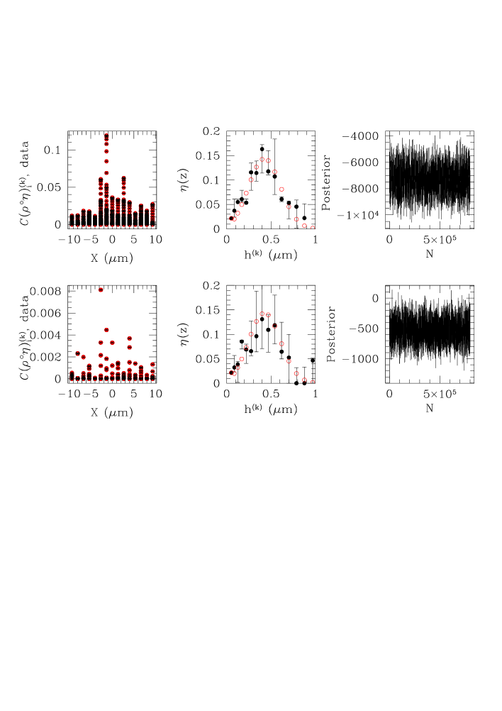
Figure 6: Left: - projection ${\cal C}({\hat{\rho}}\ast{\hat{\eta}})_{i}^{(k)}$ plotted in black, in model units, as a function of beam location on the $X$-axis, (where the beam pointing index $i=1,\ldots,225$), over the image data (in red), for all beam energy values $\epsilon_{k}=2+k$ (in kiloVolts), $k=1,\ldots,18$, for Sample I-CuW (upper panel) and Sample II-CuW with the relatively sparser material density (lower). Middle: estimated correction function, in black, superimposed on the true $\eta^{(\cdot)}$ for the two samples (in red). The error bars in the above plots, as well as in all plots that follow, correspond to 95$\%$ highest probability density credible regions, while the medial level of the posterior is marked by a symbol (filled circle). The trace of the joint posterior probability density of the unknown parameters, given the image data is shown in the right panels. The distribution-free model for the correction function was implemented.

9.2 Low resolution, low-${\cal Z}$ system

Distinguished from the last section, in this section we deal with the case of a low atomic number material imaged at coarse or low imaging resolution. In this case, the surface cross-sectional area of an interaction-volume exceeds that of a voxel only for $E=\epsilon_{k}\leq\epsilon_{k_{in}}$, for $k=1,\ldots,k_{in},k_{in+1},\ldots,N_{{\textrm{eng}}}$. The illustration of this case is discussed here for Sample II-NiAl, that is an alloy of Nickel, Aluminium, Tallium, Rhenium; see ?. The average atomic weight of our simulated sample is such that $k_{in}$=13 but the extent of interaction-volumes attained at $E=\epsilon_{k}$ (=$k$+2 kiloVolts) for $k=14,\ldots,18$, is in excess of the image resolution 1.33 $\mu$m. All other details are as in the previous illustration.

Figure 7 depicts the learnt density structure; visualisation to this effect is provided for the Ni-Al alloy sample in terms of the plots of $\xi_{i}^{(k)}$ against $h^{(k)}$, at chosen values of $X$ and $Y$ inside the sample. Since there are 225 voxels used in these exercises, the depiction of the density at each of these voxels cannot be accommodated in the paper, but Figure 7 shows the density structure at values of beam pointing index $i$ corresponding to 15 values of $Y$, at one value of the $X$ (=6.67$\mu$m).

Figure 7: For the simulated (sparse and low-${\cal Z}$) Sample II-NiAl, the estimated density parameters $\xi_{i}^{(k)}$ plotted in model units as a function of $h^{(k)}$ (in $\mu$m), at $X=6.67$$\mu$m and distinct values of the beam pointing locations along the $Y$-axis, in the range of -10$\mu$m to 10$\mu$m, at intervals of 1.33$\mu$m where the panel in the lower left-hand corner is at the smallest value of $Y$ and that in the upper right-hand most panel is at the highest value of $Y$. The true variation of the learnt material density with depth is shown in red in each panel. This is compared to the material density estimated at the lower and upper bounds of the 95$\%$ HPD credible region, as plotted in cyan and black respectively (in model units). The parametric model for $\eta^{(\cdot)}$ was used.

9.3 High resolution

The challenge posed by the high resolution ($\omega\lesssim$10 nm=0.01 $\mu$m) of imaging, to our modelling is logistical. This logistical problem lies in fact that for $\omega\lesssim$10 nm the run-time involved in the reconstruction of the density over the length scales of $\sim$1 $\mu$m, is prohibitive; for an image resolution of $\omega$=10 nm, there are 100 voxels included over a length interval of 1 $\mu$m, while at example lower resoutions relevant to the aforementioned illustrations there would be ${\mbox{int}}(100/15)$.

In light of this problem, for a high resolution of $\omega$=2 nm that we work with, we choose 20 voxels (each of cross-sectional size 2 nm), across the $X$ range of -20 nm to 20 nm. A similar range in $Y$ is considered. The simulated system is imaged at 10 energy values $\epsilon_{k}=k+1.5$kV, $k=1,\ldots,10$. The atomic number parameter ${\cal Z}$ of the used material is such that the radius $R0^{(1)}=h^{(1)}$ of the interaction-volume attained at $k=1$ is about 21 nm, so that all the studied voxels live inside this and all other (larger) interaction-volumes. It is possible to run multiple parallel chains with data from distinct parts of the observed image, in order to cover this available image. That way, the material density function of the whole sample will be learnt.

The plots of the learnt density for the intrinsically dense and sparse true density functions are shown as a function of depth $Z$, for all $X$ and $Y$, in Fig 8, which display results of runs done with the distribution-free as well as parametric models for the correction function (using $\sigma_{i}^{(k)}=0.05{\tilde{I}}_{i}^{(k)}$, $i=1,\ldots,N_{{\textrm{data}}}$, $k=1,\ldots,N_{{\textrm{eng}}}$). The multiscale structure of the heterogeneity in these simulated density functions is brought out by presenting the logarithms of the estimated densities parameters alongside the logarithms of the chosen or true density parameters.

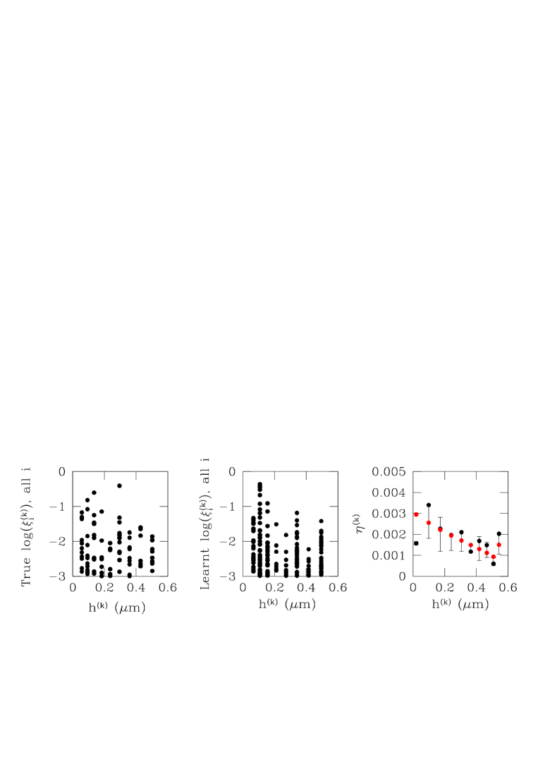
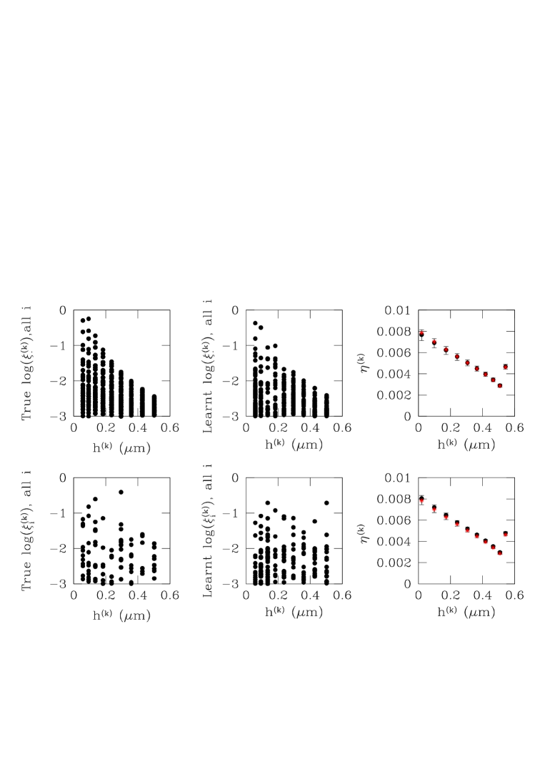
Figure 8: Top row: results of inversion of simulated image data of the intrinsically sparse low-${\cal Z}$ Sample II-NiAl when a distribution-free model for the correction function is used. The true material density structure is presented in the panels on the left, as a function of $z$, for all $X,Y$, in model units. The learnt material density, at the medial level of the posterior, is similarly presented in the middle panels while the learnt $\eta^{(k)}$ over 95$\%$ HPD credible region is shown in black as a function of $h^{(k)}$ in the right panels, in model units, superimposed on the true kernel parameters in red. Middle row: the intrinsically dense, true and learnt (at the posterior median) material density of simulated sample Sample I-NiAl in the left and middle panels respectively with the learnt $\eta^{(\cdot)}$. A parametric model for the correction function is employed. Bottom row: results from implementing simulated images of the sparse Sample II-NiAl when a parametric model for the correction function is employed.

10 Application to the analysis of real SEM image data of Nickel and Silver nano-composite

In this section we discuss the application of the methodology advanced above towards the learning of the 3-D material density and the microscopy correction function (or kernel) by inverting 11 images taken with a real SEM, in a kind of radiation called Back Scattered Electron (BSE). The imaged sample is a brick of Nickel (Ni) and Silver (Ag) nanoparticles, taken with the SEM (the Leica, Stereoscan 430 brand), at 11 distinct values of the beam energy parameter $E$ such that the values that $E$ takes are $10,11,\ldots,20$kV. The brick of nanoparticles was prepared by the drop-cast method in the laboratory. The resolution of BSE imaging with the used SEM is $\approx$50 nm=0.05 $\mu$m, i.e. the smallest length over which sub-structure is depicted in the image is about 50 nm. While this resolution can be coarser than that for images taken in the radiation of Secondary Electrons (?), an image taken in Secondary Electrons will however not bear information coming from the bulk of the material. Hence the motivation behind using BSE image data.

We sample two distinct areas from each of the 2-D images taken at values $10,11,\ldots,20$kV of $E$, resulting in two different image data sets. The first data $D_{1}$ comprises a square area of size 101pixels$\times$101pixels, with this square seated in a different location on an image than the smaller square that contain the pixels that define the image data set $D_{2}$. This second data $D_{2}$ comprises a much smaller square of area 41pixels$\times$41pixels. Given the imaging resolution length of 0.05$\mu$m, i.e. given that the width of each square pixel is 0.05$\mu$m, in image data set $D_{1}$ the 101 pixels along either the $X$ or $Y$-axes are set to accommodate the length interval [-2.5 $\mu$m, 2.5 $\mu$m] while in data $D_{2}$, the pixels occupy the interval [-1 $\mu$m, 1 $\mu$m]. Then in data set $D_{1}$, at a given value of $E$, image datum from a total of 100²=10,000 pixels are recorded, i.e. $N_{{\textrm{data}}}$ for this data set is 10,000. For $D_{2}$, $N_{{\textrm{data}}}$=41²=1,764. Both $D_{1}$ and $D_{2}$ comprise 11 sets of BSE image data $\{{\tilde{I}}_{i}^{(k)}\}_{i=1}^{N_{{\textrm{data}}}}$, with each such set imaged with a beam of energy $\epsilon_{k}$, $k=1,\ldots,11$ such that $\epsilon_{k}=k+9$ kiloVolts. For this material, the mean of the atomic number, atomic mass and physical density in gm cm^-3 yields average atomic number parameter ${\cal Z}$ of 37.5, and the numerical values of the parameters $A$ and $d$ in Equation 3.3 as 83.28 and about 9.7 respectively; then the smallest interacion-volume attained at $E=\epsilon_{1}$ is $R0^{(1)}=h^{(1)}\approx$0.44 $\mu$m and the largest at $E=\epsilon_{10}$ is about 1.4 $\mu$m.

The learning of the material density of a nanostructure is very useful for device engineers engaged in employing such structures in the realisation of electronic devices (?); lack of consistency among measured electronic characteristics of the formed devices is tantamount to deviation from a standardised device behaviour and such can be predicted if heterogeneity in the depth distribution of nanoparticles is identified. Only upon the receipt of quantified information about the latter, is the device engineer able to motivate adequate steps to remedy the device realisation. In addition, such information holds potential to shed light on the physics of interactions between nanoparticles.

If the calibration of the intensity $I_{i}^{(k)}$ of the image datum is available in physical units (of surface density of the BSE), then we could express the measured image data - as manifest in the recorded image - in relevant physical units. In that case, the learnt density could be immediately expressed in physical units. However, such a calibration is not available to us. In fact, in this method, the learnt density is scaled in the following way. The measured value of $\eta^{(1)}$ from microscopy theory (?) for this material suggests using the normalisation factor for $\eta^{(\cdot)}$ is $\approx{\hat{\eta}}^{(1)}/0.325$, so that the $\eta^{(\cdot)}$ parameters, thus normalised, are in the physical units of $\mu$m. (The arithmetic mean of the atomistic parameters of Ni and Ag yield the value of 0.325). This in turn would imply that the material density parameters are each in the physical unit of $\mu$m^-3 since the product of the density and kernel parameters appears in the projection which is measured in physical units of “per unit area”, i.e. in “per length unit²” or ($\mu$m)^-2. Here ${\hat{\eta}}^{(1)}$ is the learnt value of the kernel in the first $Z$-bin. Physically speaking, here we learn the number density in each voxel.

$\begin{array}[]{c c}\includegraphics[width=142.26378pt]{im_10_try1.pdf}&\hskip 14.22636pt\includegraphics[width=142.26378pt]{im_20_try1.pdf}\end{array}$

$\begin{array}[]{c c}\includegraphics[width=156.49014pt,height=213.39566pt]{10_longer.pdf}&\includegraphics[width=156.49014pt,height=213.39566pt]{20_longer.pdf}\end{array}$

Figure 9: The top panels display two of the 11 images of the prepared blend of Nickel and Silver nanoparticles, taken with an SEM, at beam energy values of 20 kV (right) and 10 kV (left). A 5 $\mu$m$\times$ 5 $\mu$m area was identified in each of the 11 images taken in the kind of radiation called Back Scattered Electrons (BSE), to form the data $D_{1}$. The colourised squares in red in each image represent the areas that contribute to $D_{1}$ at energies 20 kV and 10 kV. The distribution of the measured image data over these square areas in red (rotated clockwise by 90^∘), for beam energies of 10 kV and 20 kV are shown in the left and right panels repectively, on the lower row.

The configuration that the constituent nanoparticles are expected to relax into, is due to several factors, including contribution from the surface effects - the surfaces of nanoparticles are active - this encourages interactions, resulting in a clustered configuration. Additionally, gravitational forces that the nanoparticle aggregates sediment under, are also active, with the nanoparticle diameter responsible for determining the relative importance of the different physical influences (?). Thus, in general, along the $Z$-axis, we expect a clustered configuration, embedded within layers. This is what we see in the representation of the learnt density in the $Y=0$ plane, when the image data $D_{1}$ and $D_{2}$ are inverted; see Figure 10. In Figure 11 we present the learnt kernel parameters; the kernels learnt by using data from two distinct parts of the image are expected to overlap given that in our model, the kernel function is a function of $Z$ alone with no dependence on $X$ and $Y$. Such is recovered using data $D_{1}$ and $D_{2}$, as shown in the left panel of this figure. The sequential projections of the convolution of the learnt density and learnt correction function, onto the image space, using the data set $D_{1}$ is overplotted on the image data in Figure 11. The parametric model for the correction function is implemented here.

$\begin{array}[]{c c}\includegraphics[width=170.71652pt]{den_301.pdf}\includegraphics[width=170.71652pt]{den_301_16.pdf}\end{array}$

Figure 10: The left and right panels show the slice of the learnt three dimensional material density in the $Y=0$ plane from inversion of image data $D_{1}$ and $D_{2}$ respectively. In fact, to construct these figures we use the density parameter value that is the median of the posterior of the parameter given the image data. The data are obtained by imaging a brick of Nickel and Silver nanoparticles in a radiation called Back Scattered Electrons, at resolution of 0.05$\mu$m, at 11 different values of $E$, from 10 kV, $\ldots$, 20 kV. $D_{1}$ and $D_{2}$ comprise 101$\times$101 pixels and 41$\times$41 pixels respectively. The labels on the colour-bar are number density values, in physical units (of $\mu$m^-3).

10.1 MCMC convergence diagnostics

In this section we include various diagnostics of an MCMC chain that was run until convergence, using the image data $D_{1}$. These include trace of the likelihood (Figure 12), and histograms of multiple learnt parameters - $\xi_{50}^{(1)}$, $\eta^{(1)}$ - from 1000 steps, in two distinct parts of the chain, namely, for step number $N\in$[1599001,1600000] and $N\in$[799001,800000], respectively (Figure 13). The histograms of the likelihood over these two separate parts of the chain are also presented in this figure.

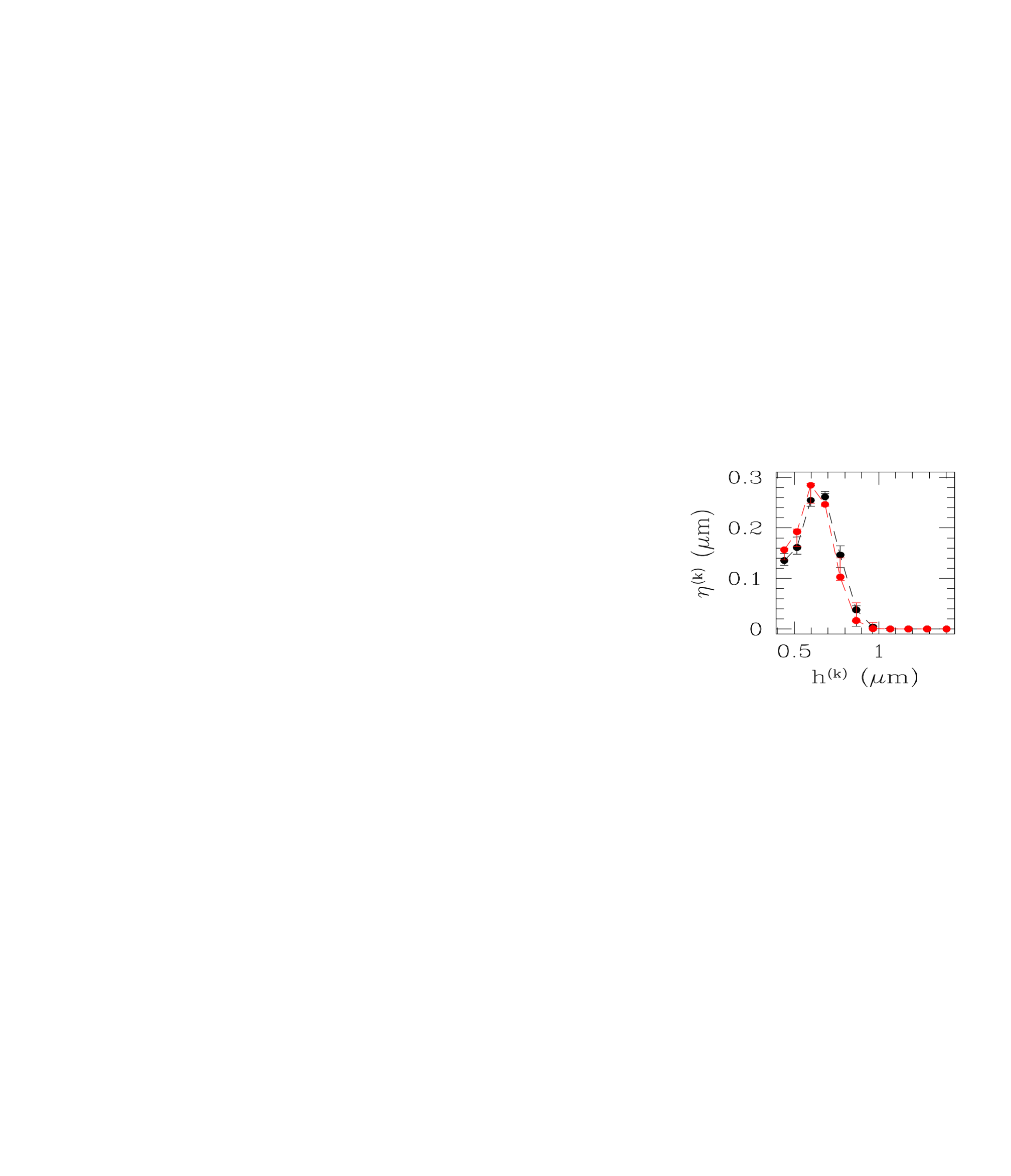
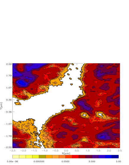
Figure 11: The top panel shows the spatially-averaged projection of convolution of learnt material density and correction function, onto the image space, learnt using image data $D_{1}$ in filled contours. The real image data $D_{1}$ is overlaid in black solid contours. The lower panel shows the correction functions learnt from data $D_{1}$ and $D_{2}$ in black and red respectively. The error bars in this plot represent the learnt 95$\%$ highest probability density region.

$\begin{array}[]{c}\includegraphics[width=227.62204pt]{hist_17.pdf}\end{array}$

Figure 12: The trace of the joint posterior probability density of all uknown model parameters given data $D_{1}$, from a chain that is run with these data.

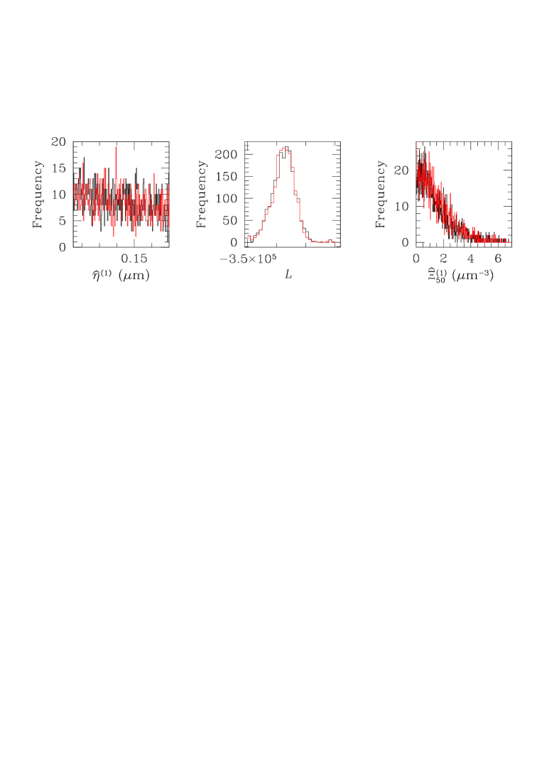
Figure 13: The histograms of the learnt material density in the voxel marked by the viewing vector $\boldsymbol{v}_{i}$, $i=50$ and the lowest value of $E$, ($E=\epsilon_{1}$), from two disjoint parts (middle and end) of the MCMC chain that is 1.6$\times$10⁶ steps long, are depicted in red and black respectively, in the right panel. The histograms of the learnt correction function for $k=1$ , obtained for these two parts of the chain are displayed in the left panel. The histograms of the value of the likelihood in these two parts of the chain are plotted in red and black in the middle panel. The chain was run with real image data $D_{1}$ .

11 Discussion

In this work we have advanced a Bayesian methodology that performs ditribution-free reconstruction of the material density of a material sample and either a parametric or distribution-free reconstruction of the microscopy correction function, given 2-D images of the system taken in any kind of radiation that is generated inside the bulk of the system as a consequence of the material being impinged upon by an electron beam. This methodology is advanced as capable of learning the unknowns even when the the inverse Radon transform is not stable; in addition to noise in the data, such instability can also arise when the underlying distribution of the image data is not continuous. This in turn arises from a material density function that is heterogeneous and is marked by a dense or sparse modal structure, characterised by abruptly declining modal strengths. Given such sharp density contrasts that typify real-life material samples (see Figure 10 and Figure 5), mixture models cannot work satisfactorially in this situation. Also, the density field may not be necessarily convex in real-life material samples. Crucially, this inverse problem connects the measured 2-D radiation in any pixel, with multiple sequential projections of the convolution of the unknown density and the unknown kernel. The novelty of our solution to this harder-than-usual inverse problem includes the imaging of the system at distinct beam energies, adoption of a fully discretised model, identifying priors on the sparsity of the density and borrowing existing knowledge from the domain of application. In this application in which images are taken with electron microscopes, the kernel is the microscopy correction function, the shapes of which are motivated by the microscopy literature. In particular, there is deterministic information available in the literature about the correction at the surface, allowing for identifiability of the global scales of the unknown material density and correction function.

From the point of view of 3-D structure modelling using images taken with bulk microscopic imaging techniques, (such as Scanning Electron Microscopy, Electron Probe Microscopy), our aim here supercedes mere identification of the geometrical distribution of the material i.e. the microstructure. In fact, we aim to estimate the very material density at chosen points inside the bulk of the material sample. Conventionally, Monte Carlo simulation studies of microstructure are undertaken; convolution of such simulated microstructure, with a chosen luminosity density function is then advanced as a model for the density. We advance a methodology that is a major improvement upon this. One key advantage of our approach is that estimates of the 3-D material density are derived from non-invasive and nondestructive bulk imaging techniques. This feature sets our approach beyond standard methodology that typically relies on experimental designs involving the etching away of layers of the sample material at specific depths. Though the microstructure, at this depth, can in principle be identified this way, a measure of $\rho(x,y,z)$ is not achievable. That too, only constraints on the microstructure at such specific depths are possible this way, and interpolation between the layers - based on assumptions about the linearity of the microstructure distribution - are questionable in complex real-life material samples. Of course, such a procedure also damages the sample in the process. Thus, the scope of the non-destructive methodology that we advance is superior. An added flexibility of our model is that it allows for the learning of the correction function from the image data.

The expansion of the information is made possible in this work by suggesting multiple images of the same sample taken with radiation characterised by different values of the parameter $E$ that controls the sub-surface depth from which information is carried, to result in the image. Given the differential penetration depths at different values of $E$, the images taken in this way are realisations of the 3-D structure of the sample to different depths. While a number of attempts at density modelling that use multiple viewing angles have been reported in the literature, the imaging of the system at different $E$ is less common. Logistical advantages of imaging with SEM in this way exist over the conventionally undertaken multi-angle imaging. One example of an imaging technique that may appear to share similarity with our strategy of collecting information from contiguous slices at successive values of the depth variable is volume imaging with MRI, i.e. Magnetic Resonance Imaging (?; ?). However, unlike in our imaging method, in this technique, the image data at any such slice is obtained via multiple angle imaging; the imaging parameter whose value is varied to procure the image data is still the viewing angle, except this variation is implemented at each individual slice. In our method, the parameter that is varied is itself the sub-surface depth, achieved by varying the electron beam energy $E$, since depth has a one-to-one correspondence with $E$.

The method that we have discussed above is indeed developed to solve an unconventionally difficult deprojection problem, but the method is equally capable of estimating the unknown density in an integral equation of the 1^st kind - Fredholm or Volterra - and thereby be applied towards density reconstruction in a wide variety of contexts, when image synthesis is possible. The scope of such applications is of course ample, including the identification and quantification of the density of the metallic molecules that have infused into a piece of polymer that is employed for charge storage purposes, degrading the quality of the device as a result, or the learning of the density of a heterogeneous nanostructure leading to increased understanding of lack of robustness of device behaviour, or identification of the distribution of multiple phases of an alloy in the depth of a metallic sample meant to be used in industry and even estimation of density of luminous matter in astronomical objects, viewed with telescopes, at different wavelengths. In fact, in the case of self-emitting systems that are studied in the emitted particles, the problem is simpler, (as in several other applications), since the interaction-volume is not relevant and the integral reduces to the (easier in general) Volterra integral equation of the first kind. In either case, domain-specific details need to be invoked to attain dimensionality reduction.

REFERENCES

- [1]
- [2] [] Arridge, S. R., & Schotland, J. C. (2009), “Optical tomography: forward and inverse problems,” Inverse Problems, 25, 123010.
- [3]
- [4] [] Bertero, M., & Boccacci, P. (1998), Introduction to inverse problems in imaging, : Taylor and Francis.
- [5]
- [6] [] Bishop, T. E., Babacan, S. D., Amizik, B., Katsaggelos, A. K., Chan, T., & Molina, R. (2007), Blind Image Deconvolution: Problem Formulation and Existing Approaches,, in Blind Image Deconvolution: Theory and Applications, eds. P. Campisi, & K. Egiazarian, CRC Press, Taylor and Francis, pp. 1–41.
- [7]
- [8] [] Carreira-Perpiñán, M. A. (2001), Continuous latent variable models for dimensionality reduction and sequential data reconstruction, Doctoral thesis, University of Sheffield.
- [9]
- [10] [] Chakraborty, S. (2008), “Some Applications of Dirac’s Delta Function in Statistics for More Than One Random Variable,” Applications and Applied Mathematics, 3(1), 42–54.
- [11]
- [12] [] Chib, S., & Greenberg, E. (1995), “Understanding the Metropolis-Hastings Algorithm,” The American Statistician, 49(4), 327.
- [13]
- [14] [] Cotter, S., Dashti, M., & Stuart, A. (2010), “Approximation of Bayesian Inverse Problems,” SIAM Journal of Numerical Analysis, 48, 322–345.
- [15]
- [16] [] Davis, G. R., Dowker, S. E. P., Elliott, J. C., Anderson, P., Wassif, H. S., Boyde, A., Goodship, A. E., Stock, S. R., & Ignatiev, K. (2002), “Non-destructive 3D structural studies by X-ray microtomography,” Advances in X-ray Analysis, 45, 485.
- [17]
- [18] [] Donoho, D. L. (2006), “Compressed sensing,” IEEE Trans. Inform. Theory, 52(4), 1289–1306.
- [19]
- [20] [] Donoho, D., & Tanner, J. (2005), “Sparse Nonnegative Solutions of Underdetermined Linear Equations by Linear Programming,” Proceedings of the National Academy of Sciences, 102(27), 9446.
- [21]
- [22] [] Dorn, O., Bertete-Aguirre, H., & Papanicolaou, G. (2008), “Adjoint fields and sensitivities for 3D electromagnetic imaging in isotropic and anisotropic media,” Inverse Problem and Imaging, 1943, 35.
- [23]
- [24] [] D’Souza, N., Beanland, R., Hayward, C., & Dong, H. (2011), “Accuracy of composition measurement using X-ray spectroscopy in precipitate-strengthened alloys: Application to Ni-base superalloys,” Acta Materialia, 59, 1003.
- [25]
- [26] [] Gabrielyan, N., Saranti, K., Manjunatha, K. N., & Paul, S. (2013), “Growth of low temperature silicon nano-structures for electronic and electrical energy generation applications,” Nanoscale Research Letters, 8(1), 1–7.
- [27]
- [28] [] Gilks, W. R., & Roberts, G. O. (1996), Strategies for improving MCMC,, in Markov Chain Monte Carlo in Practice, eds. W. Gilks, S. Richardson, & D. Spiegelhalter, Interdisciplinary Statistics, Chapman and Hall, London, pp. 89–114.
- [29]
- [30] [] Goldstein, J., Newbury, D. E., Joy, D. C., Lyman, C. E., Echlin, P., Lifshin, E., Sawyer, L., & Michael, J. (2003), Scanning Electron Microscopy and X-ray Microanalysis, New York: Springer Science+Business Media.
- [31]
- [32] [] Gouveia, W. P., & Scales, J. A. (1998), “Bayesian seismic waveform inversion: Parameter estimation and uncertainty analysis,” J. of Geophysical Research, 130(B2), 2759.
- [33]
- [34] [] Greenshtein, E., & Park, J. (2009), “Application of non parametric empirical bayes estimation to high dimensional classification,” Journal of Machine Learning Research, 10, 1687–1704.
- [35]
- [36] [] Haario, H., Laine, M., Mira, A., & Saksman, E. (2006), “DRAM: Efficient adaptive MCMC,” Statistics and Computing, 16, 339.
- [37]
- [38] [] Hall, P., & Qui, P. (2007), “Blind deconvolution and deblurring in image analysis,” Statistica Sinica, 17, 1483–1509.
- [39]
- [40] [] Hans, C. (2009), “Bayesian lasso regularisation,” Biometrika, 96(4), 835.
- [41]
- [42] [] Heinrich, K. F. J., & Newbury, D. E. (1991), Electron probe quantitation, New York: Springer.
- [43]
- [44] [] Helgason, S. (1999), The Radon transform, Progress in Mathematics, Boston: Birkhauser.
- [45]
- [46] [] Hornak, J. P. (1996), “The Basics of MRI,”. http://www.cis.rit.edu/htbooks/mri/.
- [47]
- [48] [] Johnstone, I. M., & Silverman, B. W. (2004), “Needles and straw in haystacks: Empirical Bayes estimates of possibly sparse sequences,” The Annals of Statistics, 32(4), 1594–1649.
- [49]
- [50] [] Joly-Puttez, L. (2011), Tribology of Nanoparticles,, in Handbook of Nanohysics, Nanoparticles and Quantum Dots, ed. e. K. D. Sattler, CRC Press, Taylor and Francis, pp. 26–1.
- [51]
- [52] [] Kanaya, K., & Okamaya, S. (1972)Jl. of Physics D., Applied Physics, 5, 43.
- [53]
- [54] [] Kutchment, P. (2006), Generalised Transforms of the Radon Type and their Applications,, in The Radon Transform, Inverse Problems, and Tomography, eds. G. Olafsson, & e. E. T. Quinto, Vol. 63, American Mathematical society, p. 67.
- [55]
- [56] [] Lee, R. E. (1993), Scanning electron microscopy and X-ray microanalysis, New Jersey, USA: Prentice-Hall.
- [57]
- [58] [] Leone, F., Nottingham, R. B., & Nelson, L. S. (1961), “The Folded Normal Distribution,” Technometrics, 3(4), 543.
- [59]
- [60] [] Li, L., & Speed, T. (2000), “Parametric deconvolution of positive spike trains,” Annals of Statistics, 28, 1270.
- [61]
- [62] [] Markoe, A., & Quinto, E. T. (1985), “An Elementary Proof of Local Invertibility for Generalized and Attenuated Radon Transforms,” SIAM J. Math. Anal., 16, 1114.
- [63]
- [64] [] Mayer, K., Chinta, P. K., Langenberg, K., & Krause, M. (2012), Ultrasonic Imaging of Defects in Known Anisotropic and Inhomogeneous Structures with Fast Synthetic Aperture Methods,, in Proceedings of the 18th World Conference on Non-Destructive Testing, Durban, South Africa, Available online at http://www.ndt.net/article/wcndt2012/toc.htm.
- [65]
- [66] [] Merlet., C. (1994), “An Accurate Computer Correction Program for Quantitative Electron Probe Microanalysis,” Mikrochim. Acta, 114/115, 363.
- [67]
- [68] [] Natterer, F., & Wübbeling, F. (2001), Mathematical methods in image reconstruction, Philadelphia: SIAM.
- [69]
- [70] [] Neal, R. (1998), Regression and Classification Using Gaussian Process Priors,, in Bayesian Statistics 6, eds. J. M. Bernardo, J. O. Berger, A. P. Dawid, & A. F. M. Smith, Oxford University Press, pp. 475–501.
- [71]
- [72] [] Paciorek, C. J., & Schervish, M. (2006), “Spatial modelling using a new class of nonstationary covariance functions,” Environmetrics, 17, 483–506.
- [73]
- [74] [] Panaretos, V. M. (2009), “On Random Tomography with Unobservable Projection Angles,” Annals of Statistics, 37(6), 3272.
- [75]
- [76] [] Park, T., & Casella, G. (2008), “The bayesian lasso,” Journal of the American Statistical Association, 482, 681.
- [77]
- [78] [] Pouchou, J. L., & Pichoir, F. (1984), PAP (Z) procedure for improved quantitative microanalysis, Microbeam Analysis, ed. J.T.Armstrong, San Francisco, California: San Francisco Press.
- [79]
- [80] [] Prasad, P. V. (2006), Magnetic Resonance Imaging: Methods and Biologic Applications, New Jersey: Humana Press Inc.
- [81]
- [82] [] Qui, P. (2008), “A nonparametric procedure for blind image deblurring,” Computational Statistics and Data Analysis, 52, 4828–4842.
- [83]
- [84] [] Reed, S. J. B. (2005), Electron Microprobe Analysis and Scanning Electron Microscopy in Geology, Cambridge: Cambridge University Press.
- [85]
- [86] [] Rullgård, H. (2004), “Stability of the inverse problem for the attenuated Radon transform with 180° data,” Inverse Problems, 20, 781.
- [87]
- [88] [] Sawyer, L., Grubb, D. T., & Meyers, G. F. (2008), Polymer Microscopy, New York: Springer Science.
- [89]
- [90] [] Stuart, A. (2010), “Inverse problems: a Bayesian perspective,” in Acta Numerica, Vol. 19 Cambridge University Press, p. 451.
- [91]
- [92] [] Tarantola, A. (2004), Inverse Problem Theory and Methods for Model Parameter Estimation, Philadelphia: SIAM.
- [93]
- [94] [] Tricomi, F. G. (1985), Integral Equations, New York: Dover Publications.
- [95]
- [96] [] Vanderlinde, W. E., & Caron, J. N. (2007), Blind Deconvolution of SEM Images,, in ISTFA 2007 Conference Proceedings of the 33rd International Symposium for Testing and Failure Analysis, ASM International, pp. 97–102.
- [97]
- [98] [] Wright, J., Yang, A., Ganesh, A., Sastry, S., & Ma, Y. (2009), “Robust Face Recognition via Sparse Representation, and its online supplementary material,” IEEE Transactions on Pattern Analysis and Machine Intelligence (PAMI), 31(2).
- [99]