Space time symmetry in quantum mechanics

Abstract

New prescription to treat position and time equally in quantum mechanics is presented. Using this prescription, we could successfully derive some interesting formulae such as time-of-arrival for a free particle and quantum tunneling formula. The physical interpretation will be discussed.

I Introduction

Though we can treat time and space symmetric way in relativity, in quantum mechanics the time seems different to other observables: It seems we don’t have proper operator for time. A particle detected at one position can be detected at the same position at later time, namely, we encounter the difficulty on orthogonality and normalization and these two measurements do not commute each other. This non commuting property leads us to think about time-of-arrival which means the time that a particle first arrives to a specific position.

Allcock allcock tried to build time-of-arrival eigenstates which are orthogonal each other for different time but could not define a consistent time-of-arrival. His study says that because we cannot absorb the particle in an arbitrarily short time, we cannot measure the time-of-arrival at any accuracy. Oppenheim et alunruh insist that using two level detector absorbing a particle in arbitrarily short period time, we can overcome this restrictions. However they found that the limitation on measuring the time-of-arrival with arbitrarily accuracy comes from the clock coupled to the trigger. They show that if we couple the system to a clock to measure the time-of-arrival at which the particle arrives at specific position, then the accuracy of measurement is limited by

$$\delta t_{A}>\hbar/E_{k}$$

where $\delta t_{A}$ is the minimum uncertainty of measuring time of arrival and $E_{k}$ is the energy of clock.

One of interesting approaches to find the time-of-arrival operator has been studied by Grot et al.grot They tried to develop the time-of-arrival operator for free non-relativistic particle by proper ordering of space time operator in Heisenberg picture, analogous to classical picture. But the eigenstates of time-of-arrival they calculated satisfying eigenvalue equation, did not satisfy the orthogonal condition for different times. They bypassed this difficulty by modifying the time-of-arrival operator so that in the classical limit would not reproduced the time-of-arrival exactly, but would reproduce a quantity arbitrary close to the time-of-arrival.

In this article, I will not attempt to develop the time-of-arrival operator nor discuss about dynamical limitation on treating position and time of quantum mechanics in equal manner. Rather it will be focused on how we can put an equal footing on position and time in quantum mechanical evolution. Contrast to other approaches, I assumed that we cannot put an equal footing on both position and time simultaneously. That is, when we treat the position as a quantum operator, we have to treat the time as an evolution parameter. And when we treat the time as a quantum operator, we have to treat the position as an evolution parameter. We will discuss how we can apply this prescription on quantum tunneling process.

II Prescription

In this section notational conventions will be defined in symmetrical way for both position and time. When the time is used as an evolution parameter (TEP), the position is used as a usual quantum observable. When the position is used as an evolution parameter (PEP), the time is used as a usual quantum observable. We can specify any quantum states with one state vector and one evolution parameter.

II.1 TEP

We denote the quantum state $\psi$ at time $t_{1}$ by

$$\mid\psi,\underline{t_{1}}\rangle$$ (1)

where the underline on $\underline{t_{1}}$ means that time is the evolution parameter. That is, the first one represents the quantum state and the second one stands for the evolution parameter. We can express (1) it shorter by

$$\mid\psi_{1}\rangle\equiv\mid\psi,\underline{t_{1}}\rangle$$ (2)

where the subscript 1 on $\psi$ means the state is of time $t_{1}$. The probability amplitude to find the position $x$ is then

$$\langle x\mid\psi,\underline{t_{1}}\rangle=\psi(x,\underline{t_{1}})$$ (3)

where the position $x$ is the usual quantum observable and the time $\underline{t_{1}}$ is the evolution parameter. Thus while the operation $\langle x\mid x_{1}\rangle$ is possible, the operation $\langle\underline{t}\mid\underline{t_{1}}\rangle$ is not possible because both $t$ and $t_{1}$ are just evolution parameters. By the same reason $\langle\underline{t}\mid\psi,\underline{t_{1}}\rangle=\psi(\underline{t},\underline{t_{1}})$ does not make sense. Since this represents the pure evolution process up to $t$, it must be denoted by

$$\langle\underline{t}\mid\psi,\underline{t_{1}}\rangle=\mid\psi,\underline{t}\rangle$$ (4)

II.2 PEP

We denote the quantum state $\varphi$ at position $x_{1}$ by

$$\mid\varphi,\underline{x_{1}}\rangle$$ (5)

where the underline on $\underline{x_{1}}$ means that position is the evolution parameter. That is, the first one represents the quantum state and the second one stands for the evolution parameter. We can express (5) it shorter by

$$\mid\varphi_{1}\rangle\equiv\mid\varphi,\underline{x_{1}}\rangle$$ (6)

where the subscript 1 on $\varphi$ means the state is of position $x_{1}$. The probability amplitude to find the time $t$ is then

$$\langle t\mid\varphi,\underline{x_{1}}\rangle=\varphi(t,\underline{x_{1}})$$ (7)

where the time $t$ is the usual quantum observable and the position $\underline{x_{1}}$ is the evolution parameter. Thus while the operation $\langle t\mid t_{1}\rangle$ is possible, the operation $\langle\underline{x}\mid\underline{x_{1}}\rangle$ is not possible because both $x$ and $x_{1}$ are just evolution parameters. By the same reason $\langle\underline{x}\mid\varphi,\underline{x_{1}}\rangle=\varphi(\underline{x},\underline{x_{1}})$ does not make sense. Since this represents the pure evolution process up to $x$, it must be denoted by

$$\langle\underline{x}\mid\varphi,\underline{x_{1}}\rangle=\mid\varphi,\underline{x}\rangle$$ (8)

As we have seen, any quantum state is expressed by one state vector and one evolution parameter as $\mid\psi,\underline{t}\rangle$ or $\mid\varphi,\underline{x}\rangle$. We cannot specify a quantum state by $\mid\psi,x,\underline{t}\rangle$ (two state vectors) or by $\mid\psi,\underline{x},\underline{t}\rangle$ (two evolution parameters).

The rule is simple: The state vector $\psi$ does not operate to the evolution parameter $\underline{e}$. So $\langle\underline{e}\mid\psi\rangle$ does not work. Only two exceptions are $\langle\underline{t}\mid E_{n}\rangle=e^{-iE_{n}t}$ and $\langle\underline{x}\mid p_{n}\rangle=e^{ip_{n}x}$ where $E_{n}$, $p_{n}$ are the components of identity operator $I=\sum_{n}\mid p_{n}\rangle\langle p_{n}\mid=\sum_{n}\mid E_{n}\rangle\langle E_{n}\mid$. If $E$ is not a component of identity operator and $\langle\underline{t}\mid E\rangle=e^{-iEt}$ contributes only overall phase, then it is physically meaningless.

And two state vectors with different evolution parameters do not directly operate each other. For example, two state vectors $\varphi$ and $\psi$ in $\langle\varphi,\underline{t_{2}}\mid\psi,\underline{t_{1}}\rangle$ do not directly operate each other. In this case, if needed, we may sandwich

$$I=\sum_{n}\mid E_{n}\rangle\langle E_{n}\mid$$ (9)

between $\underline{t_{2}}$ and $\underline{t_{1}}$ or we may sandwich

$$I=\sum_{n}\mid p_{n}\rangle\langle p_{n}\mid$$ (10)

between $\underline{x_{2}}$ and $\underline{x_{1}}$.

III Expression in $E$ and $p$ basis

III.1 TEP

We can express the quantum state $\psi$ at time $t_{1}$ by

$$\mid\psi_{1},\underline{t_{1}}\rangle=\mid E_{n}\rangle\langle E_{n}\mid\psi_{1},\underline{t_{1}}\rangle$$ (11)

where the summation is assumed for repeated index $n$. Thus the probability amplitude to find the state $\psi_{2}$ at $t_{2}$ is

$$\langle\psi_{2},\underline{t_{2}}\mid\psi_{1},\underline{t_{1}}\rangle=\langle\psi_{2},\underline{t_{2}}\mid E_{n}\rangle\langle E_{n}\mid\psi_{1},\underline{t_{1}}\rangle$$ (12)

For example, $\psi_{2}=x_{2}$,

$$\langle x_{2},\underline{t_{2}}\mid\psi_{1},\underline{t_{1}}\rangle = \langle x_{2},\underline{t_{2}}\mid E_{n}\rangle\langle E_{n}\mid\psi_{1},\underline{t_{1}}\rangle$$

$$\langle x_{2}\mid\psi_{2},\underline{t_{2}}\rangle = \langle x_{2}\mid E_{n}\rangle\langle\underline{t_{2}}\mid E_{n}\rangle\langle E_{n}\mid\psi_{1}\rangle\langle E_{n}\mid\underline{t_{1}}\rangle$$

$$\to\psi_{2}(x_{2},\underline{t_{2}}) = \int\langle x_{2}\mid E\rangle\psi_{1}(E)e^{-iE(t_{2}-t_{1})}{dE}$$

where the subscripts 1 and 2 in $\psi$ mean the states $\psi$ is of $t_{1}$ and $t_{2}$, we set $\hbar=1$.

III.2 PEP

We can express the quantum state $\varphi$ at position $x_{1}$ by

$$\mid\varphi_{1},\underline{x_{1}}\rangle=\mid p_{n}\rangle\langle p_{n}\mid\varphi_{1},\underline{x_{1}}\rangle$$ (13)

The probability amplitude to find the state $\varphi_{2}$ at $x_{2}$ is

$$\langle\varphi_{2},\underline{x_{2}}\mid\varphi_{1},\underline{x_{1}}\rangle=\langle\varphi_{2},\underline{x_{2}}\mid p_{n}\rangle\langle p_{n}\mid\varphi_{1},\underline{x_{1}}\rangle$$ (14)

For example, $\varphi_{2}=t_{2}$,

$$\langle t_{2},\underline{x_{2}}\mid\varphi_{1},\underline{x_{1}}\rangle = \langle t_{2},\underline{x_{2}}\mid p_{n}\rangle\langle p_{n}\mid\varphi_{1},\underline{x_{1}}\rangle$$

$$\langle t_{2}\mid\varphi_{2},\underline{x_{2}}\rangle = \langle t_{2}\mid p_{n}\rangle\langle\underline{x_{2}}\mid p_{n}\rangle\langle p_{n}\mid\varphi_{1}\rangle\langle p_{n}\mid\underline{x_{1}}\rangle$$

$$\to\varphi_{2}(t_{2},\underline{x_{2}}) = \int\langle t_{2}\mid p\rangle\varphi_{1}(p)e^{ip(x_{2}-x_{1})}dp$$ (15)

IV Expression in space time basis

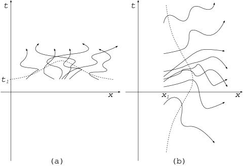
Figure 1: (a) Illustration of (17); (b) Illustration of (20)

IV.1 TEP

In (11) and (12), let’s use $\mid x_{i},\underline{t_{1}}\rangle\langle x_{i},\underline{t_{1}}\mid$ instead of $\mid E_{n}\rangle\langle E_{n}\mid$.

$$\mid\psi_{1},\underline{t_{1}}\rangle = \mid x_{i},\underline{t_{1}}\rangle\langle x_{i},\underline{t_{1}}\mid\psi_{1},\underline{t_{1}}\rangle=\int\mid x,\underline{t_{1}}\rangle\langle x\mid\psi_{1}\rangle dx$$ (16)

$$= \int\mid x,\underline{t_{1}}\rangle\langle x\mid p_{n}\rangle\langle p_{n}\mid\psi_{1}\rangle dx=\int\mid x,\underline{t_{1}}\rangle\frac{e^{ip_{n}x}}{\sqrt{2\pi}}\langle p_{n}\mid\psi_{1}\rangle dx$$ (17)

For the momentum eigenstate $\psi_{1}=p_{1}$,

$$\mid p_{1},\underline{t_{1}}\rangle=\int\mid x,\underline{t_{1}}\rangle\frac{e^{ip_{1}x}}{\sqrt{2\pi}}dx$$ (18)

From (18), we can see that a particle in momentum eigenstate evolving from time $\underline{t_{1}}$ starts its motion at all equally different positions. (17) is illustrated in figure 1(a). We can check that if we are more certain about the momentum of a particle, we are less certain about the position of departure at time $\underline{t_{1}}$. This is the fundamental meaning of position-momentum uncertainty relation.

IV.2 PEP

In (13) and (14), let’s use $\mid t_{i},\underline{x_{1}}\rangle\langle t_{i},\underline{x_{1}}\mid$ instead of $\mid p_{n}\rangle\langle p_{n}\mid$.

$$\mid\varphi_{1},\underline{x_{1}}\rangle = \mid t_{i},\underline{x_{1}}\rangle\langle t_{i},\underline{x_{1}}\mid\varphi_{1},\underline{x_{1}}\rangle=\int\mid t,\underline{x_{1}}\rangle\langle t\mid\varphi_{1}\rangle dt$$ (19)

$$= \int\mid t,\underline{x_{1}}\rangle\langle t\mid E_{n}\rangle\langle E_{n}\mid\varphi_{1}\rangle dt=\int\mid t,\underline{x_{1}}\rangle\frac{e^{-iE_{n}t}}{\sqrt{2\pi}}\langle E_{n}\mid\varphi_{1}\rangle dt$$ (20)

For the energy eigenstate $\varphi_{1}=E_{1}$,

$$\mid E_{1},\underline{x_{1}}\rangle=\int\mid t,\underline{x_{1}}\rangle\frac{-e^{iE_{1}t}}{\sqrt{2\pi}}dt$$ (21)

From (21), we can see that the particle in energy eigenstate evolving from the position $\underline{x_{1}}$ starts its motion at all equally different times. (20) is illustrated in figure 1(b). We can check that if we are more certain about the energy of a particle, we are less certain about the time of departure at position $\underline{x_{1}}$. This is the fundamental meaning of time-energy uncertainty relation.

V Quantum evolution in space time basis

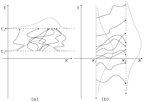
Figure 2: (a) Illustration of (22); (b) Illustration of (27)

V.1 TEP

Let’s find the expression for the probability amplitude of quantum state $\psi_{1}$ at $\underline{t_{1}}$ to be measured $\psi_{2}$ at $\underline{t_{2}}$.

$$\langle\psi_{2},\underline{t_{2}}\mid\psi_{1},\underline{t_{1}}\rangle = \int\underbrace{\langle\psi_{2},\underline{t_{2}}\mid x_{2},\underline{t_{2}}\rangle}_{\langle\psi_{2}\mid x_{2}\rangle}\langle x_{2},\underline{t_{2}}\mid x_{1},\underline{t_{1}}\rangle\underbrace{\langle x_{1},\underline{t_{1}}\mid\psi_{1},\underline{t_{1}}\rangle}_{\langle x_{1}\mid\psi_{1}\rangle}dx_{1}dx_{2}$$ (22)

$$= \iint\langle\psi_{2}\mid x_{2}\rangle\langle x_{2},\underline{t_{2}}\mid x_{1},\underline{t_{1}}\rangle\langle x_{1}\mid\psi_{1}\rangle dx_{1}dx_{2}$$

Equation (22) is illustrated in figure 2(a).

For example

$$\langle x_{2},\underline{t_{2}}\mid\psi,\underline{t_{1}}\rangle = \iint\langle x_{2}\mid x_{2}^{\prime}\rangle\langle x_{2}^{\prime},\underline{t_{2}}\mid x_{1},\underline{t_{1}}\rangle\langle x_{1}\mid\psi_{1}\rangle dx_{1}dx_{2}^{\prime}$$ (23)

$$\langle x_{2}\mid\psi,\underline{t_{2}}\rangle = \int\langle x_{2},\underline{t_{2}}\mid x_{1},\underline{t_{1}}\rangle\langle x_{1}\mid\psi_{1}\rangle dx_{1}$$ (24)

$$\to\psi(x_{2},\underline{t_{2}}) = \int\langle x_{2},\underline{t_{2}}\mid x_{1},\underline{t_{1}}\rangle\psi(x_{1},\underline{t_{1}})dx_{1}$$ (25)

Take an another example

$$\langle p_{2},\underline{t_{2}}\mid p_{1},\underline{t_{1}}\rangle =\iint\langle p_{2}\mid x_{2}\rangle\langle x_{2},\underline{t_{2}}\mid x_{1},\underline{t_{1}}\rangle\langle x_{1}\mid p_{1}\rangle dx_{1}dx_{2}$$

$$=\iint\frac{e^{-ip_{2}x_{2}}}{\sqrt{2\pi}}\langle x_{2},\underline{t_{2}}\mid x_{1},\underline{t_{1}}\rangle\frac{e^{ip_{1}x_{1}}}{\sqrt{2\pi}}dx_{1}dx_{2}$$ (26)

V.2 PEP

Let’s find the expression for the probability amplitude of quantum state $\varphi_{1}$ at $\underline{x_{1}}$ to be measured $\varphi_{2}$ at $\underline{x_{2}}$.

$$\langle\varphi_{2},\underline{x_{2}}\mid\varphi_{1},\underline{x_{1}}\rangle = \int\underbrace{\langle\varphi_{2},\underline{x_{2}}\mid t_{2},\underline{x_{2}}\rangle}_{\langle\varphi_{2}\mid t_{2}\rangle}\langle t_{2},\underline{x_{2}}\mid t_{1},\underline{x_{1}}\rangle\underbrace{\langle t_{1},\underline{x_{1}}\mid\varphi_{1},\underline{x_{1}}\rangle}_{\langle t_{1}\mid\varphi_{1}\rangle}dt_{1}dt_{2}$$ (27)

$$= \iint\langle\varphi_{2}\mid t_{2}\rangle\langle t_{2},\underline{x_{2}}\mid t_{1},\underline{x_{1}}\rangle\langle t_{1}\mid\varphi_{1}\rangle dt_{1}dt_{2}$$

Equation (27) is illustrated in figure 2(b).

For example

$$\langle t_{2},\underline{x_{2}}\mid\varphi,\underline{x_{1}}\rangle = \iint\langle t_{2}\mid t_{2}^{\prime}\rangle\langle t_{2}^{\prime},\underline{x_{2}}\mid t_{1},\underline{x_{1}}\rangle\langle t_{1}\mid\varphi_{1}\rangle dt_{1}dt_{2}^{\prime}$$ (28)

$$\langle t_{2}\mid\varphi,\underline{x_{2}}\rangle = \int\langle t_{2},\underline{x_{2}}\mid t_{1},\underline{x_{1}}\rangle\langle t_{1}\mid\varphi_{1}\rangle dt_{1}$$ (29)

$$\to\varphi(t_{2},\underline{x_{2}}) = \int\langle t_{2},\underline{x_{2}}\mid t_{1},\underline{x_{1}}\rangle\varphi(t_{1},\underline{x_{1}})dt_{1}$$ (30)

Take an another example

$$\langle E_{2},\underline{x_{2}}\mid E_{1},\underline{x_{1}}\rangle =\iint\langle E_{2}\mid t_{2}\rangle\langle t_{2},\underline{x_{2}}\mid t_{1},\underline{x_{1}}\rangle\langle t_{1}\mid E_{1}\rangle dt_{1}dt_{2}$$

$$=\iint\frac{e^{iE_{2}t_{2}}}{\sqrt{2\pi}}\langle t_{2},\underline{x_{2}}\mid t_{1},\underline{x_{1}}\rangle\frac{e^{-iE_{1}t_{1}}}{\sqrt{2\pi}}dt_{1}dt_{2}$$ (31)

VI Orthogonality of position and time

In this section it will be shown how to achieve $\langle\>x\mid x^{\prime}\>\rangle=\delta(x-x^{\prime})$ in TEP and $\langle\>t\mid t^{\prime}\>\rangle=\delta(t-t^{\prime})$ in PEP. In doing so, we will find the following expression for $\langle\>E\mid p\>\rangle$.

$$\langle\>E\mid p\>\rangle=\sqrt{\frac{E}{p_{E}}}\delta(\pm p_{E}-p)\qquad\textrm{in TEP}$$ (32)

The range of energy is either $[m,\infty]$ or $[-m,-\infty]$. The range of momentum is $[-\infty,\infty]$.

$$\langle\>E\mid p\>\rangle=\sqrt{\frac{p}{E_{p}}}\delta(\pm E_{p}-E)\qquad\textrm{in PEP}$$ (33)

The range of momentum is either $[0,\infty]$ or $[0,-\infty]$. The range of energy is $[-\infty,\infty]$ except $[-m,m]$. Where $p_{E}\equiv\sqrt{E^{2}-m^{2}}$ and $E_{p}\equiv\sqrt{p^{2}+m^{2}}$ for a free particle. Let’s check this out.

VI.1 TEP

In order to find out the expression of $\langle\>E\mid p\>\rangle$, first verify the orthogonality of momentum, $\langle\>p^{\prime}\mid p\>\rangle=\int\langle\>p^{\prime}\mid E\>\rangle\langle\>E\mid p\>\rangle dE=\delta(p^{\prime}-p)$. Since $EdE=p_{E}dp_{E}$, try $\langle\>E\mid p\>\rangle=\sqrt{E/p_{E}}\delta(\pm p_{E}-p)$, where $\pm$ indicates that when we integrate over $p_{E}$, we have to do it for both $+p_{E}$ and $-p_{E}$.

$$\langle\>p^{\prime}\mid p\>\rangle=\int\sqrt{\frac{E}{p_{E}}}\delta(\pm p_{E}-p^{\prime})\sqrt{\frac{E}{p_{E}}}\delta(\pm p_{E}-p)dE$$ (34)

This is an odd function of $E$, thus if we integrate over $[-\infty,\infty]$, it turns out to be zero. We can fix it by restricting $E$ to either $[m,\infty]$ or $[-m,-\infty]$. Then,

$$\langle\>p^{\prime}\mid p\>\rangle=\int^{\infty}_{m}\frac{E}{p_{E}}\delta(\pm p_{E}-p^{\prime})\delta(\pm p_{E}-p)dE$$ (35)

The sign of $E$ does not specify the sign of $p_{E}$. Thus we have to count both positive and negative momentum cases.

$$\langle\>p^{\prime}\mid p\>\rangle =\int^{\infty}_{0}\delta(p_{E}-p^{\prime})\delta(p_{E}-p)dp_{E}+\int^{\infty}_{0}\delta(p_{E}+p^{\prime})\delta(p_{E}+p)dp_{E}$$ (36)

$$=\int^{\infty}_{0}\delta(p_{E}-p^{\prime})\delta(p_{E}-p)dp_{E}+\int^{-\infty}_{0}\delta(-u+p^{\prime})\delta(-u+p)d(-u)$$ (37)

$$=\int^{\infty}_{-\infty}\delta(p_{E}-p^{\prime})\delta(p_{E}-p)dp_{E}=\delta(p^{\prime}-p)$$ (38)

(32) with $E$ either $[m,\infty]$ or $[-m,-\infty]$ ensures the orthogonality of position, $\langle\>x\mid x^{\prime}\>\rangle=\delta(x-x^{\prime})$:

$$\langle\>x\mid E\>\rangle=\int\langle\>x\mid p\>\rangle\langle\>p\mid E\>\rangle dp=\frac{1}{\sqrt{2\pi}}\int e^{ipx}\sqrt{\frac{E}{p_{E}}}\delta(\pm p_{E}-p)dp=\frac{1}{\sqrt{2\pi}}\sqrt{\frac{E}{p_{E}}}e^{\pm ip_{E}x}$$ (39)

$$\langle\>x\mid x^{\prime}\>\rangle =\int^{\infty}_{m}\langle\>x\mid E\>\rangle\langle\>E\mid x^{\prime}\>\rangle dE=\frac{1}{2\pi}\int^{\infty}_{m}\frac{E}{p_{E}}e^{\pm ip_{E}(x-x^{\prime})}dE$$ (40)

$$=\frac{1}{2\pi}\int^{\infty}_{-\infty}e^{ip_{E}(x-x^{\prime})}dp_{E}=\delta(x-x^{\prime})$$ (41)

If we did not restrict $E$ to either positive or negative values, we couldn’t have $\langle\>x\mid x^{\prime}\>\rangle=\delta(x-x^{\prime})$. This is expected because the negative energy particle comes backward in time to be detected at another position at the same time it has already been detected.

VI.2 PEP

In order to find out the expression of $\langle\>E\mid p\>\rangle$, first verify the orthogonality of energy, $\langle\>E^{\prime}\mid E\>\rangle=\int\langle\>E^{\prime}\mid p\>\rangle\langle\>p\mid E\>\rangle dp=\delta(E^{\prime}-E)$. Since $EdE=p_{E}dp_{E}$, try $\langle\>E\mid p\>\rangle=\sqrt{p/E_{p}}\delta(\pm E_{p}-E)$.

$$\langle\>E^{\prime}\mid E\>\rangle=\int\sqrt{\frac{p}{E_{p}}}\delta(\pm E_{p}-E^{\prime})\sqrt{\frac{p}{E_{p}}}\delta(\pm E_{p}-E)dp$$ (42)

This is an odd function of $p$, thus if we integrate over $[-\infty,\infty]$, it turns out to be zero. We can fix it by restricting $p$ to either $[0,\infty]$ or $[0,-\infty]$. Then,

$$\langle\>E^{\prime}\mid E\>\rangle=\int^{\infty}_{0}\frac{p}{E_{p}}\delta(\pm E_{p}-E^{\prime})\delta(\pm E_{p}-E)dp$$ (43)

The sign of $p$ does not specify the sign of $E_{p}$. Thus we have to count both positive and negative energy cases.

$$\langle\>E^{\prime}\mid E\>\rangle =\int^{\infty}_{0}\delta(E_{p}-E^{\prime})\delta(E_{p}-E)dE_{p}+\int^{\infty}_{0}\delta(E_{p}+E^{\prime})\delta(E_{p}+E)dE_{p}$$ (44)

$$=\int^{\infty}_{0}\delta(E_{p}-E^{\prime})\delta(E_{p}-E)dE_{p}+\int^{-\infty}_{0}\delta(-u+E^{\prime})\delta(-u+E)d(-u)$$ (45)

$$=\int^{\infty}_{-\infty}\delta(E_{p}-E^{\prime})\delta(E_{p}-E)dE_{p}=\delta(E^{\prime}-E)$$ (46)

(33) with $p$ either $[0,\infty]$ or $[0,-\infty]$ ensures the orthogonality of time, $\langle\>t\mid t^{\prime}\>\rangle=\delta(t-t^{\prime})$:

$$\langle\>p\mid t\>\rangle=\int\langle\>p\mid E\>\rangle\langle\>E\mid t\>\rangle dE=\frac{1}{\sqrt{2\pi}}\int\sqrt{\frac{p}{E_{p}}}\delta(\pm E_{p}-E)e^{iEt}dE=\frac{1}{\sqrt{2\pi}}\sqrt{\frac{p}{E_{p}}}e^{\pm iE_{p}t}$$ (47)

$$\langle\>t\mid t^{\prime}\>\rangle =\int^{\infty}_{0}\langle\>t\mid p\>\rangle\langle\>p\mid t^{\prime}\>\rangle dp=\frac{1}{2\pi}\int^{\infty}_{0}\frac{p}{E_{p}}e^{\pm iE_{p}(t^{\prime}-t)}dp$$ (48)

$$=\frac{1}{2\pi}\int^{\infty}_{-\infty}e^{iE_{p}(t^{\prime}-t)}dE_{p}=\delta(t-t^{\prime})$$ (49)

If we did not restrict $p$ to either positive or negative values, we couldn’t have $\langle\>t\mid t^{\prime}\>\rangle=\delta(t-t^{\prime})$. This is expected because the negative momentum particle comes backward in space to be detected at another time at the same position it has already been detected.

VII Application

We have seen how to treat the position and time equally in quantum mechanics especially in evolution process. Let’s consider some application of our prescrition.

VII.1 Time-of-arrival

We may apply new prescription to the time-of-arrival introduced earlier. By putting (47) into (15), we can derive the expression of time-of-arrival for a free particle. Then (15) turns out

$$\varphi_{2}(t)=\frac{1}{\sqrt{2\pi}}\int\sqrt{\frac{p}{E_{p}}}e^{\mp iE_{p}t+ip(x_{2}-x_{1})}\varphi_{1}(p)dp$$ (50)

where the subscript 1 and 2 in $\varphi$ stands for the position $x_{1}$ and $x_{2}$. The range of $p$ goes either $[0,\infty]$ or $[0,-\infty]$; $\mp E_{p}$ correspond positive and negative energy particle respectively. The negative energy particle evolves in opposite direction to the positive energy particle in time. (50) is well consistent with the final result Grot et algrot derived for a free particle.

We have drived (50) from $\langle\>t_{2},\underline{x_{2}}\mid p_{n}\>\rangle\langle\>p_{n}\mid\varphi_{1},\underline{x_{1}}\>\rangle$. We could also derive (50) from $\langle\>t_{2},\underline{x_{2}}\mid t_{i},\underline{x_{1}}\>\rangle\langle\>t_{i},\underline{x_{1}}\mid\varphi_{1},\underline{x_{1}}\>\rangle$.

$$\langle\>t_{2},\underline{x_{2}}\mid\varphi_{1},\underline{x_{1}}\>\rangle =\int dt_{1}\langle\>t_{2},\underline{x_{2}}\mid t_{1},\underline{x_{1}}\>\rangle\langle\>t_{1},\underline{x_{1}}\mid\varphi_{1},\underline{x_{1}}\>\rangle$$ (51)

$$\langle\>t_{2}\mid\varphi_{2},\underline{x_{2}}\>\rangle =\int dt_{1}\langle\>t_{2},\underline{x_{2}}\mid p_{m}\>\rangle\langle\>p_{m}\mid t_{1},\underline{x_{1}}\>\rangle\langle\>t_{1},\underline{x_{1}}\mid p_{n}\>\rangle\langle\>p_{n}\mid\varphi_{1},\underline{x_{1}}\>\rangle$$ (52)

$$\varphi_{2}(t_{2}) =\int dt_{1}\langle\>t_{2}\mid p_{m}\>\rangle\langle\>p_{m}\mid t_{1}\>\rangle\langle\>\underline{x_{2}}\mid p_{m}\>\rangle\langle\>p_{m}\mid\underline{x_{1}}\>\rangle\langle\>t_{1}\mid p_{n}\>\rangle\langle\>p_{n}\mid\varphi_{1}\>\rangle$$ (53)

$$\varphi_{2}(t_{2}) =\iiint dt_{1}\Big{(}\frac{p_{m}}{2\pi E_{p_{m}}}\Big{)}\sqrt{\frac{p_{n}}{2\pi E_{p_{n}}}}e^{\pm i(E_{p_{m}}-E_{p_{n}})t_{1}}e^{\mp iE_{p_{m}}t_{2}}e^{ip_{m}(x_{2}-x_{1})}\varphi_{1}(p_{n})dp_{m}dp_{n}$$ (54)

$$=\iint\frac{p_{m}}{E_{p_{m}}}\sqrt{\frac{p_{n}}{2\pi E_{p_{n}}}}\delta(E_{p_{m}}-E_{p_{n}})e^{\mp E_{p_{m}}t_{2}+ip_{m}(x_{2}-x_{1})}\varphi_{1}(p_{n})\frac{E_{p_{m}}dE_{p_{m}}}{p_{m}}dp_{n}$$ (55)

$$=\int^{\infty}_{0}\sqrt{\frac{p_{n}}{2\pi E_{p_{n}}}}e^{\mp E_{p_{n}}t_{2}+ip_{n}(x_{2}-x_{1})}\varphi_{1}(p_{n})dp_{n}$$ (56)

which reduce to (50). Note that if we did not restrict the momentum to either $[0,\infty]$ or $[0,-\infty]$, we could not have $e^{ip_{n}(x_{2}-x_{1})}$ in (56) from (55).

VII.2 Quantum tunneling

Another application is the region of quantum tunneling. (Or inside event horizon.) Thus let’s apply the prescription to derive quantum tunneling formula. For $E_{1}=E_{2}$ (31) becomes

$$\langle E_{1},\underline{x_{2}}\mid E_{1},\underline{x_{1}}\rangle =\iint\langle t_{2},\underline{x_{2}}\mid t_{1},\underline{x_{1}}\rangle\frac{1}{2\pi}e^{iE_{1}(t_{2}-t_{1})}dt_{1}dt_{2}$$

$$=\frac{1}{2\pi}\int^{\infty}_{-\infty}\int^{\infty}_{-\infty}\sum_{[x(t)]}\exp\Big{(}i\int^{t_{2}}_{t_{1}}(L+E_{1})dt\Big{)}dt_{1}dt_{2}$$

where we have used Feynman kernal. And we can make it simpler by

$$\int^{t_{2}}_{t_{1}}(L+E_{1})dt=\int^{t_{2}}_{t_{1}}p\dot{x}dt=\int^{x_{2}}_{x_{1}}pdx\equiv W(x)\Big{|}^{x_{2}}_{x_{1}}$$ (57)

where $p\equiv\frac{\partial L}{\partial\dot{x}}$ and $W$ stand for the generalized momentum and the Jacobi action respectively. Then finally we have

$$\langle E_{1},\underline{x_{2}}\mid E_{1},\underline{x_{1}}\rangle=\frac{1}{2\pi}\int^{\infty}_{-\infty}\int^{\infty}_{-\infty}\sum_{[x(t)]}\exp\frac{iW(x)\Big{|}^{x_{2}}_{x_{1}}}{\hbar}dt_{1}dt_{2}$$ (58)

For a classical object ($W\gg\hbar$) or for WKB approximation hibbs ,

$$\sum_{[x(t)]}\exp\Big{(}\frac{iW(x)\Big{|}^{x_{2}}_{x_{1}}}{\hbar}\Big{)}\sim\exp\Big{(}\frac{iW(x_{\ell})\Big{|}^{x_{2}}_{x_{1}}}{\hbar}\Big{)}F(t_{2},t_{1})$$ (59)

where $F(t_{2},t_{1})$ is some function of only $t_{2}$ and $t_{1}$. $x_{\ell}$ stands for the least action path satisfying Euler-Lagrange equation

$$\frac{\partial}{\partial t}\Big{(}\frac{\partial L}{\partial\dot{x}}\Big{)}-\frac{\partial L}{\partial x}=0$$ (60)

Thus

$$\langle E_{1},\underline{x_{2}}\mid E_{1},\underline{x_{1}}\rangle\simeq\exp\Big{(}\frac{i}{\hbar}W(x_{\ell})\Big{|}^{x_{2}}_{x_{1}}\Big{)}$$ (61)

For tunneling particle, $p^{2}<0$, $W=i(\textrm{Im}W)$,

$$\langle E_{1},\underline{x_{2}}\mid E_{1},\underline{x_{1}}\rangle\sim e^{-\frac{1}{\hbar}\textrm{Im}W(x_{\ell})\Big{|}^{x_{2}}_{x_{1}}}$$ (62)

The tunneling probability is

$$P(\underline{x_{1}}\to\underline{x_{2}},E)\sim e^{-\frac{2}{\hbar}\textrm{Im}W(x_{\ell})\Big{|}^{x_{2}}_{x_{1}}}$$ (63)

In (21), we have seen that a particle in energy eigenstate departs the initial position $\underline{x_{1}}$ at all different times equally. This applies also to the final position $\underline{x_{2}}$ in (31). Thus it is meaningless to talk about tunneling time of a particle in energy eigenstate; (50) reveals this property clearly. We can consider (50) as tunneling time for a zero potential, $V=0$. For an energy eigenstate $\varphi_{1}=p_{1}$, $|\varphi_{2}(t)|^{2}$ of (50) has no time dependence. It makes sense, because the particle in energy eigenstate departs $x_{1}$ and arrives $x_{2}$ at all different times equally. We may discuss time-of-arrival or tunneling time only for particles which are not in energy eigenstate.

VIII Conclusion

We have seen how to put an equal footing on position and time in quantum mechanics. Unlike other approaches, I proposed that we cannot take both position and time as evolution parameters or both as observables. We have to take one as an observable and the other as an evolution parameter; With set of simple prescriptions, we could formulate quantum mechanics in space time symmetric manner. Combining with Feynman path integral, we could understand the fundamental meaning of time-energy uncertainty principle. We could derive the time-of-arrival for a free particle. We could also develop quantum tunneling formula expressed in Jacobi action for classical or WKB limit. This approach may contribute to the development of quantum gravity.

One drawback of this prescription is that, for example figure 2(b) suggest that the particle can travel faster than the speed of light or even backward in time. We can fix this problem by just assuming it cannot do it and modifying the integral range in formula for final position. But this is not an elegant way to bypass the problem and it ruins the spirit of space time symmetry we are trying to achieve. Does that mean the prescription for the position as an evolution parameter applies only to stationary case where there is no measurable distinction between past and future? Further study is needed to answer it.

Appendix A Inconsistency of making $\langle\>E\mid p\>\rangle$ even function

We saw that (42) is an odd function of $p$. In order to achieve $\langle\>E^{\prime}\mid E\>\rangle=\delta(E^{\prime}-E)$ we had to restrict $p$ to either $[0,\infty]$ or $[0,-\infty]$. However, we may achieve it by choosing

$$\langle\>E\mid p\>\rangle=\sqrt{\frac{|p|}{2E_{p}}}\delta(\pm E_{p}-E)$$ (64)

$$\langle\>p\mid t\>\rangle=\int\langle\>p\mid E\>\rangle\langle\>E\mid t\>\rangle dE=\int^{\infty}_{-\infty}\sqrt{\frac{|p|}{2E_{p}}}\delta(\pm E_{p}-E)\frac{e^{iEt}}{\sqrt{2\pi}}dE=\frac{1}{\sqrt{2\pi}}\sqrt{\frac{|p|}{2E_{p}}}e^{\pm iE_{p}t}$$ (65)

Then, we can show that (64) satisfies $\langle\>E^{\prime}\mid E\>\rangle=\delta(E^{\prime}-E)$ and $\langle\>t^{\prime}\mid t\>\rangle=\delta(t^{\prime}-t)$ without constraining allowed range of momentum for the same evolution parameter $\underline{x_{1}}$. However, we can also show that (64) does not work consistently for $\langle\>t_{2},\underline{x_{2}}\mid\varphi_{1},\underline{x_{1}}\>\rangle$. Using (65) to (15), we have

$$\varphi_{2}(t)=\frac{1}{\sqrt{2\pi}}\int^{\infty}_{-\infty}\sqrt{\frac{|p|}{2E_{p}}}e^{\mp iE_{p}t+ip(x_{2}-x_{1})}\varphi_{1}(p)dp$$ (66)

and (55) changes to

$$\varphi_{2}(t_{2}) =\int^{\infty}_{-\infty}\int^{\infty}_{0}\frac{1}{2}\sqrt{\frac{|p_{n}|}{2\pi 2E_{p_{n}}}}\delta(E_{p_{m}}-E_{p_{n}})e^{\mp iE_{p_{m}}t_{2}+ip_{m}(x_{2}-x_{1})}\varphi_{1}(p_{n})dE_{p_{m}}dp_{n}$$ (67)

$$+\int^{\infty}_{-\infty}\int^{0}_{\infty}-\frac{1}{2}\sqrt{\frac{|p_{n}|}{2\pi 2E_{p_{n}}}}\delta(E_{p_{m}}-E_{p_{n}})e^{\mp iE_{p_{m}}t_{2}+ip_{m}(x_{2}-x_{1})}\varphi_{1}(p_{n})dE_{p_{m}}dp_{n}$$ (68)

$$=\int^{\infty}_{-\infty}\int^{\infty}_{0}\sqrt{\frac{|p_{n}|}{2\pi 2E_{p_{n}}}}\delta(E_{p_{m}}-E_{p_{n}})e^{\mp iE_{p_{m}}t_{2}+ip_{m}(x_{2}-x_{1})}\varphi_{1}(p_{n})dE_{p_{m}}dp_{n}$$ (69)

(69) is not consistent with (66) unless $\underline{x_{2}}=\underline{x_{1}}$ or $p_{m}$ and $p_{n}$ have the same sign. We can also check this inconsistency in classical limit.

References

- (1) N. Grot, C. Rovelli, R. S. Tate, Time-of-arrival in quantum mechanics. Phys. Rev. A54, 4676 (1996), quant-ph/9603021.
- (2) G.R. Allcock, Ann. Phys 53, 253 (1969).
- (3) J. Oppenheim, B. Reznik, W.G. Unruh, Time as an Observable. (1998) quant-ph/9807058.
- (4) J. G. Muga, R. Sala, J. P. Palao, The time of arrival concept in quantum mechanics. Superlattices and Microstructures 24, 4 (1998), quant-ph/9801043.
- (5) Richard P. Feynman, A. R. Hibbs, Quantum Mechanics and Path Integrals p63 McGraw-Hill Companies, (1965).
- (6) Halliwell JJ, Path-integral analysis of arrival times with a complex potential Physical Review A, 77, (2008).
- (7) P. C. W. Davies, Quantum tunneling time. Am. J. Phys. 73, 23 (2005).
- (8) Steinberg, Aephraim M, How much time does a tunneling particle spend in the barrier region? Phys.Rev.Lett. 74 2405–2409 (1995), quant-ph/9501015.
- (9) Steinberg, Aephraim M, Conditional probabilities in quantum theory, and the tunneling time controversy Phys.Rev. A 52 32–42 (1995), quant-ph/9502003.