Efficient Representation for Online Suffix Tree Construction

Abstract

Suffix tree construction algorithms based on suffix links are popular because they are simple to implement, can operate online in linear time, and because the suffix links are often convenient for pattern matching. We present an approach using edge-oriented suffix links, which reduces the number of branch lookup operations (known to be a bottleneck in construction time) with some additional techniques to reduce construction cost. We discuss various effects of our approach and compare it to previous techniques. An experimental evaluation shows that we are able to reduce construction time to around half that of the original algorithm, and about two thirds that of previously known branch-reduced construction.

1 Introduction

The suffix tree is arguably the most important data structure in string processing, with a wide variety of applications [1, 10, 14], and with a number of available construction algorithms [23, 17, 22, 5, 9, 3], each with its benefits. Improvements in its efficiency of construction and representation continues to be a lively area of research, despite the fact that from a classical asymptotic time complexity perspective, optimal solutions have been known for decades. Pushing the edge of efficiency is critical for indexing large inputs, and make large amounts of experiments feasible, e.g., in genetics, where lengths of available genomes increase. Much work has been dedicated to reducing the memory footprint with representations that are compact [13] or compressed (see Cánovas and Navarro [3] for a practical view, with references to theoretical work), and to alternatives requiring less space, such as suffix arrays [15]. Other work adresses the growing performance-gap between cache and main memory, frequently using algorithms originally designed for secondary storage [4, 6, 21, 20].

While memory-reduction is important, it typically requires elaborate operations to access individual fields, with time overhead that can be deterring for some applications. Furthermore, compaction by a reduced number of pointers per node is ineffective in applications that use those pointers for pattern matching. Our work ties in with the more direct approach to improving performance of the conventional primary storage suffix tree representation, taken by Senft and Dvořák [19]. Classical representations required in Ukkonen’s algorithm [22] and the closely related predecessor of McCreight [17] remain important in application areas such as genetics, data compression and data mining, since they allow online construction as well as provide suffix links, a feature useful not only in construction, but also for string matching tasks [10, 12]. In these algorithms, a critically time-consuming operation is branch: identifying the correct outgoing edge of a given node for a given character [19]. This work introduces and evaluates several representation techniques to help reduce both the number of branch operations and the cost of each such operation, focusing on running time, and taking an overall liberal view on space usage.

Our experimental evaluation of runtime, memory locality, and the counts for critical operations, shows that a well chosen combination of our presented techniques consistently produce a significant advantage over the original Ukkonen scheme as well as the branch-reduction technique of Senft and Dvořák.

2 Suffix Trees and Ukkonen’s Algorithm

We denote the suffix tree (illustrated in fig. 1) over a string $T=t_{0}\cdots t_{N-1}$ of length $|T|=N$ by ${\mathcal{ST}}$​. Each edge in ${\mathcal{ST}}$​, directed downwards from the root, is labeled with a substring of $T$​, represented in constant space by reference to position and length in $T$​. We define a point on an ${\mathcal{ST}}$ edge as the position between two characters of its label, or – when the point coincides with a node – after the whole edge label. Each point in the tree corresponds to precisely one nonempty substring $t_{i}\cdots t_{j}$, $0\leq i\leq j<N$, obtained by reading edge labels on the path from the root to that point. A consequence is that the first character of an edge label uniquely identifies it among the outgoing edges of a node. The point corresponding to an arbitrary pattern can be located (or found non-existent) by scanning characters left to right, matching edge labels from the root down. For convenience, we add an auxiliary node $\topnode$ above the root (following Ukkonen), with a single edge to the root. We denote this edge $\topedge$ and label it with the empty string, which is denoted by ${\epsilon}$. (Although $\topnode$ is the topmost node of the augmented tree, we consistently refer to the root of the unaugmented tree as the root of ${\mathcal{ST}}$​.) Each leaf corresponds to some suffix $t_{i}\cdots t_{N-1}$, $0\leq i<N$. Hence, the label endpoint of a leaf edge can be defined implicitly, rather than updated during construction. Note, however, that any suffix that is not a unique substring of $T$ corresponds to a point higher up in the tree. (We do not, as is otherwise common, require that $t_{N-1}$ is a unique character, since this clashes with online construction.)

Except for $\topedge$, all edges are labeled with nonempty strings, and the tree represents exactly the substrings of $T$ in the minimum number of nodes. This implies that each node is either $\topnode$, the root, a leaf, or a non-root node with at least two outgoing edges. Since the number of leaves is at most $N$ (one for each suffix), the total number of nodes cannot exceed $2N+1$ (with equality for $N=1$).

We generalize the definition to ${\mathcal{ST}_{\kern-1.554pti}}$ over string $T_{i}=t_{0}\cdots t_{i-1}$, where ${\mathcal{ST}_{\kern-1.554ptN}}={\mathcal{ST}}$. An online construction algorithm constructs ${\mathcal{ST}}$ in $N$ updates, where update $i$ reshapes ${\mathcal{ST}_{\kern-1.554pti-1}}$ into ${\mathcal{ST}_{\kern-1.554pti}}$, without looking ahead any further than $t_{i-1}$.

We describe suffix tree construction based on Ukkonen’s algorithm [22]. Please refer to Ukkonen’s original, closer to an actual implementation, for details such as correctness arguments.

Define the active point before update $i>1$ as the point corresponding to the longest suffix of $T_{i-1}$ that is not a unique substring of $T_{i-1}$. Thanks to the implicit label endpoint of leaf edges, this is the point of the longest string where update $i$ might alter the tree. The active point is moved once or more in update $i$, to reach the corresponding start position for update $i+1$. (This diverges slightly from Ukkonen’s use, where the active point is only defined as the start point of the update.) Since any leaf corresponds to a suffix, the label end position of any point coinciding with a leaf in ${\mathcal{ST}_{\kern-1.554pti}}$ is $i-1$. The tree is augmented with suffix links, pointing upwards in the tree: Let $v$ be a non-leaf node that coincides with the string $aA$ for some character $a$ and string $A$. Then the suffix link of $v$ points to the node coinciding with the point of $A$. The suffix link of the root leads to $\topnode$, which has no suffix link. Before the first update, the tree is initialized to ${\mathcal{ST}_{\kern-1.554pt0}}$ consisting only of $\topnode$ and the root, joined by $\topedge$, and the active point is set to the endpoint of $\topedge$ (i.e. the root). Update $i$ then procedes as follows:

1. If the active point coincides with $\topnode$, move it down one step to the root, and finish the update.

2. Otherwise, attempt to move the active point one step down, by scanning over character $t_{i}$. If the active point is at the end of an edge, this requires a branch operation, where we choose among the outgoing edges of the node. Otherwise, simply try matching the character following the point with $t_{i}$. If the move down succeeds, i.e., $t_{i}$ is present just below the active point, the update is finished. Otherwise, keep the current active point for now, and continue with the next step.

3. Unless the active point is at the end of an edge, split the edge at the active point and introduce a new node. If there is a saved node $v_{p}$ (from step 5b), let $v_{p}$’s suffix link point to the new node. The active point now coincides with a node, which we denote $v$.

4. Create a new leaf $w$ and make it a child of $v$. Set the start pointer of the label on the edge from $v$ to $w$ to $i$ (the end pointer of leaf labels being implicit).

5. If the active point corresponds to the root, move it to $\topnode$. Otherwise, we should move the active point to correspond to the string $A$, where $aA$ is the string corresponding to $v$ for some character $a$. There are two cases:

   1. Unless $v$ was just created, it has a suffix link, which we can simply follow to directly arrive at a node that coincides with the point we seek.

   2. Otherwise, i.e. if $v$’s suffix link is not yet set, let $u$ be the parent of $v$, and follow the suffix link of $u$ to $u^{\prime}$. Then locate the edge below $u^{\prime}$ containing the point that corresponds to $A$. Set this as the active point. Moving down from $u^{\prime}$ requires one or more branch operations, a process referred to as rescanning (see fig. 2). If the active point now coincides with a node $v^{\prime}$, set the suffix link of $v$ to point to $v^{\prime}$. Otherwise, save $v$ as $v_{p}$ to have its suffix link set to the node created next.

6. Continue from step 1.

3 Reduced Branching Schemes

Senft and Dvořák [19] observe that the branch operation, searching for the right outgoing edge of a node, typically dominates execution time in Ukkonen’s algorithm. Reducing the cost of branch can significantly improve construction efficiency. Two paths are possible: attacking the cost of the branch operation itself, through the data structures that support it, which we consider in section 4, and reducing the number of branch operations in step 5b of the update algorithm.

We refer to Ukkonen’s original method of maintaining and using suffix links as node-oriented top-down (notd). Section 3.1 discusses the bottom-up approach (nobu) of Senft and Dvořák, and sections 3.2–3.3 present our novel approach of edge-oriented suffix links, in two variants top-down (eotd) and variable (eov).

3.1 Node-Oriented Bottom-Up

A branch operation comprises the rather expensive task of locating, given a node $v$ and character $c$, $v$’s outgoing edge whose edge label begins with $c$, if one exists. By contrast, following an edge in the opposite direction can be made much cheaper, through a parent pointer. Senft and Dvořák [19] suggests the following simple modification to suffix tree representation and construction:

• Maintain parents of nodes, and suffix links for leaves as well as non-leaves.

• In step 5b of update, follow the suffix link of $v$ to $v^{\prime}$ rather than that of its parent $u$ to $u^{\prime}$, and locate the point corresponding to $A$ moving up, climbing from $v^{\prime}$ rather than rescanning from $u^{\prime}$ (see fig. 2).

Senft and Dvořák experimentally demonstrate a runtime improvement across a range of typical inputs. A drawback is that worst case time complexity is not linear: a class of inputs with time complexity $\Omega(N^{1.5})$ is easily constructed, and it is unknown whether actual worst case complexity is even higher. To circumvent degenerate cases, Senft and Dvořák suggest a hybrid scheme where climbing stops after $c$ steps, for constant $c$, falling back to rescan. (As an alternative, we suggest bounding the number of edges to climb to by using rescan iff the remaining edge label length below the active point exceeds constant $c^{\prime}$.) Some of the space overhead can be avoided in a representation using clever leaf numbering.

3.2 Edge-Oriented Top-Down

We consider an alternative branch-saving strategy, slightly modifying suffix links.

For each split edge, the notd update algorithm follows a suffix link from $u$ to $u^{\prime}$, and immediately obtains the outgoing edge $e^{\prime}$ of $u^{\prime}$ whose edge label starts with the same character as the edge just visited. We can avoid this first branch operation in rescan (which constitutes a large part of rescan work) , by having $e^{\prime}$ available from $e$ directly, without taking the detour via $u$ and $u^{\prime}$.

Define the string that marks an edge as the shortest string represented by the edge (corresponding to the point after one character in its label). For edge $e$, let $aA$, for character $a$ and string $A$, be the shortest string represented $e$ such that $A$ marks some other edge $e^{\prime}$. (The same as saying that $aA$ marks $e$, except when $e$ is an outgoing edge of the root and $|A|=1$, in which case $a$ marks $e$.) Let the edge oriented suffix link of $e$ point to $e^{\prime}$ (illustrated i fig. 1).

Figure 1: Suffix tree over the string $abcabda$, with dotted lines showing node-oriented suffix links for internal nodes only, as in Ukkonen’s original scheme (left), and edge-oriented suffix links (right).

Modifying the update algorithm for this variant of suffix links, we obtain an edge-oriented top-down (eotd) variant. The update algorithm is analogous to the original, except that edge suffix links are set and followed rather than node suffix links, and the first branch operation of each rescan avoided as a result. The following points deserve special attention:

• When an edge is split, the top part should remain the destination of incoming suffix links, i.e., the new edge is the bottom part.

• After splitting one or more edges in an update, finding the correct destination for the suffix link of the last new edge (the bottom part of the last edge split) requires a sibling lookup branch operation, not necessary in notd.

• Following a suffix link from the endpoint of an edge occasionally requires one or more extra rescan operation, in relation to following the node-oriented suffix link of the endpoint.

The first point raises some implementation issues. Efficient representations (see e.g. Kurtz’s [13]) do not implement nodes and edges as separate records in memory. Instead, they use a single record for a node and its incoming edge. Not only does this reduce the memory overhead, it cuts down the number of pointers followed on traversing a path roughly by half. The effect of our splitting rule is that while the top part of the split edge should retain incoming suffix links, the new record, tied to the bottom part should inherit the children. We solve this by adding a level of indirection, allowing all children to be moved in a single assignment. In some settings (e.g., if parent pointers are needed), this induces a one pointer per node overhead, but it also has two potential efficiency benefits. First, new node/edge pairs become siblings, which makes for a natural memory-locality among siblings (cf. child inlining in section 3). Second, the original bottom node stays where it was in the branching data structure, saving one replace operation. These properties are important for the efficiency of the eotd representation.

The latter two points go against the reduction of branch operations that motivated edge-oriented suffix links, but does not cancel it out. (Cf. table 1.)

These assertions are supported by experimental data in section 5.

Furthermore, eotd retains the $O(N)$ total construction time of notd. To see this, note first that the modification to edge-oriented suffix links clearly adds at most constant-time operation to each operation, except possibly with regards to the extra rescan operations after following a suffix link from the endpoint of an edge. But Ukkonen’s proof of total $O(N)$ rescan time still applies: Consider the string $t_{j}\cdots t_{i}$, whose end corresponds to the active point, and whose beginning is the beginning of the currently scanned edge. Each downward move in rescanning deletes a nonempty string from the left of this string, and characters are only added to the right as $i$ is incremented, once for each online suffix tree update. Hence the number of downward moves are bounded by $N$, the total number of characters added.

notd	nobu	eotd	eov

Figure 2: Examples of moving the active point across a suffix link in four schemes, where in each case $x$ is a node that coincides with the active point after the move. For eov, we see two cases, before (i) and after (ii) the destination of the suffix link is moved

3.3 Edge-Oriented Variable

Let $e$ be an edge from node $u$ to $v$, and let $v^{\prime}$ and $u^{\prime}$ be nodes such that node suffix links would point from $u$ to $u^{\prime}$ and from $v$ to $v^{\prime}$. If the path from $u^{\prime}$ to $v^{\prime}$ is longer than one edge, the eotd suffix link from $e$ would point to the first one, an outgoing edge of $u^{\prime}$. Another edge-oriented approach, more closely resembling nobu, would be to let $e$’s suffix link to point to the last edge on the path, the incoming edge of $v^{\prime}$, and use climb rather than rescan for locating the right edge after following a suffix link. But this approach does not promise any performance gain over nobu.

An approach worth investigating, however, is to allow some freedom in where to on the path between $u^{\prime}$ and $v^{\prime}$ to point $e$’s suffix link. We refer to the path from $u^{\prime}$ to $v^{\prime}$ as the destination path of $e$’s suffix link. Given that an edge maintains the length of the longest string it represents (which is a normal edge representation in any case), we can use climb or rescan as required.

We suggest the following edge-oriented variable (eov) scheme:

• When an edge is split, let the bottom part remain the destination of incoming suffix links, i.e., let the top part be the new edge. (The opposite of the eotd splitting rule.) This sets a suffix link to the last edge on its destination path, possibly requiring climb operations after the link is followed.

• When a suffix link is followed and $c$ edges on its destination path climbed, if $c>k$ for a constant $k$, move the suffix link $c-k$ edges up.

Intuitively, this approach looks promising, in that it avoids spending time on adjusting suffix links that are never used, while eliminating the $\Omega(N^{1.5})$ degeneration case demonstrated for nobu [19]. Any node further than $k$ edges away from the top of the destination path is followed only once per suffix link, and hence the same destination path can only be climbed multiple times when multiple suffix links point to the same path, and each corresponds to a separate occurrence of the string corresponding to the climbed edge labels. We conjecture that the amortized number of climbs per edge is thus $O(1)$. However, our experimental evaluation indicates that the typical savings gained by the eov approach are relatively small, and are surpassed by careful application of eotd.

4 Branching Data Structure

Branching efficiency depends on the input alphabet size. Ukkonen proves $O(N)$ time complexity only under the assumption that characters are drawn from an alphabet ${\mathrm{\Sigma}}$ where $|{\mathrm{\Sigma}}|$ is $O(1)$. If $|{\mathrm{\Sigma}}|$ is not constant, expected linear time can be achieved by hashing, as suggested in McCreight’s seminal work [17], and more recent dictionary data structures [2, 11] can be applied for bounds very close to deterministic linear time. Recursive suffix tree construction, originally presented by Farach [5] achieves the same asymptotic time bound as character sorting, but does not support online construction.

We limit our treatment to simple schemes based on linked lists or hashing since, to our knowledge, asymptotically stronger results have not been shown to yield a practical improvement. Kurtz [13] observed in 1999 that linked lists appear faster for practical inputs when $|{\mathrm{\Sigma}}|\leq 100$ and $N\leq 150\,000$. For a lower bound estimate of the alphabet size breaking point, we tested suffix tree construction on random strings of different size alphabets. We used a hash table of size $3N$ with linear probing for collision resolution, which resulted in an average of less than two hash table probes per insert or lookup across all files. The results, shown in table 3, indicate that hashing can outperform linked lists for alphabet sizes at least as low as 16, and our experiments did indeed show hashing to be advantageous for the protein file, with this size of alphabet. However, for many practical input types that produce a much lower average suffix tree node out-degree, the breaking point would be at a much larger $|{\mathrm{\Sigma}}|$.

Figure 3: Comparing linked list (ll) to hash table implementations (ht) for random files different size alphabets. Each file is 50 million characters long, and the vertical axis shows runtime in seconds.

Child Inlining

An internal node has, by definition, at least two children. Naturally occurring data is typically repetitive, causing some children to be accessed more frequently than others. (This is the basis of the ppm compression method, which has a direct connection to the suffix tree [14].) By a simple probabilistic argument, children with a high traversal probability also have a high probability of being encountered first. Hence, we obtain a possible efficiency gain by storing the first two children of each node, those that cause the node to be created, as inline fields of the node record together with their first character, instead of including them in the overall child retrieval data structure. The effect should be particularly strong for eotd, which, as noted in section 3.2, eliminates the replace child operation that otherwise occurs when an edge is split, and the record of the original child hence remains a child forever. Furthermore, if nodes are laid out in memory in creation order, eotd’s consecutive creation of the first two children can produce an additional caching advantage. Note that inline space use is compensated by space savings in the non-inlined child-retrieval data structure.

When linked lists are used for branching, we can achieve an effect similar to inlining by always inserting new children at the back of the list. This change has no significant cost, since an addition is made only after an unsuccessful list scan.

5 Performance Evaluation on Input Corpora

Our target is to keep the number of branch operations low, and their cost low through lookup data structures with low overhead and good cache utilization. The overall goal is reducing construction time. Hence, we evaluate these factors.

5.1 Models, Measures, and Data

Practical runtime measurement is, on the one hand, clearly directly relevant for evaluating algorithm behavior. On the other hand, there is a risk of exaggerated effects dependent on specific hardware characteristics, resulting in limited relevance for future hardware development. Hence, we are reluctant to use execution time as the sole performance measure. Another important measure, less dependent on conditions at the time of measuring, is memory probing during execution. Given the central role of main memory access and caching in modern architectures, we expect this to be directly relevant to the runtime, and include several measures to capture it in our evaluation.

We measure level 3 cache misses using the Perf performance counter subsystem in Linux [18], which reports hardware events using the performance monitoring unit of the cpu. Clearly, with this hardware measure, we are again at the mercy of hardware characteristics, not necessarily relevant on a universal scale. Measuring cache misses in a theoretically justified model such as the ideal-cache model [8] would be attractive, but such a model does not easily lend itself to experiments. Attempts of measuring emulated cache performance using a virtual machine (​Valgrind) produced spurious results, and the overhead made large-scale experiments infeasible. Instead, we concocted two simple cache models to evaluate the locality of memory access: one minimal cache of only ten 64 byte cache lines with a least recently used replacement scheme (intended as a baseline for the level one cache of any reasonable cpu), and one with a larger amount of cache lines with a simplistic direct mapping without usage estimation (providing a baseline expected to be at least matched by any practical hardware).

We measure runtimes of Java implementations kept as similar as possible in regards to other aspects than the techniques tested, with the 1.6.0_27 Open jdk runtime, a common contemporary software environment. With current hotspot code generation, we achieve performance on par with compiled languages by freeing critical code sections of language constructs that allocate objects (which would trigger garbage collection) or produce unnecessary pointer dereference. We repeat critical sections ten times per test run, to even out fluctuation in time and caching. Experiment hardware was a Xeon E3-1230 v2 3.3GHz quadcore with 32 kB per core for each of data and instructions level 1 cache, 256 kB level 2 cache per core, 8 MB shared level 3 cache, and 16 GB 1600 MHz ddr3 memory. Note that this configuration influences only runtime and physical cache (table 2 and the first two bars in each group of fig. 4); other measures are system independent.

We evaluate over a variety of data in common use for testing string processing performance, from the Pizza & Chili [7] and lightweight [16] corpora. In order to evaluate a degenerate case for nobu, we also include an adversary input constructed for the pattern $T=ab^{m^{2}}abab^{2}ab^{3}\cdots ab^{m}a$ (with $m=4082$ for a 25 million character file), which has $\Omega(N^{1.5})$ performance in this scheme [19].

5.2 Results

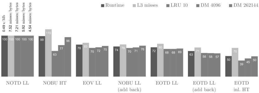
Figure 4: Main comparison diagram for performance measures across the file set, excluding adversary. Branch data structures are either linked lists (ll, where new entries are added at the front unless add back is stated), or a single hash table.

	$\text{size}\cdot$	notd	eotd	eov	eov	nobu	move down
File	$10^{-6}$	rs	rs+sl	rs	climb	climb	branch ops
chr22${}^{\text{B1}}$	34.55	29 569 178	18 927 812	318 499	33 064 133	33 669 019	35 053 371
dna${}^{\text{A1}}$	104.86	87 681 116	58 585 203	236 634	100 172 270	100 736 053	111 372 537
dblp${}^{\text{A2}}$	104.86	54 757 925	14 743 305	32 980	55 418 573	55 594 399	73 784 654
rctail96${}^{\text{B2}}$	114.71	74 993 651	20 777 946	86 190	71 863 312	72 128 546	70 211 436
jdk13c${}^{\text{B3}}$	69.73	50 659 938	6 678 647	54 174	49 300 828	49 413 385	28 044 490
sources${}^{\text{A3}}$	104.86	80 270 528	30 753 392	191 755	75 419 031	75 953 764	70 537 447
w3c2${}^{\text{B3}}$	104.20	80 056 887	12 933 438	57 108	75 773 161	75 904 742	41 111 077
english${}^{\text{A4}}$	104.86	86 528 338	43 803 204	109 151	78 451 578	78 998 269	85 577 767
etext${}^{\text{B4}}$	105.28	73 446 539	40 782 335	106 811	73 482 182	74 097 636	99 131 563
howto${}^{\text{B4}}$	39.42	28 590 381	13 523 660	89 650	27 703 460	27 944 722	32 676 237
rfc${}^{\text{B4}}$	116.42	88 716 588	32 739 584	452 280	83 618 480	84 486 767	77 334 572
pitches${}^{\text{A5}}$	55.83	47 744 716	21 303 582	279 505	42 615 067	43 081 419	46 777 918
proteins${}^{\text{A6}}$	104.86	74 912 821	39 662 469	31 075	70 942 644	71 016 405	111 979 688
sprot34${}^{\text{B7}}$	109.62	70 190 029	20 737 274	45 034	69 274 605	69 425 197	78 927 702
adversary${}^{\text{A8}}$	25.00	41 662 928	16 323	8 313 003	41 654 774	68033 898 010	12 249

Table 1: Operation counts. rs: rescan branch operations, sl: extra sibling lookup (see section 1), move down: branch operations outside of rescan. Files from the Pizza and Chili Corpus (${}^{\text{A}}$) and Lightweight Corpus (${}^{\text{B}}$). File categories are dna (${}^{\text{1}}$), xml (${}^{\text{2}}$), source code (${}^{\text{3}}$), text (${}^{\text{4}}$), midi (${}^{\text{5}}$), proteins (${}^{\text{6}}$), database (${}^{\text{7}}$), and nobu adversary (${}^{\text{8}}$).

Fig. 4 shows performance across seven implementations and five performance measures (explained in section 5.1), which we deem to be relevant for comparison. It summarizes the runtimes (also in table 2) and memory access measures by taking averages across all files except adversary, with equal weight per file. The bars are scaled to show percentages of the measures for the basic notd implementation, which is used as the benchmark. The order of the implementations when ranked by performance is fairly consistent across the different measures, with some deviation in particular for the hardware cache measure and smaller-cache models. The hardware cache measurement comes out as a relatively poor predictor of performance; by the numbers reported by Perf, the hardware cache even appears to be outperformed by our simplistic theoretical cache model.

We detect only a minor improvement of eotd ll implementations in relation to nobu ll, while inline eotd ht provides a more significant improvement. Note, however that for nobu, the ht implementation is much worse than the ll implementation, while the reverse is true for eotd. This can be attributed to the different hash table use and the particular significance of inlining, noted in section 3. The fact that eotd ht without inlining (not in the diagram) is not clearly better than nobu ht stands to confirm this. Although table 2 shows that eotd ll beats its ht counterpart for files producing a low average out-degree in ${\mathcal{ST}}$ (because of a small alphabet and/or high repetitiveness), the robustness of hashing (cf. fig 3) has the greater impact on average. We have included results to show the impact of the add to back heuristic in eotd ll, which also produced a slight improvement for nobu (not shown in diagram), as expected.

The operation counts shown in table 1 generally confirm our expectations. (Branch counts include moves down from $\topnode$ to the root, in order to match Senft and Dvořák’s corresponding counts [19].) eov yields a large rescan reduction, even for the adversary file, which makes it an attractive alternative to nobu when branching is very expensive. We found the exact choice of the $k$ parameter of eov not to be overly delicate. All values shown were obtained with $k=5$.

6 Conclusion

It is possible to significantly improve online suffix tree construction time through modifications that target reducing branch operations and cache utilization, while maintaining linear worst-case time complexity. In many applications, our representation variants should be directly applicable for runtime reduction. Interesting topics remaining to explore are how our techniques for, e.g., suffix link orientation, fit into the compromise game of time versus space in succinct representations such as compressed suffix trees, and comparison to off-line construction.

	notd	notd	nobu	nobu	nobu	eov	eov	eotd	eotd	eotd	eotd
File		ht		back	ht	ll	ht	ll	ht	back	inl. ht
chr22	11.43	16.73	8.66	9.00	13.72	9.08	14.26	8.96	14.40	8.80	8.91
dblp	29.31	35.56	22.41	21.90	30.60	23.60	32.15	20.35	26.55	17.67	16.91
dna	40.37	60.76	30.65	32.12	51.66	32.70	53.77	31.60	53.37	30.97	32.89
english	64.26	50.99	45.65	46.36	42.11	47.47	43.34	42.70	42.77	36.64	26.21
etext	64.96	50.15	47.68	46.44	42.43	50.37	44.30	45.56	43.38	39.06	27.67
howto	21.74	15.43	16.12	15.09	12.64	16.48	12.92	15.33	12.50	12.56	7.61
jdk13c	7.97	23.24	6.39	6.53	19.29	6.97	20.24	5.72	14.46	5.27	6.76
pitches	46.65	21.34	34.66	28.98	18.40	35.38	19.07	34.08	17.26	26.34	10.55
proteins	104.49	49.60	74.30	74.46	41.95	76.49	44.27	75.73	46.18	70.55	31.97
rctail96	35.67	44.76	26.72	26.54	37.44	27.61	38.35	24.59	31.32	21.18	18.35
rfc	52.58	50.81	38.78	37.22	42.96	40.55	44.14	37.18	39.99	29.45	21.82
sources	44.21	44.23	32.71	30.12	37.24	34.27	38.63	31.49	34.28	24.70	17.76
sprot34	50.19	42.65	38.40	37.92	37.37	39.82	38.50	36.71	33.66	33.24	21.24
w3c2	18.98	39.84	14.38	15.19	33.13	14.89	33.73	12.91	24.98	11.41	10.47
adversary	1.30	7.89	267.50	266.16	296.42	1.64	8.07	1.40	5.10	1.39	1.34

Table 2: Running times in seconds for the same files as table 1

References

- [1] Apostolico, A.: The myriad virtues of subword trees. In: Apostolico, A., Galil, Z. (eds.) Combinatorial Algorithms on Words, nato asi Series, vol. F 12, pp. 85–96. Springer-Verlag (1985)
- [2] Arbitman, Y., Naor, M., Segev, G.: Backyard cuckoo hashing: Constant worst-case operations with a succinct representation. In: Proc. 51st Ann. ieee Symp. Foundations of Comput. Sci. pp. 787–796 (2010)
- [3] Cánovas, R., Navarro, G.: Practical compressed suffix trees. In: Proc. 9th International Symposium on Experimental Algorithms. pp. 94–105 (2010)
- [4] Clark, D.R., Munro, J.I.: Efficient suffix trees on secondary storage. In: Proc. seventh Ann. acm–siam Symp. Discrete Algorithms. pp. 383–391 (1996)
- [5] Farach, M.: Optimal suffix tree construction with large alphabets. In: Proc. 38th Ann. ieee Symp. Foundations of Comput. Sci. pp. 137–143 (Oct 1997)
- [6] Ferragina, P.: Suffix tree construction in hierarchical memory. In: Encyclopedia of Algorithms, pp. 922–925. Springer (2008)
- [7] Ferragina, P., Navarro, G.: Pizza & chili corpus (2005), http://pizzachili.dcc.uchile.cl/
- [8] Frigo, M., Leiserson, C., Prokop, H., Ramachandran, S.: Cache-oblivious algorithms. In: Proc. 40th Ann. ieee Symp. Foundations of Comput. Sci. pp. 285–297 (1999)
- [9] Giegerich, R., Kurtz, S., Stoye, J.: Efficient implementation of lazy suffix trees. Software – Practice and Experience 33(11), 1035–1049 (2001)
- [10] Gusfield, D.: Algorithms on Strings, Trees, and Sequences. Cambridge University Press (1997)
- [11] Hagerup, T., Miltersen, P.B., Pagh, R.: Deterministic dictionaries. Journal of Algorithms 41(1), 69–85 (2001)
- [12] Kiełbasa, S.M., Wan, R., Sato, K., Horton, P., Frith, M.C.: Adaptive seeds tame genomic sequence comparison. Genome research 21(3), 487–493 (2011)
- [13] Kurtz, S.: Reducing the space requirement of suffix trees. Software – Practice and Experience 29(13), 1149–71 (1999)
- [14] Larsson, N.J.: Extended application of suffix trees to data compression. In: Proc. ieee Data Compression Conf. pp. 190–199 (Mar–Apr 1996)
- [15] Manber, U., Myers, G.: Suffix arrays: A new method for on-line string searches. siam J. Comput. 22(5), 935–948 (Oct 1993)
- [16] Manzini, G., Ferragina, P.: Lightweight corpus (2004), http://people.unipmn.it/manzini/lightweight/corpus/
- [17] McCreight, E.M.: A space-economical suffix tree construction algorithm. J. acm 23(2), 262–272 (Apr 1976)
- [18] Perf: Linux profiling with performance counters, https://perf.wiki.kernel.org/
- [19] Senft, M., Dvořák, T.: On-line suffix tree construction with reduced branching. Journal of Discrete Algorithms 12(0), 48–60 (2012)
- [20] Tian, Y., Tata, S., Hankins, R.A., Patel, J.M.: Practical methods for constructing suffix trees. The vldb Journal 14(3), 281–289 (2005)
- [21] Tsirogiannis, D., Koudas, N.: Suffix tree construction algorithms on modern hardware. In: Proc. 13th International Conference on Extending Database Technology. pp. 263–274 (2010)
- [22] Ukkonen, E.: On-line construction of suffix trees. Algorithmica 14(3), 249–260 (Sep 1995)
- [23] Weiner, P.: Linear pattern matching algorithms. In: Proc. 14th Ann. ieee Symp. Switching and Automata Theory. pp. 1–11 (1973)