On the probability distribution function of the mass surface density of molecular clouds I

The probability distribution function (PDF) of the mass surface density is an essential characteristic of the structure of molecular clouds or the interstellar medium in general. Observations of the PDF of molecular clouds indicate a composition of a broad distribution around the maximum and a decreasing tail at high mass surface densities. The first component is attributed to the random distribution of gas which is modeled using a log-normal function while the second component is attributed to condensed structures modeled using a simple power-law. The aim of this paper is to provide an analytical model of the PDF of condensed structures which can be used by observers to extract information about the condensations. The condensed structures are considered to be either spheres or cylinders with a truncated radial density profile at cloud radius $r_{\rm cl}$. The assumed profile is of the form $\rho(r)=\rho_{\rm c}/(1+(r/r_{0})^{2})^{n/2}$ for arbitrary power $n$ where $\rho_{\rm c}$ and $r_{0}$ are the central density and the inner radius, respectively. An implicit function is obtained which either truncates (sphere) or has a pole (cylinder) at maximal mass surface density. The PDF of spherical condensations and the asymptotic PDF of cylinders in the limit of infinite overdensity $\rho_{\rm c}/\rho(r_{\rm cl})$ flattens for steeper density profiles and has a power law asymptote at low and high mass surface densities and a well defined maximum. The power index of the asymptote $\Sigma^{-\gamma}$ of the logarithmic PDF ($\Sigma P(\Sigma)$) in the limit of high mass surface densities is given by $\gamma=(n+1)/(n-1)-1$ (spheres) or by $\gamma=n/(n-1)-1$ (cylinders in the limit of infinite overdensity).

1 Introduction

Observations of the structure of molecular clouds provide insights about the physical processes in the cold dense phase of the interstellar medium and will give us a better understanding how they evolve and eventually form stars. They are furthermore essential to test theoretical models of the origin of the stellar mass function (Padoan et al., 1997b; Elmegreen, 2001; Padoan & Nordlund, 2002; Hennebelle & Chabrier, G., 2008; Elmegreen, 2011; Hopkins, 2013a) and the star formation rate (Krumholz & McKee, 2005; Padoan & Nordlund, 2011; Hennebelle & Chabrier, 2011; Federrath & Klessen, 2012) which are both thought to be related to the density structure of a turbulent molecular gas.

The high resolution and sensitivity of modern telescopes allows a detailed analysis of the 1-point statistic or probability distribution function (PDF) of the mass surface density of molecular cloud gas. They are obtained using either the reddening of stars (Kainulainen et al., 2009; Froebrich & Rowles, 2010; Lombardi et al., 2010; Kainulainen & Tan, 2013; Alves et al., 2014) or more recently the infrared emission of dust grains (Hill et al., 2011, 2012; Schneider et al., 2012, 2013b, 2013a; Russeil et al., 2013).

Despite the complexity of the molecular clouds the observed PDFs of the mass surface density show very similar properties. They all are characterized by a broad peak and a tail at high mass surface densities approximately given by a power law. The PDF at low mass surface densities around the broad peak is attributed to randomly moving gas commonly referred to as ’turbulence’ while the tail is attributed to self-gravitating cloud structures. The relative amount of the two different components seems to be related to the star formation activity in the cloud as discussed by Kainulainen et al. (2009). While non-star forming clouds as the ’Coalsack’ or the ’Lupus V’ region show only a very low or no evidence of a tail the PDFs of star forming clouds as ’Taurus’ or ’Orion’ are characterized by a strong tail with no clear separation between the two components.

The observations seem to be broadly consistent with current simulations of turbulent molecular clouds. Turbulence would naturally create a wide range of densities and simulations of driven isothermal turbulence have shown that the corresponding PDF has a log-normal form (Vazquez-Semadeni, 1994; Padoan et al., 1997a; Passot & Vázquez-Semadeni, 1998), a result which has been confirmed analytically (Nordlund & Padoan, 1999). The projection of the density of those simulations has also been found to be closely log-normal in shape (Ostriker et al., 2001; Vázquez-Semadeni & García, 2001; Federrath et al., 2010; Brunt et al., 2010a). Deviations are expected for non isothermal turbulence which produces higher probabilities at low or high densities (Scalo et al., 1998; Passot & Vázquez-Semadeni, 1998; Li et al., 2003). More recent simulations of forced turbulence also show depending on the assumed forcing for the PDF of the volume density a deviation from the log-normal function with enhanced probabilities at low densities (Federrath et al., 2008; Konstandin et al., 2012; Federrath, 2013). The functional form is as shown by Federrath (2013) approximately described by a statistical function proposed by Hopkins (2013b).

Simulations of the time evolution of molecular clouds have shown that at late stage the PDF of the volume density would develop a tail-like structure at high density values (Klessen, 2000; Dib & Burkert, 2005; Vázquez-Semadeni et al., 2008). The same behavior is also seen in the PDF of the mass surface density (Ballesteros-Paredes et al., 2011; Kritsuk et al., 2011; Federrath & Klessen, 2013).

Currently, observed PDFs are analyzed using a log-normal function for the peak and a simple power law for the tail, respectively. The log-normal function allows a first estimate of the density contrast of the volume density in a turbulent medium based on the fundamental relation of the statistical properties of the mass surface density and the ones of the volume density as provided by Fischera & Dopita (2004) and also by Brunt et al. (2010b, a). The interpretation of the tail is frequently based upon a simple power law density profile $\rho(r)\propto r^{-n}$ of spheres where the PDF of the mass surface density is also a power law. In case of the logarithmic PDF ($\Sigma P(\Sigma)=P(\ln\Sigma)$) the corresponding power law would be $\Sigma^{-\gamma}$ with $\gamma=2/(n-1)$ (Kritsuk et al., 2011; Federrath & Klessen, 2013). Applying this relation the slope of the tail of the PDF of a number of star forming molecular clouds indicates a radial density profile with a power index $n\sim 2$ (Schneider et al., 2013a) as expected for collapsing clouds. A different approach has been chosen by Kainulainen & Tan (2013) who also applied a log-normal function to the tail.

However, the analytical functions show partly strong deviations to the observed curves. Most of the PDFs published by Kainulainen et al. (2009) reveal a tail at low mass surface densities below the peak which cannot be explained in terms of the simple analytical function. The tail at high mass surface densities has several features which are not expected using simple power law profiles of the radial density. Foremost, the tail is restricted to a certain range of mass surface densities. For a number of PDFs published by Kainulainen et al. (2009) the tail indicates a strong cutoff or a strong change of the slope around $A_{V}=6-10\leavevmode\nobreak\ {\rm mag}$. The interpretation of the tail is further complicated by the observational facts that condensed clouds are generally located on a certain background level and that they are restricted to small regions within the cloud complex as e.g. in case of the Rosette molecular cloud (Schneider et al., 2012). The tail is therefore not necessarily a simple power law nor directly related to the radial density profile. Furthermore, the analytical functions do not provide a physical explanation for the peak position of the PDF which occurs in case of a number of molecular clouds around $A_{V}\sim 1\leavevmode\nobreak\ {\rm mag}$.

In this and the following papers an analytical physical model of the global PDF of molecular clouds is developed which resembles the main observed features and is meant to derive basic physical parameters of star forming molecular clouds as the pressure and the density contrast in the turbulent gas. This paper focuses on the 1-point statistical properties of individual condensed structures, assumed to be spheres and cylinders.

In Sect. 2 an analytical solution of the mass surface density and the corresponding PDFs for the considered shapes is presented which is based on a truncated analytical density profile widely used in astrophysical problems. In Sect. 3 the properties of the PDFs are discussed and asymptotes for low and high mass surface densities are provided. Also studied is the location of the maximum position of the logarithmic and linear PDF. A summary is given in Sect. 4. The technical details can be found in the appendices.

2 Model of the PDF of the mass surface density of condensed structures

2.1 Radial density profiles

Let us assume for the condensed structures a simple analytical density profile given by

$$\rho(r)=\frac{\rho_{\rm c}}{(1+(r/r_{0})^{2})^{n/2}},$$ (1)

where $\rho_{\rm c}$ is the density in the cloud center and $r_{\rm 0}$ the inner radius. The density profile has a flat part in the inner region $(r\ll r_{0})$ which approaches asymptotically a power law $\rho\propto r^{-n}$ at large radii $(r\gg r_{0})$. In studies of stellar clusters this inner radius is frequently referred to as ‘core radius’ (King, 1962, 1966a, 1966b). The analytical profile is used in astrophysics for its convenience and as generalization of physical density profiles to model the stellar surface brightness of Globular clusters (e. g. Elson et al. 1987; Elson 1992) and more recently the dust emission of dense filaments (e. g. Arzoumanian et al. 2011; Malinen et al. 2012; Juvela et al. 2012).

We make another reasonable assumption that the profile is truncated at radius $r_{\rm cl}$ as expected if the clouds are cold structures embedded in warmer gas. In case of pressure equilibrium the gas pressure at the outer boundary of the condensed structure would be equal to the pressure $p_{\rm ext}$ in the surrounding medium. We refer to the inverse of the density ratio $\rho(r_{\rm cl})/\rho_{\rm c}=q$ of the density at cloud radius and cloud center as ‘overdensity’. In case of isothermal clouds this ratio is identical with the term ’overpressure’ used to characterize the gravitational state of self-gravitating structures in previous studies of pressurized clouds (Fischera & Dopita, 2008; Fischera, 2011; Fischera & Martin, 2012b, a).

Specific profiles with certain values of the power $n$ are known solutions for the physical problem of self-gravitating gaseous clouds. The profile for $n=5$ is valid for a gaseous sphere where the temperature of the gas is regulated by the adiabatic law with a ratio 1.2 of the two specific heats (Schuster, 1884; Jeans, 1916). This density profile has been applied to describe the surface brightness profiles of globular clusters and is known as Plummer-model (Plummer, 1911, 1915). The density profiles which correspond to the power indices $n=2$, $3$, and $4$ are related to profiles of isothermal self-gravitating clouds.

The profile with $n=4$ is the exact solution for a self-gravitating isothermal cylinder (Stodólkiewicz, 1963; Ostriker, 1964). The radial density profile of pressurized isothermal self-gravitating spheres, referred to as Bonnor-Ebert sphere (Ebert, 1955; Bonnor, 1956), cannot be expressed through a simple analytical formula. However, the profile for spherical clouds up to an overdensity $\sim 100$ is in excellent agreement with the analytical profile with $n=3$. The profile with $n=3$ is also identical with the well known King model without truncation (King, 1962, 1966a). The radial density profile of spheres with higher overdensity might be approximated with a profile where $n=2$. The statistical properties of isothermal clouds are analyzed in more detail in a forthcoming paper (Fischera, 2014).

2.2 Mass surface density profiles

The mass surface density profile of a truncated analytical density profile (Eq. 1) of a sphere or a cylinder seen at inclination angle $i$ where $i=0^{\circ}$ refers to a cylinder seen edge-on is given by

$$\Sigma_{n}(r)=\frac{2}{\cos^{\beta}i}\int\limits_{0}^{r_{\rm cl}\sqrt{1-(r/r_{\rm cl})^{2}}}{\rm d}l\frac{\rho_{\rm c}}{(1+(r^{2}+l^{2})/r_{\rm 0}^{2})^{n/2}}.$$ (2)

where $\beta=0$ for spheres and $\beta=1$ for cylinders. In the following it is convenient to define a parameter

$$y_{n}=(1-q^{2/n})(1-x^{2}),$$ (3)

where $x=0\leq r/r_{\rm cl}\leq 1$ is the normalized impact parameter where $r$ is the projected radius and $r_{\rm cl}$ the cloud radius. The profile of the mass surface density can then be written as

$$\Sigma_{n}(x)=\frac{2}{\cos^{\beta}i}r_{0}\rho_{c}q^{\frac{n-1}{n}}(1-y_{n})^{\frac{1-n}{2}}\int\limits_{0}^{u_{\rm max}}\frac{{\rm d}u}{(1+u^{2})^{n/2}},$$ (4)

where

$$u_{\rm max}=\sqrt{\frac{y_{n}}{1-y_{n}}}.$$ (5)

In case of isothermal self-gravitating pressurized clouds the product of inner radius and central density is proportional to $\sqrt{p_{\rm ext}}$ and is given by

$$r_{0}\rho_{c}=\sqrt{\frac{\xi_{n}p_{\rm ext}}{4\pi G}}\frac{1}{\sqrt{q}},$$ (6)

where $p_{\rm ext}$ is the external pressure, $G$ the gravitational constant and where $\xi_{2}=2$, $\xi_{3}=8.63$, and $\xi_{4}=8$ (Fischera, 2014).

It is convenient to consider the normalized mass surface density

$$X_{n}=\Sigma_{n}\cos^{\beta}i\,(2\rho_{\rm c}r_{0})^{-1}q^{-\frac{n-1}{n}},$$ (7)

which depends only on the parameter $y_{n}$. The functional dependence is shown in Fig. 1.

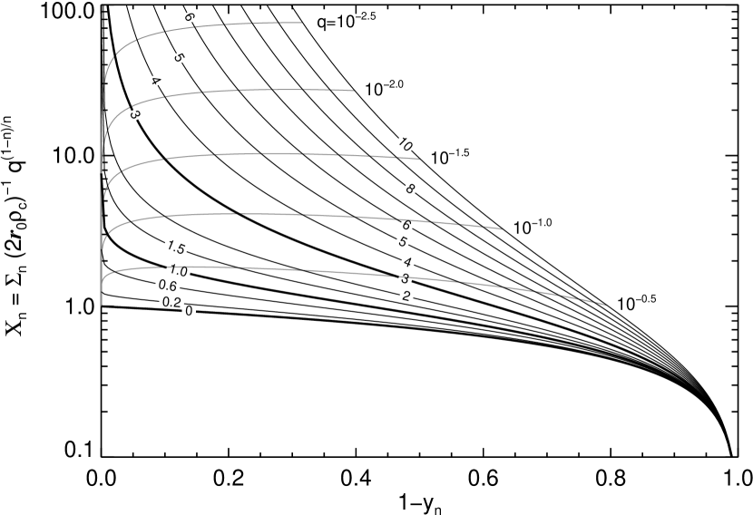
Figure 1: Normalized mass surface density $X_{n}$ as function of $1-y_{n}$ for truncated density profiles as given in Eq. 1 for various power indices $n$ ranging from 0 to 10. The thicker lines correspond to $n=0$, 1, and 3. For a fixed pressure ratio $q$ the mass surface densities for a given power index $n$ vary from the central value at $1-y_{n}=q^{2/n}$ to zero at the edge of the cloud where $1-y_{n}=1$. The central values of the normalized mass surface density for various pressure ratios $q$ are shown as thin gray lines.

Profiles of the normalized mass surface density for a number of different assumptions for the power index $n$ of a truncated density profile are shown in Fig. 2. The method used to derive the profiles is described in Sects. A.1 and A.2. The profiles for $n=1$, 2, 3, and 4 are simple analytical functions given in App. A.3. At an overdensity of 10 the inner part of the profiles of cylinders and spheres closely resembles a Gaussian approximation with a width as given in Sect. A.4.

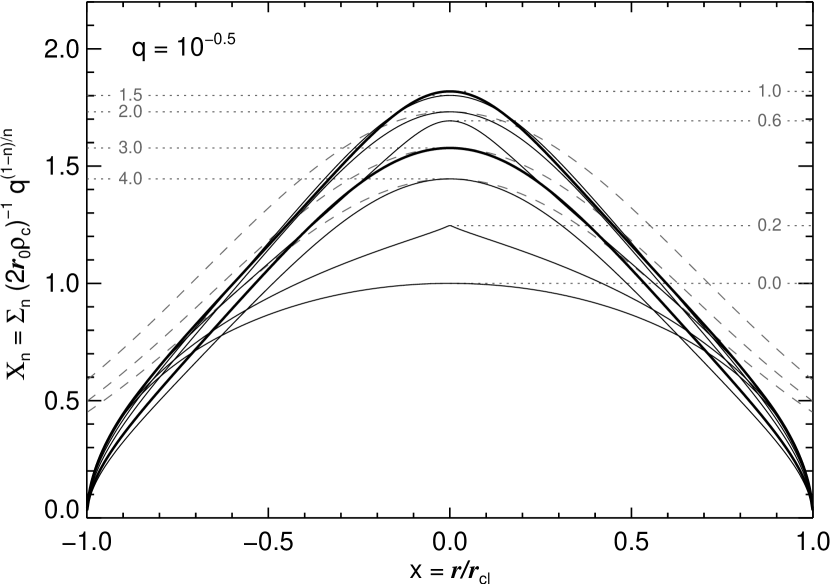
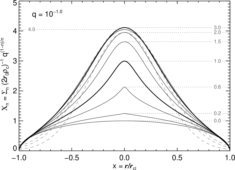
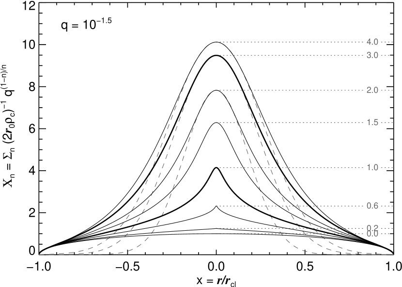
Figure 2: Profiles of the normalized mass surface density $X_{n}$ of a truncated density profile as given in Eq. 1 for three assumptions of the pressure ratio $q=p_{\rm ext}/p_{\rm c}$. The maxima or the curves are labeled with the corresponding power index $n$. The profiles for $n=1$ and $n=3$ are enhanced with a thicker line. The dashed lines are Gaussian approximations (Eq. 46) where the variance is obtained using Eq. 45. The profile for $n=0$ need to be considered as an asymptote.

2.3 PDF of the mass surface density

The PDF of the mass surface density can be given as an implicit function of $y_{n}$. In the limit $y_{n}\rightarrow 1$ and $y_{n}\rightarrow 0$ also explicit expressions of the asymptotic behavior of the PDF can be given and are discussed.

The PDF for the mass surface density is given by

$$P(\Sigma_{n}(x))=\frac{{\rm d}P}{{\rm d}\Sigma_{n}}=-P(r)\left(\frac{{\rm d}\Sigma_{n}}{{\rm d}r}\right)^{-1},$$ (8)

where $P(r)$ is the probability to measure a mass surface density at impact radius $r$. For a sphere this is given by $P(r)=2\pi r/(\pi r_{\rm sph}^{2})=2x/r_{\rm sph}$ and for a cylinder $P(r)=1/r_{\rm cyl}$. It is convenient to consider the PDF of the normalized mass surface density as defined in Eq. 7 which is given by

$$P(X_{n})=P(\Sigma_{n})\frac{1}{\cos^{\beta}i}(2r_{0}\rho_{\rm c})q^{\frac{n-1}{n}}.$$ (9)

with $\beta=0$ for spheres and $\beta=1$ for cylinders.

By taking the derivative of Eq. 4 it is straightforward to show that

$$\frac{{\rm d}X_{n}}{{\rm d}r}=-(1-q^{2/n})\frac{x}{r_{\rm cl}}\frac{1+(n-1)\sqrt{y_{n}}X_{n}}{\sqrt{y_{n}}(1-y_{n})}.$$ (10)

For spheres we obtain the implicit function

$$P_{\rm sph}(X_{n})=\frac{2}{1-q^{2/n}}\frac{\sqrt{y_{n}}(1-y_{n})}{1+(n-1)\sqrt{y_{n}}X_{n}(y_{n})}.$$ (11)

As we see the normalized PDF $(1-q^{2/n})P_{\rm sph}(X_{n})$ is an implicit function of the parameter $y_{n}$ alone. The corresponding PDF for cylinders is

$$P_{\rm cyl}(X_{n})=\frac{1}{2x}P_{\rm sph}(X_{n}),$$ (12)

where the normalized impact parameter can be expressed through

$$x=\sqrt{\frac{1-y_{n}-q^{2/n}}{1-q^{2/n}}}.$$ (13)

The PDF has a pole at the maximum mass surface density ($x=0$) or where $y_{n}=1-q^{2/n}$ (Fig. 3).

Because of the pole for cylinders we have therefore not a generalized form of the PDF that depends only on the parameter $y_{n}$. However, to obtain an expression which allows a similar discussion in the following section for spheres and cylinders we can consider the asymptotic PDF for infinitely high overdensity. In the limit $1-y_{n}\gg q^{2/n}$ the impact parameter behaves as

$$x\approx\sqrt{1-y_{n}}.$$ (14)

We consider therefore the following asymptotic PDF

$$P^{(a)}_{\rm cyl}(X_{n})=\frac{1}{1-q^{2/n}}\frac{\sqrt{y_{n}}\sqrt{1-y_{n}}}{1+(n-1)\sqrt{y_{n}}X_{n}(y_{n})}.$$ (15)

As shown in App. B the asymptotic PDF provides for all $q$ the correct asymptote in the limit of small mass surface densities and the correct asymptotic behavior at large mass surface densities for $q\rightarrow 0$.

3 Characteristics of the PDF

The PDFs of spheres and the asymptotic PDFs of cylinders with a truncated analytical density profile for various different assumptions for the power $n$ and the pressure ratio $q$ are shown in Fig. 4. They are truncated at the highest mass surface density.

The exact asymptotes for high and low mass surface densities also shown in the figure are derived in Sect. B. The maximum position is discussed in more detail in Sect. C.

The curves have a functional form that depends only on the power $n$ of the radial density profile. They are truncated at the central mass surface density.

3.1 Asymptotes at high and low mass surface densities

At low mass surface densities the PDF approaches asymptotically a power law $P(\Sigma)\propto\Sigma$. The asymptotic behavior at high mass surface densities depends on the steepness of the radial density profile. For $n>1$ the PDF approaches asymptotically a power law given by

$$P_{\rm sph}(X_{n})\propto X_{n}^{-\frac{n+1}{n-1}},\quad P_{\rm cyl}^{(a)}(X_{n})\propto X_{n}^{-\frac{n}{n-1}}.$$ (16)

As can be seen in the figure the asymptote is a better representation of the PDF at high mass surface densities for steeper density profiles. In the limit of large power $n$ the PDF at high mass surface densities becomes $P(X_{n})\propto X_{n}^{-1}$ as expected for a source with a Gaussian density profile (Sect. B.3.1). For $n=1$ the PDF at high mass surface density is an exponential function

$$P_{\rm sph}(X_{n})\propto e^{-2X_{1}},\quad P_{\rm cyl}^{(a)}(X_{n})\propto e^{-X_{1}}.$$ (17)

For clouds with $n<1$ the PDF is limited to a maximum mass surface density given by $X_{n}=1/(1-n)$. In the neighborhood of this maximum value the PDF varies strongly with mass surface density. In the limit of $n=0$ the PDF becomes identical to the PDF of a homogeneous sphere or cylinder.

The power law asymptote at high mass surface densities may be used to infer the power $n$ of the radial density profile. For spheres a power law $P_{\rm sph}\propto\Sigma^{-\alpha}$ would indicate a power index $n=(\alpha+1)/(\alpha-1)$ of the radial density profile as can be derived for simple power law density profiles (Kritsuk et al., 2011; Federrath & Klessen, 2013). As shown in Fig. 3 the asymptotic behavior at large mass surface densities in case of cylinders is only established for sufficiently high overdensities. For example, a profile with $n=4$ which is consistent with the density profile of self-gravitating isothermal cylinders the PDF for overdensities as high as 100 has no apparent power law at high mass surface densities. For cylinders with high overpressure the PDF at the pole is approximately given by $P_{\rm cyl}(X_{n})\propto X_{n}^{-\frac{n}{n-1}}/\sqrt{1-(X_{n}/X_{n}(0))^{2/(n-1)}}$ A power law is only established for the range $[X_{n}]_{\rm max}\ll X_{n}\ll X_{n}(0)$ where $[X_{n}]_{\rm max}$ is the mass surface density at the PDF maximum (Sect. 3.2).

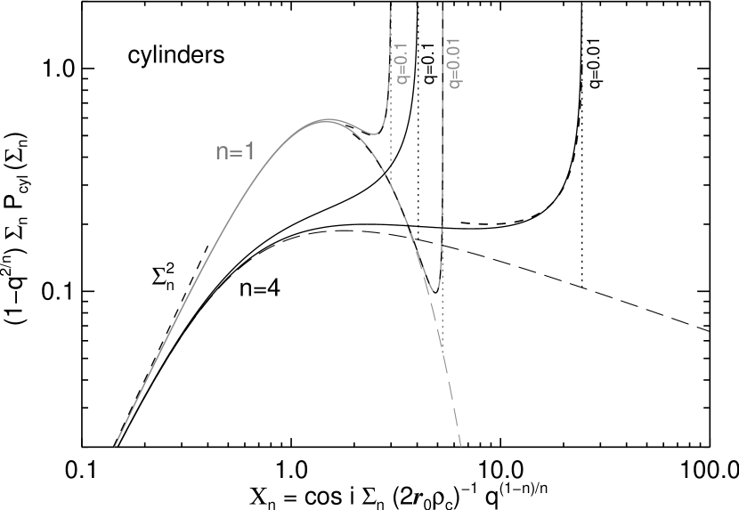
Figure 3: PDF of the normalized mass surface density $X_{n}$ of cylindrical clouds having a density distribution with $n=1$ (gray lines) and $n=4$ (black lines). The clouds have an overdensity ($1/q$) of either 10 or 100. The long dashed curves show the asymptote for infinite high overdensity. The dotted lines mark the asymptotic value at the poles. The short dashed lines give the asymptotic values in the limit of high and low values of $X_{n}$.

Figure 4: PDF of the normalized mass surface density $X_{n}$ in case of spheres (top figure) and the asymptotic PDF in case of cylinders (bottom figure) with a truncated radial density profile given by Eq. 1 for various assumptions of the power $n$. The thin lines show at which mass surface density $X_{n}$ at given density ratio $q=\rho(r_{\rm cl})/\rho_{\rm c}$ the PDF corresponding to a certain power $n$ truncates (for spheres) or has a pole (for cylinders). The lines are labeled with $\log_{10}q$. The dashed lines show the asymptotic behavior at large and small $X_{n}$.

3.2 The maxima of the asymptotic PDF

As we see in Fig. 4 the PDF of spheres and the asymptotic PDF of cylinders with the analytical density profile have well defined maxima at $[X_{n}]_{\rm max}$ which depend only on the power $n$. This allows a simple interpretation of the observed mass surface density at the peak position in terms of the normalization factor $2r_{0}\rho_{\rm c}q^{(n-1)/n}$ for given $n$ using the definition Eq. 7. In case of isothermal clouds the maximum position can be used to infer the pressure in the ambient medium.

Table 1: Maxima positions of the linear and logarithmic PDF

		sphere $P_{\rm sph}(X_{n})$		cylinder $P^{(a)}_{\rm cyl}(X_{n})$
n	PDF	$[y_{n}]_{\rm max}$	$[X_{n}]_{\rm max}$	$[y_{n}]_{\rm max}$	$[X_{n}]_{\rm max}$
1	$P(X_{n})$	$\frac{1}{3}$	$\ln\frac{\sqrt{3}+1}{\sqrt{2}}$	$\frac{1}{2}$	$\ln[1+\sqrt{2}]$
2	$P(X_{n})$	0.2110	0.5373	0.2723	0.7277
3	$P(X_{n})$	$\frac{2-\sqrt{3}}{\sqrt{3}}$	$\frac{\sqrt{2\sqrt{3}-3}}{2\sqrt{3}-2}$	$\frac{\sqrt{33}-5}{4}$	$2\frac{\sqrt{\sqrt{33}-5}}{9-\sqrt{33}}$
4	$P(X_{n})$	0.1222	0.4162	0.1413	0.4609
1	$X_{n}P(X_{n})$	0.5861	1.0096	0.8069	1.4633
2	$X_{n}P(X_{n})$	0.4780	1.0566	0.6547	1.6041
3	$X_{n}P(X_{n})$	$\sqrt{2}-1$	$\frac{\sqrt{2\sqrt{2}-2}}{2\sqrt{2}-2}$	$\frac{\sqrt{17}-3}{2}$	$\frac{\sqrt{2\sqrt{17}-6}}{5-\sqrt{17}}$
4	$X_{n}P(X_{n})$	0.3700	1.1367	0.4970	1.7974

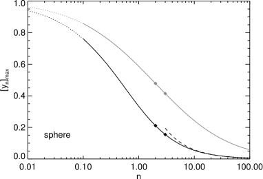
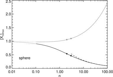
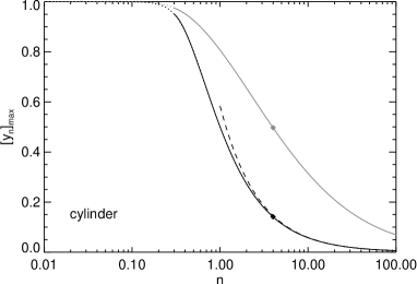
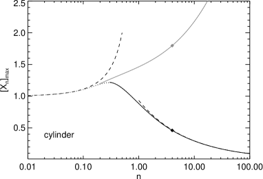
Figure 5: Maxima position of the PDF of the parameter $y_{n}$ and the normalized mass surface density $X_{n}$ for spheres (top) and cylinders (bottom) as function of the power $n$ (dotted curves). Black lines correspond to the linear PDF and the gray lines to logarithmic PDF. The solid curves are polynomial fits to the accurate position values. The values for isothermal self-gravitating spheres ($n=2$ and $n=3$) and cylinders ($n=4$) are shown as small diamonds. The asymptotic behavior of $[X_{n}]_{\rm max}=1/(1-n)$ for $n\rightarrow 0$ for cylinders is shown as dashed line. Asymptotes described in Sect. C.1.1 are shown as dashed lines.

Related to the maximum position is a parameter $[y_{n}]_{\rm max}$. The functional dependence of the maximum position $[y_{n}]_{\rm max}$ and $[X_{n}]_{\rm max}$ of the linear and logarithmic asymptotic PDF on the power $n$ is shown in Fig. 5. The curves are derived by solving the conditional equations given in App. C. Selected values are given in Tab. 1.

As shown in Sect. B.3.2, in the limit $n\rightarrow 0$ the PDFs become the ones of homogeneous spheres and cylinders where the maximum value is related to the central mass surface density. In this limit we have therefore $[y_{n}]_{\rm max}\rightarrow 1$ and $[X_{n}]_{\rm max}=1$. In case of cylinders the normalized mass surface density at PDF maximum in the limit of flat density profiles is approximately given by $[X_{n}]_{\rm max}=1/(1-n)$.

The parameter $[y_{n}]_{\rm max}$ provides for given power $n$ an estimate of the corresponding impact parameter as function of the pressure ratio $q$ based on Eq. 13. Below a minimum overpressure $(1-[y_{n}]_{\rm max})^{-n/2}$ the maximum coincides with the central mass surface density. At higher overpressures the impact parameter moves outwards and reaches asymptotically a maximum value $x=\sqrt{1-[y_{n}]_{\rm max}}$. If we consider for example the logarithmic PDF of a sphere with $n=3$ the minimum overdensity with $x=0$ is

$$q^{-1}=\left(1-\left[\sqrt{2}-1\right]\right)^{-3/2}\approx 2.23,$$ (18)

where the parameter $[y_{n}]_{\rm max}$ is taken from Tab. 1. In the limit $q\rightarrow 0$ the impact parameter at the PDF maximum becomes

$$x=\sqrt{1-\left[\sqrt{2}-1\right]}\approx 0.765.$$ (19)

As the maximum position $[y_{n}]_{\rm max}$ decreases with $n$ the impact parameter related to the PDF maximum is larger for steeper density profiles and reaches $x=1$ for $n\rightarrow\infty$. In case of the logarithmic PDF the mass surface density related to the PDF maximum is larger in respect to the linear PDF and corresponds to a smaller impact parameter.

The dependence of the maxima of the linear PDF in the limit $n\rightarrow\infty$ can be described by simple power laws as shown in App. C.1.1. The asymptotes for $[y_{n}]_{\rm max}$ and $[X_{n}]_{\rm max}$ provide as shown in Fig. 5 good results for spheres above $n\approx 3$ and for cylinders above $n\approx 1$.

Table 2: Coefficients of the polynomial approximation of the maximum position of the asymptotic PDF

	$a_{1}$	$a_{2}$	$a_{3}$	$a_{4}$	$a_{5}$	$a_{6}$	$n_{\rm min}$	$n_{\rm max}$
Spheres, linear values
$[y_{n}]_{\rm max}$	-1.099	-0.5883	-0.1071	0.004447	0.002598	-0.0003259	0.1	100.0
$[X_{n}]_{\rm max}$	-0.4181	-0.2544	-0.05889	0.0008424	0.001723	-0.0001919	0.1	100.0
Spheres, log values
$[y_{n}]_{\rm max}$	-0.5338	-0.2590	-0.04989	-0.002858	0.0004857	—	0.1	100.0
$[X_{n}]_{\rm max}$	0.008622	0.04882	0.02353	0.003190	-0.0003657	—	0.1	100.0
Cylinders, linear values
$[y_{n}]_{\rm max}$	-0.6920	-0.8029	-0.1382	0.05612	-0.01153	0.0009113	0.3	100.0
$[X_{n}]_{\rm max}$	-0.1243	-0.4190	-0.07131	0.03418	-0.007760	0.0006513	0.3	100.0
Cylinders, log values
$[y_{n}]_{\rm max}$	-0.2146	-0.2506	-0.07477	0.002226	0.0001414	—	0.3	100.0
$[X_{n}]_{\rm max}$	0.3806	0.1235	0.01110	0.006071	-0.0007028	—	0.2	100.0

The ratio

$$\frac{[\Sigma_{n}]_{\rm cut}}{[\Sigma_{n}]_{\rm max}}=\frac{[X_{n}]_{\rm cut}}{[X_{n}]_{\rm max}}$$ (20)

between the central mass surface density $[X_{n}]_{\rm cut}$ and the mass surface at the PDF maximum can be used to infer the pressure ratio $q$ for given power $n$. As an example we consider a critical stable sphere which radial density profile is close to the analytical profile with $n=3$. The critical stable sphere has a density ratio of $q\approx 1/14.04$ Applying Eq. 37 we find that the corresponding central mass surface density is given by

$$[X_{3}]_{\rm cut}=q_{\rm crit}^{-\frac{2}{3}}\sqrt{1-q_{\rm crit}^{2/3}}\approx 5.296.$$ (21)

For critical stable spheres the ratio between the cutoff and the maximum of the logarithmic PDF is therefore given by

$$\frac{[X_{3}]_{\rm cut}}{[X_{3}]_{\rm max}}=q_{\rm crit}^{-\frac{2}{3}}\sqrt{1-q_{\rm crit}^{2/3}}\frac{2\sqrt{2}-2}{\sqrt{2\sqrt{2}-2}}\approx 4.821,$$ (22)

where the maximum position is taken from Tab. 1.

The functional dependence of the maximum position on the power $n$ can over a large range be well fitted by a polynomial function

$$[y_{n}]_{\rm max} = \sum_{i=1}^{N_{\rm max}}a_{i}(\ln n)^{i},$$ (23)

$$\ [X_{n}]_{\rm max} = \sum_{i=1}^{N_{\rm max}}a_{i}(\ln n)^{i},$$ (24)

where $N_{\rm max}=6$ for spheres and $N_{\rm max}=5$ for cylinders. The coefficients are listed in Tab. 2.

4 Summary and conclusion

The study summarizes a series of properties of the PDF of the mass surface density of spherical and cylindrical structures having an analytical radial density profile $\rho=\rho_{\rm c}/(1+(r/r_{0})^{2})^{n/2}$ where $\rho_{c}$ is the central density and $r_{0}$ the inner radius. The profiles are assumed to be truncated at a cloud radius $r_{\rm cl}$ as expected for cold structures embedded in a considerably warmer medium. The results are therefore applicable to individual condensed structures in star forming molecular clouds.

The PDF for given geometry is determined by the power $n$, the density ratio $q=\rho(r_{\rm cl})/\rho_{\rm c}$, the product $\rho_{\rm c}r_{0}$, and, in case of a cylinder, the inclination angle $i$. It is convenient to describe the properties of the PDF in terms of the unit free mass surface density defined by

$$X_{n}=\Sigma_{n}\frac{\cos^{\beta}i}{2\rho_{\rm c}r_{0}}q^{-\frac{n-1}{n}},$$ (25)

where $\beta=0$ for spheres and $\beta=1$ for cylinders. The properties are:

1. For given geometry and power index $n$ the normalized PDF $(1-q^{2/n})P(X_{n})$ is a unique curve expressed through a simple implicit function of the parameter $y_{n}=(1-q^{2/n})(1-x^{2})$ where $x=r/r_{\rm cl}$ is the normalized impact parameter.

2. At the central mass surface density $X_{n}(0)$ the PDF of spheres has a sharp cut-off while the PDF of cylinders has a pole.

3. At high overdensities the PDF has a well defined maximum at fixed $[X_{n}]_{\rm max}$.

4. At mass surface densities which are small relative to the maximum position the asymptotic PDF approaches asymptotically a power law $P(X_{\rm n})\propto X_{n}$.

5. In the limit of high overdensities the PDFs approach for $n>1$ at mass surface densities above the peak asymptotically power laws. They are given by $P(X_{n})\propto X_{n}^{-\frac{n+1}{n-1}}$ in case of spheres and, with the exception of the pole, by $P(X_{n})\propto X^{-\frac{n}{n-1}}$ in case of cylinders. For given overdensity the asymptote is a better approximation for steeper density profiles (larger $n$).

6. For $n<1$ the PDF has a strong cutoff and is limited to a maximum mass surface density $X_{n}\leq 1/(1-n)$.

The slope of the PDF at high mass surface densities can also be obtained assuming a simple power law profile for spherical clouds (e.g. Kritsuk et al. 2011; Federrath & Klessen 2013). But it should be considered that this profile only is an asymptotic behavior in the limit of high overdensities and seems more appropriate for collapsing clouds while most condensations might not be in such a state. As shown in the paper in general the shape of the PDF is not a power law. Further, the profile would produce a nonphysical high probability at low mass surface densities.

The derived properties are related to background subtracted structures within molecular clouds. They are therefore not directly applicable to measurements of the global PDF of molecular clouds which is a statistical mean of different properties not only of the condensed structures but the surrounding medium as well. For instance the tail at high mass surface densities seen in the PDF of star forming molecular clouds may have different physical explanations. It also need to be considered that the functional form of the PDF is affected by an additional background. In case of filaments the situation is furthermore complicated through a possible variation of the inclination angle. Those problems are addressed in a following paper (Fischera, 2014) based on isothermal self-gravitating pressurized spheres and cylinders.

Appendix A Solution for the mass surface density profile

A.1 Case $n\geq 1$

In case $n>1$ the integral can be expressed through the incomplete and complete beta function

$$\int\limits_{0}^{u_{\rm max}}\frac{{\rm d}u}{(1+u^{2})^{\frac{n}{2}}} = \frac{1}{2}{\rm B}\left(\frac{n}{2}-\frac{1}{2},\frac{1}{2}\right)$$ (26)

$$\times\bigg{\{}1-I_{1-y_{n}}\left(\frac{n}{2}-\frac{1}{2},\frac{1}{2}\right)\bigg{\}},$$

with the condition $a,b>0$ where the normalized incomplete beta function is given by

$$I_{\xi}(a,b)=\frac{1}{B(a,b)}\int_{0}^{\xi}{\rm d}t\,t^{a-1}(1-t)^{b-1}.$$ (27)

The beta function is equal to

$${\rm B}(a,b)=\frac{\Gamma(a)\Gamma(b)}{\Gamma(a+b)},$$ (28)

where $\Gamma(x)$ is the $\Gamma$-function given by

$$\Gamma(x)=\int_{0}^{\infty}{\rm d}t\,t^{x-1}e^{-t}.$$ (29)

In Sect. D the asymptotic behavior of $I_{\xi}(a,b)$ with $a=(n-1)/2$ and $b=0.5$ is discussed. In general the asymptotic behavior is better for higher powers of $a$.

The mass surface density for given external pressure and overdensity through the cloud center for $n>1$ is

$$\Sigma_{n}(0)=\frac{r_{0}\rho_{c}}{\cos^{\beta}i}\,{\rm B}\left(\frac{n-1}{2},\frac{1}{2}\right)\left\{1-I_{q^{2/n}}\left(\frac{n-1}{2},\frac{1}{2}\right)\right\}.$$ (30)

In the limit of high overdensity ($q\rightarrow 0$) the central mass surface density becomes the asymptotic value

$$\Sigma_{n}(0)\approx\frac{r_{0}\rho_{c}}{\cos^{\beta}i}\frac{\Gamma(\frac{n-1}{2})\Gamma(\frac{1}{2})}{\Gamma(\frac{n}{2})}.$$ (31)

A.2 Case $n<1$

To estimate the profile for $n<1$ we can transform the integral to

$$\int\limits_{0}^{u_{\rm max}}\frac{{\rm d}u}{(1+u^{2})^{\frac{n}{2}}} = \frac{1}{n-1}\Bigg{\{}n\int\limits_{0}^{u_{\rm max}}\frac{{\rm d}u}{(1+u^{2})^{\frac{n}{2}+1}}$$ (32)

$$-\frac{u_{\rm max}}{(1+u_{\rm max}^{2})^{\frac{n}{2}}}\Bigg{\}}.$$

The integral can then be calculated using the complete and incomplete beta function as in Eq. 26. The mass surface density profile becomes

$$\Sigma_{n}(x) = \frac{2}{\cos^{\beta}i}r_{0}\rho_{c}q^{\frac{n-1}{n}}\frac{1}{1-n}\Bigg{\{}\sqrt{y_{n}}$$ (33)

$$-n(1-y_{n})^{\frac{1-n}{2}}\int\limits_{0}^{u_{\rm max}}\frac{{\rm d}u}{(1+u^{2})^{\frac{n}{2}+1}}\Bigg{\}}.$$

In the limit of high overdensity the central mass surface density approaches asymptotically a maximum value given by

$$\Sigma_{n}(0)=\frac{2}{\cos^{\beta}i}r_{0}\rho_{c}q^{\frac{n-1}{n}}\frac{1}{1-n}.$$ (34)

A.3 Analytical profiles of the mass surface densities

The mass surface density profiles of the truncated analytical density profile for any natural number $n=1,2,...$ can be expressed through simple analytical functions. For $n=1$, $2$, $3$, and $4$ the profiles are for example given by

$$\Sigma_{1}(x) = \frac{2}{\cos^{\beta}i}(r_{0}\rho_{c})\ln\left[\frac{1+\sqrt{y_{1}}}{\sqrt{1-y_{1}}}\right],$$ (35)

$$\Sigma_{2}(x) = \frac{2}{\cos^{\beta}i}\rho_{c}r_{0}q^{\frac{1}{2}}\frac{1}{\sqrt{1-y_{2}}}\tan^{-1}\sqrt{\frac{y_{2}}{1-y_{2}}},$$ (36)

$$\Sigma_{3}(x) = \frac{2}{\cos^{\beta}i}\rho_{c}r_{0}q^{\frac{2}{3}}\frac{1}{1-y_{3}}\sqrt{y_{3}},$$ (37)

$$\Sigma_{4}(x) = \frac{2}{\cos^{\beta}i}\rho_{c}r_{0}q^{\frac{3}{4}}\frac{1}{(1-y_{4})^{3/2}}\frac{1}{2}$$ (38)

$$\times\Bigg{\{}\sqrt{y_{4}}\sqrt{1-y_{4}}+\tan^{-1}\sqrt{\frac{y_{4}}{1-y_{4}}}\Bigg{\}},$$

where $y_{n}=(1-x^{2})(1-q^{2/n})$. The profiles of higher orders can be derived by applying successively the integral transform Eq. 32.

The profile $n=4$ applies for isothermal self-gravitating pressurized cylinders. For cylinders exist a maximum mass line density given by $[M/l]_{\rm max}=2K/G$ where $G$ is the gravitational constant. $K$ is a constant given by $K=kT/(\mu m_{\rm H})$ where $T$ is the effective temperature, $k$ the Boltzmann constant, $\mu$ the mean molecular weight and $m_{\rm H}$ is the atomic mass of hydrogen. If we replace the pressure ratio with $q=(1-f)^{2}$ where $f=(M/l)/[M/l]_{\rm max}\leq 1$ is the normalized mass line density we obtain the expression given in the work of Fischera & Martin (2012a). The profile for $n=3$ closely describes the profile of Bonnor-Ebert spheres with overdensities less than $\sim 100$ (Fischera, 2014).

A.4 Gaussian approximation ($n\rightarrow\infty$)

Under certain circumstances the inner region of the profile can be approximated by a Gaussian function as will be shown in the following where the width is related to physical parameters as the overdensity $q^{-1}$ and the inner radius $r_{0}$.

The density profile can in general be expressed through

$$\rho(x)=\rho_{\rm c}e^{-\frac{n}{2}\ln\left[1+(xr_{\rm cl}/r_{0})^{2}\right]},$$ (39)

where

$$\frac{r^{2}_{\rm cl}}{r^{2}_{0}}=q^{-\frac{2}{n}}\left(1-q^{\frac{2}{n}}\right).$$ (40)

Where $(xr_{\rm cl}/r_{0})^{2}\ll 1$ we can linearize the logarithm using $\ln[1+(xr_{\rm cl}/r_{0})^{2}]\approx(xr_{\rm cl}/r_{0})^{2}$ and we obtain a Gaussian density profile

$$\rho(x)=\rho_{\rm c}e^{-\frac{1}{2}\left(\frac{x}{\sigma_{\rho}}\right)^{2}},$$ (41)

where the variance is given by

$$\sigma_{\rho}^{2}=\frac{1}{n}\frac{r^{2}_{0}}{r^{2}_{\rm cl}}=\frac{1}{n}\frac{q^{\frac{2}{n}}}{1-q^{\frac{2}{n}}}.$$ (42)

The approximation improves with power $n$. In case of a pressure ratio $q$ the density profile becomes approximately a Gaussian function for all impact parameters if $n\gg-2\ln q/\ln 2$ or $q^{\frac{2}{n}}\gg\frac{1}{2}$. For large $n$ the variance becomes

$$\sigma_{\rho}^{2}\rightarrow-\frac{1}{2\ln q},$$ (43)

which decreases slowly with overdensity.

In a similar approach we can derive the asymptotic profile of the mass surface density. Considering the same condition for $n$ as above we obtain for example for

$$(1-y_{n})^{\frac{1-n}{2}}=q^{\frac{1-n}{n}}e^{-\frac{1}{2}\left(\frac{x}{\sigma_{\Sigma}}\right)^{2}},$$ (44)

also a Gaussian form where the variance of the mass surface density is given by

$$\sigma^{2}_{\Sigma}=\frac{1}{{n-1}}\frac{r_{0}^{2}}{r_{\rm cl}^{2}}=\frac{1}{n-1}\frac{q^{\frac{2}{n}}}{1-q^{\frac{2}{n}}},$$ (45)

where $\sigma_{\Sigma}\approx\sigma_{\rho}=\sigma$ for large $n$.

The central region ($x\ll r_{0}/r_{\rm cl}$) of the profile is therefore approximately given by a Gaussian function

$$\Sigma_{n}\approx\rho_{\rm c}r_{0}e^{-\frac{1}{2}\left(\frac{x}{\sigma}\right)^{2}}{\rm B}\left(\frac{n-1}{2},\frac{1}{2}\right)\left(1-I_{q^{\frac{2}{n}}}\left(\frac{n-1}{2},\frac{1}{2}\right)\right).$$ (46)

The approximation provides the exact central mass surface density.

We want to consider the case of high overdensity and large power $n$ so that the contribution of the incomplete beta function in the central region of the cloud becomes negligible (see Sect. D). In the limit of large $n$ the beta function becomes

$$\frac{\Gamma\left(\frac{n-1}{2}\right)\Gamma\left(\frac{1}{2}\right)}{\Gamma\left(\frac{n}{2}\right)}\rightarrow\sqrt{\frac{2\pi}{n}}.$$ (47)

Replacing $n$ through the variance of the density profile we obtain for the asymptotic profile for given overdensity

$$\Sigma_{\infty}(x)\rightarrow\rho_{\rm c}\sqrt{2\pi}\sigma r_{\rm cl}\,e^{-\frac{1}{2}\left(\frac{x}{\sigma}\right)^{2}}=\Sigma_{\infty}(0)e^{-\frac{1}{2}\left(\frac{x}{\sigma}\right)^{2}}.$$ (48)

Appendix B Asymptotes of the PDF

B.1 Asymptotes in the limit $y_{n}\rightarrow 0$ (low $X_{n}$)

In the limit of large impact parameters ($x\rightarrow 1$) it follows that $y_{n}\rightarrow 0$ and consequently $u_{\rm max}\approx\sqrt{y_{n}}\ll 1$. The integrand in Eq. 4 is approximately a constant so that the unit-free mass surface density becomes

$$X_{n}\approx\sqrt{y_{n}}.$$ (49)

From Eq. 11 we find directly the corresponding asymptotic behavior for spheres which is given by

$$P_{\rm sph}(X_{n})\approx\frac{2}{1-q^{2/n}}X_{n}.$$ (50)

For cylinders we find from Eq. 15

$$P_{\rm cyl}(X_{n})\approx P_{\rm cyl}^{(a)}(X_{n})\approx\frac{1}{1-q^{2/n}}X_{n}.$$ (51)

For $q^{2/n}\rightarrow 0$ we obtain the asymptote of the probability function of homogeneous spheres or cylinders.

B.2 Asymptotes in the limit $y_{n}\rightarrow 1$ (high $X_{n}$)

B.2.1 Asymptotes for $n>1$

In the limit of low impact parameter ($x\rightarrow 0$) and high overdensity ($q\ll 1$) we have $y_{n}\rightarrow 1-q^{2/n}\sim 1$. The normalized mass surface density is then approximately given by

$$X_{n}\sim(1-y_{n})^{\frac{1-n}{2}}\zeta_{n}\gg 1,$$ (52)

where $\zeta_{n}=0.5\,{\rm B}((n-1)/2,1/2)$. We can use this relation to replace $1-y_{n}$ to obtain an expression of the PDF as function of the mass surface density.

For the PDF of spheres we find that at high mass surface densities the PDF approaches asymptotically a power law given by

$$P_{\rm sph}(X_{n})\sim\frac{1}{n-1}\frac{2}{1-q^{2/n}}X_{n}^{-\frac{n+1}{n-1}}\zeta_{n}^{\frac{2}{n-1}}.$$ (53)

For the asymptotic PDF of cylinders we find

$$P^{(a)}_{\rm cyl}(X_{n})\sim\frac{1}{n-1}\frac{1}{1-q^{2/n}}X_{n}^{-\frac{n}{n-1}}\zeta_{n}^{\frac{1}{n-1}}.$$ (54)

Replacing $1-y_{n}$ in the Eq. 12 with the above expression for the mass surface density provides the asymptotic behavior of the PDF of cylinders at the pole given by

$$P_{\rm cyl}(X_{n})\sim\frac{1}{n-1}\frac{1}{\sqrt{1-q^{2/n}}}\frac{X_{n}^{-\frac{n}{n-1}}\zeta^{\frac{1}{n-1}}}{\sqrt{1-(X_{n}/X_{n}(0))^{\frac{2}{n-1}}}},$$ (55)

where $X_{n}(0)=q^{\frac{1-n}{n}}\zeta_{n}$ is the central mass surface density. A power law is only established for cylinders with sufficiently high overpressure so that $(X_{n}/X_{n}(0))^{2/(n-1)}\ll 1$.

B.2.2 Asymptotes for $n=1$

In the limit of large $y_{1}$ the mass surface density behaves as

$$X_{1}\sim\ln\frac{2}{\sqrt{1-y_{1}}}.$$ (56)

Replacing

$$1-y_{1}\approx 4\,e^{-2X_{1}}$$ (57)

in Eq. 11 and in Eq. 15 provides the asymptotes

$$P_{\rm sph}(X_{1})\approx\frac{2}{1-q^{2}}(1-y_{n})\sim\frac{8}{1-q^{2}}e^{-2X_{1}}$$ (58)

for and

$$P^{(a)}_{\rm cyl}(X_{1})\approx\frac{1}{1-q^{2}}\sqrt{1-y_{n}}\sim\frac{2}{1-q^{2}}e^{-X_{1}}.$$ (59)

For the special case $n=1$ the PDF at high mass surface densities is therefore approximately described by a simple exponential function. The asymptotic behavior of the PDF for a cylinder including the region at the pole is

$$P_{\rm cyl}(X_{1})\approx\frac{2}{\sqrt{1-q^{2}}}\frac{e^{-X_{1}}}{\sqrt{1-e^{-2(X_{1}(0)-X_{1})}}},$$ (60)

where $X_{1}(0)=\ln(2q^{-1})$.

B.2.3 Asymptotes for $n<1$

As pointed out in Sect. A.2 for $n<1$ the mass surface density has a maximum possible value. In the limit $y_{n}\rightarrow 1$ we have

$$X_{n}\approx\frac{1}{1-n}\sqrt{y_{n}}\leq\frac{1}{1-n}.$$ (61)

As can be shown we have $P_{\rm sph}(X_{n})\rightarrow 0$ and $P_{\rm cyl}^{(a)}(X_{n})\rightarrow 0$ for $X_{n}\rightarrow 1/(1-n)$.

B.3 Asymptote of the PDF for high/low $n$

B.3.1 Asymptote in the limit $n\rightarrow\infty$

As we have seen in the previous section in the limit of high $n$ the power law slope at high mass surface densities approaches asymptotically $\alpha=1$. The corresponding PDF can be directly obtained from Eq. 53. Replacing $n-1$ by the standard deviation of the Gaussian approximation we get for spheres with high overdensity in the limit of $n\rightarrow\infty$

$$P_{\rm sph}(X_{n})\sim 2\sigma^{2}X_{n}^{-1}.$$ (62)

The same result is obtained from Eq. 48 by deriving the corresponding derivative and using Eq. 8. For the asymptotic PDF of cylinders Eq. 54

$$P^{(a)}_{\rm cyl}(X_{n})\sim\sigma^{2}X_{n}^{-1}.$$ (63)

B.3.2 Asymptote in the limit $n\rightarrow 0$

In the limit $n\rightarrow 0$ it follows from Eq. 33 for the mass surface density

$$X_{n}\rightarrow\frac{1}{1-n}\sqrt{y_{n}}.$$ (64)

In case of spheres the PDF of the mass surface density becomes

$$P_{\rm sph}(X_{n})\approx\frac{2}{1-q^{2/n}}\sqrt{y_{n}}\rightarrow 2\sqrt{1-x^{2}},$$ (65)

which is the PDF of homogeneous spheres. Likewise, we find for the asymptotic PDF of cylindrical clouds in the limit $n\rightarrow 0$ that

$$P^{(a)}_{\rm cyl}(X_{n})\approx P_{\rm cyl}(X_{n})\rightarrow\frac{\sqrt{1-x^{2}}}{x},$$ (66)

which is the PDF of a homogeneous cylinder.

Appendix C Condition for PDF maxima

The maxima position were derived for both linear and logarithmic PDFs of spheres and cylinders. For cylinders the asymptotic PDF as defined in Eq. 15 was considered.

C.1 For linear values ($P(\Sigma_{n})$)

The condition for maxima of the linear PDF is given by

$$\frac{{\rm d}P}{{\rm d}y_{n}}(X_{n})=0.$$ (67)

This leads to

$$X_{n}y_{n}^{\frac{3}{2}}(n^{2}-1)+y_{n}(n+2)-1=0$$ (68)

in case spheres and to

$$X_{n}y_{n}^{\frac{3}{2}}n(n-1)+y_{n}(n+1)-1=0$$ (69)

for cylinders. For $n=1$ and $n=3$ the maxima are simple analytical expressions listed in Tab. 1.

C.1.1 Approximation for $n\gg 1$

In the limit $n\gg 1$ the condition for maxima of the linear PDF is equal for spheres and cylinders and is given by

$$X_{n}y_{n}^{\frac{3}{2}}n^{2}+y_{n}n-1=0.$$ (70)

As $y_{n}\rightarrow 0$ for $n\rightarrow\infty$ it follows from Eq. 85 and Eq. 47 that the mass surface density behaves approximately as

$$X_{n}\sim e^{\frac{n}{2}y_{n}}\frac{1}{2}\sqrt{\frac{2\pi}{n}}P(\chi^{2},1),$$ (71)

where $P(\chi^{2},1)$ is the PDF of the $\chi^{2}$-distribution and where

$$\chi^{2}\rightarrow ny_{n}.$$ (72)

In the limit of $n\gg 1$ the condition for maxima becomes a function of $ny_{n}=C$ where $C$ is a constant. Solving

$$e^{C/2}\sqrt{\frac{\pi}{2}}P(C,1)C^{\frac{3}{2}}+C-1=0$$ (73)

provides $C\approx 0.58404$. The maxima position is therefore approximately given by

$$[y_{n}]_{\rm max} = C/n,$$ (74)

$${[X_{n}]}_{\rm max} = e^{C/2}\sqrt{\frac{\pi}{2n}}P(C,1).$$ (75)

C.2 For logarithmic values ($\Sigma_{n}P(\Sigma_{n})$)

The maxima of the PDF of logarithm values are given by the condition

$$\frac{{\rm d}}{{\rm d}y_{n}}[X_{n}P(X_{n})]=0.$$ (76)

This leads to

$$2X_{n}^{2}y_{n}(n-1)-X_{n}\left((n-1)\sqrt{y_{n}}+\frac{1-3y_{n}}{\sqrt{y_{n}}}\right)=1$$ (77)

in case of spheres and to

$$X_{n}^{2}y_{n}(n-1)-X_{n}\left((n-1)\sqrt{y_{n}}+\frac{1-2y_{n}}{\sqrt{y_{n}}}\right)=1$$ (78)

in case of cylinders. For $n=3$ the maxima positions are again simple analytical expressions given in Tab. 1.

Appendix D Asymptotic behavior of the incomplete beta function

To derive the asymptotic behavior of the incomplete beta function in Eq. 4 for the mass surface density in the limit $n\gg 1$ we consider the approximation (Eq. 26.5.20, of Abramowitz & Stegun (1972))

$$I_{\xi}(a,b) \sim 1-P(\chi^{2},\nu),$$ (79)

$$= \left(2^{\frac{\nu}{2}}\Gamma\left(\frac{\nu}{2}\right)\right)^{-1}\int\limits_{\chi^{2}}^{\infty}{\rm d}t\,t^{\frac{\nu}{2}-1}\,e^{-\frac{t}{2}},$$

where $P(\chi^{2},\nu)$ is the $\chi^{2}$ distribution function of $\nu$ events where

$$\chi^{2} = (a+b-1)(1-\xi)(3-\xi)-(1-\xi)(b-1),$$ (80)

$$\nu = 2b.$$ (81)

In our case we have $a=(n-1)/2$ and $b=1/2$. The incomplete beta function is then approximately given by

$$I_{1-y_{n}}\left(\frac{n-1}{2},\frac{1}{2}\right)\sim\frac{1}{\sqrt{2\pi}}\int\limits_{\chi^{2}}^{\infty}{\rm d}t\,t^{-\frac{1}{2}}e^{-\frac{t}{2}},$$ (82)

where

$$\chi^{2}=\left(\frac{n-2}{2}\right)y_{n}(2+y_{n})+y_{n}\frac{1}{2}.$$ (83)

For given power $n$ the approximation improves with increasing $\xi$.

In the limit $y_{n}\rightarrow 0$ we can use the replacement

$$(1-y_{n})^{\frac{1-n}{2}}\sim e^{\frac{n-1}{2}y_{n}},$$ (84)

so that the mass surface density becomes

$$\Sigma_{n}\sim 2r_{0}\rho_{\rm c}q^{\frac{n-1}{n}}e^{-\frac{1-n}{2}y_{n}}\frac{1}{2}{\rm B}\left(\frac{n-1}{2},\frac{1}{2}\right)P(\chi^{2},1).$$ (85)

In the limit $n\rightarrow\infty$ we have

$$\chi^{2}\approx ny_{n}\rightarrow-2\,(1-x^{2})\,\ln q,$$ (86)

so that the beta function becomes independent of $n$.

D.1 Incomplete beta function for $b=1/2$

The power law approximation of the PDF at large mass surface densities for $n>1$ as presented in Sect. B are valid for negligible contribution of the incomplete beta function to the mass surface density. We have seen in Fig. 4 that the power law is only a good representation for large mass surface densities and that the approximation of the PDF improves for larger $n$.

Fig. 6 shows the value of the incomplete beta function as given in Eq. 4 for different assumptions for the powers $n$ and the density ratio $q$. As we see the value of the incomplete beta function for given $q$ decreases for larger $n$. In the limit $n\rightarrow\infty$ for given $q$ we obtain the asymptotic value of the incomplete beta function given in the previous section. In the limit $n\rightarrow 1$ we have

$$I_{1-y_{n}}\left(\frac{n-1}{2},\frac{1}{2}\right)\rightarrow 1.$$ (87)

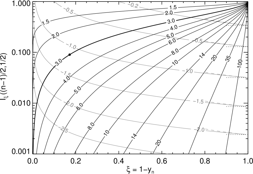
Figure 6: Incomplete beta function $I_{\xi}(a,b)$ (black contours) for $a=(n-1)/2$ and $b=1/2$ as function of $\xi=1-y_{n}$. The lines are labeled with the corresponding power $n$. The line for a power $n=3$ is emphasized through a thick line. The gray lines correspond to $\xi=q^{2/n}$ for fixed density ratio $q$ and varying power $n$. The lines are labeled with $\log_{10}q$. The gray dashed lines are obtained using the approximation of the incomplete beta function (Eq. 82). The asymptotic value of the incomplete beta function for given $q$ in the limit $n\rightarrow\infty$ is indicated through dotted lines. The filled circle corresponds to a power $n=3$ and an overdensity $q_{\rm crit}^{-1}=14.04$ of a critical stable sphere.

References

- Abramowitz & Stegun (1972) Abramowitz, M. & Stegun, I. A., eds. 1972, Handbook of Mathematical Functions (National Bureau of Standards)
- Alves et al. (2014) Alves, J., Lombardi, M., & Lada, C. 2014, A&A, in press, DOI: 10.1051/0004-6361/201322159
- Arzoumanian et al. (2011) Arzoumanian, D., André, P., Didelon, P., et al. 2011, A&A, 529, L6
- Ballesteros-Paredes et al. (2011) Ballesteros-Paredes, J., Vázquez-Semadeni, E., Gazol, A., et al. 2011, MNRAS, 416, 1436
- Bonnor (1956) Bonnor, W. B. 1956, MNRAS, 116, 351
- Brunt et al. (2010a) Brunt, C. M., Federrath, C., & Price, D. J. 2010a, MNRAS, 405, L56
- Brunt et al. (2010b) Brunt, C. M., Federrath, C., & Price, D. J. 2010b, MNRAS, 403, 1507
- Dib & Burkert (2005) Dib, S. & Burkert, A. 2005, ApJ, 630, 238
- Ebert (1955) Ebert, R. 1955, Zeitschrift fur Astrophysik, 37, 217
- Elmegreen (2001) Elmegreen, B. G. 2001, in Astronomical Society of the Pacific Conference Series, Vol. 243, From Darkness to Light: Origin and Evolution of Young Stellar Clusters, ed. T. Montmerle & P. André, 255
- Elmegreen (2011) Elmegreen, B. G. 2011, ApJ, 731, 61
- Elson (1992) Elson, R. A. W. 1992, MNRAS, 256, 515
- Elson et al. (1987) Elson, R. A. W., Fall, S. M., & Freeman, K. C. 1987, ApJ, 323, 54
- Federrath (2013) Federrath, C. 2013, MNRAS, 436, 1245
- Federrath & Klessen (2012) Federrath, C. & Klessen, R. S. 2012, ApJ, 761, 156
- Federrath & Klessen (2013) Federrath, C. & Klessen, R. S. 2013, ApJ, 763, 51
- Federrath et al. (2008) Federrath, C., Klessen, R. S., & Schmidt, W. 2008, ApJ, 688, L79
- Federrath et al. (2010) Federrath, C., Roman-Duval, J., Klessen, R. S., Schmidt, W., & Mac Low, M.-M. 2010, A&A, 512, A81
- Fischera (2011) Fischera, J. 2011, A&A, 526, A33+
- Fischera (2014) Fischera, J. 2014, A&A, submitted
- Fischera & Dopita (2004) Fischera, J. & Dopita, M. 2004, ApJ, 611, 911
- Fischera & Dopita (2008) Fischera, J. & Dopita, M. 2008, ApJS, 176, 164
- Fischera & Martin (2012a) Fischera, J. & Martin, P. G. 2012a, A&A, 547, A86
- Fischera & Martin (2012b) Fischera, J. & Martin, P. G. 2012b, A&A, 542, A77
- Froebrich & Rowles (2010) Froebrich, D. & Rowles, J. 2010, MNRAS, 406, 1350
- Hennebelle & Chabrier (2011) Hennebelle, P. & Chabrier, G. 2011, ApJ, 743, L29
- Hennebelle & Chabrier, G. (2008) Hennebelle, P. & Chabrier, G. 2008, ApJ, 684, 395
- Hill et al. (2011) Hill, T., Motte, F., Didelon, P., et al. 2011, A&A, 533, A94
- Hill et al. (2012) Hill, T., Motte, F., Didelon, P., et al. 2012, A&A, 542, A114
- Hopkins (2013a) Hopkins, P. F. 2013a, MNRAS, 430, 1653
- Hopkins (2013b) Hopkins, P. F. 2013b, MNRAS, 430, 1880
- Jeans (1916) Jeans, J. H. 1916, MNRAS, 76, 567
- Juvela et al. (2012) Juvela, M., Malinen, J., & Lunttila, T. 2012, A&A, 544, A141
- Kainulainen et al. (2009) Kainulainen, J., Beuther, H., Henning, T., & Plume, R. 2009, A&A, 508, L35
- Kainulainen & Tan (2013) Kainulainen, J. & Tan, J. C. 2013, A&A, 549, A53
- King (1962) King, I. 1962, AJ, 67, 471
- King (1966a) King, I. R. 1966a, AJ, 71, 64
- King (1966b) King, I. R. 1966b, AJ, 71, 276
- Klessen (2000) Klessen, R. S. 2000, ApJ, 535, 869
- Konstandin et al. (2012) Konstandin, L., Girichidis, P., Federrath, C., & Klessen, R. S. 2012, ApJ, 761, 149
- Kritsuk et al. (2011) Kritsuk, A. G., Norman, M. L., & Wagner, R. 2011, ApJ, 727, L20
- Krumholz & McKee (2005) Krumholz, M. R. & McKee, C. F. 2005, ApJ, 630, 250
- Li et al. (2003) Li, Y., Klessen, R. S., & Mac Low, M.-M. 2003, ApJ, 592, 975
- Lombardi et al. (2010) Lombardi, M., Lada, C. J., & Alves, J. 2010, A&A, 512, A67
- Malinen et al. (2012) Malinen, J., Juvela, M., Rawlings, M. G., et al. 2012, A&A, 544, A50
- Nordlund & Padoan (1999) Nordlund, Å. P. & Padoan, P. 1999, in Insterstellar Turbulence, ed. J. Franco & A. Carramiñana (Cambridge University Press), 218
- Ostriker et al. (2001) Ostriker, E. C., Stone, J. M., & Gammie, C. F. 2001, ApJ, 546, 980
- Ostriker (1964) Ostriker, J. 1964, ApJ, 140, 1056
- Padoan et al. (1997a) Padoan, P., Jones, B. J. T., & Nordlund, A. P. 1997a, ApJ, 474, 730
- Padoan & Nordlund (2002) Padoan, P. & Nordlund, Å. 2002, ApJ, 576, 870
- Padoan & Nordlund (2011) Padoan, P. & Nordlund, Å. 2011, ApJ, 730, 40
- Padoan et al. (1997b) Padoan, P., Nordlund, A., & Jones, B. J. T. 1997b, MNRAS, 288, 145
- Passot & Vázquez-Semadeni (1998) Passot, T. & Vázquez-Semadeni, E. 1998, Phys. Rev. E, 58, 4501
- Plummer (1911) Plummer, H. C. 1911, MNRAS, 71, 460
- Plummer (1915) Plummer, H. C. 1915, MNRAS, 76, 107
- Russeil et al. (2013) Russeil, D., Schneider, N., Anderson, L. D., et al. 2013, A&A, 554, A42
- Scalo et al. (1998) Scalo, J., Vazquez-Semadeni, E., Chappell, D., & Passot, T. 1998, ApJ, 504, 835
- Schneider et al. (2013a) Schneider, N., André, P., Könyves, V., et al. 2013a, ApJ, 766, L17
- Schneider et al. (2012) Schneider, N., Csengeri, T., Hennemann, M., et al. 2012, A&A, 540, L11
- Schneider et al. (2013b) Schneider, N., Csengeri, T., Hennemann, M., et al. 2013b, A&A, 551, C1
- Schuster (1884) Schuster, A. 1884, Brit. Ass. Rep., 53rd Meeting (1883), 428
- Stodólkiewicz (1963) Stodólkiewicz, J. S. 1963, Acta Astronomica, 13, 30
- Vazquez-Semadeni (1994) Vazquez-Semadeni, E. 1994, ApJ, 423, 681
- Vázquez-Semadeni & García (2001) Vázquez-Semadeni, E. & García, N. 2001, ApJ, 557, 727
- Vázquez-Semadeni et al. (2008) Vázquez-Semadeni, E., González, R. F., Ballesteros-Paredes, J., Gazol, A., & Kim, J. 2008, MNRAS, 390, 769