Generalization of the Schwarz-Christoffel mapping to multiply connected polygonal domains

Abstract

A generalization of the Schwarz-Christoffel mapping to multiply connected polygonal domains is obtained by making a combined use of two preimage domains, namely, a rectilinear slit domain and a bounded circular domain. The conformal mapping from the circular domain to the polygonal region is written as an indefinite integral whose integrand consists of a product of powers of the Schottky-Klein prime functions, which is the same irrespective of the preimage slit domain, and a prefactor function that depends on the choice of the rectilinear slit domain. A detailed derivation of the mapping formula is given for the case where the preimage slit domain is the upper half-plane with radial slits. Representation formulae for other canonical slit domains are also obtained but they are more cumbersome in that the prefactor function contains arbitrary parameters in the interior of the circular domain.

I Introduction

The Schwarz-Christoffel mapping to polygonal domains is an important result in the theory of complex-valued functions and one that finds numerous applications in applied mathematics, physics, and engineering Driscoll . The applicability of Schwarz-Christoffel formula is nonetheless limited by the fact that it pertains only to simply connected polygonal domains. Therefore, there has long been considerable interest in extending the Schwarz-Christoffel transformation to multiply connected polygonal domains.

Recently, explicit formulae for generalized Schwarz-Christoffel mappings from a circular domain to both bounded and unbounded multiply connected polygonal regions have been obtained using two equivalent approaches. Using reflection arguments, DeLillo and collaborators DeLillo2004 ; DeLillo2006 derived infinite product formulae for the generalized Schwarz-Christoffel mappings, whereas Crowdy BoundedMCSC ; UnboundedMCSC used a function-theoretical approach to obtain a mapping formula in terms of the Schottky-Klein prime function associated with the circular domain. (The equivalence of the two methods was established in DeLillo2006 .) It is important to point out that both these formulations entail an implicit choice of a multiply connected rectilinear slit domain in an auxiliary preimage plane, whereby each rectilinear boundary segment of this preimage domain is mapped to a polygonal boundary (see below). The introduction of a preimage domain with rectilinear boundaries makes it possible to write down an explicit expression for the derivative of the desired conformal mapping, which can then be integrated to yield a generalised Schwarz-Christoffel formula. It is thus clear that different choices of rectilinear slit domains in the auxiliary plane will result in different formulae for the generalised Schwarz-Christoffel mapping. Therefore, a derivation of alternative representation formulae is of some interest.

In this paper a general formalism to construct conformal mappings of multiply connected polygonal domains is presented. The method applies to both bounded and unbounded polygonal domains but emphasis will be given to the bounded case as formulated in §II. A key ingredient in the approach described herein is the introduction of a multiply connected rectilinear slit domain in an auxiliary $\lambda$-plane, such that each rectilinear boundary in the $\lambda$-plane is mapped to a polygonal boundary in the $z$-plane. It is advantageous to have rectilinear boundaries in the preimage domain because the derivative of the respective conformal mapping has constant argument on each of domain’s boundaries. To derive an expression for the mapping derivative, it is expedient to introduce a slit map from a bounded multiply connected circular domain in an auxiliary $\zeta$-plane to the rectilinear slit domain in the $\lambda$-plane. Using the properties of the Schottky-Klein prime function associated with the circular domain, as summarized in §III and §IV, it is then possible to obtain an explicit expression for the derivative of the mapping from the circular domain to the polygonal region. The desired conformal mapping is then written in final form as an indefinite integral whose integrand consists of i) a product of powers of the Schottky-Klein prime functions and ii) a prefactor function, $S(\zeta)$, that depends on the choice of the rectilinear slit domain in the $\lambda$-plane.

A detailed derivation of the prefactor $S(\zeta)$ is given in §V for the case where the rectilinear slit domain consists of the upper half-plane cut along radial segments. This preimage domain turns out to be the most convenient one not only in that it naturally extends to multiply connected domains the usual treatment of simply connected polygonal regions but most importantly because it yields a simpler formula for the generalized Schwarz-Christoffel mapping. As further illustration of the method presented here, the corresponding formulae for two other canonical slit domains (including the case considered by Crowdy BoundedMCSC ) are derived in §VI. These alternative representations have, however, the inconvenience of containing certain arbitrary parameters in the interior of the circular domain. For completeness, the case of unbounded polygonal domains is briefly discussed in §VII, after which our main results and conclusions are summarized in §VIII.

II Mathematical formulation

II.1 Bounded polygonal regions

Let us consider a target region $D_{z}$ in the $z$-plane that is a bounded $(M+1)$-connected polygonal domain. The outer boundary polygon is denoted by $P_{0}$ and the $M$ inner polygons by $P_{j}$, $j=1,...,M$; see figure 1(b). Let the vertices at polygon $P_{j}$, $j=0,1,...,M$, be denoted by $z_{k}^{(j)}$, $k=1,...,n_{j}$, and let $\pi\alpha_{k}^{(j)}\in[0,2\pi]$ be the interior angles at the respective vertices. Following the notation of Driscoll & Trefethen Driscoll , we write

$$\pi\alpha_{k}^{(j)}=\pi(\beta_{k}^{(j)}+1),\qquad k=1,...,n_{j},$$ (1)

where $\pi\beta_{k}^{(j)}$ represents the turning angle at vertex $z_{k}^{(j)}$, so that the parameters $\beta_{k}^{(j)}$ must satisfy the following relations:

$$\sum_{k=1}^{n_{0}}\beta_{k}^{(0)}=-2,\qquad\sum_{k=1}^{n_{j}}\beta_{k}^{(j)}=2,\quad j=1,...,M.$$ (2)

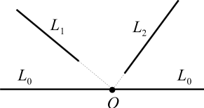
(a) $\lambda$-plane

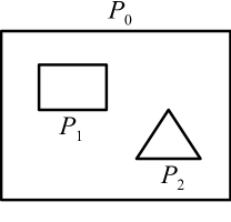
(b) $z$-plane

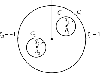
(c) $\zeta$-plane

Figure 1: (a) Radial slit domain in the upper half-$\lambda$-plane; (b) bounded polygonal domain in the $z$-plane; and (c) circular domain in the $\zeta$-plane.

II.2 Radial slit domains in the upper half-plane

Let us now consider a domain $D_{\lambda}$ in a subsidiary $\lambda$-plane consisting of the upper half-plane with $M$ slits pointing towards the origin. Denote by $L_{0}$ the real axis in the $\lambda$-plane and by $L_{j}$, $j=1,...,M$, the $M$ radial slits; see figure 1(a). We seek a conformal mapping $z(\lambda)$ from the radial slit domain $D_{\lambda}$ in the upper half-$\lambda$-plane to the polygonal domain $D_{z}$ in the $z$-plane, where the real $\lambda$-axis is mapped to the outer polygon $P_{0}$ and each radial slit $L_{j}$ is mapped to an inner polygon $P_{j}$.

If we denote by $\lambda_{k}^{(j)}$ the preimages in the $\lambda$-plane of the vertices $z_{k}^{(j)}$ on polygon $P_{j}$, $j=0,1,...,M$, then $z(\lambda)$ must have a branch point at $\lambda=\lambda_{k}^{(j)}$ such that

$$\frac{dz}{d\lambda}\approx\textrm{constant}\cdot(\lambda-\lambda_{k}^{(j)})^{\beta_{k}^{(j)}}\quad\mbox{for}\quad\lambda\to\lambda_{k}^{(j)}.$$ (3)

Furthermore, the derivative $dz/d\lambda$ must have constant arguments on each boundary segment in the $\lambda$-plane, that is,

$$\arg\left[\frac{dz}{d\lambda}\right]=\textrm{const.}\quad\mbox{for}\quad\lambda\in L_{j},\ j=0,1,...,M.$$ (4)

This follows from the fact that both $\arg[d\lambda]$ and $\arg[dz]$ are constant on the respective boundaries in the $\lambda$- and $z$-planes. In the case of simply connected polygonal regions, conditions (3) and (4) can be easily satisfied by writing $dz/d\lambda$ as a product of monomials of the type $(\lambda-\lambda_{k}^{(j)})^{\beta_{k}^{(j)}}$, leading to the well-known Schwarz-Christoffel formula Fokas . But for multiply connected domains condition (4) represents a major obstacle in deriving an explicit formula for $dz/d\lambda$, for no longer is it obvious how to construct a function that has constant argument on the multiple rectilinear boundaries of the domain $D_{\lambda}$. This obstacle can nonetheless be overcome by introducing a conformal mapping, $\lambda(\zeta)$, from a circular domain $D_{\zeta}$ in an auxiliary $\zeta$-plane to the slit domain $D_{\lambda}$. This allows us to write an explicit expression for the derivative $dz/d\lambda$ in terms of the $\zeta$ variable, as will be seen in §V.

II.3 Bounded circular domains

Let $D_{\zeta}$ be a circular domain in the $\zeta$-plane consisting of the unit disc with $M$ smaller nonoverlapping disks excised from it. Label the unit circle by $C_{0}$ and the $M$ inner circular boundaries by $C_{1},...,C_{M}$, and denote the centre and radius of the circle $C_{j}$ by $\delta_{j}$ and $q_{j}$, respectively. For convenience, we introduce the notation $\delta_{0}=0$ and $q_{0}=1$ for the unit circle. A schematic of $D_{\zeta}$ is shown in figure 1(c).

Now let $\lambda(\zeta)$ be a conformal mapping from the circular domain $D_{\zeta}$ to the domain $D_{\lambda}$ defined above, where the unit circle, is mapped to the real axis in the $\lambda$-plane and the interior circles $C_{j}$ map to the slits $L_{j}$, $j=1,...,M$. Furthermore, let the point $\zeta=1$ map to the origin in the $\lambda$-plane and the point $\zeta=-1$ map to infinity; see figures 1(a) and 1(c). In an abuse of notation, we shall write $z(\zeta)\equiv z(\lambda(\zeta))$ for the associated conformal mapping from $D_{\zeta}$ to the polygonal region $D_{z}$, where the unit circle $C_{0}$ maps to the outer polygonal boundary $P_{0}$ and the interior circles $C_{j}$ map to the inner polygons $P_{j}$; see figures 1(b) and 1(c). If we denote by $a_{k}^{(j)}$ the preimages in the $\zeta$-plane of the vertices $z_{k}^{(j)}$ on polygon $P_{j}$, then condition (3) can be recast as

$${z_{\lambda}}(\zeta)\approx\textrm{constant}\cdot(\zeta-a_{k}^{(j)})^{\beta_{k}^{(j)}}\quad\mbox{for}\quad\zeta\to a_{k}^{(j)},$$ (5)

where ${z_{\lambda}}(\zeta)$ denotes the derivative $dz/d\lambda$ expressed in terms of the $\zeta$-variable. Similarly, the requirement (4) becomes

$$\arg\left[{z_{\lambda}}(\zeta)\right]=\textrm{const.}\quad\mbox{for}\quad\zeta\in C_{j},\ j=0,1,...,M.$$ (6)

As first noticed by Crowdy BoundedMCSC , albeit in a somewhat different and less general formulation, it is possible to write an explicit expression for $z_{\lambda}(\zeta)$ that satisfies conditions (5) and (6) by exploiting the properties of the Schottky-Klein prime function associated with the circular domain $D_{\zeta}$. Once an expression for $z_{\lambda}(\zeta)$ is obtained, a corresponding expression for $z_{\zeta}(\zeta)$ follows from the chain rule which can then be integrated yielding the desired conformal mapping $z(\zeta)$, as will be shown in §V. Prior to this, however, a brief overview of the Schottky-Klein prime function is in order.

III Schottky groups and the Schottky-Klein prime function

Consider the bounded circular domain $D_{\zeta}$ defined above; see figure 1(c). Introduce the following Möbius maps:

$$\theta_{j}(\zeta)=\delta_{j}+\frac{q_{j}^{2}\zeta}{1-\bar{\delta}_{j}\zeta},\quad j=0,1,...M,$$ (7)

where a bar denotes complex conjugation. For $\zeta\in C_{j}$, it is easy to establish the following relations:

$${\zeta}={\theta_{j}}(1/\bar{\zeta})\qquad\Longleftrightarrow\qquad\bar{\zeta}=\bar{\theta}_{j}(1/\zeta),$$ (8)

where in the second identity we introduced the conjugate function $\bar{\theta}(\zeta)=\overline{\theta(\bar{\zeta})}$ .

Now let $C^{\prime}_{j}$, $j=1,...,M$, denote the reflection of the circle $C_{j}$ in the unit circle $C_{0}$. One can readily verify that every $\theta_{j}(\zeta)$ maps the interior of the circle $C_{j}^{\prime}$ onto the exterior of the circle $C_{j}$. Thus, the set $\Theta$ consisting of all compositions of the maps $\theta_{j}(\zeta)$, $j=1,...,M$, and their inverses defines a classical Schottky group Baker . The region in the complex plane exterior to all of the circles $C_{j}$ and $C_{j}^{\prime}$ is called the fundamental region, $F$, of the Scotkky group $\Theta$. Given a Scotkky group $\Theta$, we can associate a Schottky-Klein prime function, denoted by $\omega(\zeta,\alpha)$, for any two distinct points $\zeta$ and $\alpha$ in the fundamental region $F$.

The Schottky-Klein prime function has the following infinite product representation Baker :

$$\omega(\zeta,\alpha)=(\zeta-\alpha)\prod_{\theta\in\Theta^{\prime\prime}}\frac{(\zeta-\theta(\alpha))(\alpha-\theta(\zeta))}{(\zeta-\theta(\zeta))(\alpha-\theta(\alpha))},$$ (9)

where the subset $\Theta^{\prime\prime}\subset\Theta$ consists of all compositions of the maps $\theta_{j}(\zeta)$ and $\theta^{-1}_{j}(\zeta)$, excluding the identity and taking only an element or its inverse (but not both). For example, if $\theta_{1}(\theta^{-1}_{2}(\zeta))$ is included in the set $\Theta^{\prime\prime}$, then $\theta_{2}(\theta^{-1}_{1}(\zeta))$ must be excluded.

Let us now recall some useful functional identities involving the Schottky-Klein prime function. Firstly, note that by definition the Schottky-Klein prime function is antisymmetric in its two arguments:

$$\omega(\zeta,\gamma)=-\omega(\gamma,\zeta).$$ (10)

Secondly, for the Schottky-Klein prime function associated with the circular domain $D_{\zeta}$ the following functional relation

$$\bar{\omega}\left(1/\zeta,1/\gamma\right)=-\frac{1}{\zeta\gamma}\omega(\zeta,\gamma)$$ (11)

holds KRtheory . A third important relation of the Schottky-Klein prime function is as follows. Let $\zeta_{1}$, $\zeta_{2}$, $\gamma_{1}$, and $\gamma_{2}$ be four points in $F$, then we have

$$\frac{\omega(\theta_{j}(\zeta_{1}),\gamma_{1})}{\omega(\theta_{j}(\zeta_{2}),\gamma_{2})}=\frac{\beta_{j}(\gamma_{1},\gamma_{2})}{\beta_{j}(\zeta_{1},\zeta_{2})}\left(\frac{1-\bar{\delta}_{j}\zeta_{2}}{1-\bar{\delta}_{j}\zeta_{1}}\right)\frac{\omega(\zeta_{1},\gamma_{1})}{\omega(\zeta_{2},\gamma_{2})},$$ (12)

where

$$\beta_{j}(\zeta,\gamma)=\exp\left[2\pi\mathrm{i}(v_{j}(\zeta)-v_{j}(\gamma))\right],\quad j=1,...,M.$$ (13)

Equation (12) follows from a related expression given in ch. 12 of Baker Baker for the ratio ${\omega(\theta_{j}(\zeta),\gamma)}/{\omega(\zeta,\gamma)}$; see also related discussion in the monograph by Hejhal Hejhal . Here the functions $\{v_{j}(\zeta)~{}|~{}j=1,...,M\}$ are the $M$ integrals of the first kind of the Riemann surface associated with the domain $D_{\zeta}$. These are analytic but not single-valued functions everywhere in $F$. (They can be made single-valued by inserting cuts connecting each pair of circles $C_{j}$ and $C_{j}^{\prime}$; see Baker Baker .) Each function $v_{j}(\zeta)$ has constant imaginary part on the circles $C_{1},...,C_{M}$, and zero imaginary part on the unit circle $C_{0}$, that is,

$${\rm Im}[v_{j}(\zeta)]=Q_{jl}\qquad\mbox{for}\qquad\zeta\in C_{l},\ l=0,1,...,M,$$ (14)

where $Q_{jl}$ is a real constant, with $Q_{j0}=0$ CM2006 .

As particular cases of (12) we have

$$\frac{\omega(\theta_{j}(\zeta),\gamma_{1})}{\omega(\theta_{j}(\zeta),\gamma_{2})}=\beta_{j}(\gamma_{1},\gamma_{2})\frac{\omega(\zeta,\gamma_{1})}{\omega(\zeta,\gamma_{2})},$$ (15)

$$\frac{\omega(\theta_{j}(\zeta_{1}),\gamma)}{\omega(\theta_{j}(\zeta_{2}),\gamma)}=\frac{1}{\beta_{j}(\zeta_{1},\zeta_{2})}\left(\frac{1-\bar{\delta}_{j}\zeta_{2}}{1-\bar{\delta}_{j}\zeta_{1}}\right)\frac{\omega(\zeta_{1},\gamma)}{\omega(\zeta_{2},\gamma)}.$$ (16)

We also note for later use that for $\zeta_{1},\zeta_{2}\in C_{l}$, $l=0,1,...,M$, the function $\beta_{j}(\zeta,\gamma)$ satisfies the following relations

$$|\beta_{j}(\zeta_{1},\zeta_{2})| =1,$$ (17)

$$\beta_{j}(1/\bar{\zeta}_{1},1/\bar{\zeta}_{2}) ={\beta_{j}(\zeta_{1},\zeta_{2})}.$$ (18)

Identity (17) follows immediately from (13) and (14). To derive (18), first notice that from (14) we have

$$v_{j}(\zeta)=\overline{v}_{j}(1/\zeta),$$ (19)

for $\zeta\in C_{0}$ and everywhere else in $F$ by analytic continuation. On the other hand, for $\zeta\in C_{l}$, $l=1,...,M$, relation (14) implies that

$$v_{j}(\zeta)-v_{j}(1/\bar{\zeta}) =2\mathrm{i}Q_{jl},$$ (20)

where we have used (19). This, together with (13), implies (18). Note furthermore that relations (15) and (16) trivially hold for $j=0$, if we define

$$\beta_{0}(\gamma_{1},\gamma_{2})\equiv 1.$$ (21)

IV Radial slit maps

In this section, two general classes of functions are defined as ratios of Schottky-Klein prime functions (or of products thereof) in such a way that they have constant arguments on the circles $C_{j}$, $j=0,1,...,M$. Because of this property, which will be extensively used in §V, these functions represent radial slit maps defined on the circular domain $D_{\zeta}$. Here there are two cases to consider depending on whether the image radial slit domain is bounded or unbounded.

IV.1 Bounded radial slit domains

First define the functions

$$F_{j}(\zeta;\zeta_{1},\zeta_{2})=\frac{\omega(\zeta,\zeta_{1})}{\omega(\zeta,\zeta_{2})},\qquad\zeta_{1},\zeta_{2}\in C_{j},\quad j=0,1,...,M.$$ (22)

(These functions were introduced by Crowdy BoundedMCSC as two separate classes of functions; here we adopt a somewhat different notation and give a unified treatment of them.) An important property of the functions above is that they have constant argument on all circles $C_{l}$, $l=0,1,...,M$. To see this, note that for $\zeta\in C_{l}$ one has

$$F_{j}(\zeta;\zeta_{1},\zeta_{2}) =\frac{{\omega({\theta_{l}}(1/\bar{\zeta}),\zeta_{1})}}{{\omega({\theta_{l}}(1/\bar{\zeta}),\zeta_{2})}}$$ [from (8)]

$$={\beta_{l}(\zeta_{1},\zeta_{2})}\frac{\omega(1/\bar{\zeta},\zeta_{1})}{\omega(1/\bar{\zeta},\zeta_{2})}$$ [from (15)]

$$={\beta_{l}(\zeta_{1},\zeta_{2})}\frac{\omega({\theta_{j}}(1/\bar{\zeta}_{1}),1/\bar{\zeta})}{\omega({\theta_{j}}(1/\bar{\zeta}_{2}),1/\bar{\zeta})}$$ [from (10) and (8)]

$$=\frac{\beta_{l}(\zeta_{1},\zeta_{2})}{{\beta_{j}(1/\bar{\zeta}_{1},1/\bar{\zeta}_{2})}}\left(\frac{1-\bar{\delta}_{j}/\bar{\zeta}_{2}}{1-\bar{\delta}_{j}/\bar{\zeta}_{1}}\right)\frac{\omega(1/\bar{\zeta},1/\bar{\zeta}_{1})}{\omega(1/\bar{\zeta},1/\bar{\zeta}_{2})}$$ [from (16)]

$$=\frac{\beta_{l}(\zeta_{1},\zeta_{2})}{{\beta_{j}(\zeta_{1},\zeta_{2})}}\left(\frac{1-\bar{\delta}_{j}/\bar{\zeta}_{2}}{1-\bar{\delta}_{j}/\bar{\zeta}_{1}}\right)\frac{\omega(1/\bar{\zeta},1/\bar{\zeta}_{1})}{\omega(1/\bar{\zeta},1/\bar{\zeta}_{2})}.$$ [from (18)]

Taking complex conjugate and using (11) yields

$$\overline{F_{j}(\zeta;\zeta_{1},\zeta_{2})} =\frac{\overline{\beta_{l}(\zeta_{1},\zeta_{2})}}{\overline{\beta_{j}(\zeta_{1},\zeta_{2})}}\left(\frac{\zeta_{2}-\delta_{j}}{\zeta_{1}-\delta_{j}}\right)F_{j}(\zeta;\zeta_{1},\zeta_{2}),$$ (23)

which implies in view of (17) that

$$\arg\left[F_{j}(\zeta;\zeta_{1},\zeta_{2})\right]=\mbox{const.}\quad\mbox{for}\quad\zeta\in C_{l},\ l=0,1,...,M.$$ (24)

Since $F_{j}(\zeta;\zeta_{1},\zeta_{2})$ has constant argument on $C_{l}$, $l=0,1,...,M$, a simple zero at $\zeta=\zeta_{1}\in C_{j}$, and a simple pole at $\zeta=\zeta_{2}\in C_{j}$, it immediately follows that this function maps the circular domain $D_{\zeta}$ onto a half-plane punctured along $M$ radial segments, where the circle $C_{j}$ is mapped to the axis containing the origin whose direction has argument $\arg[F_{j}(\zeta;\zeta_{1},\zeta_{2})]$ and the other circles $C_{l}$, $l\neq j$, are mapped to the slits. An alternative formula for this mapping in terms of an infinite product was obtained by DeLillo and Kropf DeLillo2010 .

From the preceding discussion it is then clear that the conformal mapping defined by

$$\lambda(\zeta) =-\mathrm{i}\,F_{0}(\zeta;1,-1)$$ (25)

$$=-\mathrm{i}\frac{\omega(\zeta,1)}{\omega(\zeta,-1)}$$ (26)

maps the circular domain $D_{\zeta}$ onto the upper half-$\lambda$-plane with $M$ radial slits excised from it, where the points $\zeta=1$ and $\zeta=-1$ are respectively mapped to the origin and infinity in the $\lambda$-plane, the unit circle maps to the real axis, and the inner circles map to the radial slits; see figures 1(a) and 1(c). For later use, we quote here the derivative of mapping (26):

$$\frac{d\lambda}{d\zeta}=-\mathrm{i}\frac{\omega_{\zeta}(\zeta,1)\omega(\zeta,-1)-\omega_{\zeta}(\zeta,-1)\omega(\zeta,1)}{\omega(\zeta,-1)^{2}},$$ (27)

where $\omega_{\zeta}(\zeta,\alpha)$ denotes the derivative of $\omega(\zeta,\alpha)$ with respect to its first argument.

IV.2 Unbounded radial slit domains

Now consider a second class of functions defined by the following ratio:

$$Q(\zeta;\alpha,\beta)=\frac{\omega(\zeta,\alpha)\omega(\zeta,\bar{\alpha}^{-1})}{\omega(\zeta,\beta)\omega(\zeta,\bar{\beta}^{\,-1})},$$ (28)

where $\alpha$ and $\beta$ are two arbitrary points in $D_{\zeta}$. Using arguments analogous to those employed in the §IVIV.1, it is easy to verify BoundedMCSC ; CM2006 that

$$\arg\left[Q(\zeta;\alpha,\beta)\right]=\mbox{const.}\quad\mbox{for}\quad\zeta\in C_{j},\ j=0,1,...,M.$$ (29)

It then follows that the mapping

$$\lambda=Q(\zeta;\alpha,\beta)$$ (30)

conformally maps $D_{\zeta}$ to the entire $\lambda$-plane cut along $M+1$ radial slits, where the point $\zeta=\alpha$ is mapped to the origin in the $\lambda$-plane, the point $\zeta=\beta$ is mapped to infinity, and each circle $C_{j}$, $j=0,1,...,M$, is mapped to a radial slit in the $\lambda$-plane.

The functions $F_{j}(\zeta;\zeta_{1},\zeta_{2})$ and $Q(\zeta;\alpha,\beta)$ defined above play an important role in constructing conformal mappings to multiply connected polygonal domains, as will become evident in the next section.

V Conformal mappings to bounded polygonal domains

In this section, we construct an explicit formula for the conformal mappings, $z(\zeta)$, from the bounded circular domain $D_{\zeta}$ to a bounded multiply connected polygonal domain $D_{z}$, using as an auxiliary tool the slit map $\lambda(\zeta)$ from $D_{\zeta}$ to the upper half-$\lambda$-plane with $M$ radial slits. As explained in §IIII.3, we first need to obtain an expression for the derivative $z_{\lambda}(\zeta)$ such that it has: i) the appropriate branch point at the prevertices $a_{k}^{(j)}$ and ii) constant argument on the circles $C_{j}$.

To this end, let $\{\gamma_{1}^{(j)},\gamma_{2}^{(j)}\in C_{j}|j=0,1,...,M\}$ be a set of arbitrary points on the circles $C_{j}$. Using (2), (22) and (24), it is not difficult to show that the functions

$$\omega(\zeta,\gamma_{1}^{(0)})\omega(\zeta,\gamma_{2}^{(0)})\prod_{k=1}^{n_{0}}\left[\omega(\zeta,a_{k}^{(0)})\right]^{\beta_{k}^{(0)}}$$

and

$$\frac{\prod_{k=1}^{n_{j}}\left[\omega(\zeta,a_{k}^{(j)})\right]^{\beta_{k}^{(j)}}}{\omega(\zeta,\gamma_{1}^{(j)})\omega(\zeta,\gamma_{2}^{(j)})},\qquad j=1,...,M,$$

all have constant arguments on the circles $C_{l}$, $l=0,1,...,M$. Let us then write

$$\frac{dz}{d\lambda}=\mathcal{B}R(\zeta)\left\{\frac{\omega(\zeta,\gamma_{1}^{(0)})\omega(\zeta,\gamma_{2}^{(0)})}{\prod_{j=1}^{M}\omega(\zeta,\gamma_{1}^{(j)})\omega(\zeta,\gamma_{2}^{(j)})}\prod_{j=0}^{M}{\prod_{k=1}^{n_{j}}\left[\omega(\zeta,a_{k}^{(j)})\right]^{\beta_{k}^{(j)}}}\right\}.$$ (31)

where $\mathcal{B}$ is a complex constant and $R(\zeta)$ is a correction function to be determined later. Because $\omega(\zeta,\gamma)$ has a simple zero in $\zeta=\gamma$, it is clear that $z_{\lambda}(\zeta)$ has the right branch point at $\zeta=a_{k}^{(j)}$; see (5). Furthermore, it follows from the preceding discussion that (31) will have constant argument on the circles $C_{j}$, so long as the function $R(\zeta)$ does so. This requirement, together with additional constraints on $z_{\lambda}(\zeta)$ concerning the location of its zeros and poles, dictates the specific form of $R(\zeta)$, as shown next.

First note that the points $\{\gamma_{1}^{(j)},\gamma_{2}^{(j)}\in C_{j}|j=1,...,M\}$ appearing in (31) must correspond to the preimages in the $\zeta$-plane of the end points of the respective slits in the $\lambda$-plane. This follows from the fact that $d\lambda/d\zeta$ vanishes at the preimages of the slit end points, whereas $dz/d\lambda$ does not; hence, $z_{\lambda}(\zeta)$ must have simple poles at these points. More specifically, the points $\gamma_{1}^{(j)}$ and $\gamma_{2}^{(j)}$, for $j=1,...,M$, are obtained by computing the roots (on the circle $C_{j}$) of the following equation:

$$\omega_{\zeta}(\zeta,1)\omega(\zeta,-1)-\omega_{\zeta}(\zeta,-1)\omega(\zeta,1)=0,$$ (32)

which yields the zeros of $d\lambda/d\zeta$; see (27). Note, furthermore, that since $\gamma_{1}^{(0)}$ and $\gamma_{2}^{(0)}$ are arbitrary points on the unit circle at which $z_{\lambda}(\zeta)$ is nonzero, the terms containing these points in the numerator of (31) must be cancelled out by an appropriate choice of the function $R(\zeta)$. In addition, $R(\zeta)$ must also produce a double zero for $z_{\lambda}(\zeta)$ at $\zeta=-1$, since $d\lambda/d\zeta$ has a double pole at this point; see (27).

These requirements can be satisfied by choosing $R(\zeta)$ of the form

$$R(\zeta) =\frac{\omega(\zeta,-1)^{2}}{\omega(\zeta,\gamma_{1}^{(0)})\omega(\zeta,\gamma_{2}^{(0)})},$$ (33)

which clearly has constant argument on the circles $C_{j}$; see (24). Inserting (33) into (31) yields

$$\frac{dz}{d\lambda}=\mathcal{B}\frac{\omega(\zeta,-1)^{2}}{\prod_{j=1}^{M}\omega(\zeta,\gamma_{1}^{(j)})\omega(\zeta,\gamma_{2}^{(j)})}\prod_{j=0}^{M}{\prod_{k=1}^{n_{j}}\left[\omega(\zeta,a_{k}^{(j)})\right]^{\beta_{k}^{(j)}}},$$ (34)

which combined with (27) gives

$$\frac{dz}{d\zeta} =\mathcal{B}S(\zeta)\prod_{j=0}^{M}\prod_{k=1}^{n_{j}}\left[\omega(\zeta,a_{k}^{(j)})\right]^{\beta_{k}^{(j)}},$$ (35)

where

$$S(\zeta)=\frac{\omega_{\zeta}(\zeta,1)\omega(\zeta,-1)-\omega_{\zeta}(\zeta,-1)\omega(\zeta,1)}{\prod_{j=1}^{M}\omega(\zeta,\gamma_{1}^{(j)})\omega(\zeta,\gamma_{2}^{(j)})}.$$ (36)

In (35) a constant factor ($-\mathrm{i})$ has been absorbed into $\cal B$.

Upon integrating (35), one then finds that the desired mapping $z(\zeta)$ is given by

$$z(\zeta) =\mathcal{A}+\mathcal{B}\int^{\zeta}S(\zeta^{\prime})\prod_{j=0}^{M}\prod_{k=1}^{n_{j}}\left[\omega(\zeta^{\prime},a_{k}^{(j)})\right]^{\beta_{k}^{(j)}}d\zeta^{\prime}.$$ (37)

where $\mathcal{A}$ and $\mathcal{B}$ are complex constants. Recall that the points $\{\gamma_{1}^{(j)},\gamma_{2}^{(j)}\in C_{j}|j=1,...,M\}$ appearing in the prefactor function $S(\zeta)$ in (36) are to be determined by solving equation (32), which in turn depends on the conformal moduli $\{\delta_{j},q_{j}|j=1,...,M$} of the domain $D_{\zeta}$. For a given polygonal domain $D_{z}$, the conformal moduli of the domain $D_{\zeta}$ are not known a priori and must be determined simultaneously with the other parameters appearing in (35), namely, the prevertices $\{a_{k}^{(j)}\in C_{j}|j=0,1,...,M;k=1,...,n_{j}\}$ and the constant $\mathcal{B}$. Solving this parameter problem Driscoll in general is a very difficult task.

Fortunately, in many applications, the specific details of the target polygonal domain (e.g., the areas and centroids of the polygons $P_{j}$, and the lengths of their respective edges) need not be known a priori. In such cases, one can freely specify the domain $D_{\zeta}$, all prevertices on the unit circle, and all but two prevertices on each inner circle $C_{j}$, and then solve the reduced parameter problem associated with the orientation of the various polygons and the univalence of the mapping function $z(\zeta)$. For instance, formulae (36) and (37) were recently used by Green & Vasconcelos GreenVasconcelos2013 to construct a conformal mapping from the circular domain $D_{\zeta}$ to a degenerate polygonal domain consisting of a horizontal strip with $M$ vertical slits in its interior (this conformal mapping corresponds to the complex potential for multiple steady bubbles in a Hele-Shaw channel).

VI Representation formulae using other canonical slit domains

The procedure described in the previous section can be readily extended to other rectilinear slit domains $D_{\lambda}$ in the subsidiary $\lambda$-plane, so long as the corresponding slit map $\lambda(\zeta)$ is known explicitly. For each choice of domain $D_{\lambda}$, a specific formula results for the prefactor $S(\zeta)$ appearing in conformal mapping (37). As an illustration of our procedure, we derive below the respective expressions for the function $S(\zeta)$ associated with two of the five canonical slit domains listed in the book of Nehari Nehari , namely: i) a circular disk with $M$ concentric circular-arc slits; and ii) an unbounded radial slit domain obtained by excising from the entire plane $M+1$ rectilinear slits pointing toward the origin. (Other canonical rectilinear slit domains can be treated in similar manner.)

Let us first discuss the case of an auxiliary slit domain consisting of a disk with concentric circular-arc slits, as originally considered by Crowdy BoundedMCSC . Here the function

$$\eta(\zeta)=\frac{\omega(\zeta,\alpha)}{|\alpha|\omega(\zeta,\bar{\alpha}^{-1})},$$ (38)

for $\alpha\in D_{\zeta}$, maps the circular domain $D_{\zeta}$ onto the unit disc with $M$ concentric circular slits, where the point $\zeta=\alpha$ maps to the origin in the $\eta$-plane BoundedMCSC . Thus, the logarithmic transformation

$$\lambda =\log\eta(\zeta),$$ (39)

with an appropriate choice of branch cut from $\zeta=\alpha$ to $\zeta=1$, maps $D_{\zeta}$ to a domain $D_{\lambda}$ in the $\lambda$-plane consisting of a semi-infinite strip bounded from the right by the line ${\rm Re}[\lambda]=0$ and containing $M$ vertical slits in its interior, where the unit circle $C_{0}$ is mapped to the vertical edge of the strip and the circles $C_{j}$, $j=1,...,M$, are mapped to the vertical slits. As before, the points $\{\gamma_{1}^{(j)},\gamma_{2}^{(j)}\in C_{j}|j=1,...,M\}$ correspond to the preimages in the $\zeta$-plane of the end points of the slits in the $\lambda$-plane, so that $z_{\lambda}(\zeta)$ has simple poles at these points. Since the point $\zeta=\alpha$ is a logarithmic singularity of the slit map $\lambda(\zeta)$, then $z_{\lambda}(\zeta)$ must have a simple zero at this point.

Starting from (31) and in light of the preceding discussion, one readily concludes that in this case the correction function $R(\zeta)$ can be chosen as

$$R(\zeta) =\frac{\omega(\zeta,\alpha)\omega(\zeta,\bar{\alpha}^{-1})}{\omega(\zeta,\gamma_{1}^{(0)})^{2}},$$ (40)

which has constant argument on the circles $C_{j}$, as follows from (29) and from the fact that $\bar{\gamma}_{1}^{(0)}=1/\gamma_{1}^{(0)}$. Inserting (40) into (31) and setting $\gamma_{2}^{(0)}=\gamma_{1}^{(0)}$ (recall that these points are arbitrary), we obtain

$$\frac{dz}{d\lambda}=\mathcal{B}\frac{\omega(\zeta,\alpha)\omega(\zeta,\bar{\alpha}^{-1})}{\prod_{j=1}^{M}\omega(\zeta,\gamma_{1}^{(j)})\omega(\zeta,\gamma_{2}^{(j)})}\prod_{j=0}^{M}{\prod_{k=1}^{n_{j}}\left[\omega(\zeta,a_{k}^{(j)})\right]^{\beta_{k}^{(j)}}},$$ (41)

Using (39) and (41), one finds that the derivative $z_{\zeta}(\zeta)$ can be rewritten as in (35), where the prefactor function $S(\zeta)$ now reads

$$S(\zeta)=\frac{\omega_{\zeta}(\zeta,\alpha)\omega(\zeta,\bar{\alpha}^{-1})-\omega_{\zeta}(\zeta,\bar{\alpha}^{-1})\omega(\zeta,\alpha)}{\prod_{j=1}^{M}\omega(\zeta,\gamma_{1}^{(j)})\omega(\zeta,\gamma_{2}^{(j)})},$$ (42)

which recovers the result obtained by Crowdy BoundedMCSC .

As a further illustration of the generality of our approach, consider now the case where the domain $D_{\lambda}$ consists of the entire $\lambda$-plane with $M+1$ radial slits, denoted by $L_{j}$, $j=0,1,...M$. Recall that the corresponding slit map $\lambda(\zeta)$ in this case is given by (30) which has a simple pole at $\zeta=\beta$; hence $z_{\lambda}(\zeta)$ must have a double zero at this point. Note furthermore that the points $\{\gamma_{1}^{(j)},\gamma_{2}^{(j)}\in C_{j}|j=0,1,...,M\}$ must correspond to the preimages of the end points of the respective slits $L_{j}$. This implies, in particular, that the prime functions containing the points $\gamma_{1}^{(0)}$ and $\gamma_{2}^{(0)}$ in the numerator of (31) must be replaced with identical terms in the denominator, since $z_{\lambda}(\zeta)$ must now have simple poles at these two points, as well as at $\gamma_{1}^{(j)}$ and $\gamma_{2}^{(j)}$, $j=1,...,M$. This can be accomplished with an appropriate choice of the function $R(\zeta)$, which must also produce the required double zero at $\zeta=\beta$. Indeed, these requirements can be satisfied by choosing

$$R(\zeta) =\left[\frac{\omega(\zeta,\beta)\omega(\zeta,\bar{\beta}^{-1})}{\omega(\zeta,\gamma_{0}^{(1)})\omega(\zeta,\gamma_{0}^{(2)})}\right]^{2}.$$ (43)

After inserting (43) into (31) and applying the chain rule, one finds that the prefactor $S(\zeta)$ for this case is given by

$$S(\zeta)=\frac{T(\zeta)}{\prod_{j=0}^{M}\omega(\zeta,\gamma_{1}^{(j)})\omega(\zeta,\gamma_{2}^{(j)})},$$ (44)

where

$$T(\zeta) =\omega_{\zeta}(\zeta,\alpha)\left[\omega(\zeta,\beta)\omega(\zeta,\bar{\alpha}^{-1})\omega(\zeta,\bar{\beta}^{-1})\right]-\omega_{\zeta}(\zeta,\beta)\left[\omega(\zeta,\alpha)\omega(\zeta,\bar{\alpha}^{-1})\omega(\zeta,\bar{\beta}^{-1})\right]$$ (45)

$$+\omega_{\zeta}(\zeta,\bar{\alpha}^{-1})\left[\omega(\zeta,\alpha)\omega(\zeta,\beta)\omega(\zeta,\bar{\beta}^{-1})\right]-\omega_{\zeta}(\zeta,\bar{\beta}^{-1})\left[\omega(\zeta,\alpha)\omega(\zeta,\beta)\omega(\zeta,\bar{\alpha}^{-1})\right].$$ (46)

Similar expressions for the prefactor function $S(\zeta)$ pertaining to other canonical slit domains can be readily obtained, but further details will not be presented here.

It is to be emphasized that, in contrast to formula (36) for the upper half-plane with radial slits, the prefactor functions $S(\zeta)$ obtained for other canonical slit domains have arbitrary parameters, e.g., the point $\alpha$ in (42) and the points $\alpha$ and $\beta$ in (44), in the interior of the domain $D_{\zeta}$. To avoid this extra unnecessary complication, the formulation given in §V should be preferred in applications; see §VIII for further discussion on this point.

VII Conformal mappings to unbounded polygonal domains

In this section we consider, for completeness, the problem of conformal mappings from the bounded circular domain $D_{\zeta}$ to unbounded multiply connected polygonal regions, using the upper half-$\lambda$-plane with $M$ radial slits as our auxiliary rectilinear slit domain.

Let the target domain $D_{z}$ in the $z$-plane be the unbounded region exterior to $M+1$ nonoverlapping polygons $P_{j}$, $j=0,1,...,M$. We shall adopt the same notation as in Sec. II to designate the vertices of the polygonal boundaries and the corresponding turning angles. Notice, however, that now we have

$$\sum_{k=1}^{n_{j}}\beta_{k}^{(j)}=2,\qquad j=0,1,...,M.$$ (47)

Here we wish to obtain a conformal mapping, $z(\zeta)$, from a bounded circular domain $D_{\zeta}$ to the unbounded polygonal region $D_{z}$, where each circle $C_{j}$, $j=0,1,...,M$, is mapped to a polygonal boundary $P_{j}$ and the point $\zeta=\zeta_{\infty}$ is mapped to infinity. Employing a procedure similar to that used in §V for bounded polygonal domains, analogous formula for the mapping of unbounded polygonal regions can be readily obtained.

The starting point for constructing the desired mapping is the equation

$$\frac{dz}{d\lambda}=\mathcal{B}R(\zeta)\frac{\prod_{j=0}^{M}\prod_{k=1}^{n_{j}}\left[\omega(\zeta,a_{k}^{(j)})\right]^{\beta_{k}^{(j)}}}{\prod_{j=0}^{M}\omega(\zeta,\gamma_{1}^{(j)})\omega(\zeta,\gamma_{2}^{(j)})},$$ (48)

which is the counterpart of expression (31) used for bounded polygonal domains. Notice that in contrast with (31), the prime functions containing the points $\gamma_{1}^{(0)}$ and $\gamma_{2}^{(0)}$ appear in the denominator of (48) because now $\sum_{k=1}^{n_{0}}\beta_{k}^{(0)}=2$. As before, the points $\{\gamma_{1}^{(j)},\gamma_{2}^{(j)}\in C_{j}|j=1,...,M\}$ are identified with the preimages in the $\zeta$-plane of the end points of the $M$ slits in the $\lambda$-plane, whereas $\gamma_{1}^{(0)}$ and $\gamma_{2}^{(0)}$ are arbitrary points on $C_{0}$ at our disposal.

It is also clear from previous discussions that $z_{\lambda}(\zeta)$ must have a double pole at $\zeta=\zeta_{\infty}$ and a simple zero at $\zeta=-1$. These requirements can be enforced by choosing

$$R(\zeta) =\left[\frac{\omega(\zeta,-1)\omega(\zeta,\gamma_{1}^{(0)})}{\omega(\zeta,\zeta_{\infty})\omega(\zeta,1/\bar{\zeta}_{\infty})}\right]^{2}.$$ (49)

After inserting this into (48) and setting $\gamma_{1}^{(0)}=\gamma_{2}^{(0)}$, one finds

$$\frac{dz}{d\lambda}=\mathcal{B}\frac{\omega(\zeta,-1)^{2}}{\left[\omega(\zeta,\zeta_{\infty})\omega(\zeta,1/\bar{\zeta}_{\infty})\right]^{2}\prod_{j=1}^{M}\omega(\zeta,\gamma_{1}^{(j)})\omega(\zeta,\gamma_{2}^{(j)})}\prod_{j=0}^{M}\prod_{k=1}^{n_{j}}\left[\omega(\zeta,a_{k}^{(j)})\right]^{\beta_{k}^{(j)}}.$$ (50)

Upon using (27), this becomes

$$\frac{dz}{d\zeta}=\mathcal{B}S_{\infty}(\zeta)\prod_{j=0}^{M}\prod_{k=1}^{n_{j}}\left[\omega(\zeta,a_{k}^{(j)})\right]^{\beta_{k}^{(j)}},$$ (51)

where

$$S_{\infty}(\zeta)=\frac{S(\zeta)}{\left[\omega(\zeta,\zeta_{\infty})\omega(\zeta,1/\bar{\zeta}_{\infty})\right]^{2}},$$ (52)

with $S(\zeta)$ as given in (36).

After integrating (51), one finds that the conformal mapping $z(\zeta)$ from $D_{\zeta}$ to an unbounded multiply connected polygonal region is given by the same integral expression (37) obtained for the case of bounded polygonal domains, the only difference being that the prefactor is now given by the function $S_{\infty}(\zeta)$ shown in (52). This property was first noticed by Crowdy UnboundedMCSC , who obtained a conformal mapping from $D_{\zeta}$ to an unbounded polygonal region by implicitly considering an auxiliary rectilinear slit domain consisting of a semi-infinite strip with vertical slits. As shown above, relation (52) holds irrespective of the choice of the rectilinear slit domain used to construct the corresponding mapping formulas for bounded and unbounded multiply connected polygonal domains.

VIII Discussion

A general framework has been presented for constructing conformal mappings from a bounded circular domain $D_{\zeta}$ to a multiply connected polygonal region $D_{z}$ (either bounded or unbounded). A key ingredient in our scheme is the introduction of a conformal mapping from $D_{\zeta}$ to a rectilinear slit domain $D_{\lambda}$ in a subsidiary $\lambda$-plane. This allows us to write an explicit formula for the derivative $z_{\lambda}(\zeta)$, and hence for $z_{\zeta}(\zeta)$, in terms of the Schottky-Klein prime function associated with the domain $D_{\zeta}$. After integration, the desired conformal mapping $z(\zeta)$ is then obtained as an indefinite integral whose integrand consists of a product of powers of the Schottky-Klein prime functions and a prefactor function $S(\zeta)$ that depends on the choice of the rectilinear slit domain $D_{\lambda}$.

An explicit formula for $S(\zeta)$ was derived by first considering the case where the rectilinear slit domain $D_{\lambda}$ consists of the upper half-plane with radial slits. The generality of our approach was subsequently demonstrated by obtaining alternative formulae for the prefactor function $S(\zeta)$ pertaining to other canonical slit domains. For a given polygonal domain $D_{z}$, these various formulas (once their associated parameters have been determined) provide different representations of the same conformal mapping $z(\zeta)$.

It is to be noted, however, that the formula for $S(\zeta)$ obtained by considering the upper half-plane with radial slits is arguably the simplest one, in the sense that the only unknown parameters are the zeros of the slit map $\lambda(\zeta)$, which can be numerically computed once the domain $D_{\zeta}$ is specified. By contrast, the corresponding formulae for $S(\zeta)$ obtained for other canonical slit domains have, in addition, one or more arbitrary parameters inside the domain $D_{\zeta}$. Although the function $S(\zeta)$ does not ultimately depend on the values of these parameters (except for an overall factor independent of $\zeta$; see Crowdy DarrenRHpaper ), the existence of arbitrary parameters inside $D_{\zeta}$ may present an additional (and unnecessary) source of complication. This is particularly true in the case that a given target polygonal domain $D_{z}$ is specified, for here the conformal moduli of the domain $D_{\zeta}$ are not known a priori and hence the arbitrary parameters cannot be fixed beforehand.

In light of the foregoing discussion, it can be argued that the mapping formula derived in §V using the upper half-plane with radial slits should be viewed as the natural extension to multiply connected polygonal domains of the standard Schwarz-Christoffel mapping from the upper half-plane to a simply connected polygonal region. It should also be preferable in applications because of its simplicity. In this context, it is worth noting that this mapping formula was recently employed by Green & Vasconcelos GreenVasconcelos2013 to construct exact solutions for multiple bubbles steadily moving in a Hele-Shaw channel. It is thus hoped that other problems involving multiply connected polygonal domains may be conveniently tackled with the formalism presented here.

References

- (1) Driscoll T, Trefethen LN. 2002 Schwarz-Christoffel mapping Cambridge mathematical monographs. Cambridge: Cambridge University Press.
- (2) DeLillo TK, Elcrat AR, Pfaltzgraff JA. 2004 Schwarz-Christoffel mapping of multiply-connected domains. J. d’Analyse Math. 94, 17-47. (doi: 10.1007/BF02789040)
- (3) DeLillo TK. 2006 Schwarz-Christoffel mapping of bounded, multiply connected domains. Comput. Methods Funct. Theory 6, 275-300. (doi: 10.1007/BF03321615)
- (4) Crowdy DG. 2005 The Schwarz-Christoffel mapping to bounded multiply connected polygonal domains. Proc. Roy. Soc. A 461, 2653-2678. (doi: 10.1098/rspa.2005.1480)
- (5) Crowdy DG. 2007 Schwarz-Christoffel mappings to unbounded multiply connected polygonal regions. Math. Proc. Cambridge Philos. Soc. 142, 319-339. (doi: 10.1017/S0305004106009832)
- (6) Ablowitz MJ, Fokas AS. 1997 Complex Variables: Introduction and Applications. Cambridge: Cambridge University Press.
- (7) Baker HF. 1897 Abelian functions: Abel’s theorem and the allied theory of theta functions. Cambridge: Cambridge University Press.
- (8) Crowdy DG, Marshall JS. 2005 Analytical formulae for the Kirchhoff-Routh path function in multiply connected domains. Proc. R. Soc. A 461, 2477-2501. (doi:10.1098/rspa.2005.1492)
- (9) Hejhal DA. 1972 Theta functions, kernel functions and Abelian integrals. Memoirs of the American Mathematical Society, Vol. 129, American Mathematical Society, Providence.
- (10) Crowdy DG, Marshall JS. 2006 Conformal mappings between canonical multiply connected domains. Comput. Methods Funct. Theory 6, 59-76.
- (11) DeLillo TK, Kropf HK. 2010 Slit maps and Schwarz-Christoffel maps for multiply connected domains. Electron. Trans. Numer. Anal. 36, 195-223.
- (12) Green CC, Vasconcelos GL. 2014 Multiple steadily translating bubbles in a Hele-Shaw channel. Proc. R. Soc. A 470, 20130698. (doi:10.1098/rspa.2013.0698)
- (13) Nehari Z. 1952 Conformal Mapping, McGraw-Hill, New York.
- (14) Crowdy DG. 2009 Explicit solution of a class of Riemann-Hilbert problems. Ann. Univ. Paedagog. Crac. Stud. Math. 8, 5-18.