Acceleration statistics in thermally driven superfluid turbulence

Abstract

New methods of flow visualization near absolute zero have opened the way to directly compare quantum turbulence (in superfluid helium) to classical turbulence (in ordinary fluids such as air or water) and explore analogies and differences. We present results of numerical simulations in which we examine the statistics of the superfluid acceleration in thermal counterflow. We find that, unlike the velocity, the acceleration obeys scaling laws similar to classical turbulence, in agreement with a recent quantum turbulence experiment of La Mantia et al.

Turbulence, near omni-present in natural flows, presents an open and difficult problem. It is typically studied, experimentally and theoretically, in a number of fluid media, all of which exhibit continuous velocity fields, e.g. water, air, electrically conducting plasma. However turbulence can also be investigated in a different setting: low-temperature quantum fluids, which exhibit discrete vorticity fields. This quantum turbulence was first studied by Vinen in superfluid helium-4 Vinen1 ; Vinen2 ; Vinen3 ; Vinen4 ; later studies have extended it to superfluid helium-3 Bradely08 and atomic Bose-Einstein condensates Henn09 . The motion of quantum fluids is strongly constrained by quantum mechanics; notably the vorticity is concentrated in discrete vortex filaments of fixed circulation $\kappa$ whose cores have atomic thickness $a_{0}$. As first envisaged by Feynman, quantum turbulence consists of a tangle of interacting, reconnecting vortex lines.

In helium-4, quantum turbulence can readily be generated in the laboratory, either driving the fluid mechanically, or thermally through an applied heat flux; in this article we shall focus on the latter method, which can be easily described using Landau’s two–fluid theory Donnelly . A prototypical experiment consists of a channel which is closed at one end and open to the helium bath at the other end. At the closed end, a resistor inputs a steady flux of heat, $\dot{Q}$, into the channel. The heat is carried away from the resistor towards the bath by the normal fluid component, whereas the superfluid component flows towards the resistor to maintain the total mass flux equal to zero. If the relative velocity of superfluid and normal fluid is larger than a small critical value, the laminar counterflow of the two fluids breaks down and a tangle of vortex lines appears, thus limiting the heat conducting properties of helium-4.

Recent experiments have made dramatic progress in the ability to visualize the turbulent flow of liquid helium using tracer particles. For example, Bewley et al. Bewley detected reconnections of individual vortex lines. Paoletti et al. paoletti2008velocity discovered that in quantum turbulence the velocity statistics are non-Gaussian, in contrast to experimental and numerical studies of classical turbulence which display Gaussian statistics. Follow–up studies argued that this non–classical effect arises from the singular nature of the superfluid vorticity White10 ; Baggaley-stats .

Another important one–point observable is the distribution of turbulent accelerations. In classical turbulence, Mordant et al. Mordant2004 found that the acceleration obeys log–normal distributions; they also observed a strong dependence of acceleration on velocity which disagrees with the assumption of local homogeneity Mordant2005 . In quantum turbulence, accelerations were measured only recently by La Mantia et al. LaMantia . They used tracer particles to extract Lagrangian velocity and acceleration statistics from thermally driven quantum turbulence at a range of temperatures and counterflow velocities. Their results were striking: whilst observing the (now familiar) power–law nature of the one-point velocity statistics, their probability density functions (PDFs) of the acceleration statistics were surprisingly similar to classical results.

The physics of the interactions between tracers, superfluid and normal fluid components is complex Kivotides2008 , and what was observed by La Mantia is only the motion of tracers, not of the superfluid itself. To make further progress in this problem here we present superfluid acceleration statistics obtained by direct numerical simulations of thermally driven superfluid turbulence.

We model vortex lines Schwarz1985 as oriented space curves ${\bf{s}}(\xi,t)$ of infinitesimal thickness, where $\xi$ is arc length and $t$ is time. This vortex filament approach is justified by the large separation of scales between $a_{0}$ and the typical distance between vortices, $\ell$. The governing equation of motion is Schwarz’s equation

$$\frac{d{\bf s}}{dt}={\bf{v}}_{s}+\alpha{\bf{s}}^{\prime}\times({\bf{v}}_{n}-{\bf{v}}_{s})-\alpha^{\prime}{\bf{s}}^{\prime}\times\left({\bf{s}}^{\prime}\times\left({\bf{v}}_{n}-{\bf{v}}_{s}\right)\right),$$ (1)

where $t$ is time, $\alpha$ and $\alpha^{\prime}$ are temperature–dependent friction coefficients Donnelly1998 , ${\bf{s}}^{\prime}=d{\bf{s}}/d\xi$ is the unit tangent vector at the point ${\bf{s}}$, $\xi$ is arc length, and ${\bf{v}}_{n}$ is the normal fluid velocity at the point $\bf s$. We work at temperatures comparable to La Mantia’s experiment LaMantia ; the relevant friction coefficients are Donnelly1998 $\alpha=0.111$, $\alpha^{\prime}=0.0144$ at $T=1.65~{}\rm K$, $\alpha=0.142$, $\alpha^{\prime}=0.0100$ at $T=1.75~{}\rm K$, and $\alpha=0.181$, $\alpha^{\prime}=0.0074$ at $T=1.65~{}\rm K$. The superfluid velocity ${\bf{v}}_{s}={\bf{v}}_{s}^{ext}+{\bf{v}}_{s}^{si}$ contains two parts: the superflow induced by the heater, ${\bf{v}}_{s}^{ext}$, and the self-induced velocity of the vortex line at the point ${\bf{s}}$, given by the Biot-Savart law saffman1995vortex

$${\bf{v}}_{s}^{si}({\bf{s}},\,t)=-\frac{\kappa}{4\pi}\oint_{\cal L}\frac{({\bf{s}}-{\bf{r}})}{|{\bf{s}}-{\bf{r}}|^{3}}\times{\bf d}{\bf{r}},$$ (2)

where $\cal L$ is the total vortex configuration.

The techniques to discretize vortex lines into a variable number of points ${\bf{s}}_{i}$ ($i=1,\ldots,N$) held at minimum separation $\delta/2$, time-step Eq. (1), de–singularize the Biot-Savart integrals Eq. (2) and evaluate them via a tree-method (with critical opening angle $0.3$) are described in a previous paper Baggaley_tree2012 . Unlike the microscopic Gross-Pitaevskii model, in the vortex filament approach vortex reconnections must be modelled algorithmically. The reconnection algorithm used here is described in BaggaleyRecon and compared to other algorithms in the literature. All numerical simulations are performed in a periodic cube of size ${\cal D}=0.1\,$cm. We take $\delta=1.6\times 10^{-3}\,$cm and use time-step of $\Delta t=10^{-4}\,$s comparable to the simulations of Adachi et al. Adachi2010 . The normal fluid velocity, ${\bf{v}}_{n}={\bf{v}}_{n}^{ext}$, driven by the heater, is a prescribed constant flow in the positive $x$ direction. Our simulations are performed in the reference frame of the superflow. We ignore potentially interesting physics arising from boundaries, and any influence of the quantized vortices on the normal fluid, but our model is sufficient for a first study of superfluid acceleration statistics.

We present the results of five numerical simulations of counterflow turbulence, three simulations with $v_{ns}=1\,$cm/s at temperatures T=1.65, 1.75, 1.85K, and two simulations for T=1.75K at $v_{ns}=0.8\,,\,1.2\,$cm/s. This choice of parameters is motivated by the work of La Mantia LaMantia , but we do not seek direct quantitative comparison with experiments, due to the approximations inherent in our numerical approach and in the measurements (which we discuss later), as well as computational restrictions on the vortex line density that can be simulated.

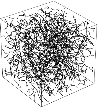
All simulations are initiated with a random configuration of vortex rings which seed the turbulence. As with previous studies, after and initial transient, the vortex line density $L=\Lambda/V$ (defined as the superfluid vortex length $\Lambda=\int_{\cal L}d\xi$ in the volume $V={\cal D}^{3}$) saturates to a quasi-steady state (independent of the initial seed) such that energy input from the driving normal fluid is balanced by dissipation due to friction and vortex reconnections. The intervortex distance is estimated as $\ell\approx L^{-1/2}$. A typical vortex tangle is displayed in Fig. 1. Within the saturated regime we compute velocity and acceleration statistics, using stored velocity information at the discretization points ${\bf{s}}_{i}$ via a fourth-order upwind finite–difference scheme

$$\mathbf{a}_{i}^{n}=\dfrac{-{\bf{v}}_{i}^{n-3}+6{\bf{v}}_{i}^{n-2}-18{\bf{v}}_{i}^{n-1}+10{\bf{v}}_{i}^{n}+3{\bf{v}}_{i}^{n+1}}{\Delta t},$$ (3)

where $\mathbf{a}_{i}^{n}$ is the acceleration of the $i^{\rm th}$ vortex point at the $n^{\rm th}$ time step and ${\bf{v}}_{i}^{n}=d{\bf{s}}_{i}^{n}/dt$ is the velocity of the $i^{\rm th}$ vortex point at the $n^{\rm th}$ time step, computed using Eq. (1). What we measure thus represents the Lagrangian acceleration of ideal point tracers which are trapped in vortex lines (hence are affected by friction), but are unaffected by Stokes drag.

Figure 1: A snapshot of the vortex configuration (plotted as black space curves) at T=1.75 K, $v_{ns}=1~{}\rm cm/s$, during the quasi-steady state regime. Vortex line density $L=15750~{}\rm cm^{-2}$, estimated intervortex distance $\ell\approx 0.008~{}\rm cm$.

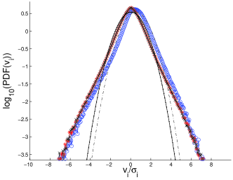
First we consider the velocity. PDFs of the velocity components $v_{x}$, $v_{y}$ and $v_{z}$ of ${\bf{v}}_{i}$ from the simulation at T=1.75 K, $v_{ns}=1\,$cm/s, which are plotted in Fig. 2. Note the power–law behavior of the tails. Best–fits to the data give PDF$(v)\propto v^{-3.2}$; comparable results are obtained at different $T$ and $v_{ns}$. The PDF’s exponents, close to $-3$, are the tell–tale signature of quantum turbulence, and can be understood if we consider an isolated straight vortex line (the effect of adding the contributions of many vortices is discussed in ref. White10 ). The argument is the following. At the distance $r$ from its axis, the vortex line induces a velocity field $v\propto 1/r$. The probability $P(v)dv$ of finding the value $v$ is thus proportional to the area $2\pi rdr$ of the annulus between $r$ and $r+dr$; therefore $P(v)dv\sim rdr\sim(1/v)(dv/v^{2})\sim v^{-3}dv$, hence ${\rm PDF}(v)\sim v^{-3}$, in agreement with experiments paoletti2008velocity and numerical studies Baggaley-stats .

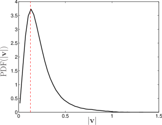
It is also instructive to examine $|{\bf{v}}_{i}|$, the modulus of the velocity ${\bf{v}}_{i}$. Numerical experiments Sherwin2012 confirm the heuristic argumentVinen-Niemela that counterflow turbulence is featureless (compared with classical turbulence), and the vortex tangle is characterized by the single length scale $\ell$. The prominent peak of PDF($|{\bf{v}}|$) displayed in Fig. 3 corresponds to the velocity scale $\kappa/\ell\approx 0.13~{}\rm cm/s$, lending further weight to the argument. The mean of the distribution, $\langle|\mathbf{v}|\rangle=0.23~{}\rm cm/s$, is close to the characteristic velocity of a vortex line rotating around another line, $v_{\ell}=\kappa/(\ell/2)\approx 0.25~{}\rm cm/s$.

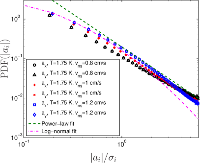
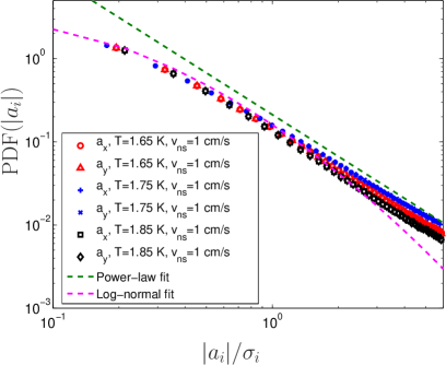
We turn now the attention to the acceleration. Fig. 4 displays statistics of the modulus of the $x$ and $y$-components ($a_{x}$ and $a_{y}$) of the acceleration $\mathbf{a}_{i}$, normalized by the corresponding standard deviations ($\sigma_{x}$ and $\sigma_{y}$). The statistics for $a_{z}$ are indistinguishable from those of $a_{y}$. This is not surprising, because $x$ is the longitudinal direction of the counterflow, and the two transversal directions, $y$ and $z$, are equivalent. It is interesting to notice that the acceleration statistics are not affected by the mild anisotropy of counterflow (for example, at $T=1.75~{}\rm K$ and $v_{ns}=1~{}\rm cm/s$, the projected vortex lengths are such that $L_{x}/L=0.37,L_{y}/L=L_{z}/L=0.54$.

The results displayed in Fig. 4 are computed at fixed temperature ($T=1.75~{}\rm K$) and varying counterflow velocities $v_{ns}$ (left), and at fixed counterflow velocity ($v_{ns}=1~{}\rm cm/s$) and varying temperatures (right). In either cases we can fit both a log-normal distribution to the data, and a power law to the tails of the PDF for large accelerations. If we apply the straight vortex line argument to the acceleration $a=v^{2}/r$, we find that the probability of the value $a$ is $P(a)da\sim rdr\sim(1/a^{1/3})(da/a^{4/3})\sim a^{-5/3}da$, hence we expect ${\rm PDF}(a)\sim a^{-5/3}$. The exponents shown in Fig. 4 are in general more shallow than -5/3. A possible explanation is that vortex reconnections increase the probability of large accelerations. Lognormal distributions are heavy-tailed (i.e. the tails of the distribution are not exponentially bounded), and show reasonable agreement with the data, as found by La Mantia LaMantia . However it is clear that we observe a power-law scaling for the acceleration statistics in this study, with good agreement to the predicted $-5/3$ scaling.

We now consider the mean value $\langle|\mathbf{a}|\rangle$ of the acceleration. The previous argument suggests that the characteristic acceleration of a vortex line rotating around another line is of the order of $a_{\ell}=v_{\ell}^{2}/(\ell/2)=8\kappa^{2}/\ell^{3}$. La Mantia’s experiments support this estimate. La Mantia reports that (insets of figure 1 of ref. LaMantia ) that $\langle|\mathbf{a}|\rangle\approx 3.2$ and $1.9~{}\rm cm/s^{2}$ respectively at $T=1.64~{}K$, $\dot{Q}=586~{}\rm W/m^{2}$ and at $T=1.86~{}K$, $\dot{Q}=595~{}\rm W/m^{2}$. If we relate the heat flux to the counterflow velocity (via $v_{ns}={\dot{Q}}/(\rho_{s}ST)$ where $S$ and $\rho_{s}$ are the specific entropy and the superfluid density), the counterflow velocity to the vortex line density (via $L=\gamma^{2}v_{ns}^{2}$, where $\gamma$ was calculated by Adachi Adachi2010 ), and the vortex line density to the characteristic vortex distance (via $\ell\approx L^{-1/2}$), we find $a_{\ell}\approx 3.3$ and $1.1~{}\rm cm/s^{2}$ respectively, in order of magnitude agreement with La Mantia’s measurements of $\langle|\mathbf{a}|\rangle$. The estimate $a_{\ell}$ also agrees with the numerical simulations. For example, at $T=1.75~{}\rm K$, $v_{ns}=1~{}\rm cm/s$ we find $a_{\ell}\approx 16~{}\rm cm/s^{2}$ which compares well with mean, median and mode of the computed distribution, which are $72$, $35$ and $10~{}\rm cm/s^{2}$ respectively.

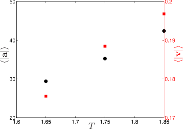
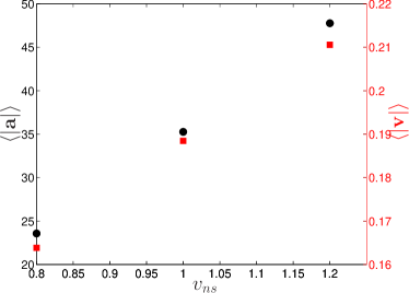
Finally, Fig. 5 shows that both velocity and acceleration increase with temperature $T$ (at fixed counterflow velocity $v_{ns}$) and with $v_{ns}$ (at fixed $T$). La Mantia reports that $\langle|\mathbf{a}|\rangle$ increases with heat flux $\dot{Q}$ (at fixed $T$), but decreases with $T$ (at fixed $\dot{Q}$). There is no disagreement between La Mantia’s results and ours. In fact, on one hand we can write $a_{\ell}=8\kappa^{2}/\ell^{2}=8\kappa^{2}\gamma^{2}v_{ns}^{3}$: this relation and the fact that $\gamma$ increases with increasing $T$ Adachi2010 , explains why in the numerical simulations $\langle|\mathbf{a}|\rangle$ increases with $v_{ns}$ (at fixed $T$) and increases with $T$ (at fixed $v_{ns}$). On the other hand we can also write $a_{\ell}=8\kappa^{2}(\gamma{\dot{Q}}/(\rho ST))^{3}$: this relation accounts for La Mantia’s observations that $\langle|\mathbf{a}|\rangle$ increases with $\dot{Q}$ (at fixed $T$) but decreases with $T$ (at fixed $\dot{Q}$) because the quantity $\gamma/(\rho_{s}ST)$ decreases with increasing $T$ Donnelly1998 ; Adachi2010 .

Our results shed light onto the complex dynamics of tracer particles. Consider a particle of radius $a_{p}$, velocity ${\bf{v}}_{p}$ and density $\rho_{p}$ which is not trapped into vortices and moves in helium II. Assuming a steady uniform normal fluid, its acceleration is due to Stokes drag and inertial effects Poole :

$$\frac{d{\bf{v}}_{p}}{dt}=\frac{9\mu_{n}({\bf{v}}_{n}-{\bf{v}}_{p})}{2\rho_{0}a_{p}^{2}}+\frac{3\rho_{s}}{2\rho_{0}}\frac{D{\bf{v}}_{s}}{Dt},$$ (4)

where $\rho$ and $\mu_{n}$ are helium’s density and viscosity, and $\rho_{0}=\rho_{p}+\rho/2$. The Stokes drag (which pulls the particle along the normal fluid) has magnitude of the order of $9\beta\mu_{n}v_{n}/(2\rho_{0}a_{p}^{2})$ where $v_{n}=\rho_{s}v_{ns}/\rho$, $\beta v_{n}$ is the average slip velocity and $0<\beta<1$; unfortunately we do not know $\beta$ and we cannot predict the relative importance of the two contributions to $d{\bf{v}}_{p}/dt$. Temporal variations of ${\bf{v}}_{s}$ become important only after the particle has collided with a vortex and triggered Kelvin waves Kivotides2008 , hence, for a free particle, the inertial term (which pulls the particle towards the nearest vortex, effectively a radial pressure gradient) becomes $D{\bf{v}}_{s}/DT=\partial{\bf{v}}_{s}\partial t+({\bf{v}}_{s}\cdot\nabla){\bf{v}}_{s}\approx({\bf{v}}_{s}\cdot\nabla){\bf{v}}_{s}$; its magnitude is of the order of $v_{s}^{2}/(\ell/2)=a_{\ell}$ (which we interpreted as the acceleration of a particle trapped into a vortex which rotates around another vortex). In La Mantia’s experiment $\rho_{0}\approx 1.9\rho$, so the prefactor in front of the inertial term is of order unity. The order of magnitude agreement between the observed acceleration and our estimate $a_{\ell}$ suggests that the Stokes term is less important than the inertia term. We can now interpret $a_{\ell}$ as either the acceleration of a particle trapped into a vortex which rotates around another vortex, of the fluctuating pressure grandient which attracts a free particle to a vortex line.

Figure 2: (Color online) Probability density functions (PDF) of turbulent velocity components $v_{i}$ ($i=x,y,z)$ vs $v_{i}/\sigma_{i}$ computed from the velocity of the vortex points $d{\bf{s}}_{i}/dt$ from the simulation corresponding to Fig. 1 ($T=1.75~{}\rm K$, $v_{ns}=1~{}\rm cm/s$). (Blue) circles, (red) asterisks and (black) crosses refer respectively to $i=x$, $i=y$ and $i=z$ components. Gaussian fits, ${\rm gPDF}(v_{i})=\frac{1}{\sqrt{2\pi\sigma^{2}}}{\rm exp}(-(v_{i}-\mu)^{2}/(2\sigma^{2}))$ for each component ($i=x$: dot-dashed line; $i=y$: solid line, $i=z$: solid points) are plotted to emphasize the deviation from Gaussianity. Here $\sigma_{x}=0.1162$, $\sigma_{y}=0.1148$, and $\sigma_{z}=0.1156$.

Figure 3: The probability density function (PDF) of the modulus of the velocity $|\mathbf{v}|$; the dashed (red) lines represents the ‘characteristic’ velocity, $\kappa/\ell$. The PDF is computed from the data in Fig. 2 ($T=1.75~{}\rm K$, $v_{ns}=1~{}\rm cm/s$).

Figure 4: PDFs of the $x$ and $y$ components of the acceleration of the quantized vortices, scaled by the standard deviation of the relevant component. Left, at fixed temperature, with increasing counterflow velocity, right, varying the temperature with a fixed counterflow velocity. Log normal and power law (PDF$\sim a_{i}^{-5/3}$) fits to the data are plotted. Power law fits to the data yield PDF$(|a_{i}|/\sigma_{i})\sim(a_{i}/\sigma_{i})^{\beta}$ ; $\beta=-1.48$, T=1.75  K, $v_{ns}=0.8\,$ cm/s ; $\beta=-1.64$, T=1.75  K, $v_{ns}=1\,$ cm/s ; $\beta=-1.71$, T=1.75  K, $v_{ns}=1.2\,$ cm/s ; $\beta=-1.55$, T=1.65  K, $v_{ns}=1\,$ cm/s ; $\beta=-1.58$, T=1.75  K, $v_{ns}=1\,$ cm/s ; $\beta=-1.63$, T=1.85  K, $v_{ns}=1\,$ cm/s.

Figure 5: Dependence of median velocity, $\langle{|\mathbf{v}|}\rangle$ ($\rm cm/s$), and acceleration, $\langle{|\mathbf{a}|}\rangle$ ($\rm cm/s^{2}$), on temperature $T$ (left, in $\rm K$) and counterflow velocity $v_{ns}$ (right, in $\rm cm/s$). In each panel, the left axis and (black) circles correspond to acceleration, and the right axis and (red) squares correspond to velocity.

In conclusion, we have numerically determined the one–point superfluid acceleration statistics in counterflow turbulence, and demonstrated how mean velocity and acceleration scale with counterflow velocity and temperature. The importance of our results springs from the fact that La Mantia did not measure directly the superfluid acceleration or the vortex acceleration, but rather the acceleration of micron–sized solid hydrogen particles, whose dynamics is complex Poole ; Kivotides2008 . The good agreement between our findings and La Mantia’s in terms of acceleration statistics means that this difference is not crucial. We also argue that the probability density function of one–point acceleration statistics should follow a power law distribution, with a $-5/3$ exponent. Our numerical results support these arguments.

The results reported by La Mantia did not distinguish between particles which are trapped in vortices (hence move along the imposed superflow) and particles which are free (hence move along the normal fluid). Separate analysis of acceleration statistics of these two groups of particles will be useful. Theoretically, an approach which accounts reasonably well for velocity and acceleration statistics in classical turbulence is the multifractal formalism Biferale2004 , which in principle could be adapted to model quantum turbulence.

C.F.B. is grateful to the EPSRC for grant number EP/I019413/1.

References

- (1) W. F. Vinen, Proceedings of the Royal Society of London. Series A. Mathematical and Physical Sciences 240, 114 (1957).
- (2) W. F. Vinen, Proceedings of the Royal Society of London. Series A. Mathematical and Physical Sciences 240, 128 (1957).
- (3) W. F. Vinen, Proceedings of the Royal Society of London. Series A. Mathematical and Physical Sciences 242, 493 (1957).
- (4) W. F. Vinen, Proceedings of the Royal Society of London. Series A. Mathematical and Physical Sciences 243, 400 (1958).
- (5) D. I. Bradley, S. N. Fisher, A. M. Guénault, R. P. Haley, S. O’Sullivan, G. R. Pickett, and V. Tsepelin, Phys. Rev. Lett. 101, 065302 (2008).
- (6) E. A. L. Henn, J. A. Seman, G. Roati, K. M. F. Magalhães, and V. S. Bagnato, Phys. Rev. Lett. 103, 045301 (2009).
- (7) R. Donnelly, Quantized Vortices in Helium II, Cambridge University Press, 1991.
- (8) G. Bewley, M. Paoletti, S. Sreenivasan, and D. Lathrop, PNAS 105, 13707 (2008).
- (9) M. S. Paoletti, M. E. Fisher, K. R. Sreenivasan, and D. P. Lathrop, Phys. Rev. Lett. 101, 154501 (2008).
- (10) A. C. White, C. F. Barenghi, N. P. Proukakis, A. J. Youd, and D. H. Wacks, Phys. Rev. Lett. 104, 075301 (2010).
- (11) A. Baggaley and C. Barenghi, Phys. Rev. B 84, 067301 (2011).
- (12) N. Mordant, A. M. Crawford, and E. Bodenschatz, Phys. Rev. Lett. 93, 214501 (2004).
- (13) A. M. Crawford, N. Mordant, and E. Bodenschatz, Phys. Rev. Lett. 94, 024501 (2005).
- (14) M. La Mantia, D. Duda, M. Rotter, and L. Skrbek, Journal of Fluid Mechanics 717 (2013).
- (15) D. Kivotides, C. Barenghi, and Y. Sergeev, Physical Review B 77, 014527 (2008).
- (16) K. W. Schwarz, Phys. Rev. B 31, 5782 (1985).
- (17) R. J. Donnelly and C. F. Barenghi, J. Phys. Chem. Ref. Data 27, 1217 (1998).
- (18) P. Saffman, Vortex Dynamics, Cambridge Monographs on Mechanics, Cambridge University Press, 1995.
- (19) A. Baggaley and C. Barenghi, Journal of Low Temperature Physics 166, 3 (2012).
- (20) A. Baggaley, J. Low Temp. Phys. 168, 18 (2012).
- (21) H. Adachi, S. Fujiyama, and M. Tsubota, Phys. Rev. B 81, 104511 (2010).
- (22) A. W. Baggaley, L. K. Sherwin, C. F. Barenghi, and Y. A. Sergeev, Phys. Rev. B 86, 104501 (2012).
- (23) W. Vinen and J. Niemela, J. Low Temp. Physics 128, 167 (2000).
- (24) The PDF of the log-normal distribution is given by PDF()=, where is the mean of the distribution and is the variance.
- (25) D. R. Poole, C. F. Barenghi, Y. A. Sergeev, and W. F. Vinen, Phys. Rev. B 71, 064514 (2005).
- (26) L. Biferale, G. Boffetta, A. Celani, B. J. Devenish, A. Lanotte, and F. Toschi, Phys. Rev. Lett. 93, 064502 (2004).