Uniform Error Estimation for Convection-Diffusion Problems

[n]

Acknowledgement

Abstract

Let us consider the singularly perturbed model problem

$$Lu:=-\varepsilon\Delta u-bu_{x}+cu =f$$

with homogeneous Dirichlet boundary conditions on $$\Gamma=\partial\Omega$$

$$u|_{\Gamma} =0$$

on the unit-square $\Omega=(0,1)^{2}$. Assuming that $b>0$ is of order one, the small perturbation parameter $0<\varepsilon\ll 1$ causes boundary layers in the solution.

In order to solve above problem numerically, it is beneficial to resolve these layers. On properly layer-adapted meshes we can apply finite element methods and observe convergence.

We will consider standard Galerkin and stabilised FEM applied to above problem. Therein the polynomial order $p$ will be usually greater then two, i.e. we will consider higher-order methods.

Most of the analysis presented here is done in the standard energy norm. Nevertheless, the question arises: Is this the right norm for this kind of problem, especially if characteristic layers occur? We will address this question by looking into a balanced norm.

Finally, a-posteriori error analysis is an important tool to construct adapted meshes iteratively by solving discrete problems, estimating the error and adjusting the mesh accordingly. We will present estimates on the Green’s function associated with $L$, that can be used to derive pointwise error estimators.

Chapter 1 Introduction

Simple model problems are often helpful in understanding the behaviour of numerical methods in presence of layers for more complicated problems. We will consider the singularly perturbed convection-diffusion problem with an exponential layer at the outflow boundary and two characteristic layers, given by

$$-\varepsilon\Delta u-bu_{x}+cu =f \text{in}\ \Omega=(0,1)^{2},$$ (1.1a)

$$u =0 \text{on}\ \partial\Omega.$$ (1.1b)

We assume $f\in C(\bar{\Omega})$, $b\in W^{1}_{\infty}(\bar{\Omega})$ and $c\in L_{\infty}(\bar{\Omega})$. Furthermore, let $b(x,y)\geq\beta$ for $(x,y)\in\bar{\Omega}$ with some positive constant $\beta$ of order one, while $0<\varepsilon\ll 1$ is a small perturbation parameter. For further assumptions on $f$ see Remark 2.2.

This combination gives rise to an exponential layer of width $\mathcal{O}\left(\varepsilon|\ln\varepsilon|\right)$ at $x=0$ and to two characteristic layers of width $\mathcal{O}\left(\sqrt{\varepsilon}|\ln\varepsilon|\right)$ at $y=0$ and $y=1$. Figure 1.1

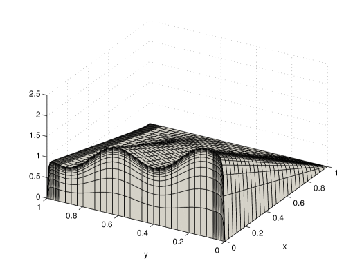
Figure 1.1: Typical solution of (1.1) with two parabolic layers and an exponential layer.

shows a typical example of a solution $u$ to (1.1).

Under the condition

$$c+\textstyle\frac{1}{2}b_{x}\geq\gamma>0$$ (1.2)

problem (1.1) possesses a unique solution in $H^{1}_{0}(\Omega)\cap H^{2}(\Omega)$. Note that (1.2) can always be satisfied by a transformation $\tilde{u}(x,y)=u(x,y)e^{\varrho x}$ with a suitably chosen constant $\varrho$. In our case $\varrho$ with $\varrho(b-\varepsilon\varrho)\geq c+\frac{1}{2}b_{x}+\gamma$ suffices.

When quasi uniform meshes are used, numerical methods do not give accurate approximations of (1.1) unless the mesh size is of the order of the perturbation parameter $\varepsilon$. On the one hand this constitutes a prohibitive restriction for a practical treatment of singularly perturbed problems. But on the other hand, the mesh sizes do only have to be small in the layer region. Therefore, layer-adapted meshes are often used to obtain efficient discretisations.

Based on a priori knowledge of the layer behaviour, we apply a-priori adapted meshes. Early ideas on layer-adapted meshes can be found in [4, 48, 55, 61]. We will use generalisations of Shishkin meshes, so called S-type meshes [52, 40, 41], that resolve the layers and yield robust (or uniform) convergence.

In Figure 1.1 the layer-resolving effect of Shishkin’s idea can be seen clearly. We have condensed meshes near the characteristic boundaries ($y=1$ and $y=0$, resp.) and the outflow boundary ($x=0$).

Even on layer-adapted meshes the standard Galerkin method shows instabilities, see [42, 58]. Therefore, stabilised discretisations have to be considered. The recent book by Roos, Stynes and Tobiska [54] gives an overview of many stabilisation ideas.

We will apply and analyse two stabilisation techniques. The first one will be the streamline-diffusion finite element method (SDFEM), introduced by Hughes and Brooks [29]. For problems with characteristic layers, the SDFEM with bilinear elements was analysed in [22]. Here we will look into higher-order finite element methods. A disadvantage of the SDFEM accounts in particular for discretisations with higher-order elements. Several additional terms like second order derivatives have to be assembled in order to ensure Galerkin orthogonality of the resulting method.

The second stabilisation technique does not fulfil the Galerkin orthogonality. It is the Local Projection Stabilisation method, proposed originally for the Stokes problem in [5]. Although, the Galerkin orthogonality is not valid, the remainder can be bounded such that the optimal order of convergence is maintained. Again, we will look into higher-order methods.

The main focus of our analysis will be the uniform convergence and supercloseness of the numerical methods with respect to $\varepsilon$. Most of it is done in the so-called energy norm

$$\left|\!\!\;\left|\!\!\;\left|{v}\right|\!\!\;\right|\!\!\;\right|_{\varepsilon}:=\left(\varepsilon\|{\nabla v}\|_{0}^{2}+\gamma\|{v}\|_{0}^{2}\right)^{1/2}.$$ (1.3)

We denote by $\|{\cdot}\|_{L_{p}(D)}$ the standard $L_{p}$-norm over $D\subset\mathbb{R}^{2}$. Whenever $p=2$ we write $\|{\cdot}\|_{0,D}$ and if $D=\Omega$ we skip the reference to the domain.

Not all norms are equally adequate in measuring errors for problems with layers. Although the energy-norm is the associated norm to the weak formulation of (1.1), not all features of the solution are “seen”. Especially for small $\varepsilon$ the characteristic layer term is less represented then the exponential one. Therefore,s we will also consider a balanced norm, where both types of layer are equally well represented.

Another norm that is suitable in recognising the layer behaviour is the $L_{\infty}$-norm. We will not present a-priori results in the maximum-norm but an approach to uniform pointwise a-posteriori error estimation using the Green’s function.

This habilitation treatise is structured as follows. In Chapter 2 the basics are given, i.e. a solution decomposition of $u$ is assumed, meshes, polynomial spaces and interpolation operators defined, and finally the numerical methods are given. In Chapter 3 we present several analytical and numerical results on the convergence and supercloseness of the numerical methods in the energy and related norms. In Chapter 4 we consider the question, whether a different norm then the energy norm could and should be used in the analysis. Finally, in Chapter 5 we present $L_{1}$-norm estimates of the Green’s function associated with problems like (1.1). Moreover, they are applied in a first a-posteriori error-estimator for a simple finite difference method.

Most of the results of the Chapters 2-5 are from already published work. Eight of the papers, whose content is contained in these chapters, are given in the appendix.

Notation. Throughout this treatise, $C$ denotes a generic constant that is independent of both the perturbation parameter $\varepsilon$ and the mesh parameter $N$. The dependence of any constant on the polynomial order $p$ will not be elaborated.

Chapter 2 Meshes and Numerical Methods

This chapter contains results from [23, 24, 16] that are also given in Appendix Appendix, Appendix and Appendix.

2.1 Solution Decomposition

Our uniform numerical analysis is based on a decomposition of the solution $u$ of (1.1). To be more precise: We suppose the existence of a decomposition of $u$ into a regular solution component and various layer parts.

Assumption 2.1.

The solution $u$ of problem (1.1) can be decomposed as

$$u=v+w_{1}+w_{2}+w_{12},$$

where we have for all $x,y\in[0,1]$ and $0\leq i+j\leq p+1$ the pointwise estimates

$$\left.\begin{aligned} \left|\frac{\partial^{i+j}v}{\partial x^{i}\partial y^{j}}(x,y)\right|&\leq C,\quad\left|\frac{\partial^{i+j}w_{1}}{\partial x^{i}\partial y^{j}}(x,y)\right|\leq C\varepsilon^{-i}e^{-\beta x/\varepsilon},\\[5.69046pt] \left|\frac{\partial^{i+j}w_{2}}{\partial x^{i}\partial y^{j}}(x,y)\right|&\leq C\varepsilon^{-j/2}\left(e^{-y/\sqrt{\varepsilon}}+e^{-(1-y)/\sqrt{\varepsilon}}\right),\\[5.69046pt] \left|\frac{\partial^{i+j}w_{12}}{\partial x^{i}\partial y^{j}}(x,y)\right|&\leq C\varepsilon^{-(i+j/2)}e^{-\beta x/\varepsilon}\left(e^{-y/\sqrt{\varepsilon}}+e^{-(1-y)/\sqrt{\varepsilon}}\right).\end{aligned}\right\}$$ (2.1)

Here $w_{1}$ is the exponential boundary layer, $w_{2}$ covers the characteristic boundary layers, $w_{12}$ the corner layers, and $v$ is the regular part of the solution.

Remark 2.2.

The validity of Assumption 2.1 is proved in [31, 32] for constant functions $b,\,c$ under certain compatibility and smoothness conditions on the right-hand side $f$.

In [19] the Green’s function associated with problem (1.1) was analysed. It was shown, that the Green’s function $G$ in the variable-coefficient case and the Green’s function $\bar{G}$ in the constant coefficient case show a similar behaviour and the same estimates. As a Green’s function can be used to represent the solution $u$ of its associated problem by

$$u(x,y)=\iint_{\Omega}G(x,y;\xi,\eta)f(\xi,\eta)d\xi d\eta,$$

it is reasonable to assume the validity of Assumption 2.1 in the variable-coefficient case too.

2.2 Layer-Adapted Meshes

A discretisation of a singularly perturbed problem on an equidistant mesh results in oscillatory solutions unless the mesh-size is of order $\varepsilon$. A loophole lies in layer-adapted meshes that are fine in layer regions and coarse in regions, where the solution and its derivatives are uniformly bounded.

Back in 1969 Bakhvalov [4] proposed one of the first layer-adapted meshes. Analysis on these kinds of graded meshes is somewhat difficult. The piecewise uniform Shishkin meshes [48] proposed in 1996 are easier to handle. The first analysis of finite element methods on Shishkin meshes was published in [55]. For a detailed discussion of properties of Shishkin meshes and their uses see [54] and also [41] for a survey on layer-adapted meshes.

Here we use a tensor-product mesh that is constructed by taking in both $x$- and $y$-direction so called S-type meshes [52] with $N$ mesh intervals in each direction. These meshes condense in the layer regions and are equidistant outside the layer region. The points, where the mesh-character changes, are called transition points. We define them by

$$\lambda_{x}:=\frac{\sigma\varepsilon}{\beta}\ln N\leq\frac{1}{2}\quad\text{and}\quad\lambda_{y}:=\sigma\sqrt{\varepsilon}\ln N\leq\frac{1}{4},$$ (2.2)

with some user-chosen positive parameter $\sigma>0$. In (2.2) we assumed

$$\varepsilon\leq\min\left\{\frac{\beta}{2\sigma}(\ln N)^{-1},\frac{1}{16\sigma^{2}}(\ln N)^{-2}\right\}\leq C(\ln N)^{-2}$$ (2.3)

which is typically for (1.1) as otherwise $N$ would be exponentially large in $\varepsilon$.

Using these transition points, the domain $\Omega$ is divided into the subdomains $\Omega_{11}$, $\Omega_{12}$, $\Omega_{21}$ and $\Omega_{22}$ as shown in Fig. 2.1. Here $\Omega_{12}$ covers the exponential layer, $\Omega_{21}$ the characteristic layers, $\Omega_{22}$ the corner layers and $\Omega_{11}$ the remaining non-layer region.

$$\Omega_{11} :=[\lambda_{x},1]\times[\lambda_{y},1-\lambda_{y}],$$

$$\Omega_{12} :=[0,\lambda_{x}]\times[\lambda_{y},1-\lambda_{y}],$$

$$\Omega_{21} :=[\lambda_{x},1]\times\big{(}[0,\lambda_{y}]\cup[1-\lambda_{y},1]\big{)},$$

$$\Omega_{22} :=[0,\lambda_{x}]\times\big{(}[0,\lambda_{y}]\cup[1-\lambda_{y},1]\big{)}$$

Figure 2.1: Decomposition of $\Omega$ into subregions.

By choosing the transition points $\lambda_{x}$ and $\lambda_{y}$ according to (2.2), the layer terms $w_{1}$, $w_{2}$, and $w_{12}$ of $u$ are of size $\mathcal{O}\left(N^{-\sigma}\right)$ on $\Omega_{11}$, i.e.,

$$\big{|}w_{1}(x,y)\big{|}+\big{|}w_{2}(x,y)\big{|}+\big{|}w_{12}(x,y)\big{|}\leq CN^{-\sigma}\quad\text{for}\ (x,y)\in\Omega_{11}.$$

The parameter $\sigma$ is typically equal to the formal order of the numerical method or is chosen slightly larger to accommodate the error analysis. The precise definition of $\sigma$ will be given later.

The domain $\Omega_{11}$ will be dissected uniformly while the dissection in the other subdomains depends on the mesh generating function $\phi$. This function is monotonically increasing and satisfies $\phi(0)=0$ and $\phi(1/2)=\ln N$. The precise definition of the tensor product mesh $T^{N}$ is given by the mesh points

$$x_{i} :=\begin{cases}\frac{\sigma\varepsilon}{\beta}\phi\left(\frac{i}{N}\right),&i=0,\dots,N/2,\\ 1-2(1-\lambda_{x})(1-\frac{i}{N}),&i=N/2,\dots,N,\end{cases}$$

$$y_{j} :=\begin{cases}\sigma\sqrt{\varepsilon}\phi\left(\frac{2j}{N}\right),&j=0,\dots,N/4,\\ \frac{1}{2}+(1-2\lambda_{y})(\frac{2j}{N}-1),&j=N/4,\dots,3N/4,\\ 1-\sigma\sqrt{\varepsilon}\phi\left(2-\frac{2j}{N}\right),&j=3N/4,\dots,N.\end{cases}$$

Now with an arbitrary function $\phi$ fulfilling above conditions, an S-type mesh is defined.

Figure 2.2: Layer-adapted mesh $T^{8}$ of $\Omega$.

Fig. 2.2 shows an example of such a mesh.

Related to the mesh-generating function $\phi$, we define by

$$\psi=\mathrm{e}^{-\phi}$$

the mesh-characterising function $\psi$ which is monotonically decreasing with $\psi(0)=1$ and $\psi(1/2)=N^{-1}$.

In Table 2.1 some representatives of S-type meshes from [52] are given. The polynomial S-mesh has an additional parameter $m>0$ to adjust the grading inside the layer.

Table 2.1: Some examples of mesh-generating and mesh-characterising functions of S-type meshes.

Name	$\phi(t)$	$\max\phi^{\prime}$	$\psi(t)$	$\max|\psi^{\prime}|$
Shishkin mesh	$2t\ln N$	$2\ln N$	$N^{-2t}$	$2\ln N$
Bakhvalov S-mesh	$-\!\ln(1\!-\!2t(1\!-\!N^{-1}))$	$2N$	$1\!-\!2t(1\!-\!N^{-1})$	2
polynomial S-mesh	$(2t)^{m}\ln N$	$2m\ln N$	$N^{-(2t)^{m}}$	$C(\ln N)^{1/m}$
modified Bakhvalov S-mesh	$\frac{t}{q-t},\,q=\frac{1}{2}(1+\frac{1}{\ln N})$	$3\ln^{2}N$	$\mathrm{e}^{-\frac{t}{q-t}}$	$3/(2q)\leq 3$

In order to provide sufficient properties for our convergence analysis, the meshes need to fulfil some additional assumptions.

Assumption 2.3.

Let the mesh-generating function $\phi$ be piecewise differentiable such that

$$\max_{t\in[0,\frac{1}{2}]}\phi^{\prime}(t)\leq CN\,\text{ or equivalently }\max_{t\in[0,\frac{1}{2}]}\frac{|\psi^{\prime}(t)|}{\psi(t)}\leq CN$$ (2.4)

is fulfilled. Moreover, let $\phi$ fulfil

$$\min_{i=0,\dots,N/2-1}\left(\phi\left(\frac{i+1}{N}\right)-\phi\left(\frac{i}{N}\right)\right)\geq CN^{-1}.$$ (2.5)

Finally we assume

$$\max|\psi^{\prime}|:=\max_{t\in[0,\frac{1}{2}]}|\psi^{\prime}(t)|\leq C\left(\frac{N}{\ln N}\right)^{1/2}.$$ (2.6)

Remark 2.4.

Note that (2.4) is satisfied for all meshes given in Table 2.1. Assumption (2.5) allows to bound the mesh width in the layer regions from below while applying an inverse inequality. This additional assumption restricts the use of S-type meshes from Table 2.1. For the original Shishkin mesh, we have

$$\min_{i=0,\dots,N/2-1}\left(\phi\left(\frac{i+1}{N}\right)-\phi\left(\frac{i}{N}\right)\right)=CN^{-1}\ln N\geq CN^{-1}.$$

The Bakhvalov S-mesh and its modification both fulfil

$$\min_{i=0,\dots,N/2-1}\left(\phi\left(\frac{i+1}{N}\right)-\phi\left(\frac{i}{N}\right)\right)\geq CN^{-1}.$$

But the polynomial S-type mesh yields

$$\min_{i=0,\dots,N/2-1}\left(\phi\left(\frac{i+1}{N}\right)-\phi\left(\frac{i}{N}\right)\right)\geq CN^{-m}$$

such that Assumption (2.5) fails for $m>1$.

The restriction (2.6) is fulfilled for all meshes of Table 2.1. Nevertheless, S-meshes fulfilling the other two assumptions such that (2.6) is violated are possible, see [23, Remark 14]. The quantity $1+(N^{-1}\ln N)^{1/2}\max|\psi^{\prime}|$ arises in the convergence analysis of the Galerkin FEM, see [23], and can be bounded by a constant $C$ with the help of (2.6).

Using (2.4) we bound the mesh width inside the layers from above. Let $h_{i}:=x_{i}-x_{i-1}$ and $t_{i}=i/N$. Then, it holds for $i=1,\dots,N/2$ and $t\in[t_{i-1},t_{i}]$ (with $\max\phi^{\prime}$ taken over $t\in[t_{i-1},t_{i}]$)

$$\psi(t_{i})=\mathrm{e}^{-\phi(t_{i})}=\mathrm{e}^{-(\phi(t_{i})-\phi(t))}\mathrm{e}^{-\phi(t)} \geq\mathrm{e}^{-(\phi(t_{i})-\phi(t_{i-1}))}\psi(t)$$ (2.7)

$$\geq\mathrm{e}^{-N^{-1}\max\phi^{\prime}}\psi(t)\geq C\psi(t)$$

where we used (2.4) for the last estimate. Furthermore, we have

$$x=\frac{\sigma\varepsilon}{\beta}\phi(t)=-\frac{\sigma\varepsilon}{\beta}\ln\psi(t)\quad\mbox{which gives}\quad\psi(t)=\mathrm{e}^{-\beta x/(\sigma\varepsilon)}.$$

Using this, the monotonicity of $\psi$, and (2.7), we obtain for $i=1,\ldots,N/2$ and $x\in[x_{i-1},x_{i}]$

$$h_{i} =\frac{\sigma\varepsilon}{\beta}(\phi(t_{i})-\phi(t_{i-1}))\leq\frac{\sigma}{\beta}\varepsilon N^{-1}\max_{t\in[t_{i-1},t_{i}]}\phi^{\prime}(t)\leq\frac{\sigma}{\beta}\varepsilon N^{-1}\left(\max_{t\in[t_{i-1},t_{i}]}|\psi^{\prime}(t)|\right)/\psi(t_{i})$$

$$\leq C\varepsilon N^{-1}\left(\max_{t\in[t_{i-1},t_{i}]}|\psi^{\prime}(t)|\right)/\psi(t)\leq C\varepsilon N^{-1}\max|\psi^{\prime}|\mathrm{e}^{\beta x/(\sigma\varepsilon)}$$ (2.8)

where again $\max|\psi^{\prime}|:=\max\limits_{t\in[0,1/2]}|\psi^{\prime}(t)|$.
Similarly, we get for $j=1,\dots,N/4$ and $j=3N/4+1,\dots,N$

$$k_{j}:=y_{j}-y_{j-1} \leq C\varepsilon^{1/2}N^{-1}\max|\psi^{\prime}|\begin{cases}\mathrm{e}^{y/(\sigma\varepsilon^{1/2})},&j\leq N/4,\\ \mathrm{e}^{(1-y)/(\sigma\varepsilon^{1/2})},&j>3N/4,\end{cases}$$ (2.9)

with $y\in[y_{j-1},y_{j}]$. Of course, the simpler bounds

$$h_{i} \leq C\varepsilon N^{-1}\max\phi^{\prime} \leq C\varepsilon, i=1,\ldots,N/2,$$

$$k_{j} \leq C\varepsilon^{1/2}N^{-1}\max\phi^{\prime} \leq C\varepsilon^{1/2}, j=1,\ldots,N/4,\;3N/4+1,\ldots,N,$$

follow also from (2.4).

For the maximal mesh sizes inside the layer regions

$$h:=\max_{i=1,\dots,N/2}h_{i}\quad\mbox{and}\quad k:=\max_{j=1,\dots,N/4}k_{j}$$

we assume for simplicity of the presentation

$$h\leq k\leq N^{-1}\max|\psi^{\prime}|$$ (2.10)

which represents for some meshes a restriction on $\varepsilon$. With this assumption convergence results like $\mathcal{O}\left(h+k+N^{-1}\max|\psi^{\prime}|\right)$ become $\mathcal{O}\left(N^{-1}\max|\psi^{\prime}|\right)$.

We denote by $\tau_{ij}=[x_{i-1},x_{i}]\times[y_{j-1},y_{j}]$ a specific element and by $\tau$ a generic mesh rectangle. Note that the mesh cells are assumed to be closed.

2.3 Polynomial Spaces and Interpolation

Having a discretisation of the domain $\Omega$, let us come to discretising the infinite-dimensional function space $H_{0}^{1}(\Omega)$ by higher-order, finite-dimensional polynomial spaces. Let our discrete space be given by

$$V^{N}:=\Big{\{}v\in H_{0}^{1}(\Omega):v|_{\tau}\in\mathcal{E}(\tau)\;\forall\tau\in T^{N}\Big{\}}$$ (2.11)

with an yet unspecified local finite element space $\mathcal{E}(\tau)$.

Let $\hat{\tau}=[-1,1]^{2}$ denote the reference element. We will look at two different polynomial spaces, the full $\mathcal{Q}_{p}$-space given locally by

$$\mathcal{Q}_{p}(\hat{\tau})=\text{span}\Big{\{}\{1,\xi,\dots,\xi^{p}\}\times\{1,\eta,\dots,\eta^{p}\}\Big{\}},$$

and the Serendipity-space $\mathcal{Q}_{p}^{\oplus}$ defined locally by enriching the polynomial space $\mathcal{P}_{p}$ with two edge-bubble functions:

$$\mathcal{Q}_{p}^{\oplus}(\hat{\tau})=\mathcal{P}_{p}(\hat{\tau}) \oplus\text{span}\Big{\{} (1+\xi)(1-\eta^{2})\eta^{p-2},(1+\eta)(1-\xi^{2})\xi^{p-2}\Big{\}}.$$

This polynomial space is also known as “trunk element” [59, 47, 3, 2]. It is the continuous quadrilateral element with the fewest degrees of freedom containing $\mathcal{P}_{p}$.

Both spaces can be written in the general form

$$\mathcal{Q}_{p}^{\clubsuit}(\hat{\tau})=\text{span}\bigg{\{}\{1,\xi\}\times\{1,\eta,\dots,\eta^{p}\}\cup\{1,\xi,\dots,\xi^{p}\}\times\{1,\eta\}\cup\xi^{2}\eta^{2}\widetilde{\mathcal{Q}}(\hat{\tau})\bigg{\}}$$

with

$$\widetilde{\mathcal{Q}}(\hat{\tau})=\mathcal{Q}_{p-2}(\hat{\tau})$$

for the full space and

$$\widetilde{\mathcal{Q}}(\hat{\tau})=\begin{cases}\emptyset,&\text{ for }{p=2,\,3},\\ \mathcal{P}_{p-4}(\hat{\tau}),&\text{ for }{p\geq 4}\end{cases}$$

for the Serendipity space.

Note that in both cases we find $s_{0}\geq s_{1}\geq\dots\geq s_{p-2}$, such that

$$\widetilde{\mathcal{Q}}(\hat{\tau})=\text{span}\Big{\{}\xi^{i}\eta^{j}\>:\>i=0,\dots,p-2,\>j=0,\dots,s_{i}\Big{\}}.$$ (2.12)

Therein the $s_{i}$ can also be negative.

Figure 2.3

 

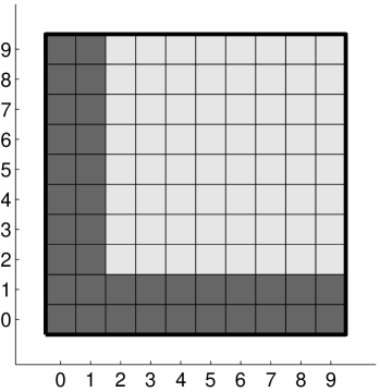
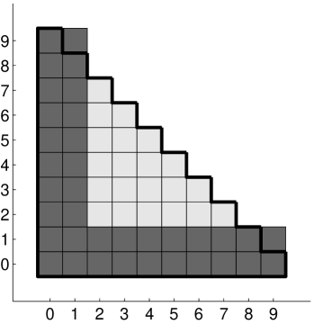
Figure 2.3: Full space $\mathcal{Q}_{p}(\hat{\tau})$ (left) and Serendipity space $\mathcal{Q}_{p}^{\oplus}(\hat{\tau})$ (right) for $p=9$.

gives a graphical representation of the two spaces. Therein a square at position $(i,j)$ stands for a basis function $\xi^{i}\eta^{j}$ of $\mathcal{Q}_{p}^{\clubsuit}(\hat{\tau})$. The darker squares correspond to those functions present in both spaces, while the lighter ones represent $\xi^{2}\eta^{2}\widetilde{\mathcal{Q}}(\hat{\tau})$. Note that it holds

$$\mathcal{P}_{p}\subset\mathcal{Q}_{p}^{\oplus}\subset\mathcal{Q}_{p}$$

and that $\mathcal{Q}_{p}^{\oplus}$ uses only about half the number of degrees of freedom that $\mathcal{Q}_{p}$ uses.

Now let us come to defining interpolation operators for these two spaces. We will consider two types of interpolation: vertex-edge-cell interpolation and Lagrange interpolation.

Vertex-edge-cell interpolation operator

The first interpolation operator is based on point evaluation at the vertices, line integrals along the edges and integrals over the cell interior, see [27, 38].

Let $\hat{a}_{i}$ and $\hat{e}_{i}$, $i=1,\ldots,4$, denote the vertices and edges of $\hat{\tau}$, respectively. We define the vertex-edge-cell interpolation operator $\hat{\pi}:C(\hat{\tau})\to\mathcal{Q}_{p}^{\clubsuit}(\hat{\tau})$ by

$$\hat{\pi}\hat{v}(\hat{a}_{i}) =\hat{v}(\hat{a}_{i}),\,\quad i=1,\dots,4,$$ (2.13a)

$$\int_{\hat{e}_{i}}(\hat{\pi}\hat{v})\hat{q} =\int_{\hat{e}_{i}}\hat{v}\hat{q},\quad i=1,\dots,4,\quad \hat{q}\in\mathcal{P}_{p-2}(\hat{e}_{i}),$$ (2.13b)

$$\iint_{\hat{\tau}}(\hat{\pi}\hat{v})\hat{q} =\iint_{\hat{\tau}}\hat{v}\hat{q}, \hat{q}\in\widetilde{\mathcal{Q}}(\hat{\tau}).$$ (2.13c)

This operator is uniquely defined and can be extended to the globally defined interpolation operator $\pi^{N}:C(\overline{\Omega})\to V^{N}$ by

$$(\pi^{N}v)|_{\tau}:=\big{(}\hat{\pi}(v\circ F_{\tau})\big{)}\circ F_{\tau}^{-1}\quad\forall\tau\in T^{N},\,v\in C(\overline{\Omega}),$$

with the bijective reference mapping $F_{\tau}:\hat{\tau}\to\tau$.

Lemma 2.5.

For the interpolation operator $\pi^{N}:C(\overline{\Omega})\rightarrow V^{N}$ the stability property

$$\left\|{\pi^{N}w}\right\|_{L_{\infty}(\tau)}\leq C\|{w}\|_{L_{\infty}(\tau)}\quad\forall w\in C(\tau),\,\forall\tau\subset\overline{\Omega},$$ (2.14)

holds and we have the anisotropic error estimates

$$\left\|{w-\pi^{N}w}\right\|_{L_{q}(\tau_{ij})} \leq C\sum_{r=0}^{s}\left\|{h_{i}^{s-r}k_{j}^{r}\frac{\partial^{s}w}{\partial x^{s-r}\partial y^{r}}}\right\|_{L_{q}(\tau_{ij})},$$ (2.15a)

$$\left\|{(w-\pi^{N}w)_{x}}\right\|_{L_{q}(\tau_{ij})} \leq C\sum_{r=0}^{t}\left\|{h_{i}^{t-r}k_{j}^{r}\frac{\partial^{t+1}w}{\partial x^{t-r+1}\partial y^{r}}}\right\|_{L_{q}(\tau_{ij})},$$ (2.15b)

$$\left\|{(w-\pi^{N}w)_{y}}\right\|_{L_{q}(\tau_{ij})} \leq C\sum_{r=0}^{t}\left\|{h_{i}^{t-r}k_{j}^{r}\frac{\partial^{t+1}w}{\partial x^{t-r}\partial y^{r+1}}}\right\|_{L_{q}(\tau_{ij})}$$ (2.15c)

for $\tau_{ij}\subset\overline{\Omega}$ and $q\in[1,\infty]$, $2\leq s\leq p+1$, $1\leq t\leq p$.

Proof.

The proof for arbitrary $\mathcal{Q}^{\clubsuit}_{p}$ can be found in [24] and for the full space $\mathcal{Q}_{p}$ also in e.g. [57]. ∎

Lagrange-type interpolation

The second interpolation type we consider is the Lagrange type, i.e. it uses only point-value information.

Let $-1=\xi_{0}<\xi_{1}<\dots<\xi_{p-1}<\xi_{p}=+1$ and $-1=\eta_{0}<\eta_{1}<\dots<\eta_{p-1}<\eta_{p}=+1$ be two increasing sequences of $p+1$ points of $[-1,+1]$ which include both end points. We define the Lagrange-type interpolation operator $\hat{J}:C(\hat{\tau})\to\mathcal{Q}_{p}^{\clubsuit}(\hat{\tau})$ by values at the vertices

$$\begin{aligned} (\hat{J}\hat{v})(\pm 1,-1)&:=\hat{v}(\pm 1,-1),&\qquad(\hat{J}\hat{v})(\pm 1,+1)&:=\hat{v}(\pm 1,+1)\end{aligned}$$ (2.16a)

values on the edges

$$\left.\begin{aligned} (\hat{J}\hat{v})(\xi_{i},\pm 1)&:=\hat{v}(\xi_{i},\pm 1),&\qquad&i=1,\dots,p-1,\\ (\hat{J}\hat{v})(\pm 1,\eta_{j})&:=\hat{v}(\pm 1,\eta_{j}),&\qquad&j=1,\dots,p-1,\\ \end{aligned}\qquad\right\}$$ (2.16b)

and values in the interior

$$\begin{aligned} (\hat{J}\hat{v})(\xi_{i+1},\eta_{j+1})&:=\hat{v}(\xi_{i+1},\eta_{j+1}),&\qquad&i=0,\dots,p-2,j=0,\dots,s_{i},\end{aligned}$$ (2.16c)

where the $s_{i}$ are those given in (2.12).

In [24] it is shown that this operator is uniquely defined. What is left to specify are the sequences $\{\xi_{i}\}$ and $\{\eta_{j}\}$. Here we consider two choices:

1) equidistant distribution: We define the operator $J^{N}:C(\overline{\Omega})\to V^{N}$ by

$$(J^{N}v)|_{\tau}:=\big{(}\hat{J}(v\circ F_{\tau})\big{)}\circ F_{\tau}^{-1}\quad\forall\tau\in T^{N},\,v\in C(\overline{\Omega}),$$

with the bijective reference mapping $F_{\tau}:\hat{\tau}\to\tau$ and the local sequences

$$\xi_{i}=\eta_{i}=-1+2i/p,\,i=0,\dots,p.$$

2) distribution according to the Gauß-Lobatto quadrature rule:
Let $-1=t_{0}<t_{1}<\dots<t_{p}=1$, be the zeros of

$$(1-t^{2})L_{p}^{\prime}(t)=0,\quad t\in[-1,1],$$

where $L_{p}$ is the Legendre polynomial of degree $p$. These points are also used in the Gauß-Lobatto quadrature rule of approximation order $2p-1$. Therefore, we refer to them as Gauß-Lobatto points. In literature they are also named Jacobi points [37] as they are also the zeros of the orthogonal Jacobi-polynomials $P_{p}^{(1,1)}$ of order $p$. Now we define the operator $I^{N}:C(\overline{\Omega})\to V^{N}$ by

$$(I^{N}v)|_{\tau}:=\big{(}\hat{J}(v\circ F_{\tau})\big{)}\circ F_{\tau}^{-1}\quad\forall\tau\in T^{N},\,v\in C(\overline{\Omega}),$$

with the bijective reference mapping $F_{\tau}:\hat{\tau}\to\tau$ and the local sequences

$$\xi_{i}=\eta_{i}=t_{i},\,i=0,\dots,p.$$

Lemma 2.6.

The interpolation operators $J^{N}:C(\overline{\Omega})\rightarrow V^{N}$ and $I^{N}:C(\overline{\Omega})\rightarrow V^{N}$ yield the stability property

$$\left\|{J^{N}w}\right\|_{L_{\infty}(\tau)}+\left\|{I^{N}w}\right\|_{L_{\infty}(\tau)}\leq C\|{w}\|_{L_{\infty}(\tau)}\quad\forall w\in C(\tau),\,\forall\tau\subset\overline{\Omega},$$ (2.17)

and we have the anisotropic error estimates

$$\left\|{w-J^{N}w}\right\|_{L_{q}(\tau_{ij})}+\left\|{w-I^{N}w}\right\|_{L_{q}(\tau_{ij})} \leq C\sum_{r=0}^{s}\left\|{h_{i}^{s-r}k_{j}^{r}\frac{\partial^{s}w}{\partial x^{s-r}\partial y^{r}}}\right\|_{L_{q}(\tau_{ij})},$$ (2.19a)

$$\left\|{(w-J^{N}w)_{x}}\right\|_{L_{q}(\tau_{ij})}+\left\|{(w-I^{N}w)_{x}}\right\|_{L_{q}(\tau_{ij})} \leq C\sum_{r=0}^{t}\left\|{h_{i}^{t-r}k_{j}^{r}\frac{\partial^{t+1}w}{\partial x^{t-r+1}\partial y^{r}}}\right\|_{L_{q}(\tau_{ij})},$$ (2.19b)

$$\left\|{(w-J^{N}w)_{y}}\right\|_{L_{q}(\tau_{ij})}+\left\|{(w-I^{N}w)_{y}}\right\|_{L_{q}(\tau_{ij})} \leq C\sum_{r=0}^{t}\left\|{h_{i}^{t-r}k_{j}^{r}\frac{\partial^{t+1}w}{\partial x^{t-r}\partial y^{r+1}}}\right\|_{L_{q}(\tau_{ij})}$$ (2.19c)

for $\tau_{ij}\subset\overline{\Omega}$ and $q\in[1,\infty]$, $2\leq s\leq p+1$, $1\leq t\leq p$.

Proof.

The proof for arbitrary $\mathcal{Q}^{\clubsuit}_{p}$ can be found in [24] and for the full space $\mathcal{Q}_{p}$ also in e.g. [1]. ∎

There is a strong connection between $\pi^{N}$ and $I^{N}$ in the case of $\mathcal{Q}_{p}$-elements. Let us spend a subscript for the polynomial order $p$, i.e. we write $\pi_{p}^{N}$ and $I_{p}^{N}$ for the interpolation operators mapping into $V^{N}$ with local polynomial spaces $\mathcal{Q}_{p}$. Then it holds the identity

$$\pi_{p}^{N}=I_{p}^{N}\pi_{p+1}^{N},$$ (2.20)

see [16, Lemma 3.3]. A direct consequence is the additional identity

$$\pi_{p}^{N}v=I_{p}^{N}v+(\pi^{N}_{p+1}v-v)+\left(I^{N}_{p}(\pi^{N}_{p+1}v-v)-(\pi^{N}_{p+1}v-v)\right)$$ (2.21)

for arbitrary $v\in C(\bar{\Omega})$. It shows the distance between both interpolation operators to be proportional to terms of order $p+1$. The identity (2.20) (with the properly redefinition of the interpolation operators therein) does also hold for the Serendipity spaces $\mathcal{Q}_{2}^{\oplus}$ and $\mathcal{Q}_{3}^{\oplus}$, but not for $\mathcal{Q}_{p}^{\oplus}$ with $p\geq 4$. This can be shown analogously to the proof of [16, Lemma 3.3].

The reason for the failed identity lies in the definition of the interior degrees of freedom (2.13c) and (2.16c). For $\mathcal{Q}_{2}^{\oplus}$ and $\mathcal{Q}_{3}^{\oplus}$ these conditions are not existent and therefore always fulfilled, while for higher order $p$ they do not match any more.

2.4 Numerical Methods

Let us come to the numerical methods that we will consider in the next chapter.

2.4.1 Galerkin FEM

The first method will be the unstabilised Galerkin FEM given by:

Find $u_{Gal}^{N}\in V^{N}$ such that

$$a_{Gal}(u_{Gal}^{N},v^{N})=(f,v^{N})\qquad\forall v^{N}\in V^{N}.$$ (2.22)

This problem possesses a unique solution due to (1.2). Furthermore, the Galerkin orthogonality

$$a_{Gal}(u-u_{Gal}^{N},v^{N})=0\qquad\forall v^{N}\in V^{N}$$ (2.23)

holds true and we have coercivity

$$a_{Gal}(v,v)\geq\left|\!\!\;\left|\!\!\;\left|{v}\right|\!\!\;\right|\!\!\;\right|_{\varepsilon}^{2},\qquad v\in H^{1}_{0}(\Omega)$$ (2.24)

where the energy norm is defined by (1.3)

$$\left|\!\!\;\left|\!\!\;\left|{v}\right|\!\!\;\right|\!\!\;\right|_{\varepsilon}:=\left(\varepsilon\|{\nabla v}\|_{0}^{2}+\gamma\|{v}\|_{0}^{2}\right)^{1/2}.$$

Since the standard Galerkin discretisation lacks stability even on S-type meshes, see the numerical results given in [43, 58], we will also consider stabilised methods. A survey of several different stabilised method for singularly perturbed problems can be found in the book [54].

2.4.2 Streamline Diffusion FEM

In 1979 Hughes and Brooks [29] introduced the streamline-diffusion finite element method (SDFEM), sometimes also called streamline upwind Petrov Galerkin finite element method (SUPG-FEM). This method provides highly accurate solutions outside the layers and good stability properties. Its basic idea is to add weighted local residuals to the variational formulation, i.e. to add

$$\delta_{\tau}(Lu-f,-bw_{x})_{\tau}=0$$

where the constant parameters $\delta_{\tau}=\delta_{ij}\geq 0$ for $\tau\subset\Omega_{ij}$ are user chosen and influence both stability and convergence. A slightly different approach will be used in Chapter 4.

Defining

$$a_{stabSD}(v,w):=\sum_{\tau\in T^{N}}\delta_{\tau}(\varepsilon\Delta v+bv_{x}-cv,bw_{x})_{\tau},\qquad\mbox{for all }v,\,w\in H^{1}_{0}(\Omega)$$

and

$$f_{SD}(w):=(f,w)-\sum_{\tau\in T^{N}}\delta_{\tau}(f,bw_{x})_{\tau},\quad\mbox{for all }w\in H_{0}^{1}(\Omega)$$

we obtain the streamline diffusion formulation of (1.1) by: Find $u_{SD}^{N}\in V^{N}$ such that

$$a_{SD}(u_{SD}^{N},v^{N}):=a_{Gal}(u_{SD}^{N},v^{N})+a_{stabSD}(u_{SD}^{N},v^{N})=f_{SD}(v^{N}),\quad\mbox{for all }v^{N}\in V^{N}.$$ (2.25)

Associated with this method is the streamline diffusion norm, defined by

$$\left|\!\!\;\left|\!\!\;\left|{v}\right|\!\!\;\right|\!\!\;\right|_{SD}:=\left(\varepsilon\|{\nabla v}\|_{0}^{2}+\gamma\|{v}\|_{0}^{2}+\sum_{\tau\in T^{N}}\delta_{\tau}\|{bv_{x}}\|_{0,\tau}^{2}\right)^{1/2}.$$ (2.26)

We have Galerkin orthogonality, and for

$$0\leq\delta_{\tau}\leq\frac{1}{2}\min\left\{\frac{\gamma}{\|{c}\|_{L_{\infty}(\tau)}^{2}},\frac{h_{\tau}^{2}}{\mu^{2}\varepsilon}\right\},$$ (2.27)

where $\mu\geq 0$ is a fixed constant such that the inverse inequality

$$\|{\Delta v^{N}}\|_{0,\tau}\leq\mu h_{\tau}^{-1}\|{\nabla v^{N}}\|_{0,\tau},\qquad\forall v^{N}\in V^{N},\,\tau\in T^{N}$$

holds with $h_{\tau_{ij}}:=\min\{h_{i},k_{j}\}$, we have coercivity

$$a_{SD}(v,v)\geq\frac{1}{2}\left|\!\!\;\left|\!\!\;\left|{v}\right|\!\!\;\right|\!\!\;\right|_{SD}^{2},\qquad v\in H^{1}_{0}(\Omega).$$ (2.28)

A disadvantage of the SDFEM are several additional terms including second order derivatives that have to be assembled in order to ensure the Galerkin orthogonality of the resulting method. Moreover, for systems of differential equations additional coupling between different species occurs.

2.4.3 Local Projection Stabilisation FEM

An alternative stabilisation technique overcoming some drawbacks of the SDFEM is the Local Projection Stabilisation method LPSFEM. Instead of adding weighted residuals, only weighted fluctuations $(id-\pi)$ of the streamline derivatives are added. Therein $\pi$ denotes a projection into a discontinuous finite element space.

Originally the method was introduced for Stokes and transport problems [5, 6], but also applied to the Oseen problem in [7, 46]. In its original definition, the local projection method was proposed as a two-level method, where the projection space is defined on a coarser mesh consisting of patches of elements [5, 6, 7]. In this case, standard finite element spaces can be used for both the approximation space and the projection space. Based on the existence of a special interpolation operator [46], the one level approach using enriched spaces was constructed. It was shown in [46] that it suffices to enrich the standard $\mathcal{Q}_{p}$-element, $p\geq 2$, in 2d by just two additional bubble functions of higher order. For its application on layer-adapted meshes for problems with exponential boundary layers see [45, 44].

Here we will use the one level approach without enriching the polynomial spaces. Let $\pi_{\tau}$ denote the $L_{2}$-projection into the finite dimensional function space $D(\tau)=\mathcal{P}_{p-2}(\tau)$. The fluctuation operator $\kappa_{\tau}:L_{2}(\tau)\to L_{2}(\tau)$ is defined by $\kappa_{\tau}v:=v-\pi_{\tau}v$. In order to get additional control on the derivative in streamline direction, we define the stabilisation term

$$s(u,v):=\sum_{\tau\in T^{N}}\delta_{\tau}\big{(}\kappa_{\tau}(bu_{x}),\kappa_{\tau}(bv_{x})\big{)}_{\tau}$$

with the parameters $\delta_{\tau}=\delta_{ij}\geq 0$, $\tau\subset\Omega_{ij}$, which will be specified later. It was stated in [12, 13] for different stabilisation methods that stabilisation is best if only applied in $\Omega_{11}\cup\Omega_{21}$. Therefore, we set $\delta_{12}=\delta_{22}=0$ in the following.

The stabilised bilinear form $a_{LPS}$ is defined by

$$a_{LPS}(u,v):=a_{Gal}(u,v)+s(u,v),\qquad u,v\in H^{1}_{0}(\Omega),$$

and the stabilised discrete problem reads:

Find $u_{LPS}^{N}\in V^{N}$ such that

$$a_{LPS}(u_{LPS}^{N},v^{N})=(f,v^{N})\qquad\forall v^{N}\in V^{N}.$$ (2.29)

Associated with this bilinear form is the LPS norm

$$\left|\!\!\;\left|\!\!\;\left|{v}\right|\!\!\;\right|\!\!\;\right|_{LPS}:=\left(\varepsilon\|{\nabla v}\|_{0}^{2}+\gamma\|{v}\|_{0}^{2}+s(v,v)\right)^{1/2}.$$ (2.30)

The bilinear form is coercive w.r.t. this norm

$$a_{LPS}(v,v)\geq\left|\!\!\;\left|\!\!\;\left|{v}\right|\!\!\;\right|\!\!\;\right|_{LPS}^{2},\qquad v\in H^{1}_{0}(\Omega).$$ (2.31)

Moreover, the solutions $u$ of (1.1) and $u_{LPS}^{N}$ of (2.29) do not fulfil the Galerkin orthogonality, but

$$a_{LPS}(u-u_{LPS}^{N},v^{N})=s(u,v^{N})\qquad\forall v^{N}\in V^{N}.$$ (2.32)

The LPSFEM gives control over the fluctuations of the streamline derivative. In [33] a slight variation of the formulation is considered and an inf-sup condition w.r.t. the SDFEM norm is shown on a quasi-regular mesh. Thus, this LPSFEM gives control over the full streamline derivative. Whether such a result holds on S-type meshes is not known.

Chapter 3 Uniform a-priori Error Estimation in Energy Norms

This chapter contains results from [23, 24, 14, 15] that are also given in Appendix Appendix, Appendix, Appendix and Appendix. All theoretical results will be accompanied by a numerical study using the singularly perturbed convection-diffusion problem

$$-\varepsilon\Delta u-(2-x)u_{x}+\frac{3}{2}u =f \text{in }\Omega=(0,1)^{2},$$ (3.1a)

$$u =0 \text{on }\partial\Omega,$$ (3.1b)

where the right-hand side $$f$$ is chosen such that

$$u(x,y)=\left(\cos\frac{\pi x}{2}-\frac{\mathrm{e}^{-x/\varepsilon}-\mathrm{e}^{-1/\varepsilon}}{1-\mathrm{e}^{-1/\varepsilon}}\right)\frac{\left(1-\mathrm{e}^{-y/\sqrt{\varepsilon}}\right)\left(1-\mathrm{e}^{-(1-y)/\sqrt{\varepsilon}}\right)}{1-\mathrm{e}^{-1/\sqrt{\varepsilon}}}$$ (3.1c)

is the solution. We will used a fixed perturbation parameter $\varepsilon=10^{-6}$. Computations verifying the uniformity w.r.t. $\varepsilon$ were also done. Figure 3.1

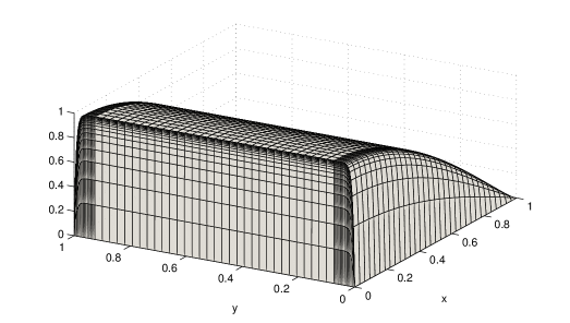
Figure 3.1: Typical solution of (1.1) with two parabolic layers and an exponential layer.

shows the resulting solution. For comparison, the energy norm of $u$ is in this case $\left|\!\!\;\left|\!\!\;\left|{u}\right|\!\!\;\right|\!\!\;\right|_{\varepsilon}\approx 0.9975$.

3.1 Results for Galerkin FEM

Let us start with results for the standard Galerkin FEM. In [21, 13] results for bilinear elements are presented. If the mesh parameter $\sigma$ fulfils $\sigma\geq 2$, then the convergence result of [51] holds

$$\left|\!\!\;\left|\!\!\;\left|{u-u_{Gal}^{N}}\right|\!\!\;\right|\!\!\;\right|_{\varepsilon}\leq C(N^{-1}\max|\psi^{\prime}|)$$

with $\max|\psi^{\prime}|$ from e.g. Table 2.1 and for $\sigma\geq 5/2$ the supercloseness result [21]

$$\left|\!\!\;\left|\!\!\;\left|{u^{I}-u_{Gal}^{N}}\right|\!\!\;\right|\!\!\;\right|_{\varepsilon}\leq C(N^{-1}\max|\psi^{\prime}|)^{2}$$

where $u^{I}$ denotes the nodal bilinear interpolant. In the higher-order case with either the full space $\mathcal{Q}_{p}$ or the serendipity space $\mathcal{Q}_{p}^{\oplus}$ results can be found in [24].

Theorem 3.1 (Theorem 6 of [24]).

Let the solution $u$ of (1.1) satisfy Assumption 2.1 and let $u_{Gal}^{N}$ denote the Galerkin solution of (2.22). Then, we have for $\sigma\geq p+1$

$$\left|\!\!\;\left|\!\!\;\left|{u-u_{Gal}^{N}}\right|\!\!\;\right|\!\!\;\right|_{\varepsilon}\leq C\big{(}N^{-1}\max|\psi^{\prime}|\big{)}^{p}.$$ (3.2)

Thus, similar to the bilinear case, we achieve convergence of order $p$ in the energy norm. To our knowledge, no supercloseness result is available in literature in the higher-order case. Nevertheless, it can be observed numerically for the full space $\mathcal{Q}_{p}$.

Let us come to the numerical example  (3.1). We will use a Bakhvalov-S-mesh, as here $|\max\psi^{\prime}|$ is bounded by a constant, see Table 2.1, and the convergence rates can be observed easiest. According to Theorem 3.1 we expect

$$\left|\!\!\;\left|\!\!\;\left|{u-u_{Gal}^{N}}\right|\!\!\;\right|\!\!\;\right|_{\varepsilon}\leq CN^{-p}.$$

Table 3.1

Table 3.1: Convergence errors of Galerkin FEM for $\mathcal{Q}_{p}$- and $\mathcal{Q}_{p}^{\oplus}$-elements, and $p=4,\,5$

	$\left|\!\!\;\left|\!\!\;\left|{u-u_{Gal}^{N}}\right|\!\!\;\right|\!\!\;\right|_{\varepsilon}$
$N$	$\mathcal{Q}_{4}$		$\mathcal{Q}_{4}^{\oplus}$		$\mathcal{Q}_{5}$		$\mathcal{Q}_{5}^{\oplus}$
8	6.633e-04	3.65	1.469e-03	3.68	1.330e-04	4.59	5.002e-04	4.53
16	5.274e-05	3.83	1.147e-04	3.87	5.506e-06	4.79	2.160e-05	4.81
32	3.715e-06	3.91	7.857e-06	3.94	1.985e-07	4.89	7.722e-07	4.92
64	2.467e-07	3.96	5.106e-07	3.97	6.682e-09	4.95	2.553e-08	4.94
128	1.590e-08	3.98	3.248e-08	3.99	2.169e-10	4.72	8.319e-10	0.12
256	1.009e-09	3.98	2.046e-09	3.99	8.216e-12		7.644e-10
320	4.148e-10		8.396e-10

confirms our expectation. In this table the errors and their estimated orders of convergence are given for $\sigma=p+3/2$. We see for the spaces $\mathcal{Q}_{4}$ and $\mathcal{Q}_{4}^{\oplus}$ a convergence of order four, while for the spaces $\mathcal{Q}_{5}$ and $\mathcal{Q}_{5}^{\oplus}$ we obtain order five. Moreover, the switch from the full space to Serendipity-space does increase the error only by a factor of two for $p=4$ and four for $p=5$. Thus the error is increased, but at the same time only about half the number of degrees of freedom are used.

Let us also look at supercloseness. Although no analytical result is given, Table 3.2

Table 3.2: Supercloseness property of Galerkin FEM for $p=5$

	$\mathcal{Q}_{5}$						$\mathcal{Q}_{5}^{\oplus}$
$N$	$\left|\!\!\;\left|\!\!\;\left|{\pi^{N}u-u_{Gal}^{N}}\right|\!\!\;\right|\!\!\;\right|_{\varepsilon}$		$\left|\!\!\;\left|\!\!\;\left|{I^{N}u-u_{Gal}^{N}}\right|\!\!\;\right|\!\!\;\right|_{\varepsilon}$		$\left|\!\!\;\left|\!\!\;\left|{J^{N}u-u_{Gal}^{N}}\right|\!\!\;\right|\!\!\;\right|_{\varepsilon}$		$\left|\!\!\;\left|\!\!\;\left|{\pi^{N}u-u_{Gal}^{N}}\right|\!\!\;\right|\!\!\;\right|_{\varepsilon}$
8	3.026e-05	5.48	3.408e-05	5.41	9.474e-05	4.60	2.825e-04	4.37
16	6.765e-07	5.80	8.003e-07	5.74	3.894e-06	4.79	1.366e-05	4.68
32	1.213e-08	5.92	1.496e-08	5.88	1.406e-07	4.89	5.314e-07	4.83
64	1.999e-10	5.87	2.537e-10	5.88	4.736e-09	4.94	1.871e-08	4.86
128	3.428e-12	-0.38	4.320e-12	-0.04	1.538e-10	4.55	6.423e-10	-0.25
256	4.461e-12		4.442e-12		6.580e-12		7.642e-10

shows for $p=5$ a supercloseness property of order $p+1$ for the Galerkin FEM with $\mathcal{Q}_{p}$-elements and the two interpolation operators $\pi^{N}$ (vertex-edge-cell interpolation) and $I^{N}$ (Gauß-Lobatto interpolation). No such property is evident for $J^{N}$ (equidistant Lagrange interpolation) or the Serendipity-elements.

For other polynomial degrees similar tables and conclusions can be given and are therefore omitted. We come back to the behaviour of $\pi^{N}$ and $I^{N}$ in the next section.

3.2 Results for SDFEM

One of the most popular stabilisation methods is the SDFEM. This method can also be used in connection with the general higher-order elements. Under certain restrictions on the stabilisation parameters convergence of order $p$ can be proved.

Theorem 3.2 (Theorem 8 of [14]).

Let

$$\delta_{11}\leq C,\quad\delta_{21}\leq C\max\{1,\varepsilon^{-1/2}(N^{-1}\max|\psi^{\prime}|)^{2/3}\}(N^{-1}\max|\psi^{\prime}|)^{4/3},\quad\delta_{12}=\delta_{22}=0,$$

and (2.27) be satisfied. Let $u$ be the solution of (1.1) fulfilling Assumption 2.1 and $u^{N}_{SD}$ be the streamline diffusion solution of (2.25). Then it holds for $\sigma\geq p+1$ that

$$\left|\!\!\;\left|\!\!\;\left|{u-u^{N}_{SD}}\right|\!\!\;\right|\!\!\;\right|_{\varepsilon}\leq C(N^{-1}\max|\psi^{\prime}|)^{p}.$$

Proof.

For the standard Shishkin mesh the proof is given in [14, Theorem 8] based mainly on Lemma 6 therein. For the Bakhvalov S-mesh the result is stated in [15]. The proof for a general S-type mesh can be done in a very similar way to [14] and one obtains

$$a_{stabSD}(u-\pi^{N}u,\chi)\leq C\big{[}\delta_{11}^{1/2} N^{-p}+\delta_{12}\varepsilon^{-1}(N^{-1}\max|\psi^{\prime}|)^{p-1}$$ (3.3)

$$+ \min\{\delta_{21}^{1/2}\varepsilon^{1/4},\delta_{21}^{3/4}\}(N^{-1}\max|\psi^{\prime}|)^{p-1}$$

$$+ \min\{\delta_{22}\varepsilon^{-3/4},\delta_{22}^{1/2}\varepsilon^{-1/4}\}(\ln N)^{1/2}(N^{-1}\max|\psi^{\prime}|)^{p-1}\big{]}\left|\!\!\;\left|\!\!\;\left|{\chi}\right|\!\!\;\right|\!\!\;\right|_{SD}$$

which together with the result for the Galerkin bilinear form [23, Theorem 13], coercivity (2.28) and the interpolation error [23, Theorem 12] gives above theorem. ∎

It can be seen quite nicely, that $|a_{stabSD}(u-\pi^{N}u,\chi)|$ becomes smaller, if the stabilisation parameters are reduced. But there is also an interaction between the Galerkin bilinear form $a_{Gal}(u-\pi^{N}u,\chi)$ and the SDFEM norm, that can be exploited to prove supercloseness. In order to do so, we will need an extension of Assumption 2.1 on the solution decomposition.

Assumption 3.3.

Let the solution $u$ of (1.1) be decomposable according to Assumption 2.1 into

$$u=v+w_{1}+w_{2}+w_{12}.$$

In addition to the pointwise bounds for $i+j\leq p+1$ stated in Assumption 2.1 we assume the $L_{2}$-norm bounds

$$\left\|{\frac{\partial^{p+2}v}{\partial x^{i}\partial y^{j}}}\right\|_{0} \leq C, \left\|{\frac{\partial^{p+2}w_{1}}{\partial x^{i}\partial y^{j}}}\right\|_{0} \leq C\varepsilon^{-i+1/2},$$

$$\left\|{\frac{\partial^{p+2}w_{2}}{\partial x^{i}\partial y^{j}}}\right\|_{0} \leq C\varepsilon^{-j/2+1/4}, \left\|{\frac{\partial^{p+2}w_{12}}{\partial x^{i}\partial y^{j}}}\right\|_{0} \leq C\varepsilon^{-i-j/2+3/4}$$

for $i+j=p+2$ with either $i=1$ or $j=1$.

Having this additional smoothness, the integral identities by Lin, see [57, 38, 62] can be used. Here we cite [57, Lemma 4].

Lemma 3.4.

Let $w\in H^{p+2}(\tau_{ij})$. Then for each $\chi\in\mathcal{Q}_{p}(\tau_{ij})$ we have

$$\left|\left((\pi^{N}w-w)_{x},\chi_{x}\right)_{\tau_{ij}}\right| \leq C\left\|{k_{j}^{p+1}\frac{\partial^{p+2}w}{\partial x\partial y^{p+1}}}\right\|_{0,\tau_{ij}}\|{\chi_{x}}\|_{0,\tau_{ij}}$$

$$\mbox{and}\hskip 28.45274pt\left|\left((\pi^{N}w-w)_{y},\chi_{y}\right)_{\tau_{ij}}\right| \leq C\left\|{h_{i}^{p+1}\frac{\partial^{p+2}w}{\partial x^{p+1}\partial y}}\right\|_{0,\tau_{ij}}\|{\chi_{y}}\|_{0,\tau_{ij}}.\hskip 42.67912pt\leavevmode\nobreak\$$

A different approach was used in [9, 10]. Therein a method attributed to Zlámal [63] is applied by adding and subtracting a certain higher-order polynomial and using its approximation properties. Although only done for bilinear finite elements, it seems plausible that a similar technique might work in the higher-order case.

Note that identities like those given in Lemma 3.4 do not hold for proper subspaces $\mathcal{Q}_{p}^{\clubsuit}\subset\mathcal{Q}_{p}$. Therefore, they cannot be used to prove a supercloseness property for spaces like the Serendipity space. This is not a real drawback, as for proper subspaces no supercloseness property is observed numerically.

Under above assumptions, [14] gives a supercloseness result for the SDFEM method.

Theorem 3.5 (Theorem 13 of [14]).

For $\mathcal{Q}_{p}^{\clubsuit}=\mathcal{Q}_{p}$, $\sigma\geq p+1$

$$\delta_{11}=CN^{-1},\quad\delta_{21}\leq C\max\{1,\varepsilon^{-1/2}(N^{-1}\max|\psi^{\prime}|)\}(N^{-1}\max|\psi^{\prime}|)^{2},\quad\delta_{12}=\delta_{22}=0$$

and (2.27) we have

$$\left|\!\!\;\left|\!\!\;\left|{\pi^{N}u-u^{N}_{SD}}\right|\!\!\;\right|\!\!\;\right|_{SD}\leq C(N^{-1}\max|\psi^{\prime}|)^{p+1/2}(\max|\psi^{\prime}|\ln N)^{1/2}.$$

Proof.

In [14] the proof for the standard Shishkin mesh can be found. The adaptation to general S-type meshes is straight-forward. The proof itself is based on the idea to estimate parts of the convective term of $a_{Gal}(\cdot,\cdot)$ by the SDFEM norm instead of the energy norm, see [57]. To be more precise, it’s main step is

$$|(\pi^{N}u-u,b\chi_{x})_{\Omega_{11}}| \leq C\|{\pi^{N}u-u}\|_{0,\Omega_{11}}\|{b\chi_{x}}\|_{0,\Omega_{11}}$$

$$\leq CN^{-(p+1)}\|{b\chi_{x}}\|_{0,\Omega_{11}}$$

$$\leq C\min\{\varepsilon^{-1/2},\delta_{11}^{-1/2}\}N^{-(p+1)}\left|\!\!\;\left|\!\!\;\left|{\chi}\right|\!\!\;\right|\!\!\;\right|_{SD}$$

that leads to

$$|((\pi^{N}u-u),b\chi_{x})|\leq C\bigg{(}\min\{\varepsilon^{-1/2},\delta_{11}^{-1/2}\}N^{-(p+1)}+\\ (1+\min\{\delta_{21}^{-1/4},N^{1/2}\})(N^{-1}\max|\psi^{\prime}|)^{p+1}(\ln N)^{1/2}\bigg{)}\left|\!\!\;\left|\!\!\;\left|{\chi}\right|\!\!\;\right|\!\!\;\right|_{SD}.$$ (3.4)

The new bounds on the stabilisation parameters are consequences of (3.3). ∎

Remark 3.6.

In order to achieve the supercloseness property we have to stabilise in $\Omega_{11}$. In the characteristic layer region we may stabilise, but this is not necessary for supercloseness. By choosing $\delta_{21}=C(N^{-1}\max|\psi^{\prime}|)^{2}$ above result can be slightly improved to

$$\left|\!\!\;\left|\!\!\;\left|{\pi^{N}u-u^{N}_{SD}}\right|\!\!\;\right|\!\!\;\right|_{SD}\leq C(N^{-1}\max|\psi^{\prime}|)^{p+1/2}(\ln N)^{1/2}.$$

The bound (3.4) does also show, that for $\varepsilon\geq N^{-1}$ even the Galerkin FEM ($\delta_{11}=\delta_{21}=0$) fulfils a supercloseness property of order $p+1/2$. Unfortunately, this case is of little interest in general.

We have already seen in Section 3.1 that the two interpolation operators $\pi^{N}$ (vertex-edge-cell interpolation) and $I^{N}$ (Gauß-Lobatto interpolation) show a similar numerical behaviour. Recalling (2.21)

$$\pi_{p}^{N}v=I_{p}^{N}v+(\pi^{N}_{p+1}v-v)+\left(I^{N}_{p}(\pi^{N}_{p+1}v-v)-(\pi^{N}_{p+1}v-v)\right)$$

we obtain

$$\left|\!\!\;\left|\!\!\;\left|{I_{p}^{N}u-u_{SD}^{N}}\right|\!\!\;\right|\!\!\;\right|_{\varepsilon}\leq\left|\!\!\;\left|\!\!\;\left|{\pi_{p}^{N}u-u^{N}_{SD}}\right|\!\!\;\right|\!\!\;\right|_{\varepsilon}+\left|\!\!\;\left|\!\!\;\left|{I_{p}^{N}(\pi_{p+1}^{N}u-u)-(\pi_{p+1}^{N}u-u)}\right|\!\!\;\right|\!\!\;\right|_{\varepsilon}+\left|\!\!\;\left|\!\!\;\left|{\pi_{p+1}^{N}u-u}\right|\!\!\;\right|\!\!\;\right|_{\varepsilon}.$$

Now the first term is estimated in Theorem 3.5, while the other two terms are interpolation errors of higher-order. Combining the results gives [16, Theorem 4.8].

Theorem 3.7 (Theorem 4.8 of [16]).

Let $\sigma\geq p+2$. Then it holds for the streamline-diffusion solution $u^{N}_{SD}$ under the restrictions on the stabilisation parameters given in Theorem 3.5

$$\left|\!\!\;\left|\!\!\;\left|{I^{N}u-u^{N}_{SD}}\right|\!\!\;\right|\!\!\;\right|_{\varepsilon}\leq C(N^{-1}\max|\psi^{\prime}|)^{p+1/2}(\max|\psi^{\prime}|\ln N)^{1/2}.$$

Thus, the Gauß-Lobatto interpolation inherits the supercloseness property from the vertex-edge-cell interpolation. A supercloseness property can be used to enhance the quality of the solution by a simple postprocessing routine.

Figure 3.2: Macroelements $M$ of $\tilde{T}^{N/2}$ constructed from $T^{N}$

Suppose $N$ is divisible by 8. We construct a coarser macro mesh $\tilde{T}^{N/2}$ composed of macro rectangles $M$, each consisting of four rectangles of $T^{N}$. The construction of these macro elements $M$ is done such that the union of them covers $\Omega$ and none of them crosses the transition lines at $x=\lambda_{x}$ and at $y=\lambda_{y}$ or $y=1-\lambda_{y}$, see Figure 3.2. Remark that in general $\tilde{T}^{N/2}\neq T^{N/2}$ due to different transition points $\lambda_{x}$ and $\lambda_{y}$, and the mesh generating function $\phi$.

We now define local postprocessing operators for one macro element $M\in\tilde{T}^{N/2}$. The precise definition can be found in [16], we will give only the basic ideas here.

The first one was presented in 1d in [60] and is a modification of an operator given in [38]. Let the local operator $\widehat{P}_{vec}:C[-1,1]\to\mathcal{P}_{p+1}[-1,1]$ be given on the reference interval $[-1,1]$ by

$$\widehat{P}_{vec}\hat{v}(-1) =v(x_{i-1}),\qquad\widehat{P}_{vec}\hat{v}(a)=v(x_{i}),\qquad\widehat{P}_{vec}\hat{v}(1)=v(x_{i+1}),$$

$$\mbox{and for $p=2$:}\hskip 28.45274pt\int_{-1}^{1}(\widehat{P}_{vec}\hat{v}-\hat{v}) =0,$$

$$\mbox{while for $p\geq 3$:}\hskip 28.45274pt\int_{-1}^{a}(\widehat{P}_{vec}\hat{v}-\hat{v}) =0,\quad\int_{a}^{1}(\widehat{P}_{vec}\hat{v}-\hat{v})=0,$$

$$\int_{-1}^{1}(\widehat{P}_{vec}\hat{v}-\hat{v})q =0,\quad q\in\mathcal{P}_{p-2}[-1,1]\setminus\mathbb{R},$$

where $\hat{v}$ is a function $v|_{[x_{i-1},x_{i+1}]}$ linearly mapped onto the reference interval and $a\in(-1,1)$ is the point that $x_{i}$ is mapped onto. By using the reference mapping and the tensor product structure, we obtain the full postprocessing operator $P_{vec,M}:C(M)\to\mathcal{Q}_{p+1}(M)$ on each macro element. Then, this piecewise projection is extended to a global, continuous operator $P_{vec}$.

The second postprocessing operator is defined by using the ordered sample of Gauß-Lobatto points $\{(\tilde{x}_{i},\tilde{y}_{j})\}$, $i,j=0,\dots,2p$ of the four rectangles that $M$ consists of.

Let $P_{GL,M}:C(M)\to\mathcal{Q}_{p+1}(M)$ denote the projection/interpolation operator fulfilling

$$P_{GL,M}v(\tilde{x}_{i},\tilde{y}_{j})=v(\tilde{x}_{i},\tilde{y}_{j}),\quad i,j=0,\,1,\,3,\,5,\dots,2p-3,2p-1,\,2p.$$

Then, this piecewise projection is extended to a global, continuous operator $P_{GL}$.

We have for the postprocessed numerical solutions the following superconvergence result [16, Theorem 5.2].

Theorem 3.8 (Theorem 5.2 of [16]).

Let $\sigma\geq p+2$. Then it holds for the streamline-diffusion solution $u^{N}_{SD}$ under the restrictions on the stabilisation parameters given in Theorem 3.5

$$\left|\!\!\;\left|\!\!\;\left|{u-P_{GL}u^{N}_{SD}}\right|\!\!\;\right|\!\!\;\right|_{\varepsilon}+\left|\!\!\;\left|\!\!\;\left|{u-P_{vec}u^{N}_{SD}}\right|\!\!\;\right|\!\!\;\right|_{\varepsilon}\leq C(N^{-1}\max|\psi^{\prime}|)^{p+1/2}(\max|\psi^{\prime}|\ln N)^{1/2}.$$

Let us come to the numerical example  (3.1). Although Theorems 3.7 and 3.8 assume $\sigma\geq p+2$ we will use a Bakhvalov-S-mesh with $\sigma=p+3/2$ and $\varepsilon=10^{-6}$ as numerical results suggest this to be enough. Note also, that in the bilinear case $\sigma=1+3/2$ is a standard choice for superconvergence simulations, [62, 22, 21]. For the stabilisation parameters we have two choices, according to Theorems 3.2 and 3.5:

$$\delta_{11} =C_{SD},\quad\delta_{21}=C_{SD}\varepsilon^{-1/2}N^{-2},\quad\delta_{12}=\delta_{22}=0,$$ (3.5a)

$$\mbox{or}\qquad\delta_{11} =C_{SD}N^{-1},\quad\delta_{21}=C_{SD}\varepsilon^{-1/2}N^{-3},\quad\delta_{12}=\delta_{22}=0.$$ (3.5b)

For both our investigations into convergence and superconvergence we will use the smaller parameters, i.e. (3.5b). The influence of $C_{SD}$ to various norms can be seen in Figure 3.3 using $N=64$ and $\varepsilon=10^{-6}$.

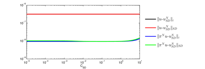
Figure 3.3: Influence of the stabilisation constant $C_{SD}$ onto the error behaviour

Therein, the norms are not strongly influenced by the choice of moderate values of $C_{SD}$. Thus, in the following we will use $C_{SD}=1$.

Table 3.3

Table 3.3: Convergence errors of SDFEM for $\mathcal{Q}_{p}$- and $\mathcal{Q}_{p}^{\oplus}$-elements, and $p=4,\,5$ with $\delta_{ij}$ according to (3.5b)

	$\left|\!\!\;\left|\!\!\;\left|{u-u_{SD}^{N}}\right|\!\!\;\right|\!\!\;\right|_{\varepsilon}$
$N$	$\mathcal{Q}_{4}$		$\mathcal{Q}_{4}^{\oplus}$		$\mathcal{Q}_{5}$		$\mathcal{Q}_{5}^{\oplus}$
8	6.709e-04	3.66	1.480e-03	3.69	2.198e-04	4.67	5.331e-04	4.56
16	5.308e-05	3.84	1.150e-04	3.87	8.634e-06	5.34	2.258e-05	4.86
32	3.715e-06	3.91	7.859e-06	3.94	2.134e-07	4.99	7.761e-07	4.93
64	2.467e-07	3.96	5.107e-07	3.97	6.722e-09	4.95	2.554e-08	4.94
128	1.590e-08	3.98	3.248e-08	3.99	2.170e-10	4.59	8.330e-10	0.14
256	1.009e-09	3.99	2.046e-09	3.99	8.989e-12		7.585e-10
320	4.147e-10		8.396e-10

shows the results for the polynomial spaces $\mathcal{Q}_{p}$ and $\mathcal{Q}_{p}^{\oplus}$ in the cases $p=4$ and $p=5$. As we can see, the convergence orders of $p$ are achieved and again we only have a constant factor of about 2 ($p=4$) and about 3 ($p=5$) in the errors when switching from the full to the Serendipity space.

Table 3.4: Supercloseness property of SDFEM for $p=4$ and $\delta_{ij}$ according to (3.5b)

	$\mathcal{Q}_{4}$						$\mathcal{Q}_{4}^{\oplus}$
$N$	$\left|\!\!\;\left|\!\!\;\left|{\pi^{N}u-u_{SD}^{N}}\right|\!\!\;\right|\!\!\;\right|_{\varepsilon}$		$\left|\!\!\;\left|\!\!\;\left|{I^{N}u-u_{SD}^{N}}\right|\!\!\;\right|\!\!\;\right|_{\varepsilon}$		$\left|\!\!\;\left|\!\!\;\left|{J^{N}u-u_{SD}^{N}}\right|\!\!\;\right|\!\!\;\right|_{\varepsilon}$		$\left|\!\!\;\left|\!\!\;\left|{\pi^{N}u-u_{SD}^{N}}\right|\!\!\;\right|\!\!\;\right|_{\varepsilon}$
8	1.717e-04	4.28	2.004e-04	4.31	3.241e-04	3.78	6.824e-04	3.46
16	8.810e-06	5.10	1.009e-05	5.00	2.358e-05	3.91	6.204e-05	3.69
32	2.566e-07	4.95	3.150e-07	4.92	1.572e-06	3.92	4.798e-06	3.83
64	8.302e-09	4.95	1.041e-08	4.94	1.036e-07	3.96	3.375e-07	3.91
128	2.679e-10	4.91	3.385e-10	4.89	6.669e-09	3.98	2.242e-08	3.96
256	8.919e-12	1.38	1.144e-11	2.14	4.232e-10	3.98	1.445e-09	3.97
320	6.550e-12		7.098e-12		1.740e-10		5.959e-10

As predicted by Theorems 3.5 and 3.7 we observe in Table 3.4 for the case $p=4$ a supercloseness property. But, the order is $p+1$ for both the vertex-edge-cell interpolation operator $\pi^{N}$ and the Gauß-Lobatto interpolation operator $I^{N}$ instead of the predicted $p+1/2$. Thus the analytical results may not be sharp. Note that for the equidistant-interpolation operator $J^{N}$ and for the Serendipity space this property is not evident.

Let us now come to exploiting the supercloseness property. Table 3.5

Table 3.5: Postprocessing of SDFEM for $\mathcal{Q}_{4}$ and $\delta_{ij}$ according to (3.5b)

$N$	$\left|\!\!\;\left|\!\!\;\left|{u-P_{vec}u_{SD}^{N}}\right|\!\!\;\right|\!\!\;\right|_{\varepsilon}$		$\left|\!\!\;\left|\!\!\;\left|{u-P_{GL}u_{SD}^{N}}\right|\!\!\;\right|\!\!\;\right|_{\varepsilon}$
8	4.725e-03	4.68	1.196e-02	4.80
16	1.850e-04	4.92	4.301e-04	5.15
32	6.104e-06	4.99	1.210e-05	5.27
64	1.918e-07	5.01	3.145e-07	5.28
128	5.961e-09	5.01	8.091e-09	5.24
256	1.853e-10	5.00	2.143e-10	5.15
320	6.071e-11		6.794e-11

gives the results of applying the postprocessing operators $P_{vec}$ and $P_{GL}$ to the SDFEM-solution. In correspondence with Theorem 3.8 we observe an improved convergence behaviour. We see a superconvergence of order $p+1$, half an order better than predicted.

Note that simulations with other polynomial degrees show similar results.

3.3 Results for LPSFEM

Finally, we analyse the LPSFEM. For its application to (1.1) with general higher-order elements we find a convergence result of order $p$ in [24].

Theorem 3.9 (Theorem 6 of [24]).

Let the solution $u$ of (1.1) satisfy Assumption 2.1. If the stabilisation parameters are chosen according to

$$\delta_{11}\leq C_{LPS}N^{-2}\big{(}\max|\psi^{\prime}|\big{)}^{2p},\,\delta_{21}\leq C_{LPS}\varepsilon^{-1/2}\ln^{-1}N\big{(}N^{-1}\max|\psi^{\prime}|\big{)}^{2},\,\delta_{12}=\delta_{22}=0$$ (3.6)

where $C_{LPS}>0$ is a constant and $\sigma\geq p+1$, we have for the LPSFEM solution $u_{LPS}^{N}$ of (2.29)

$$\left|\!\!\;\left|\!\!\;\left|{u-u_{LPS}^{N}}\right|\!\!\;\right|\!\!\;\right|_{\varepsilon}\leq C\big{(}N^{-1}\max|\psi^{\prime}|\big{)}^{p}.$$ (3.7)

Thus, if the stabilisation parameters are not too large then the convergence order $p$ of the Galerkin FEM is not disturbed. Similarly to the Galerkin FEM, no supercloseness result is known in the higher-order case. A supercloseness property of order two was shown for bilinear elements in [23].

When analysing the SDFEM we proved superconvergence by bounding the convective term of the Galerkin bilinear form against terms in the SDFEM norm. Unfortunately this trick does not help here with the LPSFEM. Basically, there are two problems. First, the convective term cannot easily be bounded by the stabilisation term, as the stabilisation terms only include fluctuations of the convection. Here the idea of [33] may help and we may use a stronger LPS-SDFEM norm, where the full weighted streamline derivative is included. But then the second problem comes into play. In order to estimate with the streamline derivative part of the norm we have to borrow half an order of the stabilisation parameter $\delta_{11}$, cf. (3.4). This costs us $\delta_{11}^{-1/2}\geq N/(\max|\psi^{\prime}|)^{p}$ by (3.6). Thus there would be no benefit in estimating with the stronger LPS norm.

Let us now look at the numerical example  (3.1). Again we will use a Bakhvalov-S-mesh with $\sigma=p+3/2$ and $\varepsilon=10^{-6}$. The stabilisation parameters are chosen according to Theorem 3.9. The influence of $C_{LPS}$ to various norms can be seen in Figure 3.4 using $N=64$ and $\varepsilon=10^{-6}$.

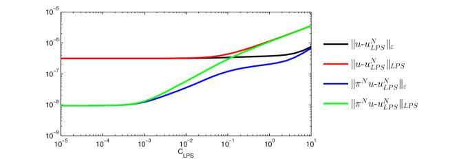
Figure 3.4: Influence of the stabilisation constant $C_{LPS}$ onto the error behaviour

Clearly, for larger values of $C_{LPS}$ more stabilisation is introduced. On the downside, if $C_{LPS}$ is too large the stabilisation term dominates the weak formulation of (1.1) unless $N$ is large enough. Therefore we have chosen for the following simulations $C_{LPS}=0.001$, i.e.

$$\delta_{11}\leq 0.001N^{-2}\big{(}\max|\psi^{\prime}|\big{)}^{2p},\,\delta_{21}\leq 0.001\varepsilon^{-1/2}\ln^{-1}N\big{(}N^{-1}\max|\psi^{\prime}|\big{)}^{2},\,\delta_{12}=\delta_{22}=0.$$ (3.8)

Table 3.6

Table 3.6: Convergence errors of LPSFEM for $\mathcal{Q}_{p}$- and $\mathcal{Q}_{p}^{\oplus}$-elements, and $p=4,\,5$ with $\delta_{ij}$ according to (3.8)

	$\left|\!\!\;\left|\!\!\;\left|{u-u_{LPS}^{N}}\right|\!\!\;\right|\!\!\;\right|_{\varepsilon}$
$N$	$\mathcal{Q}_{4}$		$\mathcal{Q}_{4}^{\oplus}$		$\mathcal{Q}_{5}$		$\mathcal{Q}_{5}^{\oplus}$
8	8.348e-04	3.64	1.892e-03	3.64	1.088e-04	4.61	3.715e-04	4.57
16	6.716e-05	3.82	1.518e-04	3.86	4.457e-06	4.81	1.560e-05	4.82
32	4.752e-06	3.91	1.046e-05	3.94	1.584e-07	4.90	5.532e-07	4.92
64	3.160e-07	3.96	6.796e-07	3.98	5.291e-09	4.95	1.828e-08	4.94
128	2.037e-08	3.98	4.316e-08	3.99	1.713e-10	4.42	5.970e-10	-0.29
256	1.293e-09	3.99	2.716e-09	3.99	8.005e-12		7.319e-10
320	5.313e-10		1.114e-09

shows the convergence behaviour of the LPSFEM for the same polynomial spaces as Table 3.3. Again we see convergence of order $p$ for the full and the Serendipity spaces. Although the Serendipity spaces need only half the number of degrees of freedom, and are therefore much cheaper in computation, only a factor of 2-4 lies between the errors of the full space and those of the Serendipity space.

Numerically, the LPSFEM does possess a supercloseness property too. Table 3.7

Table 3.7: Supercloseness property of LPSFEM for $p=4$ and $\delta_{ij}$ according to (3.8)

	$\mathcal{Q}_{4}$						$\mathcal{Q}_{4}^{\oplus}$
$N$	$\left|\!\!\;\left|\!\!\;\left|{\pi^{N}u-u_{LPS}^{N}}\right|\!\!\;\right|\!\!\;\right|_{\varepsilon}$		$\left|\!\!\;\left|\!\!\;\left|{I^{N}u-u_{LPS}^{N}}\right|\!\!\;\right|\!\!\;\right|_{\varepsilon}$		$\left|\!\!\;\left|\!\!\;\left|{J^{N}u-u_{LPS}^{N}}\right|\!\!\;\right|\!\!\;\right|_{\varepsilon}$		$\left|\!\!\;\left|\!\!\;\left|{\pi^{N}u-u_{LPS}^{N}}\right|\!\!\;\right|\!\!\;\right|_{\varepsilon}$
8	1.794e-04	4.50	2.167e-04	4.48	3.868e-04	3.74	8.717e-04	3.42
16	7.909e-06	4.66	9.740e-06	4.68	2.885e-05	3.85	8.156e-05	3.67
32	3.127e-07	4.68	3.790e-07	4.74	2.007e-06	3.92	6.395e-06	3.82
64	1.216e-08	4.84	1.419e-08	4.86	1.328e-07	3.96	4.524e-07	3.91
128	4.248e-10	4.99	4.871e-10	4.96	8.547e-09	3.98	3.017e-08	3.95
256	1.339e-11	3.27	1.566e-11	3.52	5.422e-10	3.99	1.949e-09	3.97
320	6.456e-12		7.133e-12		2.228e-10		8.039e-10

shows it for the standard choice of the stabilisation parameters (3.8). Here for $p=4$ the vertex-edge-cell interpolation operator $\pi^{N}$ and the Gauß-Lobatto interpolation operator $I^{N}$ show for the full space $\mathcal{Q}_{p}$ a supercloseness property of order $p+1$. So far, there is no theoretical explanation known for this fact. Similarly to the SDFEM and the Galerkin method, the equidistant interpolation operator $J^{N}$ and the Serendipity space do not possess such a property.

Chapter 4 What is the right norm?

This chapter contains results from [25] that are also given in Appendix Appendix. Here we consider only bilinear elements, i.e.

$$V^{N}:=\Big{\{}v\in H_{0}^{1}(\Omega):v|_{\tau}\in\mathcal{Q}_{1}(\tau)\;\forall\tau\in T^{N}\Big{\}}$$

and restrict ourselves to the standard Shishkin mesh. See Remark 4.2 for ideas about the general case.

As assumed in Assumption 2.1, the solution $u$ of (1.1) has an exponential outflow layer of the type $e^{-x/\varepsilon}$ and a characteristic layer of the type $e^{-y/\sqrt{\varepsilon}}$. The energy norms of these two components are

$$\left|\!\!\;\left|\!\!\;\left|{e^{-x/\varepsilon}}\right|\!\!\;\right|\!\!\;\right|_{\varepsilon}=\mathcal{O}\left(1\right)\quad\mbox{and}\quad\left|\!\!\;\left|\!\!\;\left|{e^{-y/\sqrt{\varepsilon}}}\right|\!\!\;\right|\!\!\;\right|_{\varepsilon}=\mathcal{O}\left(\varepsilon^{1/4}\right).$$

Thus, the last one, characterising the characteristic layer, is not well represented in the energy norm and is dominated by the exponential layer for small $\varepsilon$.

In the following we will present results in the balanced norm

$$\left|\!\!\;\left|\!\!\;\left|{v}\right|\!\!\;\right|\!\!\;\right|_{b}:=\sqrt{\varepsilon\|{v_{x}}\|_{0}^{2}+\varepsilon^{1/2}\|{v_{y}}\|_{0}^{2}+\gamma\|{v}\|_{0}^{2}}.$$ (4.1)

Now it holds

$$\left|\!\!\;\left|\!\!\;\left|{e^{-x/\varepsilon}}\right|\!\!\;\right|\!\!\;\right|_{b}=\mathcal{O}\left(1\right)\quad\mbox{and}\quad\left|\!\!\;\left|\!\!\;\left|{e^{-y/\sqrt{\varepsilon}}}\right|\!\!\;\right|\!\!\;\right|_{b}=\mathcal{O}\left(1\right)$$

and therefore both layer components are equally well represented in this norm.

One possible application of balanced norms are uniform $L_{\infty}$-bounds of the error using a supercloseness result in a balanced norm, see [54, p. 399]. Therein the concept is shown for a convection-diffusion problem with exponential layers only where the standard energy norm suffices.

Considering reaction-diffusion problems, the standard energy norm is not well balanced either. Here, first results in a balanced norm were obtained in [39] for a mixed finite element formulation and in [53] for a standard Galerkin approach.

4.1 A Streamline Diffusion Method

We will prove estimates in the balanced norm for a modified streamline diffusion method. Let us define the stabilisation bilinear form

$$a_{stab}(v,w) :=\sum_{\tau\in T^{N}}(\varepsilon\Delta v+bv_{x}-cv,\delta_{\tau}bw_{x})_{\tau}, \!\!\!v\in H^{1}_{0}(\Omega)\cap H^{2}(\Omega),w\in H^{1}_{0}(\Omega),$$

and the linear form

$$f_{modSD}(v):=(f,v)-\sum_{\tau\in T^{N}}(f,\delta_{\tau}bv_{x})_{\tau},\qquad v\in H^{1}_{0}(\Omega).$$

Following the suggestion of [8] we choose $\delta_{\tau}$ as a stabilisation function on $\tau$ given by

$$\delta|_{\tau_{ij}}:=\delta_{\tau_{ij}}:=\min\left\{\frac{h_{i}}{2\varepsilon},\frac{1}{\|{b}\|_{\infty,\tau_{ij}}}\right\}h_{i}\frac{(x_{i}-x)(x-x_{i-1})}{h_{i}^{2}}.$$

Thus $\delta_{\tau}$ is a quadratic bubble function in $x$-direction. This enables us to apply integration by parts in $x$ to some terms in our analysis without additional inner-boundary terms. Numerically, we see no difference to the standard SDFEM-formulation of Section 2.4.2 with constant $\delta_{\tau}$. Note, that by definition it holds

$$\|{\delta}\|_{L_{\infty}(\Omega_{12}\cup\Omega_{22})} \leq C\varepsilon(N^{-1}\ln N)^{2},$$ (4.2)

$$\|{\delta}\|_{L_{\infty}(\Omega_{11}\cup\Omega_{21})} \leq CN^{-1}\quad\mbox{and}\quad\|{\varepsilon\delta}\|_{L_{\infty}(\Omega_{11}\cup\Omega_{21})}\leq CN^{-2}.$$ (4.3)

We obtain the modified SDFEM formulation of (1.1):

Find $u_{modSD}^{N}\in V^{N}$ such that

$$a_{modSD}(u_{modSD}^{N},v^{N}):=a_{Gal}(u_{modSD}^{N},v^{N})+a_{stab}(u_{modSD}^{N},v^{N})=f_{modSD}(v^{N}),\quad\forall v^{N}\in V^{N}.$$ (4.4)

Associated with this method is the modified streamline diffusion norm, defined by

$$\left|\!\!\;\left|\!\!\;\left|{v}\right|\!\!\;\right|\!\!\;\right|_{modSD}:=\left(\varepsilon\|{\nabla v}\|_{0}^{2}+\gamma\|{v}\|_{0}^{2}+\sum_{\tau\in T^{N}}\|{\delta_{\tau}^{1/2}bv_{x}}\|_{0,\tau}^{2}\right)^{1/2}.$$ (4.5)

Under similar conditions on $\delta_{\tau}$ as in (2.27) we have coercivity in this norm:

$$a_{modSD}(v^{N},v^{N})\geq\frac{1}{2}\left|\!\!\;\left|\!\!\;\left|{v^{N}}\right|\!\!\;\right|\!\!\;\right|_{modSD},\qquad\forall v^{N}\in V^{N}.$$ (4.6)

Let us now come to the error analysis in the balanced norm. Although the modified SDFEM is coercive w.r.t. the modified SDFEM-norm, it is not uniformly coercive w.r.t. the balanced norm. Therefore, we use an additional projection to prove the error estimates.

Let a projection operator $\pi:H^{1}(\Omega)\cap C(\Omega)\to V^{N}$ be given by

$$a_{proj}(\pi u-u,\chi)=0\quad\mbox{for all }\chi\in V^{N}$$ (4.7)

where

$$a_{proj}(v,w)=\varepsilon(v_{x},w_{x})+(cv-bv_{x},w)+\sum_{\tau\in T^{N}}(\varepsilon v_{xx}+bv_{x}-cv,\delta_{\tau}bw_{x})_{\tau}.$$

The operator is defined in such a way, that for all $\chi\in V^{N}$ it holds

$$a_{modSD}(\pi u-u,\chi)=\varepsilon((\pi u-u)_{y},\chi_{y})+\sum_{\tau\in T^{N}}(\varepsilon(\pi u-u)_{yy},\delta_{\tau}b\chi_{x})_{\tau}.$$ (4.8)

Combining coercivity (4.6), Galerkin orthogonality and (4.8) gives

$$\frac{1}{2}\left|\!\!\;\left|\!\!\;\left|{\pi u-u_{modSD}^{N}}\right|\!\!\;\right|\!\!\;\right|^{2}_{modSD}\leq a_{modSD}(\pi u-u,\pi u-u_{modSD}^{N})\\ =\varepsilon((\pi u-u)_{y},(\pi u-u_{modSD}^{N})_{y})+\sum_{\tau\in T^{N}}(\varepsilon(\pi u-u)_{yy},\delta_{\tau}b(\pi u-u_{modSD}^{N})_{x})_{\tau}.$$

By omitting terms on the left-hand side, bounding the scalar product on the right-hand side by its $L_{2}$-norms, multiplying by $\varepsilon^{-1/2}$ and setting $\chi:=\pi u-u_{modSD}^{N}\in V^{N}$ we obtain

$$\frac{1}{2}\|{(\pi u-u_{modSD}^{N})_{y}}\|_{0}\left|\!\!\;\left|\!\!\;\left|{\chi}\right|\!\!\;\right|\!\!\;\right|_{modSD}\leq\\ \|{(u-\pi u)_{y}}\|_{0}\left|\!\!\;\left|\!\!\;\left|{\chi}\right|\!\!\;\right|\!\!\;\right|_{modSD}+\varepsilon^{-1/2}\left|\sum_{\tau\in T^{N}}(\varepsilon(\pi u-u)_{yy},\delta_{\tau}b\chi_{x})_{\tau}\right|.$$ (4.9)

The goal is to bound the right-hand side of (4.9) by $\varepsilon^{-1/4}$ times $\left|\!\!\;\left|\!\!\;\left|{\chi}\right|\!\!\;\right|\!\!\;\right|_{modSD}$ and a term of order $N^{-1}$. This can be done, as shown in [25] with one main ingredient being the $L_{\infty}$-stability of $\pi$.

Theorem 4.1 (Theorem 1 of [25]).

Let $\sigma\geq 2$, $\varepsilon\leq C(\ln N)^{-2}$, $u_{modSD}^{N}$ be the discrete solution of (4.4) and $u$ the weak solution of (1.1). Then it holds

$$\left|\!\!\;\left|\!\!\;\left|{u-u_{modSD}^{N}}\right|\!\!\;\right|\!\!\;\right|_{b}\leq CN^{-1}(\ln N)^{3/2}.$$

Remark 4.2.

The result of Theorem 4.1 can in theory be generalised in the following way for S-type meshes and higher-order polynomials. Let a consistent numerical method be given by: Find $\tilde{u}^{N}\in V^{N}=\{v\in H_{0}^{1}(\Omega):v|_{\tau}\in\mathcal{Q}_{p}(\tau),\,\tau\in T^{N}\}$ with

$$a_{Gal}(\tilde{u}^{N},v^{N})+a_{stab}(\tilde{u}^{N},v^{N})=f(v^{N})+f_{stab}(v^{N})\quad\mbox{ for }v^{N}\in V^{N}$$

where $a_{stab}(\cdot,\cdot)$ is a bilinear form and $f_{stab}(\cdot)$ is a linear form. Suppose $a_{Gal}(\cdot,\cdot)+a_{stab}(\cdot,\cdot)$ is coercive w.r.t. a norm $\left|\!\!\;\left|\!\!\;\left|{\cdot}\right|\!\!\;\right|\!\!\;\right|$ that contains the energy norm.

Define the projection $\pi u\in V^{N}$ by

$$a_{proj}(\pi u,\chi)=a_{proj}(u,\chi)\quad\mbox{for all }\chi\in V^{N}$$

where

$$a_{proj}(u,v)=a_{Gal}(u,v)+a_{stab}(u,v)-\varepsilon(u_{y},v_{y})-a_{rest}(u,v)$$

for some suitable bilinear form $a_{rest}(\cdot,\cdot)$. Note that for our modified SDFEM we have

$$a_{rest}(u,v)=\sum_{\tau\in T^{N}}(\varepsilon u_{yy},\delta_{\tau}bv_{x})_{\tau}.$$

In the general setting we obtain instead of (4.9) the estimate

$$\|{(\pi u-\tilde{u}^{N})_{y}}\|_{0}\left|\!\!\;\left|\!\!\;\left|{\chi}\right|\!\!\;\right|\!\!\;\right|\leq C\left(\|{(u-\pi u)_{y}}\|_{0}\left|\!\!\;\left|\!\!\;\left|{\chi}\right|\!\!\;\right|\!\!\;\right|+\varepsilon^{-1/2}|a_{rest}(\pi u-u,\chi)|\right).$$

If we had the convergence result

$$\left|\!\!\;\left|\!\!\;\left|{u-\tilde{u}^{N}}\right|\!\!\;\right|\!\!\;\right|_{\varepsilon}\leq C(N^{-1}\max|\psi^{\prime}|)^{p},$$

the stability result

$$\|{\pi u}\|_{L_{\infty}}\leq C\|{u}\|_{L_{\infty}}$$

and the estimate

$$|a_{rest}(u-\pi u,\chi)|\leq C\varepsilon^{1/4}(N^{-1}\max|\psi^{\prime}|)^{p}(\ln N)^{1/2}\left|\!\!\;\left|\!\!\;\left|{\chi}\right|\!\!\;\right|\!\!\;\right|,$$

then it would follow

$$\left|\!\!\;\left|\!\!\;\left|{u-\tilde{u}^{N}}\right|\!\!\;\right|\!\!\;\right|_{b}\leq C(N^{-1}\max|\psi^{\prime}|)^{p}(\ln N)^{1/2},$$

thus convergence of order $p$ in the balanced norm.

While the adaptation of the proof for our modified SDFEM to S-type meshes is straight-forward, higher-order polynomials are more problematic. To our knowledge, no result generalising the stability given in [8] for linear elements to higher-order elements is available in literature.

Setting $\delta_{\tau}\equiv 0$ everywhere gives the unstabilised Galerkin method. Unfortunately, the corresponding projection $\pi$ is not known to be $L_{\infty}$-stable. Thus, our method of proof does not help with the pure Galerkin method.

4.2 Numerical Results

We use the test problem (3.1) from Chapter 3, i.e.

$$-\varepsilon\Delta u-(2-x)u_{x}+\frac{3}{2}u=f$$

with homogeneous Dirichlet boundary conditions and the right-hand side $f$ chosen such that

$$u=\left(\cos(\pi x/2)-\frac{e^{-x/\varepsilon}-e^{-1/\varepsilon}}{1-e^{-1/\varepsilon}}\right)\frac{(1-e^{-y/\sqrt{\varepsilon}})(1-e^{-(1-y)/\sqrt{\varepsilon}})}{1-e^{-1/\sqrt{\varepsilon}}}$$

is the exact solution.

In the following, ’order’ will always denote the exponent $\alpha$ in a convergence order of form $\mathcal{O}(N^{-\alpha})$ while ’ln-order’ corresponds to the exponent $\alpha$ in a convergence order given by $\mathcal{O}\big{(}(N^{-1}\ln N)^{\alpha}\big{)}$. It is computed as usual using two consecutive numerical solutions. The experiments are carried out with $\sigma=5/2$ and all integrations are approximated by a Gauss-Legendre quadrature of $6\times 6$-points.

In our first experiment we look into the $\varepsilon$-uniformity of our calculations. Table 4.1

Table 4.1: $\varepsilon$-uniformity of modSDFEM-errors for $N=64$

$\varepsilon$	$\left|\!\!\;\left|\!\!\;\left|{u-u^{N}_{modSD}}\right|\!\!\;\right|\!\!\;\right|_{b}$	$\left|\!\!\;\left|\!\!\;\left|{u-u^{N}_{modSD}}\right|\!\!\;\right|\!\!\;\right|_{\varepsilon}$
1.0e-01	1.932e-02	1.747e-02
1.0e-02	6.356e-02	5.614e-02
1.0e-03	1.181e-01	6.531e-02
1.0e-04	1.462e-01	6.635e-02
1.0e-05	1.465e-01	6.609e-02
1.0e-06	1.466e-01	6.601e-02
1.0e-07	1.466e-01	6.599e-02
1.0e-08	1.466e-01	6.598e-02

shows the results of the modified SDFEM for fixed $N=64$ and varying values of $\varepsilon=10^{-1},\dots,10^{-8}$. In both norms we can clearly see $\varepsilon$-uniformity, confirming Theorem 4.1. Note that the errors measured in the balanced norm are larger than those measured in the energy norm, but still bounded for decreasing $\varepsilon$.

In the following we will always use the fixed value $\varepsilon=10^{-6}$ that is small enough to bring out the layer behaviour of the solution $u$ of (1.1).

Table 4.2

Table 4.2: Errors of the modSDFEM in the balanced and energy norm

$N$	$\left|\!\!\;\left|\!\!\;\left|{u-u^{N}_{modSD}}\right|\!\!\;\right|\!\!\;\right|_{b}$	order	ln-order	$\left|\!\!\;\left|\!\!\;\left|{u-u^{N}_{modSD}}\right|\!\!\;\right|\!\!\;\right|_{\varepsilon}$	order	ln-order
8	4.893e-01	0.43	0.74	2.464e-01	0.53	0.90
16	3.624e-01	0.60	0.88	1.707e-01	0.65	0.95
32	2.392e-01	0.71	0.96	1.090e-01	0.72	0.98
64	1.466e-01	0.77	0.99	6.601e-02	0.77	0.99
128	8.615e-02	0.80	1.00	3.864e-02	0.81	1.00
256	4.935e-02	0.83	1.00	2.211e-02	0.83	1.00
512	2.779e-02	0.85	1.00	1.244e-02	0.85	1.00
1024	1.544e-02			6.912e-03

shows the errors of the modified SDFEM in the given numerical example when $N$ is varied. Clearly we have convergence of almost order one in the balanced and the standard energy norm. Whether the exponent of the logarithmic factor is $1$ or $3/2$ cannot be decided from this experiment, as the numerical behaviour of the two functions $N^{-1}\ln N$ and $N^{-1}(\ln N)^{3/2}$ is almost the same. Nevertheless, this table corresponds well with Theorem 4.1.

Table 4.3

Table 4.3: Errors of the Galerkin FEM in the balanced and energy norm

$N$	$\left|\!\!\;\left|\!\!\;\left|{u-u^{N}}\right|\!\!\;\right|\!\!\;\right|_{b}$	order	ln-order	$\left|\!\!\;\left|\!\!\;\left|{u-u^{N}}\right|\!\!\;\right|\!\!\;\right|_{\varepsilon}$	order	ln-order
8	5.025e-01	0.45	0.78	2.686e-01	0.60	1.02
16	3.667e-01	0.61	0.90	1.778e-01	0.68	1.01
32	2.404e-01	0.71	0.96	1.108e-01	0.74	1.00
64	1.469e-01	0.77	0.99	6.640e-02	0.78	1.00
128	8.623e-02	0.80	1.00	3.872e-02	0.81	1.00
256	4.937e-02	0.83	1.00	2.212e-02	0.83	1.00
512	2.779e-02	0.85	1.00	1.244e-02	0.85	1.00
1024	1.544e-02			6.912e-03

shows the results of standard Galerkin FEM applied to our numerical example. Although we could not prove convergence for the Galerkin FEM in the balanced norm, we see convergence of almost order one in both norms.

Let $u^{I}$ denote the standard bilinear interpolant of $u$. Tables 4.4

Table 4.4: Supercloseness errors of the modSDFEM in the balanced and energy norm

$N$	$\left|\!\!\;\left|\!\!\;\left|{u^{N}_{modSD}-u^{I}}\right|\!\!\;\right|\!\!\;\right|_{b}$	order	ln-order	$\left|\!\!\;\left|\!\!\;\left|{u^{N}_{modSD}-u^{I}}\right|\!\!\;\right|\!\!\;\right|_{\varepsilon}$	order	ln-order
8	1.097e-01	0.48	0.82	2.307e-02	2.18	3.73
16	7.881e-02	0.96	1.42	5.082e-03	1.30	1.92
32	4.044e-02	1.30	1.77	2.065e-03	1.41	1.91
64	1.641e-02	1.52	1.96	7.775e-04	1.54	1.98
128	5.705e-03	1.67	2.07	2.671e-04	1.65	2.04
256	1.794e-03	1.80	2.17	8.540e-05	1.73	2.08
512	5.162e-04	1.97	2.32	2.580e-05	1.77	2.09
1024	1.317e-04			7.559e-06

and 4.5

Table 4.5: Supercloseness errors of the Galerkin FEM in the balanced and energy norm

$N$	$\left|\!\!\;\left|\!\!\;\left|{u^{N}-u^{I}}\right|\!\!\;\right|\!\!\;\right|_{b}$	order	ln-order	$\left|\!\!\;\left|\!\!\;\left|{u^{N}-u^{I}}\right|\!\!\;\right|\!\!\;\right|_{\varepsilon}$	order	ln-order
8	1.601e-01	0.73	1.24	1.107e-01	1.14	1.96
16	9.666e-02	1.04	1.53	5.010e-02	1.33	1.96
32	4.704e-02	1.31	1.77	1.997e-02	1.46	1.98
64	1.900e-02	1.49	1.91	7.252e-03	1.55	2.00
128	6.770e-03	1.59	1.97	2.473e-03	1.61	2.00
256	2.246e-03	1.65	1.99	8.075e-04	1.66	2.00
512	7.142e-04	1.69	2.00	2.552e-04	1.70	2.00
1024	2.207e-04			7.863e-05

show convergence of $u^{N}_{modSD}-u^{I}$ and $u^{N}-u^{I}$ in both norms to be of almost second order. Thus, we have supercloseness and via a simple postprocessing, e.g. biquadratic interpolation on a macro mesh, a numerical solution that is almost second order superconvergent can be constructed, see e.g. [56].

For this purpose assume $N$ to be divisible by 8. We construct a macro mesh of the original mesh by fusing 2-by-2 elements such that the macro elements are pairwise disjoint and do not cross the boundaries of the subdomains $\Omega_{ij}$, $i,j=1,2$, see also Figure 3.2. Tables 4.6

Table 4.6: Superconvergence errors of the modSDFEM in the balanced and energy norm

$N$	$\left|\!\!\;\left|\!\!\;\left|{u-Pu^{N}_{modSD}}\right|\!\!\;\right|\!\!\;\right|_{b}$	order	ln-order	$\left|\!\!\;\left|\!\!\;\left|{u-Pu^{N}_{modSD}}\right|\!\!\;\right|\!\!\;\right|_{\varepsilon}$	order	ln-order
8	1.298e-01	0.94	1.60	3.317e-01	0.64	1.09
16	6.773e-02	1.22	1.80	2.132e-01	0.97	1.43
32	2.911e-02	1.41	1.91	1.087e-01	1.27	1.73
64	1.095e-02	1.53	1.97	4.502e-02	1.48	1.90
128	3.787e-03	1.61	1.99	1.617e-02	1.59	1.98
256	1.244e-03	1.66	2.00	5.353e-03	1.66	2.01
512	3.942e-04	1.70	2.00	1.688e-03	1.71	2.02
1024	1.217e-04			5.145e-04

and 4.7

Table 4.7: Superconvergence errors of the Galerkin FEM in the balanced and energy norm

$N$	$\left|\!\!\;\left|\!\!\;\left|{u-Pu^{N}}\right|\!\!\;\right|\!\!\;\right|_{b}$	order	ln-order	$\left|\!\!\;\left|\!\!\;\left|{u-Pu^{N}}\right|\!\!\;\right|\!\!\;\right|_{\varepsilon}$	order	ln-order
8	1.740e-01	1.02	1.74	3.549e-01	0.68	1.16
16	8.602e-02	1.26	1.87	2.217e-01	0.99	1.46
32	3.580e-02	1.44	1.95	1.118e-01	1.28	1.73
64	1.321e-02	1.54	1.99	4.615e-02	1.48	1.90
128	4.529e-03	1.61	2.00	1.660e-02	1.59	1.97
256	1.482e-03	1.66	2.00	5.526e-03	1.65	1.99
512	4.691e-04	1.70	2.00	1.760e-03	1.69	2.00
1024	1.447e-04			5.441e-04

show the resulting errors after applying a biquadratic interpolation $P$ to the discrete solutions on a macro mesh. It can be seen quite clearly, that $u-Pu^{N}_{modSD}$ and $u-Pu^{N}$ achieve (almost) second order convergence for both methods and in both norms.

Chapter 5 Green’s Function Estimates

Another norm that “sees” all features of the solution is the $L_{\infty}$-norm. In this chapter we want to look into pointwise a-posteriori error estimation. A-priori error estimation in the $L_{\infty}$-norm for convection-diffusion problems is still an open field of research. Some results for stabilised methods can be found in e.g. [54, p. 399] or [41, Theorem 9.1] for an upwind finite difference method.

This chapter contains results from [20, 19] that are also given in Appendix Appendix and Appendix.

5.1 $L_{1}$-Norm Estimates of the Green’s Function

Let us rewrite problem (1.1) in a slightly different form:

$$L_{xy}u(x,y):=-\varepsilon(u_{xx}+u_{yy})-(b(x,y)\,u)_{x}+c(x,y)\,u =f(x,y)\quad\mbox{for }(x,y)\in\Omega,$$ (5.1a)

$$u(x,y) =0\qquad\quad\;\,\mbox{for }(x,y)\in\partial\Omega$$ (5.1b)

where the coefficients $b$ and $c$ are sufficiently smooth (e.g., $b,\,c\in C^{\infty}(\bar{\Omega})$). Let us also assume, for some positive constant $\beta$, that

$$b(x,y)\geq\beta>0,\qquad c(x,y)-b_{x}(x,y)\geq 0\qquad\mbox{for\leavevmode\nobreak\ all\leavevmode\nobreak\ }(x,y)\in\bar{\Omega}.$$

Note that $b$ has a different meaning here compared with the previous chapters.

We are interested in estimates of the Green’s function $G(x,y;\xi,\eta)$ associated with problem (5.1). For each fixed $(x,y)\in\Omega$, it satisfies the adjoint problem

$$L^{*}_{\xi\eta}G(x,y;\xi,\eta)=-\varepsilon(G_{\xi\xi}+G_{\eta\eta})\!+\!b(\xi,\eta)G_{\xi}\!+\!c(\xi,\eta)G =\delta(x-\xi)\,\delta(y-\eta),\,(\xi,\eta)\in\Omega,$$

$$G(x,y;\xi,\eta) =0,\hskip 75.0pt(\xi,\eta)\in\partial\Omega.$$

Here $L^{*}_{\xi\eta}$ is the adjoint differential operator to $L_{xy}$, and $\delta(\cdot)$ is the one-dimensional Dirac $\delta$-distribution. Figure 5.1

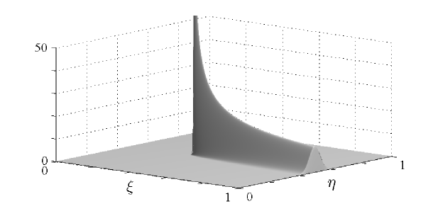
Figure 5.1: Typical behaviour of the Green’s function $G(\frac{1}{3},\frac{1}{2};\cdot,\cdot)$ for problem (5.1) with $b=1$, $c=0$ and $\varepsilon=10^{-3}$.

shows a representation of a Green’s function $G(1/3,1/2;\cdot,\cdot)$ for a small value of $\varepsilon=10^{-3}$ and coefficients $b=1$ and $c=0$. The singularity at $(\xi,\eta)=(x,y)$ and strong anisotropic behaviour of $G$ can be seen quite nicely. Near the boundary $\xi=1$ the Green’s function has a strong boundary layer – an outflow boundary layer.

The unique solution $u$ of (5.1) has the representation

$$u(x,y)=\iint_{\Omega}G(x,y;\xi,\eta)\,f(\xi,\eta)\,d\xi\,d\eta.$$ (5.2)

Our goal is to use (5.2) and $L_{1}$-norm estimates of $G$ to obtain pointwise error bounds of $u-u^{N}$, where $u^{N}$ is the numerical solution of a certain method. By using this idea, we get a-posteriori error bounds with computable terms.

In a more general numerical-analysis context, we note that sharp estimates for continuous Green’s functions (or their generalised versions) frequently play a crucial role in a priori and a posteriori error analyses [11, 28, 49].

The main result for $L_{1}$-norm bounds on $G$ is the following from [20].

Theorem 5.1 (Theorem 2.2 of [20]).

Let $\varepsilon\in(0,1]$. The Green’s function $G(x,y;\xi,\eta)$ associated with (5.1) on the unit square $\Omega=(0,1)^{2}$ satisfies, for any $(x,y)\in\Omega$, the following bounds

$$\|{\partial_{\xi}G(x,y;\cdot)}\|_{L_{1}(\Omega)} \leq C(1+|\ln\varepsilon|), \|{\partial_{\eta}G(x,y;\cdot)}\|_{L_{1}(\Omega)} \leq C\varepsilon^{-1/2}.$$ (5.3a)

Furthermore, for any ball $$B(x^{\prime},y^{\prime};\rho) \rho (x^{\prime},y^{\prime})\in\bar{\Omega}$$ of radius centred at any , we have

$$\|{G(x,y;\cdot)}\|_{W_{1}^{1}(B(x^{\prime},y^{\prime};\rho))} \leq C\varepsilon^{-1}\rho,$$ (5.3b)

while for the ball $$B(x,y;\rho) \rho (x,y)$$ of radius centred at we have

$$\|{\partial^{2}_{\xi}G(x,y;\cdot)}\|_{L_{1}(\Omega\setminus B(x,y;\rho))} \leq C\varepsilon^{-1}\ln(2+\varepsilon/\rho),$$ (5.3c)

$$\|{\partial^{2}_{\eta}G(x,y;\cdot)}\|_{L_{1}(\Omega\setminus B(x,y;\rho))} \leq C\varepsilon^{-1}(\ln(2+\varepsilon/\rho)+|\ln\varepsilon|).$$ (5.3d)

Let us compare the first order results to those obtained in one dimension, see e.g. [41, Theorems 3.23, 3.31]. Here we have for the Green’s function $g^{cd}$ of a convection-diffusion problem

$$\|{\partial_{\xi}g^{cd}(x;\cdot)}\|_{L_{1}(\Omega)}\leq C$$

and for $g^{rd}$ of a reaction-diffusion problem

$$\|{\partial_{\xi}g^{rd}(x;\cdot)}\|_{L_{1}(\Omega)}\leq C\varepsilon^{-1/2}.$$

Comparing these results with the results of Theorem 5.1, we see an additional dependence on $|\ln\varepsilon|$ in the streamline derivative. Thus the question for sharpness of these estimates is legitimate. In [19] it is shown that above bounds are sharp w.r.t. $\varepsilon$.

Theorem 5.2 (Theorem 3 of [19]).

Let $\varepsilon\in(0,c_{0}]$ for some sufficiently small positive $c_{0}$. The Green’s function $G$ associated with the constant-coefficient problem (5.1) in the unit square $\Omega=(0,1)^{2}$ satisfies, for all $(x,y)\in[\frac{1}{4},\frac{3}{4}]^{2}$, the following lower bounds: There exists a constant $\underline{c}>0$ independent of $\varepsilon$ such that

$$\|{\partial_{\xi}G(x,y;\cdot)}\|_{L_{1}(\Omega)} \geq\underline{c}|\ln\varepsilon|, \|{\partial_{\eta}G(x,y;\cdot)}\|_{L_{1}(\Omega)} \geq\underline{c}\varepsilon^{-1/2}.$$ (5.4a)

Furthermore, for any ball $$B(x,y;\rho) \rho\leq\frac{1}{8}$$ of radius , we have

$$\|{G(x,y;\cdot)}\|_{W_{1}^{1}(\Omega\cap B(x,y;\rho))} \geq\begin{cases}\underline{c}\rho/\varepsilon,&\mbox{if\leavevmode\nobreak\ }\rho\leq 2\varepsilon,\\ \underline{c}(\rho/\varepsilon)^{1/2},&\mbox{otherwise},\\ \end{cases}$$ (5.4b)

$$\|{\partial^{2}_{\xi}G(x,y;\cdot)}\|_{L_{1}(\Omega\setminus B(x,y;\rho))} \geq\underline{c}\varepsilon^{-1}\ln(2+\varepsilon/\rho),\quad \mbox{if\leavevmode\nobreak\ }\rho\leq c_{1}\varepsilon,$$ (5.4c)

$$\|{\partial^{2}_{\eta}G(x,y;\cdot)}\|_{L_{1}(\Omega\setminus B(x,y;\rho))} \geq\underline{c}\varepsilon^{-1}(\ln(2+\varepsilon/\rho)+|\ln\varepsilon|), \mbox{if\leavevmode\nobreak\ }\rho\leq{\textstyle\frac{1}{8}},$$ (5.4d)

where $$c_{1}$$ is a sufficiently small positive constant.

Not that the restriction $(x,y)\in[\frac{1}{4},\frac{3}{4}]^{2}$ can be replaced by $(x,y)\in[\theta,1-\theta]^{2}$ with $\theta\in(0,\frac{1}{2})$. Doing so, we have to replace $\rho\leq\frac{1}{8}$ by $\rho\leq\frac{1}{2}\theta$.

Above results have been proved in 2d and 3d in [20, 19, 18]. The basic idea is to look at a frozen coefficient version of (5.1) and to analyse the behaviour of its fundamental solution and of the difference to the fundamental solution of the original problem. This approach is sometimes called parametrix method. The results can be generalised to arbitrary dimensions, say $n\in\mathbb{N}$. In order to do so, let us denote by $\underline{\mathbf{x}}=(x_{1},x_{2},\dots,x_{n})$ a vector in $\mathbb{R}^{n}$ and by $K_{s}$ the modified Bessel function of second kind and order $s$ with $s\in\mathbb{R}$.

The basic idea is to look at the fundamental solution of

$$\bar{L}^{*}_{\underline{\mathbf{\xi}}}\bar{g}(\underline{\mathbf{x}};\underline{\mathbf{\xi}})=-\varepsilon\Delta_{\underline{\mathbf{\xi}}}\bar{g}+b(\underline{\mathbf{x}})\bar{g}_{\xi_{1}} =\delta(\underline{\mathbf{x}}-\underline{\mathbf{\xi}}),\quad\underline{\mathbf{\xi}}\in\mathbb{R}^{n}$$ (5.5)

where $\delta(\cdot)$ is the $n$-dimensional Dirac-distribution. For fixed $\underline{\mathbf{x}}$ the coefficient $b(\underline{\mathbf{x}})$ in (5.5) is constant and we can solve the problem explicitly. To simplify our presentation, let $q=\frac{1}{2}b(\underline{\mathbf{x}})$ for fixed $\underline{\mathbf{x}}\in(0,1)^{n}$. Now a transformation, see [30], can be used to change the type of the problem from convection-diffusion to reaction-diffusion. For reaction-diffusion problems with constant coefficients the fundamental solution is known and we obtain the fundamental solution of (5.5) as

$$\bar{g}(\underline{\mathbf{x}};\underline{\mathbf{\xi}})=\frac{1}{(2\pi)^{n/2}\varepsilon^{n-1}}\,\left(\frac{q}{\hat{r}}\right)^{n/2-1}e^{q\hat{\xi}_{1}}K_{n/2-1}(q\hat{r}),\qquad q=q(\underline{\mathbf{x}})={\textstyle\frac{1}{2}}b(\underline{\mathbf{x}})$$

where $\hat{r}=\|{\underline{\mathbf{\xi}}-\underline{\mathbf{x}}}\|_{2}/\varepsilon$ and $\hat{\xi}_{k}=(\xi_{k}-x_{k})/\varepsilon$. Note that for $n=2$ we obtain

$$\bar{g}_{2}(x,y;\xi,\eta)=\frac{1}{2\pi\varepsilon}\,e^{q\hat{\xi}_{1}}K_{0}(q\hat{r}),\qquad q=q(x,y)={\textstyle\frac{1}{2}}b(x,y),$$

the fundamental solution used in [20] and for $n=3$

$$\bar{g}_{3}(\underline{\mathbf{x}};\underline{\mathbf{\xi}})=\frac{1}{(2\pi)^{3/2}\varepsilon^{2}}\,\left(\frac{q}{\hat{r}}\right)^{1/2}e^{q\hat{\xi}_{1}}K_{1/2}(q\hat{r})=\frac{1}{4\pi\varepsilon^{2}}\,\frac{e^{q(\xi_{1}-x_{1}-r)/\varepsilon}}{\hat{r}},\qquad q=q(\underline{\mathbf{x}})={\textstyle\frac{1}{2}}b(\underline{\mathbf{x}}),$$

the fundamental solution used in [18].

The modified Bessel functions $K_{s}$ of order $s$ and those of order zero behave asymptotically very similar, see [50, Sections 10.25 to 10.60]. Therefore, to modify the analysis presented in [20, 19, 18] to the $n$-dimensional case is straightforward, though tedious and we obtain the analogue to Theorem 5.1 and 5.2 also in the $n$-dimensional case.

5.2 A-Posteriori Error Estimation

Here we want to apply the $L_{1}$-norms of the Green’s function and derive a-posteriori error estimates in the $L_{\infty}$-norm. The analysis following is from the forthcoming paper [17]. Note, that in this section derivatives are to be understood in the sense of distributions.

Let the domain $\Omega$ be discretised by a rectangular tensor-product mesh $T$ with the nodes $(x_{i},y_{j})$, where $0=x_{0}<x_{1}<\ldots<x_{N}=1$ and $0=y_{0}<y_{1}<\ldots<y_{M}=1$ for $N,M\in\mathbb{N}$. On this mesh we derive the main ingredient of an a-posteriori error estimator, an $(L_{\infty},W_{-1,\infty})$-stability result, following [35, Theorem 4.1].

Theorem 5.3.

Let $u$ be the unique solution of (5.1) for a given right-hand side $f$ satisfying

$$f(x,y)=\bar{f}(x,y)-\frac{\partial}{\partial x}[F_{1}(x,y)+\bar{F}_{1}(x,y)]-\frac{\partial}{\partial y}[F_{2}(x,y)+\bar{F}_{2}(x,y)]$$ (5.6)

where

$$F_{1}(x,y)|_{(x_{i-1},x_{i})} =A_{i}(y)(x-x_{i-1/2}), i=1,\dots,N$$

$$F_{2}(x,y)|_{(y_{j-1},y_{j})} =B_{j}(x)(y-y_{j-1/2}), j=1,\dots,M$$

and $\bar{f},\,\bar{F}_{1},\,\bar{F}_{2},\,A_{i},$ and $B_{j}$ are arbitrary functions in $L_{\infty}(\Omega)$.

Then it holds that

$$\|{u}\|_{L_{\infty}(\Omega)}\leq C\bigg{[} \|{\bar{f}}\|_{L_{\infty}(\Omega)}+(1+|\ln\varepsilon|)\|{\bar{F}_{1}}\|_{L_{\infty}(\Omega)}+\varepsilon^{-1/2}\|{\bar{F}_{2}}\|_{L_{\infty}(\Omega)}+$$

$$\max_{i=1,\dots,N}\left\{\min\left\{h_{i}^{2}\frac{\ln(2+\varepsilon/\kappa_{h})}{\varepsilon},h_{i}(1+|\ln\varepsilon|)\right\}\max_{y\in[0,1]}|A_{i}(y)|\right\}+$$

$$\max_{j=1,\dots,M}\left\{\min\left\{k_{j}^{2}\frac{|\ln\varepsilon|+\ln(2+\varepsilon/\kappa_{k})}{\varepsilon},\frac{k_{j}}{\varepsilon^{1/2}}\right\}\max_{x\in[0,1]}|B_{j}(x)|\right\}\bigg{]}$$

with $\kappa_{h}=\min h_{i},\,\kappa_{k}=\min k_{j}$.

Remark 5.4.

The existence of $u\in L_{\infty}(\Omega)$ for a given right-hand side $f$ of the form (5.6) follows from the classical results [36, Chap. 3 Theorems 5.2, 13.1].

Proof of Theorem 5.3.

Using the linearity of the operator $L$, we split $f$ into different parts and analyse them separately. For simplicity of the representation, denote by $g(\xi,\eta)=G(x,y;\xi,\eta)$.

1) Let $\mathbf{\bar{F}_{1}=\bar{F}_{2}=F_{1}=F_{2}=0}$, i.e. $f=\bar{f}$.
The maximum principle (or (5.2) and $\|{g}\|_{L_{1}(\Omega)}\leq C$) implies

$$\|{u}\|_{L_{\infty}(\Omega)}\leq C\|{\bar{f}}\|_{L_{\infty}(\Omega)}.$$

2) Let $\mathbf{\bar{f}=F_{1}=F_{2}=0}$, i.e. $f=-\frac{\partial}{\partial x}\bar{F}_{1}-\frac{\partial}{\partial y}\bar{F}_{2}$.
We represent $u$ using (5.2). Integration by parts and a Cauchy-Schwarz inequality give

$$u(x,y) =\iint_{\Omega}g(\xi,\eta)f(\xi,\eta)d\xi d\eta$$

$$=\iint_{\Omega}g_{\xi}(\xi,\eta)\bar{F}_{1}(\xi,\eta)d\xi d\eta+\iint_{\Omega}g_{\eta}(\xi,\eta)\bar{F}_{2}(\xi,\eta)d\xi d\eta$$

$$\leq\|{G_{\xi}}\|_{L_{1}(\Omega)}\|{\bar{F}_{1}}\|_{L_{\infty}(\Omega)}+\|{G_{\eta}}\|_{L_{1}(\Omega)}\|{\bar{F}_{2}}\|_{L_{\infty}(\Omega)}.$$

With (5.3a) we obtain

$$\|{u}\|_{L_{\infty}(\Omega)}\leq C\left[(1+|\ln\varepsilon|)\|{\bar{F}_{1}}\|_{L_{\infty}(\Omega)}+\varepsilon^{-1/2}\|{\bar{F}_{2}}\|_{L_{\infty}(\Omega)}\right].$$

3) Let $\mathbf{\bar{f}=\bar{F}_{1}=\bar{F}_{2}=F_{2}=0}$, $f=-\frac{\partial}{\partial x}F_{1}$.
Using (5.2) and integration by parts again, we have

$$u(x,y) =\iint_{\Omega}F_{1}(\xi,\eta)g_{\xi}(\xi,\eta)d\xi d\eta=\sum_{i=1}^{N}\iint_{\Omega_{i}}A_{i}(\eta)(\xi-\xi_{i-1/2})g_{\xi}(\xi,\eta)d\xi d\eta$$

where $\Omega_{i}=(x_{i-1},x_{i})\times[0,1]$. The Green’s function $g$ has a singularity at $(x,y)$. Define $0<n<N$ where $x\in[x_{n-1/2},x_{n+1/2}]$ and $\Omega^{\prime}=(x_{n-1},x_{n+1})\times(y-\tilde{h}_{n},y+\tilde{h}_{n})$ where $\tilde{h}_{n}=\min\{h_{n},h_{n+1}\}/2$. Note that the singularity now lies in $\Omega^{\prime}$.

Defining the singularity-free function $\tilde{g}$ by $\tilde{g}=g$ in $\Omega\setminus\Omega^{\prime}$ and $\tilde{g}=0$ in $\Omega^{\prime}$ we obtain

$$u(x,y) =\sum_{i=1}^{N}\iint_{\Omega_{i}}\!\!\!\!A_{i}(\eta)(\xi-\xi_{i-1/2})\tilde{g}_{\xi}(\xi,\eta)d\xi d\eta+\sum_{i=n}^{n+1}\iint_{\Omega_{i}\cap\Omega^{\prime}}\!\!\!\!\!A_{i}(\eta)(\xi-\xi_{i-1/2})g_{\xi}(\xi,\eta)d\xi d\eta$$

$$=:S_{1}+S_{2}.$$

The term $S_{1}$ can be estimated in two different ways. Either by

$$\left|\int_{x_{i-1}}^{x_{i}}\!\!(\xi-x_{i-1/2})\tilde{g}_{\xi}(\xi,\eta)d\xi\right| \leq\frac{h_{i}}{2}\int_{x_{i-1}}^{x_{i}}|\tilde{g}_{\xi}(\xi,\eta)|d\xi$$

or by

$$\left|\int_{x_{i-1}}^{x_{i}}\!\!(\xi-x_{i-1/2})\tilde{g}_{\xi}(\xi,\eta)d\xi\right| =\left|\int_{x_{i-1}}^{x_{i}}\!\!(\xi-x_{i-1/2})\int_{x_{i-1}}^{\xi}\!\!\tilde{g}_{\xi\xi}(s,\eta)dsd\xi\right|\leq\frac{h_{i}^{2}}{4}\int_{x_{i-1}}^{x_{i}}\!\!|\tilde{g}_{\xi\xi}(\xi,\eta)|d\xi.$$

Note that $\tilde{g}_{\xi\xi}$ is well defined. In order to use these two possibilities, decompose $A_{i}=A_{i}^{1}+A_{i}^{2}$ where

$$A_{i}^{1}=\begin{cases}A_{i},&2h_{i}\varepsilon(1+|\ln\varepsilon|)\leq h_{i}^{2}\ln(2+\varepsilon/\kappa_{h})\\ 0,&\mbox{otherwise}\end{cases}\quad\mbox{and }A_{i}^{2}=A_{i}-A_{i}^{1}.$$

This yields by using Theorem 5.1

$$|S_{1}| \leq\sum_{i=1}^{N}\int_{0}^{1}|A_{i}(\eta)|\left|\int_{x_{i-1}}^{x_{i}}(\xi-\xi_{i-1/2})\tilde{g}_{\xi}(\xi,\eta)d\xi\right|d\eta$$

$$\leq\max_{i=1,\dots,N}\left\{\frac{h_{i}}{2}\max_{\eta\in[0,1]}|A_{i}^{1}(\eta)|\right\}\iint_{\Omega\setminus\Omega^{\prime}}|G_{\xi}(\xi,\eta)|d\xi d\eta+$$

$$\hskip 14.22636pt\max_{i=1,\dots,N}\left\{\frac{h_{i}^{2}}{4}\max_{\eta\in[0,1]}|A_{i}^{2}(\eta)|\right\}\iint_{\Omega\setminus\Omega^{\prime}}|G_{\xi\xi}(\xi,\eta)|d\xi d\eta$$

$$\leq C\max_{i=1,\dots,N}\left\{\min\left\{h_{i}(1+|\ln\varepsilon|),\frac{h_{i}^{2}}{\varepsilon}\ln(2+\varepsilon/\kappa_{h})\right\}\max_{\eta\in[0,1]}|A_{i}(\eta)|\right\}.$$

For $S_{2}$ we use either (5.3a)

$$\|{G_{\xi}}\|_{L_{1}(\Omega)}\leq C(1+|\ln\varepsilon|)$$

or (5.3b)

$$\|{G_{\xi}}\|_{L_{1}(B(a,b,\rho))}\leq C\varepsilon^{-1}\rho.$$

Let $A_{i}=\tilde{A}_{i}^{1}+\tilde{A}_{i}^{2}$ with

$$\tilde{A}_{i}^{1}=\begin{cases}A_{i},&h_{i}\varepsilon(1+|\ln\varepsilon|)\leq h_{i}^{2}\\ 0,&\mbox{otherwise}\end{cases}\quad\mbox{and }\tilde{A}_{i}^{2}=A_{i}-\tilde{A}_{i}^{1}.$$

Then holds

$$|S_{2}| \leq\sum_{i=n}^{n+1}\iint_{\Omega_{i}\cap\Omega^{\prime}}|A_{i}(\eta)||(\xi-\xi_{i-1/2})||g_{\xi}(\xi,\eta)|d\xi d\eta$$

$$\leq\sum_{i=n}^{n+1}\frac{h_{i}}{2}\max_{\eta\in[0,1]}|A_{i}(\eta)|\iint_{B(x_{i-1/2},y,h_{i})}|g_{\xi}(\xi,\eta)|d\xi d\eta$$

$$\leq C\left(\max_{i=n,n+1}\left\{\frac{h_{i}}{2}\max_{\eta\in[0,1]}|\tilde{A}_{i}^{1}(\eta)|\right\}|\ln\varepsilon|+\max_{i=n,n+1}\left\{\frac{h_{i}^{2}}{2\varepsilon}\max_{\eta\in[0,1]}|\tilde{A}_{i}^{2}(\eta)|\right\}\right)$$

$$\leq C\max_{i=n,n+1}\left\{\min\left\{h_{i}(1+|\ln\varepsilon|),\frac{h_{i}^{2}}{\varepsilon}\right\}\max_{\eta\in[0,1]}|A_{i}(\eta)|\right\}.$$

Thus we obtain

$$\|{u}\|_{L_{\infty}(\Omega)}\leq C\max_{i=1,\dots,N}\left\{\min\left\{h_{i}(1+|\ln\varepsilon|),\frac{h_{i}^{2}}{\varepsilon}\ln(2+\varepsilon/\kappa_{h})\right\}\max_{\eta\in[0,1]}|A_{i}(\eta)|\right\}.$$

4) Let $\mathbf{\bar{f}=\bar{F}_{1}=F_{1}=\bar{F}_{2}=0}$, i.e. $f=-\frac{\partial}{\partial y}F_{2}$.
This case can be treated similarly to the one above. Using a similar splitting of $u=\widetilde{S}_{1}+\widetilde{S}_{2}$ gives

$$|\widetilde{S}_{1}| \leq C\max_{j=1,\dots,M}\left\{\min\left\{\frac{k_{j}}{\varepsilon^{1/2}},\frac{k_{j}^{2}}{\varepsilon}(|\ln\varepsilon|+\ln(2+\varepsilon/\kappa_{k}))\right\}\max_{\xi\in[0,1]}|B_{j}(\xi)|\right\}$$

and

$$|\widetilde{S}_{2}| \leq C\max_{j=m,m+1}\left\{\min\left\{\frac{k_{j}}{\varepsilon^{1/2}},\frac{k_{j}^{2}}{\varepsilon}\right\}\max_{\xi\in[0,1]}|B_{j}(\xi)|\right\}$$

and therefore

$$\|{u}\|_{L_{\infty}(\Omega)}\leq C\max_{j=1,\dots,M}\left\{\min\left\{\frac{k_{j}}{\varepsilon^{1/2}},\frac{k_{j}^{2}}{\varepsilon}(|\ln\varepsilon|+\ln(2+\varepsilon/\kappa_{k}))\right\}\max_{\xi\in[0,1]}|B_{j}(\xi)|\right\}.$$

By combining these estimates the stability result is proved. ∎

Note that in above results the global minima $\kappa_{h}$ and $\kappa_{k}$ can be replaced by local minima over two adjacent cells each.

Application to an Upwind Method

So far our Green’s function estimates have not been applied to finite element methods. The Green’s function $G$ is in general not in $H_{0}^{1}(\Omega)$ which complicates the derivation of uniform a-posteriori error estimators via above approach. Further research is needed to apply this approach to finite element methods.

Instead, we will apply the stability result to an upwind finite difference method. Let us start by rewriting (5.1) as

$$Lu =-(A_{1}u)_{x}-(A_{2}u)_{y}-(Bu)_{x}+Cu=f$$ (5.7a)

where

$$A_{1}u =\varepsilon u_{x},\quad A_{2}u=\varepsilon u_{y},\quad Bu=bu\quad\mbox{and}\quad Cu=cu.$$ (5.7b)

Using the index sets $I=\{1,\dots,N-1\}$, $\bar{I}=\{0,\dots,N\}$, $J=\{1,\dots,M-1\}$ and $\bar{J}=\{0,\dots,M\}$, we define our discrete counterpart to (5.7):

$$L^{N}\mathbf{u}_{ij}= -\widetilde{D}_{x}A_{1}^{N}\mathbf{u}_{ij}-\widetilde{D}_{y}A_{2}^{N}\mathbf{u}_{ij}-\widetilde{D}_{x}B^{N}\mathbf{u}_{ij}+C^{N}\mathbf{u}_{ij}$$

$$= -\varepsilon(D_{x}^{2}\mathbf{u}_{ij}+D_{y}^{2}\mathbf{u}_{ij})-\widetilde{D}_{x}(\mathbf{b}_{ij}\mathbf{u}_{ij})+\mathbf{c}_{ij}\mathbf{u}_{ij}\quad=\mathbf{f}_{ij}, i\in I,j\in J$$ (5.8a)

$$\mathbf{u}_{i,0}= \,\mathbf{u}_{i,M}=0, i\in\bar{I}$$ (5.8b)

$$\mathbf{u}_{0,j}= \,\mathbf{u}_{N,j}=0, j\in\bar{J}.$$ (5.8c)

where

$$\mathbf{f}_{ij} =f(x_{i},y_{j})$$

$$A_{1}^{N}\mathbf{u}_{ij} =\varepsilon D^{-}_{x}\mathbf{u}_{ij},\quad A_{2}^{N}\mathbf{u}_{ij}=\varepsilon D^{-}_{y}\mathbf{u}_{ij},\quad B^{N}\mathbf{u}_{ij}=\mathbf{b}_{ij}\mathbf{u}_{ij}\quad\mbox{and}\quad C^{N}\mathbf{u}_{ij}=\mathbf{c}_{ij}\mathbf{u}_{ij}$$

with the standard backward difference operators $D^{-}$. With $\hbar_{i}=(h_{i}+h_{i+1})/2$ the other discrete operators are defined as

$$\widetilde{D}_{x}\mathbf{u}_{ij} =\frac{\mathbf{u}_{i+1,j}-\mathbf{u}_{ij}}{\hbar_{i}}, D_{x}^{2}\mathbf{u}_{ij} =\frac{1}{\hbar_{i}}\left[\frac{\mathbf{u}_{i+1,j}-\mathbf{u}_{ij}}{h_{i+1}}-\frac{\mathbf{u}_{i,j}-\mathbf{u}_{i-1,j}}{h_{i}}\right], i\in I,\,j\in J,$$

and similarly in $y$-direction.

Note that (5.8) is a non-standard upwind finite difference method. The difference to the standard upwind FDM is the treatment of the convective term by $\widetilde{D}_{x}$ instead of $D^{+}_{x}$. The reason for this different treatment lies in the following analysis.

Let us use the continuous residual, i.e. $L(\mathbf{u}^{\mathcal{B}}-u)$. Here $\mathbf{u}^{\mathcal{B}}$ denotes the piecewise bilinear interpolant of the discrete variable $\mathbf{u}$. With $\mathbf{u}^{\mathcal{I}}$ and $\mathbf{u}^{\mathcal{J}}$ as the one-dimensional piecewise linear interpolations in $x$- and $y$-direction, respectively we have

$$\mathbf{u}^{\mathcal{B}}=(\mathbf{u}^{\mathcal{I}})^{\mathcal{J}}=(\mathbf{u}^{\mathcal{J}})^{\mathcal{I}}.$$

With a proper extension of our discrete operators to the boundary of $\Omega$, it holds for the residual

$$L(\mathbf{u}^{\mathcal{B}}-u) =-\left[(A_{1}\mathbf{u}^{\mathcal{I}})_{x}+\mathbf{F_{1}}^{\mathcal{I}}\right]^{\mathcal{J}}-\left[(A_{2}\mathbf{u}^{\mathcal{J}})_{y}+\mathbf{F_{2}}^{\mathcal{J}}\right]^{\mathcal{I}}$$

$$\quad-\left[(B\mathbf{u}^{\mathcal{I}})_{x}+\mathbf{F_{3}}^{\mathcal{I}}\right]^{\mathcal{J}}+\left[C\mathbf{u}^{\mathcal{B}}-\mathbf{F_{4}}^{\mathcal{B}}\right]-f+\mathbf{f}^{\mathcal{B}}$$ (5.9)

where

$$\mathbf{F_{1}}_{ij} :=-\widetilde{D}_{x}A_{1}^{N}\mathbf{u}_{ij}, \mathbf{F_{2}}_{ij} :=-\widetilde{D}_{y}A_{2}^{N}\mathbf{u}_{ij},$$

$$\mathbf{F_{3}}_{ij} :=-\widetilde{D}_{x}B^{N}\mathbf{u}_{ij}, \mathbf{F_{4}}_{ij} :=C^{N}\mathbf{u}_{ij}.$$

Let us start with the first term on the right-hand side of (5.9) for $x\in[x_{i-1},x_{i}]$ and fixed $y=y_{j}$. With the auxiliary terms

$$Q^{1} :=\int_{x}^{1}\mathbf{F_{1}}^{\mathcal{I}}, Q^{1}_{i} :=\sum_{k=i}^{N-1}\mathbf{F_{1}}_{kj}\hbar_{k}$$

we obtain

$$Q^{1}_{i}=A_{1}^{N}\mathbf{u}_{ij}-A_{1}^{N}\mathbf{u}_{Nj}=A_{1}^{N}\mathbf{u}_{ij}$$

and therefore

$$(A_{1}\mathbf{u}^{\mathcal{I}})_{x}+\mathbf{F_{1}}^{\mathcal{I}}=\partial_{x}(A_{1}\mathbf{u}^{\mathcal{I}}-Q^{1})=\partial_{x}(A_{1}\mathbf{u}^{\mathcal{I}}-A_{1}^{N}\mathbf{u}_{ij})+\partial_{x}(Q^{1}_{i}-Q^{1})=\partial_{x}(Q^{1}_{i}-Q^{1}).$$

Now using the summation in $Q^{1}_{i}$ we can estimate further

$$\partial_{x}(Q^{1}_{i}-Q^{1}) =\partial_{x}\left(\int_{x_{i}}^{1}\mathbf{F_{1}}^{\mathcal{I}}-\int_{x}^{1}\mathbf{F_{1}}^{\mathcal{I}}+\mathbf{F_{1}}_{ij}\frac{h_{i}}{2}-\mathbf{F_{1}}_{Nj}\frac{h_{N}}{2}\right)$$

$$=\partial_{x}\left(-\int_{x}^{x_{i}}\mathbf{F_{1}}^{\mathcal{I}}+\mathbf{F_{1}}_{ij}\frac{h_{i}}{2}\right)$$

$$=\partial_{x}\left(\mathbf{F_{1}}_{ij}\frac{(x-x_{i-1})^{2}}{2h_{i}}-\mathbf{F_{1}}_{i-1,j}\frac{(x_{i}-x)^{2}}{2h_{i}}\right).$$

Thus we obtain

$$-\left[(A_{1}\mathbf{u}^{\mathcal{I}})_{x}+\mathbf{F_{1}}^{\mathcal{I}}\right]^{\mathcal{J}}\bigg{|}_{x\in[x_{i-1},x_{i}]}=-\partial_{x}\left(\mathbf{F_{1}}_{ij}\frac{(x-x_{i-1})^{2}}{2h_{i}}-\mathbf{F_{1}}_{i-1,j}\frac{(x_{i}-x)^{2}}{2h_{i}}\right)^{\mathcal{J}}.$$ (5.10)

With similar techniques the other terms of (5.9) can be rewritten. Note that (5.10) can be further transformed to yield second-order terms in $h_{i}$ but then we obtain discrete third-order derivatives. We apply this for the $y$-derivatives. Now using the stability result of Theorem 5.3 to the right-hand side of the continuous residual (5.9) yields an a-posteriori error estimator.

Theorem 5.5.

Let $\mathbf{u}$ be the solution of (5.8) and $u$ be the solution of (5.1). Then holds

$$\|{\mathbf{u}^{\mathcal{B}}-u}\|_{L_{\infty}(\Omega)} \leq C\bigg{(}\max_{\stackrel{{\scriptstyle i=0,\dots,N}}{{j=1,\dots,M}}}M^{1}_{ij}+\max_{\stackrel{{\scriptstyle i=0,\dots,N}}{{j=1,\dots,M}}}M^{2}_{ij}+\max_{\stackrel{{\scriptstyle i=0,\dots,N}}{{j=1,\dots,M}}}M^{3}_{ij}+$$

$$\hskip 34.14322pt\max_{\stackrel{{\scriptstyle i=1,\dots,N}}{{j=0,\dots,M}}}M^{4}_{ij}+\max_{\stackrel{{\scriptstyle i=1,\dots,N}}{{j=0,\dots,M}}}M^{5}_{ij}+\max_{\stackrel{{\scriptstyle i=1,\dots,N}}{{j=0,\dots,M}}}M^{6}_{ij}+\max_{\stackrel{{\scriptstyle i=1,\dots,N}}{{j=0,\dots,M}}}M^{7}_{ij}\bigg{)}$$

with the terms depending on discrete $$y$$-derivatives

$$M_{ij}^{1} :=\min\{\varepsilon^{1/2}k_{j},k_{j}^{2}(|\ln\varepsilon|+\ln(2+\varepsilon/\kappa_{k}))\}\min\{|D_{y}^{2}\mathbf{u}_{i,j-1}|,|D_{y}^{2}\mathbf{u}_{ij}|\},$$

$$M_{ij}^{2} :=\varepsilon^{1/2}k_{j}^{2}|D_{y}^{-}D_{y}^{2}\mathbf{u}_{i,j}|,$$

$$M_{ij}^{3} :=k_{j}^{2}(1+|D_{y}^{-}\mathbf{u}_{ij}|^{2}),$$

and terms depending on discrete $$x$$-derivatives

$$M_{ij}^{4} :=\varepsilon h_{i}(1+|\ln\varepsilon|)\max\{|[D_{x}^{2}\mathbf{u}]_{i-1,j}|,|[D_{x}^{2}\mathbf{u}]_{ij}|\},$$

$$M_{ij}^{5} :=h_{i}^{2}(1+|[D_{x}^{-}\mathbf{u}]_{ij}|^{2}),$$

$$M_{ij}^{6} :=h_{i}(1+|\ln\varepsilon|)\max\{|[\widetilde{D}_{x}\mathbf{u}]_{i-1,j}|,|[\widetilde{D}_{x}\mathbf{u}]_{ij}|\},$$

$$M_{ij}^{7} :=h_{i}(1+|\ln\varepsilon|)(1+|[D_{x}^{-}\mathbf{u}]_{ij}|).$$

Note that formally, $M^{1}$ to $M^{3}$ are of order $k_{j}^{2}$ while $M^{4}$, $M^{6}$ and $M^{7}$ are of order $h_{i}$. Only $M^{5}$ is of order $h_{i}^{2}$ and therefore probably negligible. Thus, the estimator is formally of first order (if $k_{j}^{2}\leq h_{i}$) which is consistent with the formal order of an upwind method.

The constant $C$ in the error bound of Theorem 5.5 is unknown. By setting it to $C=1$ we obtain an error indicator that gives us information about the convergence behaviour, though not about the exact value of the error. For singularly perturbed problems the uniformity of the indicator is usually more important than the precise value of $C$.

Remark 5.6.

The part $M^{2}$ contains discrete third-order derivatives. They are costly to evaluate and therefore an estimator with only second-order derivatives would be beneficial. In [34, §6] an idea is used, that bounds the third-order derivative by a second-order derivative term. This approach could be used here too. We will tackle it in the forthcoming paper [17].

A Numerical Example

Let us consider the numerical example

$$-\varepsilon\Delta u-u_{x}+\frac{1}{2}u =f \text{in }\Omega=(0,1)^{2},$$ (5.11a)

$$u =0 \text{on }\partial\Omega,$$ (5.11b)

where the right-hand side $$f$$ is chosen such that

$$u(x,y)=\left(\cos\frac{\pi x}{2}-\frac{\mathrm{e}^{-x/\varepsilon}-\mathrm{e}^{-1/\varepsilon}}{1-\mathrm{e}^{-1/\varepsilon}}\right)\frac{\left(1-\mathrm{e}^{-y/\sqrt{\varepsilon}}\right)\left(1-\mathrm{e}^{-(1-y)/\sqrt{\varepsilon}}\right)}{1-\mathrm{e}^{-1/\sqrt{\varepsilon}}}$$ (5.11c)

is the solution.

Dependence on $\varepsilon$

In our first experiment we look into the uniformity w.r.t. $\varepsilon$ of the indicator given in Theorem 5.5 with $C=1$. For given values of $\varepsilon$ we compute the numerical solution on an a-priori chosen Shishkin mesh for $N=64$ and compare the results in Figure 5.2.

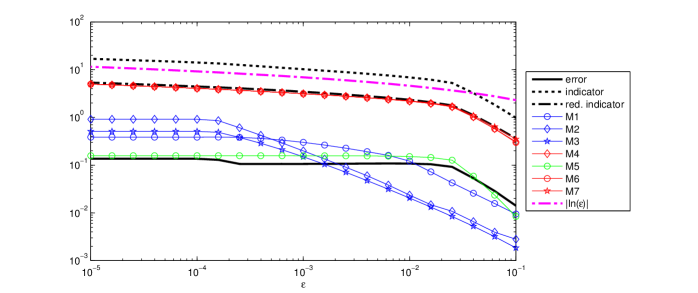
Figure 5.2: Error and estimated error of (5.11) for $N=64$ on a Shishkin mesh

Therein for each component of the indicator a line is shown. Additionally, a solid black line represents the real error, and a black dash-dot line represents a modified indicator. The modified indicator takes only the maxima of $M^{1}$, $M^{3}$, $M^{4}$ and $M^{7}$. In numerical simulations this modification represents the behaviour of the error much better than the real indicator. For another motivation, see also Remark 5.6.

In Figure 5.2 both indicators behave like $|\ln\varepsilon|$, which is also given for comparison as a line in magenta. But the real error stays almost constant for $\varepsilon$ becoming smaller. Thus, there is a $|\ln\varepsilon|$-dependence in our estimators coming from the Green’s function estimates, although they are sharp. This behaviour was seen for several different examples.

As a consequence we will use from now on the heuristic indicator

$$\eta :=\bigg{(}\max_{\stackrel{{\scriptstyle i=0,\dots,N}}{{j=1,\dots,M}}}M^{1}_{ij}+\max_{\stackrel{{\scriptstyle i=0,\dots,N}}{{j=1,\dots,M}}}M^{2}_{ij}+\max_{\stackrel{{\scriptstyle i=0,\dots,N}}{{j=1,\dots,M}}}M^{3}_{ij}+$$

$$\hskip 34.14322pt\max_{\stackrel{{\scriptstyle i=1,\dots,N}}{{j=0,\dots,M}}}M^{4}_{ij}+\max_{\stackrel{{\scriptstyle i=1,\dots,N}}{{j=0,\dots,M}}}M^{5}_{ij}+\max_{\stackrel{{\scriptstyle i=1,\dots,N}}{{j=0,\dots,M}}}M^{6}_{ij}+\max_{\stackrel{{\scriptstyle i=1,\dots,N}}{{j=0,\dots,M}}}M^{7}_{ij}\bigg{)}$$

and the modified indicator

$$\widetilde{\eta} :=\bigg{(}\max_{\stackrel{{\scriptstyle i=0,\dots,N}}{{j=1,\dots,M}}}M^{1}_{ij}+\max_{\stackrel{{\scriptstyle i=0,\dots,N}}{{j=1,\dots,M}}}M^{3}_{ij}+\max_{\stackrel{{\scriptstyle i=1,\dots,N}}{{j=0,\dots,M}}}M^{4}_{ij}+\max_{\stackrel{{\scriptstyle i=1,\dots,N}}{{j=0,\dots,M}}}M^{7}_{ij}\bigg{)}$$

where

$$M_{ij}^{1} :=\min\{\varepsilon^{1/2}k_{j},k_{j}^{2}\ln(2+\varepsilon/\kappa_{k})\}\min\{|D_{y}^{2}\mathbf{u}_{i,j-1}|,|D_{y}^{2}\mathbf{u}_{ij}|\},$$

$$M_{ij}^{2} :=\varepsilon^{1/2}k_{j}^{2}|D_{y}^{-}D_{y}^{2}\mathbf{u}_{i,j}|,\qquad\qquad M_{ij}^{3}:=k_{j}^{2}(1+|D_{y}^{-}\mathbf{u}_{ij}|^{2}),$$

$$M_{ij}^{4} :=\varepsilon h_{i}\max\{|[D_{x}^{2}\mathbf{u}]_{i-1,j}|,|[D_{x}^{2}\mathbf{u}]_{ij}|\},$$

$$M_{ij}^{5} :=h_{i}^{2}(1+|[D_{x}^{-}\mathbf{u}]_{ij}|^{2}),\qquad\qquad M_{ij}^{6}:=h_{i}\max\{|[\widetilde{D}_{x}\mathbf{u}]_{i-1,j}|,|[\widetilde{D}_{x}\mathbf{u}]_{ij}|\},$$

$$M_{ij}^{7} :=h_{i}(1+|[D_{x}^{-}\mathbf{u}]_{ij}|).$$

Figure 5.3

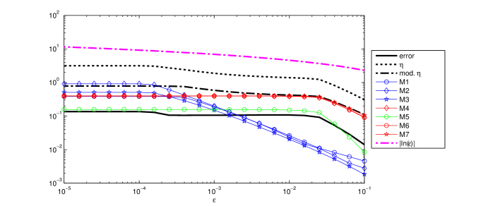
Figure 5.3: Error and modified estimated error of (5.11) for $N=64$ on a Shishkin mesh

shows the behaviour of these modified indicators. Obviously, there is no dependence on $\varepsilon$ any longer and the errors are caught quite well.

Convergence in $N$ on a-priori adapted meshes

For our second experiment we let $\varepsilon=10^{-6}$ be constant, chose a-priori adapted meshes, apply the modified upwind method and estimate the error with $\eta$ and $\widetilde{\eta}$. Figures 5.4

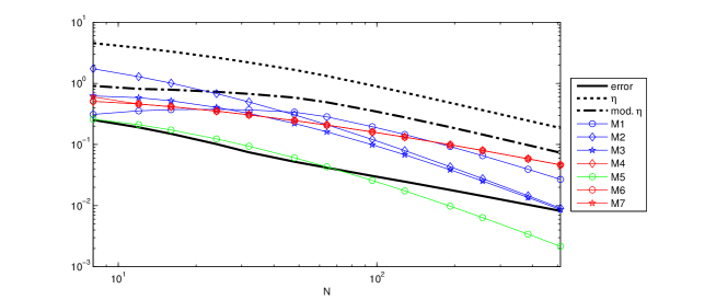
Figure 5.4: Error and estimated error of (5.11) for $\varepsilon=10^{-6}$ on Shishkin meshes

and 5.5

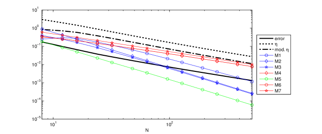
Figure 5.5: Error and estimated error of (5.11) for $\varepsilon=10^{-6}$ on a Bakhvalov S-meshes

show the results for the two indicators and variable $N$. The principal behaviour of the errors is caught by both of them although the magnitude is wrong. We also observe the blue lines to fall much faster than the red lines. The reason behind is the formal second order convergence in $y$-direction of $M^{1}$ to $M^{3}$. This gives hope for a-posteriori mesh adaptation to behave better than a-priori adapted meshes.

A-posteriori adapted meshes

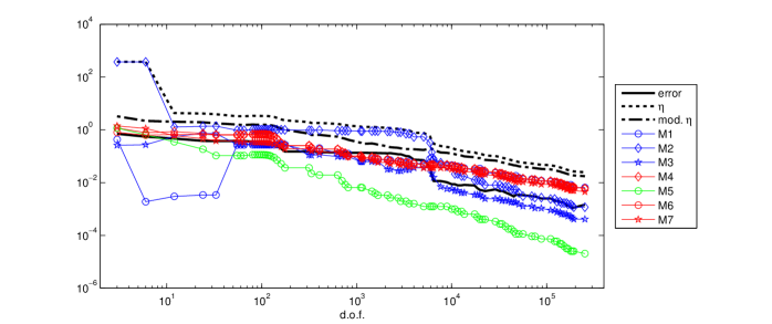
Figure 5.6: Error and estimated error of (5.11) for $\varepsilon=10^{-6}$ on an adapted mesh with initial Shishkin mesh

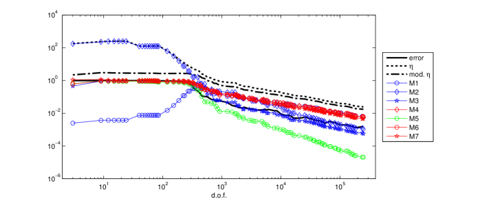
Figure 5.7: Error and estimated error of (5.11) for $\varepsilon=10^{-6}$ on an adapted mesh with initial equidistant mesh

Let us consider the following simple, anisotropic mesh adaptation approach. We start with a coarse initial, tensor-product mesh. In each step we compute the numerical solution on the given mesh and use the error indicators to decide, whether and where the $x$-part or the $y$-part of the tensor product mesh should be refined. This will be done as follows:

1. Compute $M_{y}:=\max\limits_{k=1,3}\{\max\{M_{ij}^{k}\}\}$ and $M_{x}:=\max\limits_{k=4,5,6,7}\{\max\{M_{ij}^{k}\}\}$.

2. If $M_{x}>M_{y}$ we refine in $x$-direction, otherwise in $y$-direction. Assuming $M_{x}>M_{y}$ we collect all $i$ with $M_{ij}^{k}\geq\alpha\max\{M_{ij}^{k}\}$ for any $k=4,5,6,7$ and given $\alpha\in[0,1]$, and divide $[x_{i-1},x_{i}]$ into two intervals of equal length. Similarly, we proceed in the other case and divide $[y_{j-1},y_{j}]$ into two intervals for all $j$ with $M_{ij}^{k}\geq\alpha\max\{M_{ij}^{k}\}$ for any $k=1,2,3$.

With these refined partitions we construct a new tensor product mesh and the cycle begins again. This refinement process has a parameter $\alpha$ influencing the marking of elements to refine. We chose $\alpha=0.9$ to refine only elements with large contributions.

In Figure 5.6 and 5.7 the convergence results for $\varepsilon=10^{-6}$ are shown until the number of degrees of freedom reaches approximately $512^{2}$. In Figure 5.6 initially a Shishkin mesh of 4-by-4 cells was taken and in the end we have $1014\times 250$ cells. In Figure 5.7 the initial mesh was equidistant with 4-by-4 cells, and the final mesh has $992\times 252$ cells.

We observe in both cases that our adaptation process reduces the error nicely. The observed overall order of convergence (after some initial phase) is $(\#dof)^{-1/2}$ where $\#dof$ is the number of degrees of freedom.

Comparing the errors for the number of degrees of freedom taken to be about $512^{2}$, Table 5.1

Table 5.1: Comparison of errors of a-priori and a-posteriori meshes

mesh	$\#dof$	$\|{\mathbf{u}^{\mathcal{B}}-u}\|_{L_{\infty}(\Omega)}$
Shishkin-mesh	262144	8.2024e-03
Bakhvalov S-mesh	262144	1.3226e-03
adapted mesh with initial S-mesh	253500	1.4570e-03
adapted mesh with initial equidistant mesh	249984	1.5117e-03

shows the results on the a-posteriori adapted meshes to be comparable to the a-priori adapted meshes. With the different number of cells in each direction the a-posteriori adapted meshes can reduce the error much better than a Shishkin mesh. Still, the grading of the Bakhvalov S-mesh gives a mesh with the smallest error. Moreover, the costs for an adaptive algorithm are high due to the repeated solving of the numerical problems on the different meshes.

Chapter 6 Conclusion and Outlook

We have presented convergence and supercloseness results for higher-order finite-element methods, including stabilised methods like LPSFEM and SDFEM. Having general polynomial spaces $\mathcal{Q}^{\clubsuit}_{p}$, convergence of order $p$ can be proved. If we use proper subspaces of $\mathcal{Q}_{p}$, like the Serendipity space, we cannot apply the supercloseness techniques that are valid for the full space $\mathcal{Q}_{p}$. But numerical results do also indicate, that for proper subspaces no supercloseness property holds.

While numerical simulations indicate supercloseness properties of order $p+1$ for many methods, numerical analysis provides proof only for order $p+1/2$ in the case of SDFEM. Further research is needed to improve this situation. Some preliminary results for the pure Galerkin method are topic of ongoing research. Here a supercloseness property in the case of exponential boundary layers and odd polynomial degree $p$ of order $p+1/4$ could be proved, [26]. The proof therein can easily be adapted to the case of characteristic boundary layers too. Nevertheless, there is still a gap between theory and simulation of $3/4$ orders.

Although convergence and supercloseness can be proved in the energy and related norms, these norms do not “see” the characteristic layers correctly. The layers are under-represented in the resulting terms. An alternative is shown in the balanced norm that has the right weighting of the norm components. But now the Galerkin FEM is no longer coercive w.r.t. this norm. Using certain stability arguments, for a modified bilinear SDFEM convergence in this norm is proved. How the proof can be modified for the standard Galerkin FEM and other stabilised methods, and for higher order methods in general is an open question. Numerically, all these methods show the same convergence and supercloseness behaviour in the energy and the balanced norm.

The use of a-priori adapted meshes requires knowledge about the layer-structure of solutions to the considered problem. Alternatively, the mesh can be adapted after computation of an (approximative) numerical solution. For this a-posteriori mesh adaptation, uniform error estimators or indicators are needed. We presented estimates on the $L_{1}$-norm of the Green’s function as an ingredient for $L_{\infty}$-error estimators. A simple, first estimator for a finite difference method is also given and analysed. The optimisation of this estimator and an extension of this approach to finite element methods are open problems. Bibliography

Appendix

Appendix pages=1-1, pagecommand=

S. Franz, G. Matthies: Local projection stabilisation on S-type meshes for convection-diffusion problems with characteristic layers. Computing, 87(3-4), 135–167, 2010

[The article is removed from this electronic version due to copyright reasons.]

Abstract:

Singularly perturbed convection-diffusion problems with exponential and characteristic layers are considered on the unit square. The discretisation is based on layer-adapted meshes. The standard Galerkin method and the local projection scheme are analysed for bilinear and higher order finite element where enriched spaces were used. For bilinears, first order convergence in the $\varepsilon$-weighted energy norm is shown for both the Galerkin and the stabilised scheme. However, supercloseness results of second orders hold for the Galerkin method in the $\varepsilon$-weighted energy norm and for the local projection scheme in the corresponding norm. For the enriched $\mathcal{Q}_{p}$-elements, $p\geq 2$, which already contain the space $\mathcal{P}_{p+1}$, a convergence order $p+1$ in the $\varepsilon$-weighted energy norm is proved for both the Galerkin method and the local projection scheme. Furthermore, the local projection methods provides a supercloseness result of order $p+1$ in local projection norm.

Keywords: Singular perturbation, Characteristic layers, Shishkin meshes, Local projection

Mathematics Subject Classification (2000): 65N12, 65N30, 65N50

DOI: 10.1007/s00607-010-0079-y

S. Franz, G. Matthies: Convergence on Layer-adapted Meshes and Anisotropic Interpolation Error Estimates of Non-Standard Higher Order Finite Elements. Appl. Numer. Math., 61, 723–737, 2011

[The article is removed from this electronic version due to copyright reasons.]

Abstract:

For a general class of finite element spaces based on local polynomial spaces $\mathcal{E}$ with $\mathcal{P}_{p}\subset\mathcal{E}\subset\mathcal{Q}_{p}$ we construct a vertex-edge-cell and point-value oriented interpolation operators that fulfil anisotropic interpolation error estimates.

Using these estimates we prove $\varepsilon$-uniform convergence of order $p$ for the Galerkin FEM and the LPSFEM for a singularly perturbed convection-diffusion problem with characteristic boundary layers.

Keywords: singular perturbation, characteristic layers, exponential layers, Shishkin meshes, local-projection, higher-order FEM

Mathematics Subject Classification (2000): 65N12, 65N30, 65N50

DOI: 10.1016/j.apnum.2011.02.001

S. Franz: Superconvergence Using Pointwise Interpolation in Convection-Diffusion Problems. Appl. Numer. Math., 76, 132–144, 2014

[The article is removed from this electronic version due to copyright reasons.]

Abstract:

Considering a singularly perturbed convection-diffusion problem, we present an analysis for a superconvergence result using pointwise interpolation of Gauß-Lobatto type for higher-order streamline diffusion FEM. We show a useful connection between two different types of interpolation, namely a vertex-edge-cell interpolant and a pointwise interpolant. Moreover, different postprocessing operators are analysed and applied to model problems.

Keywords: singular perturbation, layer-adapted meshes, superconvergence, postprocessing

Mathematics Subject Classification (2000): 65N12, 65N30, 65N50

DOI: 10.1016/j.apnum.2013.07.007

S. Franz: SDFEM with non-standard higher-order finite elements for a convection-diffusion problem with characteristic boundary layers. BIT Numerical Mathematics, 51(3), 631–651, 2011

[The article is removed from this electronic version due to copyright reasons.]

Abstract:

Considering a singularly perturbed problem with exponential and characteristic layers, we show convergence for non-standard higher-order finite elements using the streamline diffusion finite element method (SDFEM). Moreover, for the standard higher-order space $\mathcal{Q}_{p}$ supercloseness of the numerical solution w.r.t. an interpolation of the exact solution in the streamline diffusion norm of order $p+1/2$ is proved.

Keywords: singular perturbation, characteristic layers, exponential layers, Shishkin mesh, SDFEM, higher order

Mathematics Subject Classification (2000): 65N12, 65N30, 65N50

DOI: 10.1007/s10543-010-0307-z

S. Franz: Convergence Phenomena of $Q_{p}$-Elements for Convection-Diffusion Problems. Numer. Methods Partial Differential Equations, 29(1), 280–296, 2013

[The article is removed from this electronic version due to copyright reasons.]

Abstract:

We present a numerical study for singularly perturbed convection-diffusion problems using higher-order Galerkin and Streamline Diffusion FEM. We are especially interested in convergence and superconvergence properties with respect to different interpolation operators. For this we investigate pointwise interpolation and vertex-edge-cell interpolation.

Keywords: singular perturbation, boundary layers, layer-adapted meshes, superconvergence

Mathematics Subject Classification (2000): 65N12, 65N30, 65N50

DOI: 10.1002/num.21709

S. Franz, H.-G. Roos: Error estimation in a balanced norm for a convection-diffusion problem with characteristic boundary layers. Calcolo, DOI:10.1007/s10092-013-0093-5, 2013

[The article is removed from this electronic version due to copyright reasons.]

Abstract:

The $\varepsilon$-weighted energy norm is the natural norm for singularly perturbed convection-diffusion problems with exponential layers. But, this norm is too weak to recognise features of characteristic layers.

We present an error analysis in a differently weighted energy norm—a balanced norm—that overcomes this drawback.

Keywords: singular perturbation, characteristic and exponential layers, Shishkin mesh, SDFEM, balanced norm

Mathematics Subject Classification (2000): 65N12, 65N30, 65N50

DOI: 10.1007/s10092-013-0093-5

S. Franz, N. Kopteva: Green’s function estimates for a singularly perturbed convection-diffusion problem. Journal of Differential Equations, 252, 1521–1545, 2012

[The article is removed from this electronic version due to copyright reasons.]

Abstract:

We consider a singularly perturbed convection-diffusion problem posed in the unit square with a horizontal convective direction. Its solutions exhibit parabolic and exponential boundary layers. Sharp estimates of the Green’s function and its first- and second-order derivatives are derived in the $L_{1}$ norm. The dependence of these estimates on the small diffusion parameter is shown explicitly. The obtained estimates will be used in a forthcoming numerical analysis of the considered problem.

Keywords: Green’s function, singular perturbations, convection-diffusion

Mathematics Subject Classification (2000): 35J08, 35J25, 65N15

DOI: 10.1016/j.jde.2011.07.033

S. Franz, N. Kopteva: On the Sharpness of Green’s function estimates for a convection-diffusion problem. In Proceedings of the Fifth Conference on Finite Difference Methods: Theory and Applications (FDM: T&A 2010), 44–57, Rousse University Press, 2011

[The article is removed from this electronic version due to copyright reasons.]

Abstract:

Linear singularly perturbed convection-diffusion problems with characteristic layers are considered in three dimensions. We demonstrate the sharpness of our recently obtained upper bounds for the associated Green’s function and its derivatives in the $L_{1}$ norm. For this, in this paper we establish the corresponding lower bounds. Both upper and lower bounds explicitly show any dependence on the singular perturbation parameter.

Keywords: Green’s function, singular perturbations, convection-diffusion, a posteriori error estimates

Mathematics Subject Classification (2000): 35J08, 35J25, 65N15

ISBN: 978-954-8467-44-5

Erklärung

Hiermit versichere ich, dass ich die vorliegene Arbeit ohne unzulässige Hilfe Dritter und ohne Benutzung anderer als der angegebenen Hilsmittel angefertigt habe. Die aus fremden Quellen direkt oder indirekt übernommenen Gedanken sind als solche kenntlich gemacht. Die Arbeit wurde bisher weder im In- noch im Ausland in gleicher oder ähnlicher Form einer anderen Prüfungsbehörde vorgelegt.

Dresden, den 31.05.2013.

References

- [1] T. Apel. Anisotropic finite elements: local estimates and applications. Advances in Numerical Mathematics. B. G. Teubner, Stuttgart, 1999.
- [2] D. N. Arnold and G. Awanou. The Serendipity Family of Finite Elements. Found. Comput. Math., 11: 337–344, 2011.
- [3] D. N. Arnold, D. Boffi, R. S. Falk and L. Gastaldi. Finite element approximation on quadrilateral meshes. Comm. Numer. Methods Engrg., 17(11): 805–812, 2001.
- [4] N. S. Bakhvalov. The optimization of methods of solving boundary value problems with a boundary layer. U.S.S.R. Comput. Math. Math. Phys., 9(4): 139–166, 1969.
- [5] R. Becker and M. Braack. A finite element pressure gradient stabilization for the Stokes equations based on local projections. Calcolo, 38(4): 173–199, 2001.
- [6] R. Becker and M. Braack. A two-level stabilization scheme for the Navier-Stokes equations. In M. Feistauer, V. Dolejší, P. Knobloch and K. Najzar, editors, Numerical mathematics and advanced applications, 123–130. Springer-Verlag, Berlin, 2004.
- [7] M. Braack and E. Burman. Local projection stabilization for the Oseen problem and its interpretation as a variational multiscale method. SIAM J. Numer. Anal., 43(6): 2544–2566, 2006.
- [8] L. Chen and J. Xu. Stability and accuracy of adapted finite element methods for singularly perturbed problems. Numer. Math., 109(2): 167–191, 2008.
- [9] R. G. Durán and A. L. Lombardi. Finite element approximation of convection diffusion problems using graded meshes. Appl. Numer. Math., 56: 1314–1325, 2006.
- [10] R. G. Durán, A. L. Lombardi and M. I. Prieto. Supercloseness on graded meshes for finite element approximation of a reaction–diffusion equation. J. Comp. Appl. Math., 242: 232–247, 2013.
- [11] K. Eriksson. An adaptive finite element method with efficient maximum norm error control for elliptic problems. Math. Models Methods Appl. Sci., 4: 313–329, 1994.
- [12] S. Franz. Continuous interior penalty method on a Shishkin mesh for convection-diffusion problems with characteristic boundary layers. Comput. Meth. Appl. Mech. Engng., 197(45-48): 3679–3686, 2008.
- [13] S. Franz. Singularly perturbed problems with characteristic layers: Supercloseness and postprocessing. Ph.D. thesis, Department of Mathematics, TU Dresden, 2008. http://nbn-resolving.de/urn:nbn:de:bsz:14-ds-1218629566251-73654.
- [14] S. Franz. SDFEM with non-standard higher-order finite elements for a convection-diffusion problem with characteristic boundary layers. BIT Numerical Mathematics, 51(3): 631–651, 2011.
- [15] S. Franz. Convergence Phenomena of -Elements for Convection-Diffusion Problems. Numer. Methods Partial Differential Equations, 29(1): 280–296, 2013.
- [16] S. Franz. Superconvergence using pointwise interpolation in convection-diffusion problems. Appl. Numer. Math., 76: 132–144, 2014.
- [17] S. Franz and N. Kopteva. Uniform a-posteriori estimates for a convection-diffusion problem with characteristic boundary layers. In preparation.
- [18] S. Franz and N. Kopteva. Green’s function estimates for a singularly perturbed convection-diffusion problem in three dimensions. Int. J. Numer. Anal. Model. Ser. B, 2(2-3): 124–141, 2011.
- [19] S. Franz and N. Kopteva. On the sharpness of Green’s function estimates for a convection-diffusion problem. In M. Koleva and L. Vulkov, editors, Proceedings of the Fifth Conference on Finite Difference Methods: Theory and Applications (FDM: T&A 2010), 44–57. Rousse University Press, 2011. ArXiv:1102.4520v2.
- [20] S. Franz and N. Kopteva. Green’s function estimates for a singularly perturbed convection-diffusion problem. J. Differential Equations, 252: 1521–1545, 2012.
- [21] S. Franz and T. Linß. Superconvergence analysis of the Galerkin FEM for a singularly perturbed convection-diffusion problem with characteristic layers. Numer. Methods Partial Differential Equations, 24(1): 144–164, 2008.
- [22] S. Franz, T. Linß and H.-G. Roos. Superconvergence analysis of the SDFEM for elliptic problems with characteristic layers. Appl. Numer. Math., 58(12): 1818–1829, 2008.
- [23] S. Franz and G. Matthies. Local projection stabilisation on S-type meshes for convection-diffusion problems with characteristic layers. Computing, 87(3-4): 135–167, 2010.
- [24] S. Franz and G. Matthies. Convergence on Layer-Adapted Meshes and Anisotropic Interpolation Error Estimates of Non-Standard Higher Order Finite Elements. Appl. Numer. Math., 61(01/10): 723–737, 2011.
- [25] S. Franz and H.-G. Roos. Error estimation in a balanced norm for a convection-diffusion problem with two different boundary layers. Calcolo, 2013. DOI:10.1007/s10092-013-0093-5.
- [26] S. Franz and H.-G. Roos. Superconvergence for Higher-Order Elements in Convection-Diffusion Problems. Numer. Math. Theor. Meth. Appl., 2014. Accepted for publication, arXiv:1307.7543.
- [27] V. Girault and P. Raviart. Finite element methods for Navier-Stokes equations: Theory and Algorithms. Springer series in computational mathematics. Springer-Verlag, Berlin, Heidelberg, New York, 1986.
- [28] J. Guzmán, D. Leykekhman, J. Rossmann and A. H. Schatz. Hölder estimates for Green’s functions on convex polyhedral domains and their applications to finite element methods. Numer. Math., 112: 221–243, 2009.
- [29] T. J. R. Hughes and A. N. Brooks. A multidimensional upwind scheme with no crosswind diffusion. In Finite element methods for convection dominated flows (Papers, Winter Ann. Meeting Amer. Soc. Mech. Engrs., New York, 1979), volume 34 of AMD, 19–35. Amer. Soc. Mech. Engrs. (ASME), New York, 1979.
- [30] R. B. Kellogg and S. Shih. Asymptotic analysis of a singular perturbation problem. SIAM Journal on Mathematical Analysis, 18(5): 1467–1510, 1987.
- [31] R. B. Kellogg and M. Stynes. Sharpened and corrected version of: Corner singularities and boundary layers in a simple convection-diffusion problem. J. Differential Equations, 213(1): 81–120, 2005.
- [32] R. B. Kellogg and M. Stynes. Sharpened bounds for corner singularities and boundary layers in a simple convection-diffusion problem. Appl. Math. Lett., 20(5): 539–544, 2007.
- [33] P. Knobloch. A Generalization of the Local Projection Stabilization for Convection-Diffusion-Reaction Equations. SIAM J. Numer. Anal., 48(2): 659–680, 2010.
- [34] N. Kopteva. Maximum norm a posteriori error estimate for a one-dimensional singularly perturbed semilinear reaction-diffusion problem. IMA J. Numer. Anal., 27: 576–592, 2007.
- [35] N. Kopteva. Maximum norm a posteriori error estimate for a 2d singularly perturbed reaction-diffusion problem. SIAM J. Numer. Anal., 46: 1602–1618, 2008.
- [36] O. A. Ladyzhenskaya and N. N. Ural’tseva. Linear and Quasilinear Elliptic Equations. Academic Press, New York, 1968.
- [37] B. Li. Lagrange interpolation and finite element superconvergence. Numer. Methods Partial Differential Equations, 20(1): 33–59, 2004.
- [38] Q. Lin, N. Yan and A. Zhou. A rectangle test for interpolated element analysis. In Proc. Syst. Sci. Eng., 217–229. Great Wall (H.K.) Culture Publish Co., 1991.
- [39] R. Lin and M. Stynes. A balanced finite element method for singularly perturbed reaction-diffusion problems. SIAM J. Numerical Analysis, 50(5): 2729–2743, 2012.
- [40] T. Linß. Analysis of a Galerkin finite element method on a Bakhvalov-Shishkin mesh for a linear convection-diffusion problem. IMA J. Numer. Anal., 20(4): 621–632, 2000.
- [41] T. Linß. Layer-adapted meshes for reaction-convection-diffusion problems, volume 1985 of Lecture Notes in Mathematics. Springer, Heidelberg, Berlin, 2010.
- [42] T. Linß and M. Stynes. Asymptotic analysis and Shishkin-type decomposition for an elliptic convection-diffusion problem. J. Math. Anal. Appl., 261(2): 604–632, 2001.
- [43] T. Linß and M. Stynes. Numerical methods on Shishkin meshes for linear convection-diffusion problems. Comput. Methods Appl. Mech. Eng., 190(28): 3527–3542, 2001.
- [44] G. Matthies. Local projection methods on layer-adapted meshes for higher order discretisations of convection-diffusion problems. Appl. Numer. Math., 59(10): 2515–2533, 2009.
- [45] G. Matthies. Local projection stabilisation for higher order discretisations of convection-diffusion problems on Shishkin meshes. Adv. Comput. Math., 30(4): 315–337, 2009.
- [46] G. Matthies, P. Skrzypacz and L. Tobiska. A unified convergence analysis for local projection stabilisations applied to the Oseen problem. M2AN Math. Model. Numer. Anal., 41(4): 713–742, 2007.
- [47] J. Melenk. hp-Finite Element Methods for Singular Perturbations, volume 1796 of Lecture Notes in Mathematics. Springer, Berlin, 2003.
- [48] J. J. H. Miller, E. O’Riordan and G. I. Shishkin. Fitted numerical methods for singular perturbation problems: Error estimates in the maximum norm for linear problems in one and two dimensions. World Scientific Publishing Co. Inc., River Edge, NJ, 1996.
- [49] R. H. Nochetto. Pointwise a posteriori error estimates for elliptic problems on highly graded meshes. Math. Comp., 64: 1–22, 1995.
- [50] F. Olver, D. Lozier, R. F. Boisvert and C. Clark. NIST Handbook of Mathematical Functions. Cambridge University Press, Cambridge, 2010.
- [51] H.-G. Roos. Optimal convergence of basic schemes for elliptic boundary value problems with strong parabolic layers. Journal of Mathematical Analysis and Applications, 267(1): 194 – 208, 2002.
- [52] H.-G. Roos and T. Linß. Sufficient conditions for uniform convergence on layer-adapted grids. Computing, 63(1): 27–45, 1999.
- [53] H.-G. Roos and M. Schopf. Convergence and stability in balanced norms of finite element methods on Shishkin meshes for reaction-diffusion problems. ZAMM, 2014. Accepted for publication.
- [54] H.-G. Roos, M. Stynes and L. Tobiska. Robust numerical methods for singularly perturbed differential equations, volume 24 of Springer Series in Computational Mathematics. Springer, Berlin, second edition, 2008.
- [55] M. Stynes and E. O’Riordan. A uniformly convergent Galerkin method on a Shishkin mesh for a convection-diffusion problem. J. Math. Anal. Appl., 214(1): 36–54, 1997.
- [56] M. Stynes and L. Tobiska. The SDFEM for a convection-diffusion problem with a boundary layer: optimal error analysis and enhancement of accuracy. SIAM J. Numer. Anal., 41(5): 1620–1642, 2003.
- [57] M. Stynes and L. Tobiska. Using rectangular elements in the SDFEM for a convection-diffusion problem with a boundary layer. Appl. Numer. Math., 58(12): 1709–1802, 2008.
- [58] P. Sun, L. Chen and J. Xu. Numerical Studies of Adaptive Finite Element Methods for Two Dimensional Convection-Dominated Problems. J. Sci. Comput., 43: 24–43, 2010.
- [59] B. Szabó and I. Babuška. Finite Element Analysis. John Wiley and Sons, New York, 1991.
- [60] L. Tobiska. Analysis of a new stabilized higher order finite element method for advection-diffusion equations. Comput. Methods Appl. Mech. Engrg., 196: 538–550, 2006.
- [61] M. van Veldhuizen. Higher order methods for a singularly perturbed problem. Numer. Math., 30: 267–279, 1978.
- [62] Z. Zhang. Finite element superconvergence on Shishkin mesh for 2-d convection-diffusion problems. Math. Comp., 72(243): 1147–1177, 2003.
- [63] M. Zlámal. Superconvergence and Reduced Integration in the Finite Element Method. Math. Comp., 32(143): 663–685, 1978.