Equation of state of a relativistic theory from a moving frame

Abstract

We propose a new strategy for determining the equation of state of a relativistic thermal quantum field theory by considering it in a moving reference system. In this frame an observer can measure the entropy density of the system directly from its average total momentum. In the Euclidean path integral formalism, this amounts to compute the expectation value of the off-diagonal components $T_{0k}$ of the energy-momentum tensor in presence of shifted boundary conditions. The entropy is thus easily measured from the expectation value of a local observable computed at the target temperature $T$ only. At large $T$, the temperature itself is the only scale which drives the systematic errors, and the lattice spacing can be tuned to perform a reliable continuum limit extrapolation while keeping finite-size effects under control. We test this strategy for the four-dimensional $SU(3)$ Yang-Mills theory. We present precise results for the entropy density and its step-scaling function in the temperature range $0.9\,T_{c}-20\,T_{c}$. At each temperature, we consider four lattice spacings in order to extrapolate the results to the continuum limit. As a byproduct we also determine the ultraviolet finite renormalization constant of $T_{0k}$ by imposing suitable Ward identities. These findings establish this strategy as a solid, simple and efficient method for an accurate determination of the equation of state of a relativistic thermal field theory over several orders of magnitude in $T$.

Introduction.— Relativistic thermal quantum field theories are of central importance in many areas of research in physics. The equation of state (EOS) of Quantum Chromo Dynamics (QCD) is a very basic property of strongly-interacting matter that is of absolute interest in particle and nuclear physics, and in cosmology. It is also a crucial input in the analysis of data collected at the heavy-ion colliders.
Lattice QCD is the only known theoretical framework where the EOS can be determined from first principles in the interesting range of temperature values. Since the perturbative expansion converges very slowly, the full computation of the EOS has to be done numerically over several orders of magnitude in $T$. Severe unphysical contributions hinder the standard way of computing the pressure and the energy density. The expansion of the free energy in the bare parameters, and the subtraction of ultraviolet power divergences make the computation of the EOS technically difficult and numerically very demanding Boyd et al. (1996); Borsanyi et al. (2012); Cheng et al. (2010); Borsanyi et al. (2013) (see Ref. Philipsen (2013) for a recent review). Temperatures higher than a few hundreds MeV are still unreachable with staggered fermions. The computation remains prohibitive with Wilson fermions. The obstacles, however, are not rooted in the physics content of the EOS, but in the strategy adopted for its computation. This calls for a conceptual progress able to trigger new computational strategies, which in turn are capable to reach the goal of a precise computation of the EOS in a generic discretization of the theory.
The underlying Lorentz symmetry of relativistic thermal theories offers an elegant and simple solution to this problem. In these theories the entropy is proportional to the total momentum of the system as measured by an observer in a moving frame. Remarkably, the corresponding Euclidean path integral formulation is rather simple. It corresponds to inserting a shift ${\bm{\xi}}$ in the spatial directions when closing the boundary conditions of a field $\phi$ in the compact direction of length $L_{0}$ Giusti and Meyer (2013, 2011a, 2011b); Della Morte and Giusti (2011)

$$\phi(L_{0},{\bm{x}})=\phi(0,{\bm{x}}-L_{0}\,{\bm{\xi}})\;.$$ (1)

In the thermodynamic limit, the invariance of the dynamics under the $SO(4)$ group implies that the free energy density $f(L_{0},{\bm{\xi}})$ satisfies Giusti and Meyer (2013, 2011a, 2011b)

$$f(L_{0},{\bm{\xi}})=f(L_{0}\sqrt{1+{\bm{\xi}}^{2}},{\bm{0}})\;.$$ (2)

Hence the free energy does not depend on $L_{0}$ and ${\bm{\xi}}$ separately but on the combination $L_{0}\sqrt{1+{\bm{\xi}}^{2}}=T^{-1}$ which fixes the inverse temperature of the system. This redundancy implies that the thermal distributions of the total energy and momentum are related, and interesting Ward identities (WIs) follow. In particular, the entropy density can be written as Giusti and Meyer (2013)

$$\frac{s(T)}{T^{3}}=-\frac{(1+{\bm{\xi}}^{2})}{\xi_{k}}\frac{\langle T_{0k}\rangle_{\bm{\xi}}}{T^{4}}\;,$$ (3)

where $\langle\cdot\rangle_{\bm{\xi}}$ stands for the expectation value computed with a non-zero shift ${\bm{\xi}}$. No ultraviolet power-divergent contributions need to be subtracted from $\langle T_{0k}\rangle_{\bm{\xi}}$.

In this Letter we explore a new computational strategy for determining the EOS of a relativistic thermal quantum field theory based on Eq. (3). We illustrate the power of the method in the $SU(3)$ Yang-Mills theory, where we determine the entropy density of the system in the range $0.9\,T_{c}-20\,T_{c}$. This is a particularly interesting theory since it is the limit of QCD in absence of fermions (or with infinitely heavy fermions), and it can be used to test new ideas and numerical methods without facing the problems of simulating dynamical fermions. Since it relies on Lorentz invariance only, the strategy is directly applicable to any relativistic thermal theory and, in particular, to QCD.
Entropy density from the lattice.— We regularize the four-dimensional $SU(3)$ Yang–Mills theory on a square lattice of size $L_{0}\times L^{3}$ and of spacing $a$. The link variables $U_{\mu}(x)\in SU(3)$ represent the gauge field and the Wilson action $S$ is, up to a constant, given by

$$S[U]=-\frac{\beta}{6}\!\sum_{x,\mu\nu}\!\mbox{Re}\,\hbox{\rm Tr}[U_{\mu}(x)U_{\nu}(x+\hat{\mu})U^{\dagger}_{\mu}(x+\hat{\nu})U^{\dagger}_{\nu}(x)]$$

where $\beta=6/g_{0}^{2}$, and $g_{0}$ is the bare coupling. We impose periodic boundary conditions in the spatial directions and shifted boundary conditions along the compact direction, $U_{\mu}(L_{0},{\bm{x}})=U_{\mu}(0,{\bm{x}}-L_{0}\,{\bm{\xi}})$, where $(L_{0}/a)\,{\bm{\xi}}$ is a vector with integer components. We consider the clover definition of the energy-momentum tensor on the lattice Caracciolo et al. (1990)

$$T_{\mu\nu}=\frac{\beta}{6}\Big{\{}F^{a}_{\mu\alpha}F^{a}_{\nu\alpha}-\frac{1}{4}\delta_{\mu\nu}F^{a}_{\alpha\beta}F^{a}_{\alpha\beta}\Big{\}}\;.$$ (4)

The field strength tensor is defined as

$$F^{a}_{\mu\nu}(x)=-\frac{i}{4a^{2}}\,\hbox{\rm Tr}\Big{\{}\Big{[}Q_{\mu\nu}(x)-Q_{\nu\mu}(x)\Big{]}T^{a}\Big{\}}\;,$$ (5)

where $T^{a}=\lambda^{a}/2$ with $\lambda^{a}$ being the Gell-Mann matrices, and (see Ref. Caracciolo et al. (1990) for more details)

$$Q_{\mu\nu}(x)=P_{\mu\nu}(x)+P_{\nu-\mu}(x)+P_{-\mu-\nu}(x)+P_{-\nu\mu}(x)\;.$$ (6)

The matrix $P_{\mu\nu}(x)$ is the parallel transport along an elementary plaquette at the lattice site $x$ along the directions $\mu$ and $\nu$, and the minus sign stands for the negative orientation. The lattice regularization breaks explicitly translation invariance down to a discrete sub-group. As a consequence the off-diagonal components of the energy-momentum tensor renormalize multiplicatively Caracciolo et al. (1990), and Eq. (3) becomes

$$\frac{s(T)}{T^{3}}=-\frac{(1+{\bm{\xi}}^{2})}{\xi_{k}}\,\frac{Z_{T}\langle T_{0k}\rangle_{\bm{\xi}}}{T^{4}}\;.$$ (7)

The renormalization constant $Z_{T}$ of $T_{0k}$ can be fixed by imposing suitable WIs Giusti and Meyer (2011a, 2013). $Z_{T}$ depends only on the bare coupling constant and, up to discretization effects, it is independent of the kinematic parameters e.g., $L$, $T$, ${\bm{\xi}}$. These parameters can be chosen at will, with the condition that they remain constant in physical units when approaching the continuum limit, or that they generate in $Z_{T}$ negligible discretization effects compared to the statistical errors. Ultimately, which WI and/or kinematics are the most effective has to be investigated numerically. We have found that for the $SU(3)$ Yang–Mills theory discretized with the Wilson action, $Z_{T}$ can be determined with small discretization effects and with a limited numerical effort as

$$Z_{T}=\frac{1}{2aL^{3}}\frac{1}{\langle T_{0k}\rangle_{{\bm{\xi}}}}\ln{\frac{Z(L_{0},{\bm{\xi}}+a/L_{0}\hat{k})}{Z(L_{0},{\bm{\xi}}-a/L_{0}\hat{k})}}\;,$$ (8)

where $Z(L_{0},{\bm{\xi}})$ is the partition function of the theory. Once $Z_{T}$ is known, the lattice size and spacing can be adjusted so to carry out a reliable continuum limit extrapolation of the entropy density at any given value of $T$ with moderate computational resources. This is possible thanks to the fact that at large $T$ the temperature itself is the only relevant scale that drives discretization and finite volume effects. The mass gap of the theory is proportional to $T$, and small pre-factors in its expression do not invalidate the strategy. Indeed increasing the spatial size of the lattice does not increase the computational effort at fixed statistical accuracy since $T_{0k}$ is a local observable.
A slightly different approach is to define a step-scaling function $\Sigma(T,r)$ for the entropy density as

$$\Sigma(T,r)=\frac{T^{3}s(T^{\prime})}{T^{\prime 3}s(T)}=\frac{(1+{\bm{\xi}}^{{}^{\prime}2})^{3}\,\,\xi_{k}}{(1+\bm{\xi}^{2})^{3}\,\,\xi^{\prime}_{k}}\frac{\langle T_{0k}\rangle_{\bm{\xi}^{\prime}}}{\langle T_{0k}\rangle_{\bm{\xi}}}\;,$$ (9)

where ${\bm{\xi}}$ and ${\bm{\xi}}^{\prime}$ are two different shifts. The factor $Z_{T}$ drops out and the step-scaling function has a universal continuum limit as it stands. When $L_{0}$ and $\beta$ are kept fixed, the step $r$ in the temperature is given by the ratio $r=T^{\prime}/T=\sqrt{1+{\bm{\xi}}^{2}}/\sqrt{1+{\bm{\xi}}^{{}^{\prime}2}}$. Once $\Sigma(T,r)$ is known, the entropy density at a given temperature can be obtained from its value at a single reference temperature $T_{0}$ by solving the straightforward recursion relation. Thus, $Z_{T}$ has to be determined only at the values of $\beta$ where $s(T_{0})/T_{0}^{3}$ is being measured.

Figure 1: Left: continuum limit extrapolation of the entropy step-scaling function. Right: continuum limit extrapolation of entropy density at the reference temperature $T_{0}$, normalized to the Stefan-Boltzmann (SB) value $s_{\rm SB}/T^{3}=32\pi^{2}/45$.

Numerical computation.— We have measured the entropy density (preliminary results were presented in Giusti and Pepe (2013)) in the range $0.9\,T_{c}-20\,T_{c}$, where $T_{c}$ is the critical temperature. We opted for computing the step-scaling function at 9 temperatures in the range $T_{0}/2\,$–$\,8\,T_{0}$, with values separated by a step-factor of about $\sqrt{2}$. The reference temperature has been fixed to $T_{0}=L^{-1}_{\rm max}$, where $L_{\rm max}$ in units of the standard reference scale $r_{0}$ corresponds to $L_{\rm max}/r_{0}=0.738(16)$ Capitani et al. (1999); Necco and Sommer (2002). The critical temperature is $r_{0}T_{c}=0.750(4)$ Boyd et al. (1996); Lucini et al. (2004), and therefore $T_{0}\simeq 1.807\,T_{c}$. At this temperature we have computed also the renormalization constant $Z_{T}$. At each value of the lattice spacing and of $L_{0}/a$, we have measured $\langle T_{0k}\rangle_{\bm{\xi}}$ for two shifts, ${\bm{\xi}}=(1,0,0)$ and $(1,1,1)$ with standard numerical techniques. The step-scaling function is then computed by using Eq. (9) as $\Sigma\big{(}1/(2L_{0}),\sqrt{2}\big{)}=\langle T_{0k}\rangle_{(1,0,0)}/(8\langle T_{0k}\rangle_{(1,1,1)})$ At each $T$ we have collected data at four different values of the lattice spacing, corresponding to $L_{0}/a=3$, $4$, $5$ and $6$. At the first four temperatures, $\beta$ has been fixed from $r_{0}/a$ by requiring that $L_{\rm max}=0.738\,r_{0}$ Necco and Sommer (2002). For the other data sets, we have determined $\beta$ by interpolating quadratically in $\ln{(L/a)}$ the data listed in Tables A.1 and A.4 of Ref. Capitani et al. (1999) corresponding to fixed values of $\bar{g}^{2}(L)$. In order to keep finite volume effects below the statistical errors, we have considered $TL\geq 12$. Taking into account the present estimate of the lightest screening mass, finite size effects are expected to be negligible compared to our statistical errors Giusti and Meyer (2013). On the coarsest lattice of each data set, we have performed numerical simulations at a smaller volume. No finite size corrections were observed within errors. All the details of the simulations will be reported elsewhere Giusti and pepe . We just note that the $\beta$ values range from $5.85$ to $8.6$, and the number of lattice points in the spatial directions goes from $64^{3}$ to $128^{3}$.

$T/T_{0}$	$\Sigma_{s}(T,\sqrt{2})$	$s/s_{\rm SB}$
$1/2$	$42(9)$	$0.016(3)$
$1/\sqrt{2}$	$1.189(6)$	$0.663(5)$
$1$	$1.074(5)$	$0.788(4)$
$\sqrt{2}$	$1.048(5)$	$0.846(6)$
$2$	$1.031(4)$	$0.887(8)$
$2\sqrt{2}$	$1.017(4)$	$0.914(9)$
$4$	$1.011(4)$	$0.930(10)$
$4\sqrt{2}$	$1.005(4)$	$0.940(11)$
$8$	$1.002(5)$	$0.945(12)$
$8\sqrt{2}$	-	$0.947(13)$

Table 1: Continuum limit extrapolated values of the step-scaling function and of the entropy density.

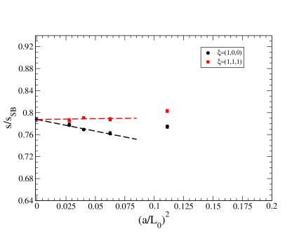
In Fig. 1 we show the results for $\bar{\Sigma}=\Sigma-\Sigma_{0}+1$ as a function of $(a/L_{0})^{2}$ for the 8 highest temperatures, where $(\Sigma_{0}-1)$ are the tree-level discretization effects that are subtracted analytically Giusti and Meyer (2013). The statistical errors range from 1 per-mille up to 3.5 per-mille. For these data sets the residual lattice artifacts turn out to be very small, and at most of $2\%$ already at $L_{0}/a=3$. A continuum linear extrapolation in $(a/L_{0})^{2}$ of the three points with finer lattice spacings works very well for all data sets as shown in Fig. 1. The intercepts of these fits are our best estimate of the step-scaling function in the continuum limit. A quadratic fit of all four points give always compatible results within the statistical errors. The same applies for a combined fit of all data with discretization effects parametrized as expected in the weak coupling expansion. 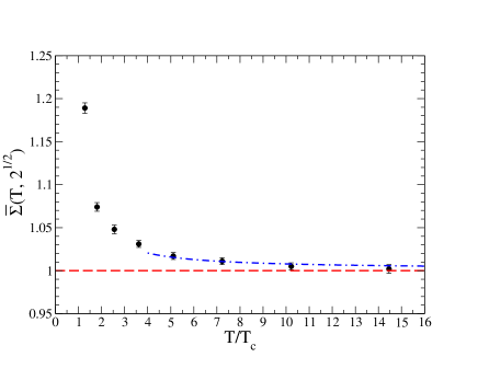For the last 5 temperatures we interpolate the results for $\Sigma_{s}(T,\sqrt{2})$ in the renormalized coupling, and use the fit function to correct for the slight mismatch in the scales from Ref. Capitani et al. (1999). The best values for the step-scaling function are given in Tab. 1, and shown in the left plot of Fig. 2.
The renormalization constant $Z_{T}$ has been determined from Eq. (8). In this case it is not necessary to consider large spatial volumes, and the numerical simulations have been performed with $L/a=12$ and $16$. The finite-volume $\langle T_{0k}\rangle_{\bm{\xi}}$ in the denominator has been computed as described above. The derivative in the numerator requires the calculation of a ratio of two partition functions which cannot be computed in a single Monte Carlo simulation due to the very poor overlap of the relevant phase space of the two integrals. In this case we have used the Monte Carlo procedure of Refs. Giusti and Meyer (2011b); Della Morte and Giusti (2011). We consider a set of $(n+1)$ systems with action $\overline{S}(U,r_{i})=r_{i}S(U^{({\bm{\xi}}-a/L_{0}\hat{k})})+(1-r_{i})S(U^{({\bm{\xi}}+a/L_{0}\hat{k})})$ ($r_{i}=i/n$, $i=0,1,\dots,n$), where the superscript indicates the shift in the boundary conditions. The relevant phase space of two successive systems with $r_{i}$ and $r_{i+1}$ is very similar and the ratio of their partition functions, ${\cal Z}(\beta,r_{i})/{\cal Z}(\beta,r_{i+1})$, can be efficiently measured as the expectation value of the observable $O(U,r_{i+1})=\exp{({\overline{S}}(U,r_{i+1})-{\overline{S}}(U,r_{i}))}$ on the ensemble of gauge configurations generated with the action ${\overline{S}}(U,r_{i+1})$ Della Morte and Giusti (2009). The discrete derivative is then written as

$$\frac{1}{2a}\ln{\frac{Z(L_{0},{\bm{\xi}}+a/L_{0}\hat{k})}{Z(L_{0},{\bm{\xi}}-a/L_{0}\hat{k})}}=\frac{1}{2a}\sum_{i=0}^{n-1}\ln{\frac{{\cal Z}(\beta,r_{i})}{{\cal Z}(\beta,r_{i+1})}}\;.$$ (10)

All the details and the results of the computation of $Z_{T}$ will be presented elsewhere Giusti and pepe . In Tab. 2 we report the values of $Z_{T}$ at the 8 values of $\beta$ needed to renormalize the entropy density at the temperature $T_{0}$ computed with shift ${\bm{\xi}}=(1,0,0)$ and $(1,1,1)$. Albeit with smaller statistical errors, our values are in agreement with those found in Ref. Robaina and Meyer (2013). Also in this case we have subtracted the discretiazion effects of the free theory. In each of the two sets of data we keep $L_{0}$ fixed in physical units, so that residual (small) discretization effects in $Z_{T}$ will be removed in the continuum limit extrapolation of the renormalized entropy density. Discretization effects due to finite volume are negligible within our errors. For completeness, in the same Table we also report the corresponding expectation values of $\langle T_{0k}\rangle_{\bm{\xi}}$ in the large volume which enters Eq. (7). The results for $s(T_{0})/T^{3}_{0}$ as defined in Eq. (7) are shown in the right plot of Fig. 1.

$\beta$	$L_{0}/a$	$\;\;\;\;\;\;\;\langle T_{0k}\rangle_{(1,0,0)}$	$\;\;Z_{T}$
$6.0403$	$3$	$-5.4278(22)\,10^{-3}$	$1.585(6)$
$6.2257$	$4$	$-1.7262(5)\,10^{-3}$	$1.523(6)$
$6.3875$	$5$	$-0.7203(5)\,10^{-3}$	$1.497(4)$
$6.5282$	$6$	$-0.3536(5)\,10^{-3}$	$1.484(6)$
$\beta$	$L_{0}/a$	$\;\;\;\;\;\;\;\langle T_{0k}\rangle_{(1,1,1)}$	$\;\;Z_{T}$
$6.2670$	$3$	$-6.584(11)\,10^{-4}$	$1.528(6)$
$6.4822$	$4$	$-2.187(3)\,10^{-4}$	$1.475(6)$
$6.6575$	$5$	$-0.9251(19)\,10^{-4}$	$1.456(3)$
$6.7981$	$6$	$-0.4524(14)\,10^{-4}$	$1.439(6)$

Table 2: The bare vacuum expectation values of $\langle T_{0k}\rangle_{\bm{\xi}}$ at the reference temperature $T_{0}$ for ${\bm{\xi}}=(1,0,0)$ and $(1,1,1)$. The renormalization constant $Z_{T}$ at the corresponding eight $\beta$ values is also reported.

Figure 2: The step-scaling function (left) and the entropy density normalized to the SB value (right) versus the temperature. The dashed lines (red) are the SB values, while the dotted-dashed lines (blue) are the perturbation theory ones from Ref. Kajantie et al. (2003).

The typical statistical error is just below half a percent, while the largest discretization error is roughly $3\%$. The continuum limit extrapolation of the data with ${\bm{\xi}}=(1,0,0)$ and $(1,1,1)$ at the three finer lattices are in excellent agreement among themselves. A combined extrapolation gives $s(T_{0})/s_{\rm SB}(T_{0})=0.788(4)$ with a $\chi^{2}/{\rm dof}=0.74$, see Tab. 1.
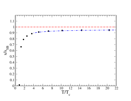
Results and conclusions.— Once the entropy density has been measured at $T_{0}$, $s(T)$ at the other temperatures is computed by solving the straightforward recursive relation for the step-scaling function. The values obtained for the entropy density are reported in Tab. 1 and shown in Fig. 2. The precision reached for $s(T)$ is half a percent at $T_{0}$, and becomes at most $1.5\%$ at $T/T_{0}=8\sqrt{2}$. We expect to reduce the latter error to the same level of the former once the renormalization constant is determined in the full range $0\leq g_{0}^{2}\leq 1$ Giusti and pepe . Taking into account that the entire computation required a few million of core hours on BG/Q, the precision reached shows the potentiality of the strategy.
The results for the entropy density are in agreement with those in Refs. Boyd et al. (1996); Meyer (2009), and for $T>2\,T_{c}$ with the more precise ones in Ref. Borsanyi et al. (2012). Our data differ by several standard deviations from those in Ref. Borsanyi et al. (2012) in the interval $T_{c}<T<2\,T_{c}$. A more detailed comparison will be presented in Ref. Giusti and pepe , where more points will be added in this low-temperature region. The step-scaling function at $T\sim\!15T_{c}$ is already compatible with the high-temperature limit within the half a percent uncertainty quoted. The entropy density, however, still differs from the Stefan-Boltzmann value by rougly $5\%$ at $T\simeq 20\,T_{c}$. To compare with the known perturbative formula Kajantie et al. (2003), we use $\Lambda_{{\overline{\mbox{\scriptsize MS}}}}\,r_{0}=0.586(48)$ Capitani et al. (1999); Necco and Sommer (2002) and we fix the $O(g^{6})$ undetermined coefficient by matching the perturbative value of the entropy density with our data at the largest temperature $T\simeq 20\,T_{c}$. The results are shown in Fig. 2. Despite the good agreement, it must be said that the contribution from the various orders in the perturbative series is oscillating. At our largest temperature the contribution of $O(g^{6})$ is roughly $40\%$ of the total correction to the entropy density given by the other terms, see Ref. Giusti and pepe for more details.
On a more theoretical side, the results presented in this Letter are a direct non-perturbative verification of the consequences of Lorentz invariance at finite T.
Acknowledgments.— We thank H. B. Meyer and D. Robaina for discussions. The simulations were performed on the BG/Q at CINECA (INFN and LISA agreement), and on PC clusters at the Physics Department of the University of Milano-Bicocca. We thankfully acknowledge the computer resources and technical support provided by these institutions. This work was partially supported by the INFN SUMA project.

References

- Boyd et al. (1996) G. Boyd, et al., Nucl.Phys. B469, 419 (1996).
- Borsanyi et al. (2012) S. Borsanyi, et al., JHEP 1207, 056 (2012).
- Cheng et al. (2010) M. Cheng, et al., Phys.Rev. D81, 054504 (2010).
- Borsanyi et al. (2013) S. Borsanyi, et al., (2013), arXiv:1309.5258.
- Philipsen (2013) O. Philipsen, Prog.Part.Nucl.Phys. 70, 55 (2013).
- Giusti and Meyer (2013) L. Giusti and H. B. Meyer, JHEP 1301, 140 (2013).
- Giusti and Meyer (2011a) L. Giusti and H. B. Meyer, JHEP 1111, 087 (2011a).
- Giusti and Meyer (2011b) L. Giusti and H. B. Meyer, Phys.Rev.Lett. 106, 131601 (2011b).
- Della Morte and Giusti (2011) M. Della Morte and L. Giusti, JHEP 1105, 056 (2011).
- Caracciolo et al. (1990) S. Caracciolo, G. Curci, P. Menotti, and A. Pelissetto, Annals Phys. 197, 119 (1990).
- Giusti and Pepe (2013) L. Giusti and M. Pepe, (2013), arXiv:1311.1012.
- Capitani et al. (1999) S. Capitani, M. Luscher, R. Sommer, and H. Wittig (ALPHA Collaboration), Nucl.Phys. B544, 669 (1999).
- Necco and Sommer (2002) S. Necco and R. Sommer, Nucl. Phys. B622, 328 (2002).
- Lucini et al. (2004) B. Lucini, M. Teper, and U. Wenger, JHEP 0401, 061 (2004).
- (15) L. Giusti and M. Pepe, in preparation.
- Della Morte and Giusti (2009) M. Della Morte and L. Giusti, Comput. Phys. Commun. 180, 819 (2009).
- Robaina and Meyer (2013) D. Robaina and H. B. Meyer, (2013), arXiv:1310.6075.
- Meyer (2009) H. B. Meyer, Phys. Rev. D80, 051502 (2009).
- Kajantie et al. (2003) K. Kajantie, M. Laine, K. Rummukainen, and Y. Schroder, Phys.Rev. D67, 105008 (2003).