Testing Composite Hypothesis based on the Density Power Divergence

Basu, A.1; Mandal, A.2; Martin, N.3 and Pardo, L.4
1Indian Statistical Institute, Kolkata 700108, India
2Department of Statistics, University of Pittsburgh, Pittsburgh 15260, USA
3Department of Statistics and O.R. II, Complutense University of Madrid, 28003 Madrid, Spain
4Department of Statistics and O.R. I, Complutense University of Madrid, 28040 Madrid, Spain
Abstract

In any parametric inference problem, the robustness of the procedure is a real concern. A procedure which retains a high degree of efficiency under the model and simultaneously provides stable inference under data contamination is preferable in any practical situation over another procedure which achieves its efficiency at the cost of robustness or vice versa. The density power divergence family of Basu et al. (1998) provides a flexible class of divergences where the adjustment between efficiency and robustness is controlled by a single parameter β𝛽\beta. In this paper we consider general tests of parametric hypotheses based on the density power divergence. We establish the asymptotic null distribution of the test statistic and explore its asymptotic power function. Numerical results illustrate the performance of the theory developed.

AMS 2001 Subject Classification: 62F03, 62F35

keywords and phrases: density power divergence, linear combination of chi-squares, robustness, tests of hypotheses.

1 Introduction

Hypothesis testing is one of the fundamental paradigms of statistical inference. The likelihood ratio test is a key component of the classical theory of hypothesis testing; however, this test is known to be notoriously nonrobust under model misspecification and the presence of outliers. Many density based minimum distance procedures have been observed to have strong robustness properties in estimation and testing together with high efficiency, eg., Pardo (2006) and Basu et al. (2011). Among the available robust tests in the literature, those based on the class of disparities (Simpson, 1989 and Lindsay, 1994) are known to perform well in practical situations and have many theoretical advantages. However the effectiveness of these procedures in continuous models is tempered by the fact that it is necessary to construct a continuous density estimate of the data generating density as an intermediate step. The procedure thus becomes substantially more complicated and loses a part of its appeal. In contrast, none of the density power divergences require any density estimation to implement their minimization routines. Basu et al. (2013) considered parametric hypothesis testing based on the density power divergence for simple null hypotheses. In this paper we extend, in a nontrivial way, the problem for composite null hypotheses in general populations. To do that we have introduced the minimum density power divergence estimator restricted to a general null hypothesis, i.e. the restricted minimum density power divergence estimator. In order to derive the asymptotic distribution of the new family of test statistics proposed in this paper for testing composite null hypotheses, we need the asymptotic distribution of the restricted minimum density power divergence estimator. Thus the theoretical results presented in this paper require a fresh approach and represent a non-trivial generalization of the Basu et al. (2013) paper.

Let {P𝜽:𝜽Θ}conditional-setsubscript𝑃𝜽𝜽Θ\left\{P_{\boldsymbol{\theta}}:\boldsymbol{\theta}\in\Theta\right\} be some identifiable parametric family of probability measures on a measurable space (𝒳(\mathcal{X},𝒜)\mathcal{A)} with an open parameter space Θp,Θsuperscript𝑝\Theta\subset{\mathbb{R}}^{p}, p1.𝑝1p\geq 1. Measures P𝜽subscript𝑃𝜽P_{\boldsymbol{\theta}} are assumed to be described by densities fθ=dPθ/dμsubscript𝑓𝜃𝑑subscript𝑃𝜃𝑑𝜇f_{\theta}=dP_{\theta}/d\mu absolutely continuous with respect to a dominating σ𝜎\sigma-finite measure μ𝜇\mu on 𝒳𝒳\mathcal{X} . Let X1,,Xnsubscript𝑋1subscript𝑋𝑛X_{1},...,X_{n} be a random sample from a density belonging to the family {f𝜽:𝜽Θ}conditional-setsubscript𝑓𝜽𝜽Θ\left\{f_{\boldsymbol{\theta}}:\boldsymbol{\theta}\in\Theta\right\}, where the support of the random variables is independent of the parameter 𝜽𝜽\boldsymbol{\theta}. Consider a general null hypothesis of interest which restricts the parameter to a proper subset Θ0subscriptΘ0\Theta_{0} of ΘΘ\Theta, i.e.

H0:𝜽Θ0againstH1:𝜽Θ0.:subscript𝐻0𝜽subscriptΘ0againstsubscript𝐻1:𝜽subscriptΘ0H_{0}:\boldsymbol{\theta}\in\Theta_{0}~{}\text{against}~{}H_{1}:\boldsymbol{\theta}\notin\Theta_{0}. (1)

In many practical hypothesis testing problems, the restricted parameter space Θ0subscriptΘ0\Theta_{0} is defined by a set of r<p𝑟𝑝r<p restrictions of the form

𝒈(𝜽)=𝟎r𝒈𝜽subscript0𝑟\boldsymbol{g}(\boldsymbol{\theta)=0}_{r} (2)

on ΘΘ\Theta, where 𝒈:pr:𝒈superscript𝑝superscript𝑟\boldsymbol{g}:\mathbb{R}^{p}\rightarrow\mathbb{R}^{r} is a vector-valued function such that the p×r𝑝𝑟p\times r matrix

𝐆(𝜽)=𝒈T(𝜽)𝜽𝐆𝜽superscript𝒈𝑇𝜽𝜽\mathbf{G}\left(\boldsymbol{\theta}\right)=\frac{\partial\boldsymbol{g}^{T}(\boldsymbol{\theta)}}{\partial\boldsymbol{\theta}} (3)

exists and is continuous in 𝜽𝜽\boldsymbol{\theta} and rank(𝐆(𝜽))=r𝐆𝜽𝑟\left(\mathbf{G}\left(\boldsymbol{\theta}\right)\right)=r. Here 𝟎rsubscript0𝑟\boldsymbol{0}_{r} denotes the null vector of dimension r𝑟r, and the superscript T𝑇T in the above represents the transpose of the matrix.

In general, however, there are no uniformly most powerful tests for solving the class of problems formulated in (1). The canonical approaches for problems like these include the likelihood ratio test statistic, the Wald test statistic and the Rao test statistic; see, for instance, Silvey (1975). The tests based on disparities (or divergences), already mentioned earlier, also provide attractive theoretical alternatives for performing the above tests.

In this paper we will solve the hypothesis testing problem presented in (1) using the family of density power divergences. Let 𝒢𝒢\mathcal{G} denote the set of all distributions having densities with respect to the dominating measure. Given any two densities hh and f𝑓f in 𝒢𝒢\mathcal{G}, the density power divergence between them is defined, as the function of a nonnegative tuning parameter β𝛽\beta, as

dβ(h,f)={{f1+β(x)(1+1β)fβ(x)h(x)+1βh1+β(x)}𝑑x,forβ>0,h(x)log(h(x)f(x))𝑑x,forβ=0.subscript𝑑𝛽𝑓casessuperscript𝑓1𝛽𝑥11𝛽superscript𝑓𝛽𝑥𝑥1𝛽superscript1𝛽𝑥differential-d𝑥for𝛽0𝑥𝑥𝑓𝑥differential-d𝑥for𝛽0d_{\beta}(h,f)=\left\{\begin{array}[]{ll}\int\left\{f^{1+\beta}(x)-\left(1+\frac{1}{\beta}\right)f^{\beta}(x)h(x)+\frac{1}{\beta}h^{1+\beta}(x)\right\}dx,&\text{for}\mathrm{~{}}\beta>0,\\[8.61108pt] \int h(x)\log\left(\displaystyle\frac{h(x)}{f(x)}\right)dx,&\text{for}\mathrm{~{}}\beta=0.\end{array}\right. (4)

The case corresponding to β=0𝛽0\beta=0 may be derived from the general case by taking the continuous limit as β0𝛽0\beta\rightarrow 0, and in this case d0(h,f)subscript𝑑0𝑓d_{0}(h,f) is the classical Kullback-Leibler divergence. The quantities defined in equation (4) are genuine divergences in the sense dβ(h,f)0subscript𝑑𝛽𝑓0d_{\beta}(h,f)\geq 0 for all h,f𝒢𝑓𝒢h,f\in\mathcal{G} and all β0𝛽0\beta\geq 0, and dβ(h,f)subscript𝑑𝛽𝑓d_{\beta}(h,f) is equal to zero if and only if the densities hh and f𝑓f are identically equal.

In Section 2 we introduce the restricted minimum density power divergence estimator (RMDPDE); we also study its asymptotic distribution and its relation with the minimum density power divergence estimator (MDPDE) in this section. The new family of test statistics and their asymptotic distributions are presented in Section 3. In Section 4 we describe the relation of the proposed test with the likelihood ratio test for the normal model, and in Section 5 we have considered testing hypotheses for the Weibull model. Numerical results including real data examples are presented in Section 6. The problem of tuning parameter selection is taken up in Section 7. Some concluding remarks are given in Section 8.

In the rest of the paper, we will frequently use the standard assumptions of asymptotic inference as given by Assumptions A, B, C and D of Lehmann (1983, p. 429). We will refer to them as the Lehmann conditions. Some of the proofs will also require the conditions D1–D5 of Basu et al. (2011, p. 304) which we will refer to as Basu et al. conditions. In order to avoid arresting the flow of the paper, these conditions have been presented in the Appendix.

2 Restricted Minimum Density Power Divergence Estimator

We consider the parametric model of densities {f𝜽:𝜽Θp}conditional-setsubscript𝑓𝜽𝜽Θsuperscript𝑝\{f_{\boldsymbol{\theta}}:{\boldsymbol{\theta}}\in\Theta\subset{\mathbb{R}}^{p}\}; suppose that we are interested in the estimation of 𝜽𝜽{{\boldsymbol{\theta}}}. Let H𝐻H represent the distribution function corresponding to the density hh. The minimum density power divergence functional Tβ(H)subscript𝑇𝛽𝐻T_{\beta}(H) at H𝐻H is defined by the requirement dβ(h,fTβ(H))=min𝜽Θdβ(h,f𝜽)subscript𝑑𝛽subscript𝑓subscript𝑇𝛽𝐻subscript𝜽Θsubscript𝑑𝛽subscript𝑓𝜽d_{\beta}(h,f_{T_{\beta}(H)})=\min_{{{\boldsymbol{\theta}}}\in\Theta}d_{\beta}(h,f_{{\boldsymbol{\theta}}}). Clearly the term h1+β(x)𝑑xsuperscript1𝛽𝑥differential-d𝑥\int h^{1+\beta}(x)dx in (4) has no role in the minimization of dβ(h,f𝜽)subscript𝑑𝛽subscript𝑓𝜽d_{\beta}(h,f_{{\boldsymbol{\theta}}}) over 𝜽Θ𝜽Θ{{\boldsymbol{\theta}}}\in\Theta. Thus the essential objective function to be minimized in the computation of the minimum density power divergence functional Tβ(H)subscript𝑇𝛽𝐻T_{\beta}(H) reduces to

{f𝜽1+β(x)(1+1β)f𝜽β(x)h(x)}𝑑x=f𝜽1+β(x)𝑑x(1+1β)f𝜽β(x)𝑑H(x).superscriptsubscript𝑓𝜽1𝛽𝑥11𝛽superscriptsubscript𝑓𝜽𝛽𝑥𝑥differential-d𝑥superscriptsubscript𝑓𝜽1𝛽𝑥differential-d𝑥11𝛽superscriptsubscript𝑓𝜽𝛽𝑥differential-d𝐻𝑥\int\left\{f_{{\boldsymbol{\theta}}}^{1+\beta}(x)-\left(1+\frac{1}{\beta}\right)f_{{\boldsymbol{\theta}}}^{\beta}(x)h(x)\right\}dx=\int f_{{\boldsymbol{\theta}}}^{1+\beta}(x)dx-\left(1+\frac{1}{\beta}\right)\int f_{{\boldsymbol{\theta}}}^{\beta}(x)dH(x). (5)

Notice that in the above objective function the density hh appears only as a linear term (unlike, say, the computation of the of the minimum Hellinger distance functional where the square root of the density hh is the relevant quantity). Thus given a random sample X1,,Xnsubscript𝑋1subscript𝑋𝑛X_{1},\ldots,X_{n} from the distribution H𝐻H we can approximate the above objective function by replacing H𝐻H with its empirical distribution function Hnsubscript𝐻𝑛H_{n}. For a given tuning parameter β𝛽\beta, therefore, the MDPDE 𝜽^βsubscript^𝜽𝛽\widehat{\boldsymbol{\theta}}_{\beta} of 𝜽𝜽{\boldsymbol{\theta}} can be obtained by minimizing

f𝜽1+β(x)𝑑x(1+1β)f𝜽β(x)𝑑Hn(x)superscriptsubscript𝑓𝜽1𝛽𝑥differential-d𝑥11𝛽superscriptsubscript𝑓𝜽𝛽𝑥differential-dsubscript𝐻𝑛𝑥\displaystyle\int f_{{\boldsymbol{\theta}}}^{1+\beta}(x)dx-\left(1+\frac{1}{\beta}\right)\int f_{{\boldsymbol{\theta}}}^{\beta}(x)dH_{n}(x) =f𝜽1+β(x)𝑑x(1+1β)1ni=1nf𝜽β(Xi)absentsuperscriptsubscript𝑓𝜽1𝛽𝑥differential-d𝑥11𝛽1𝑛superscriptsubscript𝑖1𝑛superscriptsubscript𝑓𝜽𝛽subscript𝑋𝑖\displaystyle=\int f_{{\boldsymbol{\theta}}}^{1+\beta}(x)dx-\left(1+\frac{1}{\beta}\right)\frac{1}{n}\sum_{i=1}^{n}f_{{\boldsymbol{\theta}}}^{\beta}(X_{i})
=1ni=1nV𝜽(Xi)absent1𝑛superscriptsubscript𝑖1𝑛subscript𝑉𝜽subscript𝑋𝑖\displaystyle=\frac{1}{n}\sum_{i=1}^{n}V_{\boldsymbol{\theta}}(X_{i}) (6)

over 𝜽Θ𝜽Θ{{\boldsymbol{\theta}}}\in\Theta, where V𝜽(x)=f𝜽1+β(y)𝑑y(1+1β)f𝜽β(x)subscript𝑉𝜽𝑥superscriptsubscript𝑓𝜽1𝛽𝑦differential-d𝑦11𝛽superscriptsubscript𝑓𝜽𝛽𝑥V_{\boldsymbol{\theta}}(x)=\int f_{{\boldsymbol{\theta}}}^{1+\beta}(y)dy-\left(1+\frac{1}{\beta}\right)f_{{\boldsymbol{\theta}}}^{\beta}(x). In the special case β=0𝛽0\beta=0, the objective function reduces to 1ni=1nlogf𝜽(Xi)1𝑛superscriptsubscript𝑖1𝑛subscript𝑓𝜽subscript𝑋𝑖-\frac{1}{n}\sum_{i=1}^{n}\log f_{\boldsymbol{\theta}}(X_{i}); the corresponding minimizer turns out to be the maximum likelihood estimator (MLE) of 𝜽𝜽\boldsymbol{\theta}. The minimization of the expression in (6) over 𝜽𝜽{{\boldsymbol{\theta}}} does not require the use of a nonparametric density estimate of the true unknown distribution H𝐻H. Existing theory (e.g. De Angelis and Young, 1992) shows that in general there is little or no advantage in introducing smoothing for such functionals which may be empirically estimated using the empirical distribution function alone, except in very special cases. Using Hnsubscript𝐻𝑛H_{n} as a substitute for H𝐻H, if possible, is therefore a natural step.

Let 𝒖𝜽(x)=𝜽logf𝜽(x)subscript𝒖𝜽𝑥𝜽subscript𝑓𝜽𝑥\boldsymbol{u}_{{\boldsymbol{\theta}}}(x)=\frac{\partial}{\partial\boldsymbol{\theta}}\log f_{{\boldsymbol{\theta}}}(x) be the likelihood score function of the model. Under differentiability of the model the minimization of the objective function in equation (6) leads to an estimating equation of the form

1ni=1n𝒖𝜽(Xi)f𝜽β(Xi)𝒖𝜽(x)f𝜽1+β(x)𝑑x=𝟎p,1𝑛superscriptsubscript𝑖1𝑛subscript𝒖𝜽subscript𝑋𝑖superscriptsubscript𝑓𝜽𝛽subscript𝑋𝑖subscript𝒖𝜽𝑥superscriptsubscript𝑓𝜽1𝛽𝑥differential-d𝑥subscript0𝑝\frac{1}{n}\sum_{i=1}^{n}\boldsymbol{u}_{{\boldsymbol{\theta}}}(X_{i})f_{{\boldsymbol{\theta}}}^{\beta}(X_{i})-\int\boldsymbol{u}_{{\boldsymbol{\theta}}}(x)f_{{\boldsymbol{\theta}}}^{1+\beta}(x)dx=\boldsymbol{0}_{p}, (7)

which is an unbiased estimating equation under the model. Since the corresponding estimating equation weights the score 𝒖𝜽(Xi)subscript𝒖𝜽subscript𝑋𝑖\boldsymbol{u}_{\boldsymbol{\theta}}(X_{i}) with the power of the density f𝜽β(Xi)superscriptsubscript𝑓𝜽𝛽subscript𝑋𝑖f_{\boldsymbol{\theta}}^{\beta}(X_{i}), the outlier resistant behavior of the estimator is intuitively apparent. See Basu et al. (1998) and Jones et al. (2001) for more details.

The functional Tβ(H)subscript𝑇𝛽𝐻T_{\beta}(H) is Fisher consistent; it takes the value 𝜽0subscript𝜽0\boldsymbol{\theta}_{0} when the true density h=f𝜽0subscript𝑓subscript𝜽0h=f_{\boldsymbol{\theta}_{0}} is in the model. When it is not, 𝜽βh=Tβ(H)superscriptsubscript𝜽𝛽subscript𝑇𝛽𝐻\boldsymbol{\theta}_{\beta}^{h}=T_{\beta}(H) represents the best fitting parameter. For brevity we will suppress the hh superscript in the notation for 𝜽βhsuperscriptsubscript𝜽𝛽\boldsymbol{\theta}_{\beta}^{h}; f𝜽βsubscript𝑓subscript𝜽𝛽f_{\boldsymbol{\theta}_{\beta}} is the model element closest to the density hh in the density power divergence sense corresponding to tuning parameter β𝛽\beta.

Let hh be the true data generating density, and 𝜽β=Tβ(H)subscript𝜽𝛽subscript𝑇𝛽𝐻{\boldsymbol{\theta}}_{\beta}=T_{\beta}(H) be the best fitting parameter. To set up the notation we define the quantities

𝑱β(𝜽)subscript𝑱𝛽𝜽\displaystyle\boldsymbol{J}_{\beta}(\boldsymbol{\theta}) =𝒖𝜽(x)𝒖𝜽T(x)f𝜽1+β(x)𝑑x+{𝑰𝜽(x)β𝒖𝜽(x)𝒖𝜽T(x)}{h(x)f𝜽(x)}f𝜽β(x)𝑑x,absentsubscript𝒖𝜽𝑥superscriptsubscript𝒖𝜽𝑇𝑥superscriptsubscript𝑓𝜽1𝛽𝑥differential-d𝑥subscript𝑰𝜽𝑥𝛽subscript𝒖𝜽𝑥superscriptsubscript𝒖𝜽𝑇𝑥𝑥subscript𝑓𝜽𝑥superscriptsubscript𝑓𝜽𝛽𝑥differential-d𝑥\displaystyle=\int\boldsymbol{u}_{{\boldsymbol{\theta}}}(x)\boldsymbol{u}_{{\boldsymbol{\theta}}}^{T}(x)f_{{\boldsymbol{\theta}}}^{1+\beta}(x)dx+\int\{\boldsymbol{I}_{\boldsymbol{\theta}}(x)-\beta\boldsymbol{u}_{\boldsymbol{\theta}}(x)\boldsymbol{u}_{\boldsymbol{\theta}}^{T}(x)\}\{h(x)-f_{\boldsymbol{\theta}}(x)\}f_{{\boldsymbol{\theta}}}^{\beta}(x)dx, (8)
𝑲β(𝜽)subscript𝑲𝛽𝜽\displaystyle\boldsymbol{K}_{\beta}(\boldsymbol{\theta}) =𝒖𝜽(x)𝒖𝜽T(x)f𝜽2β(x)h(x)𝑑x𝝃β(𝜽)𝝃βT(𝜽),absentsubscript𝒖𝜽𝑥superscriptsubscript𝒖𝜽𝑇𝑥superscriptsubscript𝑓𝜽2𝛽𝑥𝑥differential-d𝑥subscript𝝃𝛽𝜽superscriptsubscript𝝃𝛽𝑇𝜽\displaystyle=\int\boldsymbol{u}_{{\boldsymbol{\theta}}}(x)\boldsymbol{u}_{{\boldsymbol{\theta}}}^{T}(x)f_{{\boldsymbol{\theta}}}^{2\beta}(x)h(x)dx-\boldsymbol{\xi}_{\beta}({{\boldsymbol{\theta}}})\boldsymbol{\xi}_{\beta}^{T}({{\boldsymbol{\theta}}}), (9)

where 𝝃β(𝜽)=𝒖θ(x)f𝜽β(x)h(x)𝑑xsubscript𝝃𝛽𝜽subscript𝒖𝜃𝑥superscriptsubscript𝑓𝜽𝛽𝑥𝑥differential-d𝑥\boldsymbol{\xi}_{\beta}({{\boldsymbol{\theta}}})=\int\boldsymbol{u}_{\mathbf{\theta}}(x)f_{\boldsymbol{\theta}}^{\beta}(x)h(x)dx, and 𝑰𝜽(x)=𝜽𝒖𝜽(x)subscript𝑰𝜽𝑥𝜽subscript𝒖𝜽𝑥\boldsymbol{I}_{\boldsymbol{\theta}}(x)=-\frac{\partial}{\partial\boldsymbol{\theta}}\boldsymbol{u}_{\boldsymbol{\theta}}(x) is the so called information function of the model.

The following results, proved in Basu et al. (2011), form the basis of our subsequent developments.

Theorem 1

We assume that the Basu et al. conditions are true. Then

  1. a)

    The minimum density power divergence estimating equation (7) has a consistent sequence of roots 𝜽^n,βsubscript^𝜽𝑛𝛽\widehat{\boldsymbol{\theta}}_{n,\beta} (denoted, hereafter, as 𝜽^βsubscript^𝜽𝛽\widehat{\boldsymbol{\theta}}_{\beta}), i.e. 𝜽^βn𝒫𝜽βsubscript^𝜽𝛽𝑛𝒫subscript𝜽𝛽\widehat{\boldsymbol{\theta}}_{\beta}\underset{n\rightarrow\infty}{\overset{\mathcal{P}}{\longrightarrow}}\boldsymbol{\theta}_{\beta}.

  2. b)

    n1/2(𝜽^β𝜽β)superscript𝑛12subscript^𝜽𝛽subscript𝜽𝛽n^{1/2}(\widehat{\boldsymbol{\theta}}_{\beta}-{\boldsymbol{\theta}}_{\beta}) has an asymptotic multivariate normal distribution with (vector) mean zero and covariance matrix 𝑱1𝑲𝑱1superscript𝑱1𝑲superscript𝑱1\boldsymbol{J}^{-1}\boldsymbol{K}\boldsymbol{J}^{-1}, where 𝑱=𝑱β(𝜽β)𝑱subscript𝑱𝛽subscript𝜽𝛽\boldsymbol{J}=\boldsymbol{J}_{\beta}({{\boldsymbol{\theta}}}_{\beta}), 𝑲=𝑲β(𝜽β)𝑲subscript𝑲𝛽subscript𝜽𝛽\boldsymbol{K}=\boldsymbol{K}_{\beta}({{\boldsymbol{\theta}}}_{\beta}) are as in (8) and (9) respectively.

The above result is similar, in content and spirit, to those of White (1982). When the true distribution H𝐻H belongs to the model so that H=F𝜽𝐻subscript𝐹𝜽H=F_{\boldsymbol{\theta}} for some 𝜽Θ𝜽Θ\boldsymbol{\theta}\in\Theta, the formula for 𝑱𝑱\boldsymbol{J}, 𝑲𝑲\boldsymbol{K} and 𝝃𝝃\boldsymbol{\xi} simplify to

𝑱𝑱\displaystyle\boldsymbol{J} =𝑱β(𝜽)=𝒖𝜽(x)𝒖𝜽T(x)f𝜽1+β(x)𝑑x,absentsubscript𝑱𝛽𝜽subscript𝒖𝜽𝑥superscriptsubscript𝒖𝜽𝑇𝑥superscriptsubscript𝑓𝜽1𝛽𝑥differential-d𝑥\displaystyle=\boldsymbol{J}_{\beta}(\boldsymbol{\theta})=\int\boldsymbol{u}_{\boldsymbol{\theta}}(x)\boldsymbol{u}_{\boldsymbol{\theta}}^{T}(x)f_{\boldsymbol{\theta}}^{1+\beta}(x)dx, (10)
𝑲𝑲\displaystyle\boldsymbol{K} =𝑲β(𝜽)=𝒖𝜽(x)𝒖𝜽T(x)f𝜽1+2β(x)𝑑x𝝃𝝃T,absentsubscript𝑲𝛽𝜽subscript𝒖𝜽𝑥superscriptsubscript𝒖𝜽𝑇𝑥superscriptsubscript𝑓𝜽12𝛽𝑥differential-d𝑥𝝃superscript𝝃𝑇\displaystyle=\boldsymbol{K}_{\beta}(\boldsymbol{\theta})=\int\boldsymbol{u}_{\boldsymbol{\theta}}(x)\boldsymbol{u}_{\boldsymbol{\theta}}^{T}(x)f_{\boldsymbol{\theta}}^{1+2\beta}(x)dx-\boldsymbol{\xi}\boldsymbol{\xi}^{T}, (11)
𝝃𝝃\displaystyle\boldsymbol{\xi} =𝝃β(𝜽)=𝒖𝜽(x)f𝜽1+β(x)𝑑x.absentsubscript𝝃𝛽𝜽subscript𝒖𝜽𝑥superscriptsubscript𝑓𝜽1𝛽𝑥differential-d𝑥\displaystyle=\boldsymbol{\xi}_{\beta}(\boldsymbol{\theta})=\int\boldsymbol{u}_{\boldsymbol{\theta}}(x)f_{\boldsymbol{\theta}}^{1+\beta}(x)dx.

The restricted minimum density power divergence functional Tβ0(H)superscriptsubscript𝑇𝛽0𝐻T_{\beta}^{0}(H) at H𝐻H, on the other hand, is the value in the parameter space which satisfies

dβ(h,fTβ0(H))=min𝜽Θ0dβ(h,f𝜽),subscript𝑑𝛽subscript𝑓superscriptsubscript𝑇𝛽0𝐻subscript𝜽subscriptΘ0subscript𝑑𝛽subscript𝑓𝜽d_{\beta}(h,f_{T_{\beta}^{0}(H)})=\min_{{{\boldsymbol{\theta}}}\in\Theta_{0}}d_{\beta}(h,f_{{\boldsymbol{\theta}}}),

provided such a minimizer exists. When a random sample X1,,Xnsubscript𝑋1subscript𝑋𝑛X_{1},\ldots,X_{n} is available from the distribution H𝐻H, the restricted minimum density power divergence estimator of 𝜽𝜽\boldsymbol{\theta} minimizes (6) subject to 𝒈(𝜽)=𝟎r𝒈𝜽subscript0𝑟\boldsymbol{g}(\boldsymbol{\theta)=0}_{r}. Under this set up we will determine, in the next theorem, the asymptotic distribution of the restricted minimum density power divergence estimator (RMDPDE) 𝜽~βsubscript~𝜽𝛽\widetilde{\boldsymbol{\theta}}_{\beta} of 𝜽𝜽\boldsymbol{\theta}.

Theorem 2

Assume that the Lehmann and Basu et al. conditions hold. Suppose that the true distribution belongs to the model, and 𝛉0𝚯0subscript𝛉0subscript𝚯0\boldsymbol{\theta}_{0}\in\boldsymbol{\Theta}_{0} is the true parameter. Then the minimum density power divergence estimator 𝛉~βsubscript~𝛉𝛽\widetilde{\boldsymbol{\theta}}_{\beta} of 𝛉𝛉\boldsymbol{\theta} obtained under the constraints 𝐠(𝛉)=𝟎r𝐠𝛉subscript0𝑟\boldsymbol{g}(\boldsymbol{\theta})=\boldsymbol{0}_{r} of the null hypothesis has the distribution

n1/2(𝜽~β𝜽0)n𝒩(𝟎p,𝚺β(𝜽0))superscript𝑛12subscript~𝜽𝛽subscript𝜽0𝑛𝒩subscript0𝑝subscript𝚺𝛽subscript𝜽0n^{1/2}(\widetilde{\boldsymbol{\theta}}_{\beta}-\boldsymbol{\theta}_{0})\underset{n\rightarrow\infty}{\overset{\mathcal{L}}{\longrightarrow}}\mathcal{N}(\boldsymbol{0}_{p},\boldsymbol{\Sigma}_{\beta}(\boldsymbol{\theta}_{0})\boldsymbol{)}

where

𝚺β(𝜽0)=𝑷β(𝜽0)𝑲β(𝜽0)𝑷β(𝜽0),subscript𝚺𝛽subscript𝜽0subscript𝑷𝛽subscript𝜽0subscript𝑲𝛽subscript𝜽0subscript𝑷𝛽subscript𝜽0\boldsymbol{\Sigma}_{\beta}(\boldsymbol{\theta}_{0})=\boldsymbol{P}_{\beta}(\boldsymbol{\theta}_{0})\boldsymbol{K}_{\beta}(\boldsymbol{\theta}_{0})\boldsymbol{P}_{\beta}(\boldsymbol{\theta}_{0}),
𝑷=𝑷β(𝜽0)=𝑱β1(𝜽0)𝑸β(𝜽0)𝑮T(𝜽0)𝑱β1(𝜽0),𝑷subscript𝑷𝛽subscript𝜽0superscriptsubscript𝑱𝛽1subscript𝜽0subscript𝑸𝛽subscript𝜽0superscript𝑮𝑇subscript𝜽0superscriptsubscript𝑱𝛽1subscript𝜽0\boldsymbol{P=P}_{\beta}(\boldsymbol{\theta}_{0})=\boldsymbol{J}_{\beta}^{-1}(\boldsymbol{\theta}_{0})-\boldsymbol{Q}_{\beta}(\boldsymbol{\theta}_{0})\boldsymbol{G}^{T}(\boldsymbol{\theta}_{0})\boldsymbol{J}_{\beta}^{-1}(\boldsymbol{\theta}_{0}), (12)
𝑸=𝑸β(𝜽0)=𝑱β1(𝜽0)𝑮(𝜽0)[𝑮T(𝜽0)𝑱β1(𝜽0)𝑮(𝜽0)]1.𝑸subscript𝑸𝛽subscript𝜽0superscriptsubscript𝑱𝛽1subscript𝜽0𝑮subscript𝜽0superscriptdelimited-[]superscript𝑮𝑇subscript𝜽0superscriptsubscript𝑱𝛽1subscript𝜽0𝑮subscript𝜽01\boldsymbol{Q=Q}_{\beta}(\boldsymbol{\theta}_{0})=\boldsymbol{J}_{\beta}^{-1}(\boldsymbol{\theta}_{0})\boldsymbol{G}(\boldsymbol{\theta}_{0})\left[\boldsymbol{G}^{T}(\boldsymbol{\theta}_{0})\boldsymbol{J}_{\beta}^{-1}(\boldsymbol{\theta}_{0})\boldsymbol{G}(\boldsymbol{\theta}_{0})\right]^{-1}. (13)

and 𝐉β(𝛉0)subscript𝐉𝛽subscript𝛉0\boldsymbol{J}_{\beta}(\boldsymbol{\theta}_{0}) is as defined in (10), evaluated at 𝛉=𝛉0𝛉subscript𝛉0\boldsymbol{\theta}=\boldsymbol{\theta}_{0}.

Proof. See the Appendix.


3 Testing Parametric Composite Hypotheses using Density Power Divergence

Suppose 𝜽^βsubscript^𝜽𝛽\widehat{\boldsymbol{\theta}}_{\beta} is the unconstrained estimator of 𝜽𝜽\boldsymbol{\theta}, whereas 𝜽~βsubscript~𝜽𝛽\widetilde{\boldsymbol{\theta}}_{\beta} is the RMDPDE under the null hypothesis given in (1). In this section we will present the family of the density power divergence test statistics (DPDTS) for testing the composite null hypothesis in (1). This family of test statistics has the expression

T𝜸(𝜽^β,𝜽~β)=2ndγ(f𝜽^β,f𝜽~β),subscript𝑇𝜸subscript^𝜽𝛽subscript~𝜽𝛽2𝑛subscript𝑑𝛾subscript𝑓subscript^𝜽𝛽subscript𝑓subscript~𝜽𝛽T_{\boldsymbol{\gamma}}(\widehat{\boldsymbol{\theta}}_{\beta},\widetilde{\boldsymbol{\theta}}_{\beta})=2nd_{\gamma}(f_{\widehat{\boldsymbol{\theta}}_{\beta}},f_{\widetilde{\boldsymbol{\theta}}_{\beta}}), (14)

where dγ(f𝜽^β,f𝜽~𝜷)subscript𝑑𝛾subscript𝑓subscript^𝜽𝛽subscript𝑓subscript~𝜽𝜷d_{\gamma}(f_{\widehat{\boldsymbol{\theta}}_{\beta}},f_{\widetilde{\boldsymbol{\theta}}_{\boldsymbol{\beta}}}) is given in (4). In the following theorem we present the asymptotic distribution of the family of DPDTS defined in (14).

Theorem 3

Assume that the Lehmann and Basu et al. conditions hold. The asymptotic distribution of T𝛄(𝛉^β,𝛉~β)subscript𝑇𝛄subscript^𝛉𝛽subscript~𝛉𝛽T_{\boldsymbol{\gamma}}(\widehat{\boldsymbol{\theta}}_{\beta},\widetilde{\boldsymbol{\theta}}_{\beta}) defined in (14) coincides, under the null hypothesis H0subscript𝐻0H_{0} given in (1), with the distribution of the random variable

i=1kλiβ,γ(𝜽0)Zi2,superscriptsubscript𝑖1𝑘superscriptsubscript𝜆𝑖𝛽𝛾subscript𝜽0superscriptsubscript𝑍𝑖2{\textstyle\sum\limits_{i=1}^{k}}\lambda_{i}^{\beta,\gamma}(\boldsymbol{\theta}_{0})Z_{i}^{2},

where Z1,,Zksubscript𝑍1subscript𝑍𝑘Z_{1},\ldots,Z_{k} are independent standard normal variables, λ1β,γ(𝛉0),,λkβ,γ(𝛉0)superscriptsubscript𝜆1𝛽𝛾subscript𝛉0superscriptsubscript𝜆𝑘𝛽𝛾subscript𝛉0\lambda_{1}^{\beta,\gamma}(\boldsymbol{\theta}_{0}),\ldots,\lambda_{k}^{\beta,\gamma}(\boldsymbol{\theta}_{0}) are the nonzero eigenvalues of 𝐀γ(𝛉0)𝐁β(𝛉0)𝐊β(𝛉0)𝐁β(𝛉0)subscript𝐀𝛾subscript𝛉0subscript𝐁𝛽subscript𝛉0subscript𝐊𝛽subscript𝛉0subscript𝐁𝛽subscript𝛉0\boldsymbol{A}_{\gamma}\left(\boldsymbol{\theta}_{0}\right)\boldsymbol{B}_{\beta}\left(\boldsymbol{\theta}_{0}\right)\boldsymbol{K}_{\beta}(\boldsymbol{\theta}_{0})\boldsymbol{B}_{\beta}\left(\boldsymbol{\theta}_{0}\right) and

k=rank(𝑩β(𝜽0)𝑲β(𝜽0)𝑩β(𝜽0)𝑨γ(𝜽0)𝑩β(𝜽0)𝑲β(𝜽0)𝑩β(𝜽0)).𝑘𝑟𝑎𝑛𝑘subscript𝑩𝛽subscript𝜽0subscript𝑲𝛽subscript𝜽0subscript𝑩𝛽subscript𝜽0subscript𝑨𝛾subscript𝜽0subscript𝑩𝛽subscript𝜽0subscript𝑲𝛽subscript𝜽0subscript𝑩𝛽subscript𝜽0k=rank\left(\boldsymbol{B}_{\beta}\left(\boldsymbol{\theta}_{0}\right)\boldsymbol{K}_{\beta}(\boldsymbol{\theta}_{0})\boldsymbol{B}_{\beta}\left(\boldsymbol{\theta}_{0}\right)\boldsymbol{A}_{\gamma}\left(\boldsymbol{\theta}_{0}\right)\boldsymbol{B}_{\beta}\left(\boldsymbol{\theta}_{0}\right)\boldsymbol{K}_{\beta}(\boldsymbol{\theta}_{0})\boldsymbol{B}_{\beta}\left(\boldsymbol{\theta}_{0}\right)\right). (15)

The matrices 𝐀γ(𝛉0)subscript𝐀𝛾subscript𝛉0\boldsymbol{A}_{\gamma}\left(\boldsymbol{\theta}_{0}\right) and 𝐁β(𝛉0)subscript𝐁𝛽subscript𝛉0\boldsymbol{B}_{\beta}\left(\boldsymbol{\theta}_{0}\right) are defined by

𝑨γ(𝜽0)=(aijγ(𝜽0))i,j=1,,p=(1+γ)(𝒳f𝜽0γ1(x)f𝜽0(x)θjf𝜽0(x)θi𝑑x)i,j=1,,p,subscript𝑨𝛾subscript𝜽0subscriptsuperscriptsubscript𝑎𝑖𝑗𝛾subscript𝜽0formulae-sequence𝑖𝑗1𝑝1𝛾subscriptsubscript𝒳superscriptsubscript𝑓subscript𝜽0𝛾1𝑥subscript𝑓subscript𝜽0𝑥subscript𝜃𝑗subscript𝑓subscript𝜽0𝑥subscript𝜃𝑖differential-d𝑥formulae-sequence𝑖𝑗1𝑝\boldsymbol{A}_{\gamma}\left(\boldsymbol{\theta}_{0}\right)=\left(a_{ij}^{\gamma}\left(\boldsymbol{\theta}_{0}\right)\right)_{i,j=1,...,p}=\left(1+\gamma\right)\left(\int\nolimits_{\mathcal{X}}f_{\boldsymbol{\theta}_{0}}^{\gamma-1}\left(x\right)\frac{\partial f_{\boldsymbol{\theta}_{0}}\left(x\right)}{\partial\theta_{j}}\frac{\partial f_{\boldsymbol{\theta}_{0}}\left(x\right)}{\partial\theta_{i}}dx\right)_{i,j=1,...,p}, (16)

and

𝑩β(𝜽0)=𝑱β1(𝜽0)𝑮(𝜽0)[𝑮T(𝜽0)𝑱β1(𝜽0)𝑮(𝜽0)]1𝑮T(𝜽0)𝑱β1(𝜽0).subscript𝑩𝛽subscript𝜽0superscriptsubscript𝑱𝛽1subscript𝜽0𝑮subscript𝜽0superscriptdelimited-[]superscript𝑮𝑇subscript𝜽0superscriptsubscript𝑱𝛽1subscript𝜽0𝑮subscript𝜽01superscript𝑮𝑇subscript𝜽0superscriptsubscript𝑱𝛽1subscript𝜽0\boldsymbol{B}_{\beta}\left(\boldsymbol{\theta}_{0}\right)=\boldsymbol{J}_{\beta}^{-1}(\boldsymbol{\theta}_{0})\boldsymbol{G}(\boldsymbol{\theta}_{0})\left[\boldsymbol{G}^{T}(\boldsymbol{\theta}_{0})\boldsymbol{J}_{\beta}^{-1}(\boldsymbol{\theta}_{0})\boldsymbol{G}(\boldsymbol{\theta}_{0})\right]^{-1}\boldsymbol{G}^{T}(\boldsymbol{\theta}_{0})\boldsymbol{J}_{\beta}^{-1}(\boldsymbol{\theta}_{0}). (17)

In the above 𝛉0Θ0subscript𝛉0subscriptΘ0\boldsymbol{\theta}_{0}\in\Theta_{0} represents the true unknown value of 𝛉𝛉\boldsymbol{\theta}.

Proof. See the Appendix.


Remark 4

The main point to note in the above proof is that it is by no means a trivial or simple extension of Theorem 1 of Basu et al. (2013). The proof of the latter theorem simply requires the results involving the unrestricted MDPD estimator which has been very well studied in the literature. In the present scenario, one has to deal with both the restricted and unrestricted MDPD estimators. The random nature of the second argument of the DPD makes the derivations substantially more complicated and entirely different techniques have to be applied to the proof of Theorem 3 in this paper. The restricted MDPD estimator which we have employed here only has a limited presence in the literature. In some sense Theorem 2 may also be considered to be a part of Theorem 3, but here we have presented them separately for pedagogical reasons as well as to keep a clear focus in our presentations.

Remark 5

We observe that the ranks of the matrices 𝐁β(𝛉0)𝐊β(𝛉0)𝐁β(𝛉0)subscript𝐁𝛽subscript𝛉0subscript𝐊𝛽subscript𝛉0subscript𝐁𝛽subscript𝛉0\boldsymbol{B}_{\beta}\left(\boldsymbol{\theta}_{0}\right)\boldsymbol{K}_{\beta}(\boldsymbol{\theta}_{0})\boldsymbol{B}_{\beta}\left(\boldsymbol{\theta}_{0}\right) and 𝐁β(𝛉0)𝐊β(𝛉0)𝐁β(𝛉0)𝐀γ(𝛉0)𝐁β(𝛉0)𝐊β(𝛉0)𝐁β(𝛉0)subscript𝐁𝛽subscript𝛉0subscript𝐊𝛽subscript𝛉0subscript𝐁𝛽subscript𝛉0subscript𝐀𝛾subscript𝛉0subscript𝐁𝛽subscript𝛉0subscript𝐊𝛽subscript𝛉0subscript𝐁𝛽subscript𝛉0\boldsymbol{B}_{\beta}\left(\boldsymbol{\theta}_{0}\right)\boldsymbol{K}_{\beta}(\boldsymbol{\theta}_{0})\boldsymbol{B}_{\beta}\left(\boldsymbol{\theta}_{0}\right)\boldsymbol{A}_{\gamma}\left(\boldsymbol{\theta}_{0}\right)\boldsymbol{B}_{\beta}\left(\boldsymbol{\theta}_{0}\right)\boldsymbol{K}_{\beta}(\boldsymbol{\theta}_{0})\boldsymbol{B}_{\beta}\left(\boldsymbol{\theta}_{0}\right) are equal. Moreover, it can be easily shown that rank(𝐁β(𝛉0)𝐊β(𝛉0)𝐁β(𝛉0))=rank(𝐆(𝛉0))=r𝑟𝑎𝑛𝑘subscript𝐁𝛽subscript𝛉0subscript𝐊𝛽subscript𝛉0subscript𝐁𝛽subscript𝛉0𝑟𝑎𝑛𝑘𝐆subscript𝛉0𝑟rank\left(\boldsymbol{B}_{\beta}\left(\boldsymbol{\theta}_{0}\right)\boldsymbol{K}_{\beta}(\boldsymbol{\theta}_{0})\boldsymbol{B}_{\beta}\left(\boldsymbol{\theta}_{0}\right)\right)=rank(\boldsymbol{G}(\boldsymbol{\theta}_{0}))=r. So k=r𝑘𝑟k=r, i.e. there will be exactly r𝑟r non-zero eigenvalues.

Corollary 6

For the special case when we test the null hypothesis H0:μ=μ0:subscript𝐻0𝜇subscript𝜇0H_{0}:\mu=\mu_{0} against H1:μμ0:subscript𝐻1𝜇subscript𝜇0H_{1}:\mu\neq\mu_{0} under the 𝒩(μ,σ2)𝒩𝜇superscript𝜎2\mathcal{N}(\mu,\sigma^{2}) model with σ2superscript𝜎2\sigma^{2} unknown, the matrix 𝐀γ(𝛉0)𝐁β(𝛉0)𝐊β(𝛉0)𝐁β(𝛉0)subscript𝐀𝛾subscript𝛉0subscript𝐁𝛽subscript𝛉0subscript𝐊𝛽subscript𝛉0subscript𝐁𝛽subscript𝛉0\boldsymbol{A}_{\gamma}\left(\boldsymbol{\theta}_{0}\right)\boldsymbol{B}_{\beta}\left(\boldsymbol{\theta}_{0}\right)\boldsymbol{K}_{\beta}(\boldsymbol{\theta}_{0})\boldsymbol{B}_{\beta}\left(\boldsymbol{\theta}_{0}\right) has the form

𝑨γ(𝜽0)𝑩β(𝜽0)𝑲β(𝜽0)𝑩β(𝜽0)=(1σγ(β+1)3γ+1(2β+1)3/2(2π)γ/2000),subscript𝑨𝛾subscript𝜽0subscript𝑩𝛽subscript𝜽0subscript𝑲𝛽subscript𝜽0subscript𝑩𝛽subscript𝜽01superscript𝜎𝛾superscript𝛽13𝛾1superscript2𝛽132superscript2𝜋𝛾2000\boldsymbol{A}_{\gamma}\left(\boldsymbol{\theta}_{0}\right)\boldsymbol{B}_{\beta}\left(\boldsymbol{\theta}_{0}\right)\boldsymbol{K}_{\beta}(\boldsymbol{\theta}_{0})\boldsymbol{B}_{\beta}\left(\boldsymbol{\theta}_{0}\right)=\left(\begin{array}[]{cc}\displaystyle\frac{1}{\sigma^{\gamma}}\frac{(\beta+1)^{3}}{\sqrt{\gamma+1}(2\beta+1)^{3/2}(2\pi)^{\gamma/2}}&0\\ 0&0\end{array}\right),

so that the DPDTS T𝛄(𝛉^β,𝛉~β)=2ndγ(f𝛉^β,f𝛉~β)subscript𝑇𝛄subscript^𝛉𝛽subscript~𝛉𝛽2𝑛subscript𝑑𝛾subscript𝑓subscript^𝛉𝛽subscript𝑓subscript~𝛉𝛽T_{\boldsymbol{\gamma}}(\widehat{\boldsymbol{\theta}}_{\beta},\widetilde{\boldsymbol{\theta}}_{\beta})=2nd_{\gamma}(f_{\widehat{\boldsymbol{\theta}}_{\beta}},f_{\widetilde{\boldsymbol{\theta}}_{\beta}}) has the same asymptotic distribution as that of λ1χ2(1)subscript𝜆1superscript𝜒21\lambda_{1}\chi^{2}(1), where λ1subscript𝜆1\lambda_{1} is the only nonzero eigenvalue of the above matrix (equal to its (1,1)11(1,1)th element). In particular when γ=0𝛾0\gamma=0 and β=0𝛽0\beta=0, this eigenvalue becomes one, so that the DPDTS

Tγ=0(𝜽^β=0,𝜽~β=0)=2ndγ=0(f𝜽^β=0,f𝜽~β=0)subscript𝑇𝛾0subscript^𝜽𝛽0subscript~𝜽𝛽02𝑛subscript𝑑𝛾0subscript𝑓subscript^𝜽𝛽0subscript𝑓subscript~𝜽𝛽0T_{\gamma=0}(\hat{\boldsymbol{\theta}}_{\beta=0},\tilde{\boldsymbol{\theta}}_{\beta=0})=2nd_{\gamma=0}\left(f_{\hat{\boldsymbol{\theta}}_{\beta=0}},f_{\tilde{\boldsymbol{\theta}}_{\beta=0}}\right) (18)

has a simple asymptotic χ2(1)superscript𝜒21\chi^{2}(1) distribution. We will revisit this problem again in Section 4.

A simple approach to approximate the critical region of the DPDTS and perform the test could be the following. The k𝑘k eigenvalues described in Theorem 3 can be expressed as a function of the parameter 𝜽0subscript𝜽0\boldsymbol{\theta}_{0}. Under the null they can be consistently estimated by replacing 𝜽~βsubscript~𝜽𝛽\widetilde{\boldsymbol{\theta}}_{\beta} in place of 𝜽0subscript𝜽0\boldsymbol{\theta}_{0}. Let λ^1,λ^2,,λ^ksubscript^𝜆1subscript^𝜆2subscript^𝜆𝑘\hat{\lambda}_{1},\hat{\lambda}_{2},\cdots,\hat{\lambda}_{k} represent the corresponding estimated eigenvalues. Generating independent observations Z1,Z2,,Zksubscript𝑍1subscript𝑍2subscript𝑍𝑘Z_{1},Z_{2},\cdots,Z_{k} from the N(0,1)𝑁01N(0,1) distribution repeatedly, one can estimate the quantiles of the distribution of i=1kλ^iZi2superscriptsubscript𝑖1𝑘subscript^𝜆𝑖superscriptsubscript𝑍𝑖2\sum_{i=1}^{k}\hat{\lambda}_{i}Z_{i}^{2}, where λ^isubscript^𝜆𝑖\hat{\lambda}_{i}’s are kept fixed during this exercise. The quantiles are then consistent approximations of the true quantiles of the asymptotic null distribution of the statistic in Theorem 3; the experimenter can then perform the test based on the critical values thus obtained. In particular when k=1𝑘1k=1 one can perform the test by comparing Tγ(𝜽^β,𝜽~β)/λ^1subscript𝑇𝛾subscript^𝜽𝛽subscript~𝜽𝛽subscript^𝜆1T_{\gamma}(\widehat{\boldsymbol{\theta}}_{\beta},\widetilde{\boldsymbol{\theta}}_{\beta})/\hat{\lambda}_{1} with the appropriate upper quantile of χ2(1)superscript𝜒21\chi^{2}(1) distribution. Tables of the cumulative distribution of i=1kciZi2superscriptsubscript𝑖1𝑘subscript𝑐𝑖superscriptsubscript𝑍𝑖2{\sum\limits_{i=1}^{k}}c_{i}Z_{i}^{2} are also available in Solomon (1960), Johnson and Kotz (1968), Eckler (1969) and Gupta (1963), which may be helpful in performing the test. Davies (1980) has proposed an algorithm to calculate the critical region corresponding to a linear combination of χ2superscript𝜒2\chi^{2} random variables. Several other conservative approximations of the critical value of the DPDTS are provided in Basu et al. (2013).

3.1 The Power Function

By Theorem 3 the null hypothesis should be rejected if Tγ(𝜽^β,𝜽~β)cαβ,γ,subscript𝑇𝛾subscript^𝜽𝛽subscript~𝜽𝛽superscriptsubscript𝑐𝛼𝛽𝛾T_{\gamma}(\widehat{\boldsymbol{\theta}}_{\beta},\widetilde{\boldsymbol{\theta}}_{\beta})\geq c_{\alpha}^{\beta,\gamma}, where cαβ,γ,superscriptsubscript𝑐𝛼𝛽𝛾c_{\alpha}^{\beta,\gamma,} is the quantile of order (1α)1𝛼(1-\alpha) of the asymptotic distribution of Tγ(𝜽^β,𝜽~β)subscript𝑇𝛾subscript^𝜽𝛽subscript~𝜽𝛽T_{\gamma}(\widehat{\boldsymbol{\theta}}_{\beta},\widetilde{\boldsymbol{\theta}}_{\beta}) under H0subscript𝐻0H_{0}. The following theorem can be used to approximate the power function.

Theorem 7

Suppose Lehmann and Basu et al. conditions are satisfied. Assume that 𝛉Θ0𝛉subscriptΘ0\boldsymbol{\theta}\notin\Theta_{0} is the true value of the parameter such that 𝛉^βn𝑝𝛉subscript^𝛉𝛽𝑝𝑛𝛉\widehat{\boldsymbol{\theta}}_{\beta}\overset{p}{\underset{n\rightarrow\infty}{\longrightarrow}}\boldsymbol{\theta} under H1subscript𝐻1H_{1}. Suppose there exists 𝛉Θ0superscript𝛉subscriptΘ0\boldsymbol{\theta}^{*}\in\Theta_{0} such that the RMDPDE 𝛉~βsubscript~𝛉𝛽\widetilde{\boldsymbol{\theta}}_{\beta} of 𝛉𝛉\boldsymbol{\theta} satisfies 𝛉~βn𝑝𝛉subscript~𝛉𝛽𝑝𝑛superscript𝛉\widetilde{\boldsymbol{\theta}}_{\beta}\overset{p}{\underset{n\rightarrow\infty}{\longrightarrow}}\boldsymbol{\theta}^{*}. Further assume that

n1/2((𝜽^β,𝜽~β)(𝜽,𝜽))Tn𝒩((𝟎p𝟎p),(𝑱β1(𝜽)𝑲β(𝜽)𝑱β1(𝜽)𝑨12(𝜽,𝜽)𝑨12(𝜽,𝜽)T𝚺(𝜽,𝜽))),superscript𝑛12superscriptsubscript^𝜽𝛽subscript~𝜽𝛽𝜽superscript𝜽𝑇𝑛𝒩subscript0𝑝subscript0𝑝superscriptsubscript𝑱𝛽1𝜽subscript𝑲𝛽𝜽superscriptsubscript𝑱𝛽1𝜽subscript𝑨12𝜽superscript𝜽subscript𝑨12superscript𝜽superscript𝜽𝑇𝚺𝜽superscript𝜽n^{1/2}\left((\widehat{\boldsymbol{\theta}}_{\beta},\widetilde{\boldsymbol{\theta}}_{\beta})-\left(\boldsymbol{\theta},\boldsymbol{\theta}^{*}\right)\right)^{T}\overset{\mathcal{L}}{\underset{n\rightarrow\infty}{\longrightarrow}}\mathcal{N}\left(\left(\begin{array}[]{l}\boldsymbol{0}_{p}\\ \boldsymbol{0}_{p}\end{array}\right),\left(\begin{array}[]{ll}\boldsymbol{J}_{\beta}^{-1}(\boldsymbol{\theta})\boldsymbol{K}_{\beta}(\boldsymbol{\theta})\boldsymbol{J}_{\beta}^{-1}(\boldsymbol{\theta})&{\boldsymbol{A}}_{12}\left(\boldsymbol{\theta},\boldsymbol{\theta}^{*}\right)\\ {\boldsymbol{A}}_{12}\left(\boldsymbol{\theta},\boldsymbol{\theta}^{*}\right)^{T}&\boldsymbol{\Sigma}\left(\boldsymbol{\theta},\boldsymbol{\theta}^{*}\right)\end{array}\right)\right), (19)

where 𝐀12(𝛉,𝛉)subscript𝐀12𝛉superscript𝛉{\boldsymbol{A}}_{12}\left(\boldsymbol{\theta},\boldsymbol{\theta}^{*}\right) and 𝚺(𝛉,𝛉)𝚺superscript𝛉𝛉\boldsymbol{\Sigma}\left(\boldsymbol{\theta}^{*},\boldsymbol{\theta}\right) are appropriate p×p𝑝𝑝p\times p matrices. Then, under H1subscript𝐻1H_{1}, we have the following convergence

n1/2(dγ(f𝜽^β,f𝜽~β)dγ(f𝜽,f𝜽))n𝐿𝒩(0,σβ,γ2(𝜽,𝜽)),superscript𝑛12subscript𝑑𝛾subscript𝑓subscript^𝜽𝛽subscript𝑓subscript~𝜽𝛽subscript𝑑𝛾subscript𝑓𝜽subscript𝑓superscript𝜽𝐿𝑛𝒩0superscriptsubscript𝜎𝛽𝛾2𝜽superscript𝜽n^{1/2}\left(d_{\gamma}(f_{\widehat{\boldsymbol{\theta}}_{\beta}},f_{\widetilde{\boldsymbol{\theta}}_{\beta}})-d_{\gamma}(f_{\boldsymbol{\theta}},f_{\boldsymbol{\theta}^{*}})\right)\overset{L}{\underset{n\rightarrow\infty}{\longrightarrow}}\mathcal{N}\left(0,\sigma_{\beta,\gamma}^{2}\left(\mathbf{\boldsymbol{\theta}},\boldsymbol{\theta}^{*}\right)\right),

where

σβ,γ2(𝜽,𝜽0)=𝒕T𝑱β1(𝜽)𝑲β(𝜽)𝑱β1(𝜽)𝒕+2𝒕T𝑨12(𝜽,𝜽)𝒔+𝒔T𝚺(𝜽,𝜽)𝒔,superscriptsubscript𝜎𝛽𝛾2𝜽subscript𝜽0superscript𝒕𝑇superscriptsubscript𝑱𝛽1𝜽subscript𝑲𝛽𝜽superscriptsubscript𝑱𝛽1𝜽𝒕2superscript𝒕𝑇subscript𝑨12𝜽superscript𝜽𝒔superscript𝒔𝑇𝚺𝜽superscript𝜽𝒔\sigma_{\beta,\gamma}^{2}\left(\mathbf{\boldsymbol{\theta}},\boldsymbol{\theta}_{0}\right)=\boldsymbol{t}^{T}\boldsymbol{J}_{\beta}^{-1}(\boldsymbol{\theta})\boldsymbol{K}_{\beta}(\boldsymbol{\theta})\boldsymbol{J}_{\beta}^{-1}(\boldsymbol{\theta})\boldsymbol{t+}2\boldsymbol{t}^{T}\boldsymbol{A}_{12}\left(\boldsymbol{\theta},\boldsymbol{\theta}^{*}\right)\boldsymbol{s+s}^{T}\boldsymbol{\Sigma}\left(\boldsymbol{\theta},\boldsymbol{\theta}^{*}\right)\boldsymbol{s}, (20)

and

𝒕=(dγ(f𝜽1,f𝜽)𝜽1)𝜽1=𝜽 and 𝒔=(dγ(f𝜽,f𝜽2)𝜽2)𝜽2=𝜽.𝒕subscriptsubscript𝑑𝛾subscript𝑓subscript𝜽1subscript𝑓superscript𝜽subscript𝜽1subscript𝜽1𝜽 and 𝒔subscriptsubscript𝑑𝛾subscript𝑓𝜽subscript𝑓subscript𝜽2subscript𝜽2subscript𝜽2superscript𝜽\boldsymbol{t=}\left(\frac{\partial d_{\gamma}(f_{\boldsymbol{\theta}_{1}},f_{\boldsymbol{\theta}^{*}})}{\partial\boldsymbol{\theta}_{1}}\right)_{\boldsymbol{\theta}_{1}=\mathbf{\boldsymbol{\theta}}}\text{ and }\boldsymbol{s=}\left(\frac{\partial d_{\gamma}(f_{\mathbf{\boldsymbol{\theta}}},f_{\boldsymbol{\theta}_{2}})}{\partial\boldsymbol{\theta}_{2}}\right)_{\boldsymbol{\theta}_{2}=\mathbf{\boldsymbol{\theta}}^{*}}.

Proof. The result follows in a straightforward manner by considering a first order Taylor expansion of dγ(f𝜽^β,f𝜽~β)subscript𝑑𝛾subscript𝑓subscript^𝜽𝛽subscript𝑓subscript~𝜽𝛽d_{\gamma}(f_{\widehat{\boldsymbol{\theta}}_{\beta}},f_{\widetilde{\boldsymbol{\theta}}_{\beta}}), which yields

dγ(f𝜽^β,f𝜽~β)=dγ(f𝜽,f𝜽)+𝒕T(𝜽^β𝜽)+𝒔T(𝜽~β𝜽)+o(𝜽^β𝜽+𝜽~β𝜽).subscript𝑑𝛾subscript𝑓subscript^𝜽𝛽subscript𝑓subscript~𝜽𝛽subscript𝑑𝛾subscript𝑓𝜽subscript𝑓superscript𝜽superscript𝒕𝑇subscript^𝜽𝛽𝜽superscript𝒔𝑇subscript~𝜽𝛽superscript𝜽𝑜normsubscript^𝜽𝛽𝜽normsubscript~𝜽𝛽superscript𝜽d_{\gamma}(f_{\widehat{\boldsymbol{\theta}}_{\beta}},f_{\widetilde{\boldsymbol{\theta}}_{\beta}})=d_{\gamma}(f_{\boldsymbol{\theta}},f_{\boldsymbol{\theta}^{*}})+\boldsymbol{t}^{T}(\widehat{\boldsymbol{\theta}}_{\beta}-\boldsymbol{\theta})+\boldsymbol{s}^{T}(\widetilde{\boldsymbol{\theta}}_{\beta}-\boldsymbol{\theta}^{*})+o\left(\left\|\widehat{\boldsymbol{\theta}}_{\beta}-\boldsymbol{\theta}\right\|+\left\|\widetilde{\boldsymbol{\theta}}_{\beta}-\boldsymbol{\theta}^{*}\right\|\right).


Remark 8

On the basis of the previous theorem we get an approximation of the power function as

πn,αβ,γ(𝜽)superscriptsubscript𝜋𝑛𝛼𝛽𝛾𝜽\displaystyle\pi_{n,\alpha}^{\beta,\gamma}\left(\mathbf{\boldsymbol{\theta}}\right) =\displaystyle= P𝜽(Tγ(𝜽^β,𝜽~β)cαβ,γ)subscriptP𝜽subscript𝑇𝛾subscript^𝜽𝛽subscript~𝜽𝛽superscriptsubscript𝑐𝛼𝛽𝛾\displaystyle\text{P}_{\mathbf{\boldsymbol{\theta}}}\left(T_{\gamma}(\widehat{\boldsymbol{\theta}}_{\beta},\widetilde{\boldsymbol{\theta}}_{\beta})\geq c_{\alpha}^{\beta,\gamma}\right) (21)
=\displaystyle= 1Φ(n1/2σβ,γ(𝜽,𝜽)(cαβ,γ2ndγ(f𝜽,f𝜽))),1Φsuperscript𝑛12subscript𝜎𝛽𝛾𝜽superscript𝜽superscriptsubscript𝑐𝛼𝛽𝛾2𝑛subscript𝑑𝛾subscript𝑓𝜽subscript𝑓superscript𝜽\displaystyle 1-\Phi\left(\frac{n^{1/2}}{\sigma_{\beta,\gamma}\left(\mathbf{\boldsymbol{\theta}},\boldsymbol{\theta}^{*}\right)}\left(\frac{c_{\alpha}^{\beta,\gamma}}{2n}-d_{\gamma}(f_{\boldsymbol{\theta}},f_{\boldsymbol{\theta}^{*}})\right)\right),

where Φ()Φ\Phi(\cdot) is the standard normal distribution function, cαβ,γsuperscriptsubscript𝑐𝛼𝛽𝛾c_{\alpha}^{\beta,\gamma} is the quantile of order 1α1𝛼1-\alpha of the asymptotic distribution of Tγ(𝛉^β,𝛉~β)subscript𝑇𝛾subscript^𝛉𝛽subscript~𝛉𝛽T_{\gamma}(\widehat{\boldsymbol{\theta}}_{\beta},\widetilde{\boldsymbol{\theta}}_{\beta}) under the null hypothesis, and σβ,γ2(𝛉,𝛉)superscriptsubscript𝜎𝛽𝛾2𝛉superscript𝛉\sigma_{\beta,\gamma}^{2}\left(\mathbf{\boldsymbol{\theta}},\boldsymbol{\theta}^{*}\right) is as defined in (20).

If some 𝛉𝛉\mathbf{\boldsymbol{\theta}} 𝛉absentsuperscript𝛉\neq\boldsymbol{\theta}^{*} is the true parameter, then the probability of rejecting H0subscript𝐻0H_{0} for a fixed size α𝛼\alpha tends to one as n𝑛n\rightarrow\infty. So the test statistic is consistent in the Fraser’s (1957) sense.

Obtaining the approximate sample size n𝑛n to guarantee a power of π𝜋\pi at a given alternative 𝛉𝛉\mathbf{\boldsymbol{\theta}} is an interesting application of formula (21). Let n𝑛n be the positive root of the equation

π=1Φ(n1/2σβ,γ(𝜽,𝜽)(cαβ,γ2ndγ(f𝜽,f𝜽))),𝜋1Φsuperscript𝑛12subscript𝜎𝛽𝛾𝜽superscript𝜽superscriptsubscript𝑐𝛼𝛽𝛾2𝑛subscript𝑑𝛾subscript𝑓𝜽subscript𝑓superscript𝜽\pi=1-\Phi\left(\frac{n^{1/2}}{\sigma_{\beta,\gamma}\left(\mathbf{\boldsymbol{\theta}},\boldsymbol{\theta}^{*}\right)}\left(\frac{c_{\alpha}^{\beta,\gamma}}{2n}-d_{\gamma}(f_{\boldsymbol{\theta}},f_{\boldsymbol{\theta}^{*}})\right)\right),

i.e.

n=A+B+A(A+2B)2dγ(f𝜽,f𝜽)2,𝑛𝐴𝐵𝐴𝐴2𝐵2subscript𝑑𝛾superscriptsubscript𝑓𝜽subscript𝑓superscript𝜽2n=\frac{A+B+\sqrt{A(A+2B)}}{2d_{\gamma}(f_{\boldsymbol{\theta}},f_{\boldsymbol{\theta}^{*}})^{2}},

where

A=σβ,γ2(𝜽,𝜽)(Φ1(1π))2,𝐴superscriptsubscript𝜎𝛽𝛾2𝜽superscript𝜽superscriptsuperscriptΦ11𝜋2A=\sigma_{\beta,\gamma}^{2}\left(\mathbf{\boldsymbol{\theta}},\boldsymbol{\theta}^{*}\right)\left(\Phi^{-1}\left(1-\pi\right)\right)^{2},

and B=cαβ,γdγ(f𝛉,f𝛉).𝐵superscriptsubscript𝑐𝛼𝛽𝛾subscript𝑑𝛾subscript𝑓𝛉subscript𝑓superscript𝛉B=c_{\alpha}^{\beta,\gamma}d_{\gamma}(f_{\boldsymbol{\theta}},f_{\boldsymbol{\theta}^{*}}). Then the required sample size is n=[n]+1,𝑛delimited-[]𝑛1n=\left[n\right]+1, where []delimited-[]\left[\cdot\right] is used to denote “integer part of”.

We may also find an alternative approximation of the power of Tγ(𝜽^β,𝜽~β)subscript𝑇𝛾subscript^𝜽𝛽subscript~𝜽𝛽T_{\gamma}(\widehat{\boldsymbol{\theta}}_{\beta},\widetilde{\boldsymbol{\theta}}_{\beta}) at an alternative close to the null hypothesis. Let 𝜽nΘΘ0subscript𝜽𝑛ΘsubscriptΘ0\boldsymbol{\theta}_{n}\in\Theta-\Theta_{0} be a given sequence of alternatives, and let 𝜽0subscript𝜽0\boldsymbol{\theta}_{0} be the element in Θ0subscriptΘ0\Theta_{0} closest to 𝜽nsubscript𝜽𝑛\boldsymbol{\theta}_{n} in the Euclidean distance sense. One possibility to introduce contiguous alternative hypotheses is to consider a fixed 𝒅p𝒅superscript𝑝\boldsymbol{d}\in\mathbb{R}^{p} and to permit 𝜽nsubscript𝜽𝑛\boldsymbol{\theta}_{n} to move towards 𝜽0subscript𝜽0\boldsymbol{\theta}_{0} as n𝑛n increases in the manner specified by the hypothesis

H1,n:𝜽n=𝜽0+n1/2𝒅.:subscript𝐻1𝑛subscript𝜽𝑛subscript𝜽0superscript𝑛12𝒅H_{1,n}:\boldsymbol{\theta}_{n}=\boldsymbol{\theta}_{0}+n^{-1/2}\boldsymbol{d}. (22)
Theorem 9

Suppose that the model satisfies the Lehmann and Basu et al. conditions. Under the contiguous alternative hypotheses H1,nsubscript𝐻1𝑛H_{1,n} given in (22), the asymptotic distribution of Tγ(𝛉^β,𝛉~β)subscript𝑇𝛾subscript^𝛉𝛽subscript~𝛉𝛽T_{\gamma}(\widehat{\boldsymbol{\theta}}_{\beta},\widetilde{\boldsymbol{\theta}}_{\beta}) coincides with the distribution of

i=1kλiβ,γ(𝜽0)(Zi+wi)2+η,superscriptsubscript𝑖1𝑘superscriptsubscript𝜆𝑖𝛽𝛾subscript𝜽0superscriptsubscript𝑍𝑖subscript𝑤𝑖2𝜂{\sum\limits_{i=1}^{k}}\lambda_{i}^{\beta,\gamma}(\boldsymbol{\theta}_{0})\left(Z_{i}+w_{i}\right)^{2}+\eta,

where Z1,,Zrsubscript𝑍1subscript𝑍𝑟Z_{1},\ldots,Z_{r} are independent standard normal variables, λ1β,γ(𝛉0),,λkβ,γ(𝛉0)superscriptsubscript𝜆1𝛽𝛾subscript𝛉0superscriptsubscript𝜆𝑘𝛽𝛾subscript𝛉0\lambda_{1}^{\beta,\gamma}(\boldsymbol{\theta}_{0}),\ldots,\lambda_{k}^{\beta,\gamma}(\boldsymbol{\theta}_{0}) are the positive eigenvalues of 𝐀γ(𝛉0)𝐁β(𝛉0)𝐊β(𝛉0)𝐁β(𝛉0)subscript𝐀𝛾subscript𝛉0subscript𝐁𝛽subscript𝛉0subscript𝐊𝛽subscript𝛉0subscript𝐁𝛽subscript𝛉0\boldsymbol{A}_{\gamma}\left(\boldsymbol{\theta}_{0}\right)\boldsymbol{B}_{\beta}\left(\boldsymbol{\theta}_{0}\right)\boldsymbol{K}_{\beta}(\boldsymbol{\theta}_{0})\boldsymbol{B}_{\beta}\left(\boldsymbol{\theta}_{0}\right), and the values of 𝐰=(w1,,wk)T𝐰superscriptsubscript𝑤1subscript𝑤𝑘𝑇\boldsymbol{w=}\left(w_{1},\ldots,w_{k}\right)^{T} and η𝜂\eta are given by

𝒘=𝚲k1𝑽T𝑺T𝑨γ(𝜽0)𝑩(𝜽𝟎)𝑱𝜷(𝜽𝟎)𝒅,η=(𝑩(𝜽0)𝑱𝒅)T𝑨γ(𝜽0)𝑩(𝜽𝟎)𝑱𝜷(𝜽𝟎)𝒅𝒘T𝚲k𝒘.formulae-sequence𝒘superscriptsubscript𝚲𝑘1superscript𝑽𝑇superscript𝑺𝑇subscript𝑨𝛾subscript𝜽0𝑩subscript𝜽0subscript𝑱𝜷subscript𝜽0𝒅𝜂superscript𝑩subscript𝜽0𝑱𝒅𝑇subscript𝑨𝛾subscript𝜽0𝑩subscript𝜽0subscript𝑱𝜷subscript𝜽0𝒅superscript𝒘𝑇subscript𝚲𝑘𝒘\boldsymbol{w}=\boldsymbol{\Lambda}_{k}^{-1}\boldsymbol{V}^{T}\boldsymbol{S}^{T}\boldsymbol{A}_{\gamma}(\boldsymbol{\theta}_{0})\boldsymbol{B(\boldsymbol{\theta}_{0})\boldsymbol{J}_{\beta}(\boldsymbol{\theta}_{0})d},~{}~{}\eta=\left(\boldsymbol{B}(\boldsymbol{\theta}_{0})\boldsymbol{Jd}\right)^{T}\boldsymbol{A}_{\gamma}(\boldsymbol{\theta}_{0})\boldsymbol{B(\boldsymbol{\theta}_{0})\boldsymbol{J}_{\beta}(\boldsymbol{\theta}_{0})d}-\boldsymbol{w}^{T}\boldsymbol{\Lambda}_{k}\boldsymbol{w}.

Also 𝐒𝐒\boldsymbol{S} is any square root of 𝐁β(𝛉0)𝐊β(𝛉0)𝐁β(𝛉0)subscript𝐁𝛽subscript𝛉0subscript𝐊𝛽subscript𝛉0subscript𝐁𝛽subscript𝛉0\boldsymbol{B}_{\beta}\left(\boldsymbol{\theta}_{0}\right)\boldsymbol{K}_{\beta}(\boldsymbol{\theta}_{0})\boldsymbol{B}_{\beta}\left(\boldsymbol{\theta}_{0}\right), 𝚲k=diag(λ1β,γ(𝛉0),,λkβ,γ(𝛉0))subscript𝚲𝑘𝑑𝑖𝑎𝑔superscriptsubscript𝜆1𝛽𝛾subscript𝛉0superscriptsubscript𝜆𝑘𝛽𝛾subscript𝛉0\boldsymbol{\Lambda}_{k}\boldsymbol{=}diag\boldsymbol{(}\lambda_{1}^{\beta,\gamma}(\boldsymbol{\theta}_{0}),\ldots,\lambda_{k}^{\beta,\gamma}(\boldsymbol{\theta}_{0})) and 𝐕𝐕\boldsymbol{V} is the matrix of corresponding orthonormal eigenvectors.

Proof. See the Appendix.


From a practical point of view we will estimate the eigenvalues as well as 𝒘𝒘\boldsymbol{w} and η𝜂\eta by their consistent estimators.

4 Normal Case: Connection with the Likelihood Ratio Test

Under the 𝒩(μ,σ2)𝒩𝜇superscript𝜎2\mathcal{N}(\mu,\sigma^{2}) model, consider the problem of testing

H0:μ=μ0 versus H1:μμ0,:subscript𝐻0𝜇subscript𝜇0 versus subscript𝐻1:𝜇subscript𝜇0H_{0}:\mu=\mu_{0}\text{ versus }H_{1}:\mu\neq\mu_{0}, (23)

where σ𝜎\sigma is an unknown nuisance parameter. In this case the unrestricted and null parameter spaces are given by Θ={(μ,σ)T2|μ,σ+}Θconditional-setsuperscript𝜇𝜎𝑇superscript2formulae-sequence𝜇𝜎superscript\Theta=\{(\mu,\sigma)^{T}\in{\mathbb{R}}^{2}|\mu\in{\mathbb{R}},\sigma\in{\mathbb{R}}^{+}\} and Θ0={(μ,σ)T2|μ=μ0,σ+}subscriptΘ0conditional-setsuperscript𝜇𝜎𝑇superscript2formulae-sequence𝜇subscript𝜇0𝜎superscript\Theta_{0}=\{(\mu,\sigma)^{T}\in{\mathbb{R}}^{2}|\mu=\mu_{0},\sigma\in{\mathbb{R}}^{+}\} respectively. If we consider the function g(𝜽)=μμ0,𝑔𝜽𝜇subscript𝜇0g(\boldsymbol{\theta})=\mu-\mu_{0}, with 𝜽=(μ,σ)T𝜽superscript𝜇𝜎𝑇\boldsymbol{\theta}=\left(\mu,\sigma\right)^{T}, the null hypothesis H0subscript𝐻0H_{0} can be written as

H0:g(𝜽)=0,:subscript𝐻0𝑔𝜽0H_{0}:g(\boldsymbol{\theta})=0,

and we are in the situation considered in (23). We can observe that in our case G(𝜽)=(1,0)T.𝐺𝜽superscript10𝑇G\left(\boldsymbol{\theta}\right)=\left(1,0\right)^{T}. Based on (6) and taking into account the fact that f𝜽(x)subscript𝑓𝜽𝑥f_{\boldsymbol{\theta}}(x) is the normal density with mean μ𝜇\mu and variance σ2superscript𝜎2\sigma^{2}, the estimator 𝜽^β=(μ^β,σ^β)Tsubscript^𝜽𝛽superscriptsubscript^𝜇𝛽subscript^𝜎𝛽𝑇\widehat{\boldsymbol{\theta}}_{\beta}=(\widehat{\mu}_{\beta},\widehat{\sigma}_{\beta})^{T} of 𝜽=(μ,σ)T𝜽superscript𝜇𝜎𝑇\boldsymbol{\theta}=(\mu,\sigma)^{T} is given by

(μ^β,σ^β)T=argmin(μ,σ)T×+1σβ(2π)β2(1(1+β)3/21nβi=1nexp{β2(Xiμσ)2}),superscriptsubscript^𝜇𝛽subscript^𝜎𝛽𝑇subscriptsuperscript𝜇𝜎𝑇superscript1superscript𝜎𝛽superscript2𝜋𝛽21superscript1𝛽321𝑛𝛽superscriptsubscript𝑖1𝑛𝛽2superscriptsubscript𝑋𝑖𝜇𝜎2(\widehat{\mu}_{\beta},\widehat{\sigma}_{\beta})^{T}=\arg\min_{(\mu,\sigma)^{T}\in\mathbb{R}\times\mathbb{R}^{+}}\frac{1}{\sigma^{\beta}\left(2\pi\right)^{\frac{\beta}{2}}}\left(\frac{1}{\left(1+\beta\right)^{3/2}}-\frac{1}{n\beta}\sum_{i=1}^{n}\exp\left\{-\frac{\beta}{2}\left(\frac{X_{i}-\mu}{{\sigma}}\right)^{2}\right\}\right),

where β>0𝛽0\beta>0. Similarly, the estimator 𝜽~β=(μ0,σ~β)Tsubscript~𝜽𝛽superscriptsubscript𝜇0subscript~𝜎𝛽𝑇\widetilde{\boldsymbol{\theta}}_{\beta}=\left(\mu_{0},\widetilde{\sigma}_{\beta}\right)^{T}, when μ=μ0𝜇subscript𝜇0\mu=\mu_{0}, will be obtained from

σ~β=argminσ+1σβ(2π)β2(1(1+β)3/21nβi=1nexp{12β(Xiμ0σ)2}).subscript~𝜎𝛽subscript𝜎superscript1superscript𝜎𝛽superscript2𝜋𝛽21superscript1𝛽321𝑛𝛽superscriptsubscript𝑖1𝑛12𝛽superscriptsubscript𝑋𝑖subscript𝜇0𝜎2\widetilde{\sigma}_{\beta}=\arg\min_{\sigma\in\mathbb{R}^{+}}\frac{1}{\sigma^{\beta}\left(2\pi\right)^{\frac{\beta}{2}}}\left(\frac{1}{\left(1+\beta\right)^{3/2}}-\frac{1}{n\beta}\sum_{i=1}^{n}\exp\left\{-\frac{1}{2}\beta\left(\frac{X_{i}-\mu_{0}}{\sigma}\right)^{2}\right\}\right).

Simple calculations yield the expressions

𝑱β(𝜽)=11+β(2π)β/2σ2+β(11+β00β2+2(1+β)2),subscript𝑱𝛽𝜽11𝛽superscript2𝜋𝛽2superscript𝜎2𝛽11𝛽00superscript𝛽22superscript1𝛽2\boldsymbol{\boldsymbol{J}}_{\beta}(\boldsymbol{\theta})=\frac{1}{\sqrt{1+\beta}\left(2\pi\right)^{\beta/2}\sigma^{2+\beta}}\left(\begin{array}[]{cc}\frac{1}{1+\beta}&0\\ 0&\frac{\beta^{2}+2}{\left(1+\beta\right)^{2}}\end{array}\right),

and

𝑲β(𝜽)=1σ2+2β(2π)β(1(1+2β)3/2(1004β2+21+2β)(000β2(1+β)3)).subscript𝑲𝛽𝜽1superscript𝜎22𝛽superscript2𝜋𝛽1superscript12𝛽321004superscript𝛽2212𝛽000superscript𝛽2superscript1𝛽3\boldsymbol{K}_{\beta}(\boldsymbol{\theta})=\frac{1}{\sigma^{2+2\beta}\left(2\pi\right)^{\beta}}\left(\frac{1}{(1+2\beta)^{3/2}}\left(\begin{array}[]{cc}1&0\\ 0&\frac{4\beta^{2}+2}{1+2\beta}\end{array}\right)-\left(\begin{array}[]{cc}0&0\\ 0&\frac{\beta^{2}}{(1+\beta)^{3}}\end{array}\right)\right).

Based on these matrices we get

𝑩β(𝜽)=(σβ+2(β+1)32(2π)β/2000).subscript𝑩𝛽𝜽superscript𝜎𝛽2superscript𝛽132superscript2𝜋𝛽2000\boldsymbol{B}_{\beta}\left(\boldsymbol{\theta}\right)=\allowbreak\left(\begin{array}[]{cc}\sigma^{\beta+2}\left(\beta+1\right)^{\frac{3}{2}}\left(2\pi\right)^{\beta/2}&0\\ 0&0\end{array}\right).

On the other hand

𝑨γ(𝜽)=1(2π)γ/2σ2+γ(1+γ)1/2(100γ2+2(1+γ)),subscript𝑨𝛾𝜽1superscript2𝜋𝛾2superscript𝜎2𝛾superscript1𝛾12100superscript𝛾221𝛾\boldsymbol{A}_{\gamma}\left(\boldsymbol{\theta}\right)=\frac{1}{\left(2\pi\right)^{\gamma/2}\sigma^{2+\gamma}(1+\gamma)^{1/2}}\left(\begin{array}[]{cc}1&0\\ 0&\frac{\gamma^{2}+2}{\left(1+\gamma\right)}\end{array}\right),

and

𝑨γ(𝜽)𝑩β(𝜽)𝑲β(𝜽)𝑩β(𝜽)=(1σγ(β+1)3γ+1(2β+1)321(2π)γ2000),subscript𝑨𝛾𝜽subscript𝑩𝛽𝜽subscript𝑲𝛽𝜽subscript𝑩𝛽𝜽1superscript𝜎𝛾superscript𝛽13𝛾1superscript2𝛽1321superscript2𝜋𝛾2000\boldsymbol{A}_{\gamma}\left(\boldsymbol{\theta}\right)\boldsymbol{B}_{\beta}\left(\boldsymbol{\theta}\right)\boldsymbol{K}_{\beta}(\boldsymbol{\theta})\boldsymbol{B}_{\beta}\left(\boldsymbol{\theta}\right)=\left(\begin{array}[]{cc}\frac{1}{\sigma^{\gamma}}\frac{\left(\beta+1\right)^{3}}{\sqrt{\gamma+1}\left(2\beta+1\right)^{\frac{3}{2}}}\frac{1}{\left(2\pi\right)^{\frac{\gamma}{2}}}&0\\ 0&0\end{array}\right), (24)

which is identical to the matrix presented in Corollary 6. In order to apply the results of Theorem 3 in this connection, we need to get the expression of Tγ(𝜽^β,𝜽~β)subscript𝑇𝛾subscriptbold-^𝜽𝛽subscriptbold-~𝜽𝛽T_{\gamma}(\boldsymbol{\widehat{\theta}}_{\beta},\boldsymbol{\widetilde{\theta}}_{\beta}). As in Basu et al. (2013) we have

Tγ(𝜽^β,𝜽~β)subscript𝑇𝛾subscript^𝜽𝛽subscript~𝜽𝛽\displaystyle T_{\gamma}(\widehat{\boldsymbol{\theta}}_{\beta},\widetilde{\boldsymbol{\theta}}_{\beta}) =2ndγ(f𝜽^β,f𝜽~β)absent2𝑛subscript𝑑𝛾subscript𝑓subscript^𝜽𝛽subscript𝑓subscript~𝜽𝛽\displaystyle=2nd_{\gamma}(f_{\widehat{\boldsymbol{\theta}}_{\beta}},f_{\widetilde{\boldsymbol{\theta}}_{\beta}})
=2nσ~βγ1+γ(2π)γ/2(1+1γ)1σ~γ1(γσ^β2+σ~β2)1/2(2π)γ/2exp(12μ02(σ^βγ)2+μ^β2σ^β2)absent2𝑛superscriptsubscript~𝜎𝛽𝛾1𝛾superscript2𝜋𝛾211𝛾1superscript~𝜎𝛾1superscript𝛾superscriptsubscript^𝜎𝛽2superscriptsubscript~𝜎𝛽212superscript2𝜋𝛾212superscriptsubscript𝜇02superscriptsubscript^𝜎𝛽𝛾2superscriptsubscript^𝜇𝛽2superscriptsubscript^𝜎𝛽2\displaystyle=\frac{2n}{\widetilde{\sigma}_{\beta}^{\gamma}\sqrt{1+\gamma}\left(2\pi\right)^{\gamma/2}}-\left(1+\frac{1}{\gamma}\right)\frac{1}{\widetilde{\sigma}^{\gamma-1}\left(\gamma\widehat{\sigma}_{\beta}^{2}+\widetilde{\sigma}_{\beta}^{2}\right)^{1/2}\left(2\pi\right)^{{\gamma/2}}}\exp\left(-\frac{1}{2}\frac{\mu_{0}^{2}}{\left(\frac{\widehat{\sigma}_{\beta}}{\sqrt{\gamma}}\right)^{2}}+\frac{\widehat{\mu}_{\beta}^{2}}{\widehat{\sigma}_{\beta}^{2}}\right)
×exp(12(σ^β2μ0+μ^β(σ~βγ)2)2(σ^β2+(σ^βγ)2)(σ~βγ)2σ^β2)+1γσ^βγ1+γ(2π)γ/2.absent12superscriptsuperscriptsubscript^𝜎𝛽2subscript𝜇0subscript^𝜇𝛽superscriptsubscript~𝜎𝛽𝛾22superscriptsubscript^𝜎𝛽2superscriptsubscript^𝜎𝛽𝛾2superscriptsubscript~𝜎𝛽𝛾2superscriptsubscript^𝜎𝛽21𝛾superscriptsubscript^𝜎𝛽𝛾1𝛾superscript2𝜋𝛾2\displaystyle\times\exp\left(\frac{1}{2}\frac{\left(\widehat{\sigma}_{\beta}^{2}\mu_{0}+\widehat{\mu}_{\beta}\left(\frac{\widetilde{\sigma}_{\beta}}{\sqrt{\gamma}}\right)^{2}\right)^{2}}{\left(\widehat{\sigma}_{\beta}^{2}+\left(\frac{\widehat{\sigma}_{\beta}}{\sqrt{\gamma}}\right)^{2}\right)\left(\frac{\widetilde{\sigma}_{\beta}}{\sqrt{\gamma}}\right)^{2}\widehat{\sigma}_{\beta}^{2}}\right)+\frac{1}{\gamma\widehat{\sigma}_{\beta}^{\gamma}\sqrt{1+\gamma}\left(2\pi\right)^{\gamma/2}}.

Using Corollary 6 and the single nonzero eigenvalue of the matrix given in (24), we then get

σ~βγγ+1(2β+1)3/2(2π)γ/2(β+1)3Tγ(𝜽^β,𝜽~β)n𝐿χ2(1).superscriptsubscript~𝜎𝛽𝛾𝛾1superscript2𝛽132superscript2𝜋𝛾2superscript𝛽13subscript𝑇𝛾subscript^𝜽𝛽subscript~𝜽𝛽𝑛𝐿superscript𝜒21\frac{\widetilde{\sigma}_{\beta}^{\gamma}\sqrt{\gamma+1}\left(2\beta+1\right)^{3/2}\left(2\pi\right)^{\gamma/2}}{\left(\beta+1\right)^{3}}T_{\gamma}\left(\widehat{\boldsymbol{\theta}}_{\beta},\widetilde{\boldsymbol{\theta}}_{\beta}\right)\underset{n\rightarrow\infty}{\overset{L}{\longrightarrow}}\chi^{2}(1). (25)

A special case of interest is the situation where β=0𝛽0\beta=0 and γ=0.𝛾0\gamma=0. The likelihood ratio test for the problem under study is equivalent to the ordinary t𝑡t-test and one can determine the exact small sample critical values for this test. On the other hand the standard asymptotic formulation of the likelihood ratio test leads to the rejection of the null hypothesis when 2logλ(X1,X2,,Xn)>χα2(1)2𝜆subscript𝑋1subscript𝑋2subscript𝑋𝑛superscriptsubscript𝜒𝛼21-2\log\lambda(X_{1},X_{2},\ldots,X_{n})>\chi_{\alpha}^{2}(1), where

λ(X1,X2,,Xn)=supθΘ0fθ(X1,X2,,Xn)supθΘfθ(X1,X2,,Xn)𝜆subscript𝑋1subscript𝑋2subscript𝑋𝑛subscriptsupremum𝜃subscriptΘ0subscript𝑓𝜃subscript𝑋1subscript𝑋2subscript𝑋𝑛subscriptsupremum𝜃Θsubscript𝑓𝜃subscript𝑋1subscript𝑋2subscript𝑋𝑛\lambda(X_{1},X_{2},\ldots,X_{n})=\frac{\sup_{\theta\in\Theta_{0}}f_{\theta}(X_{1},X_{2},\ldots,X_{n})}{\sup_{\theta\in\Theta}f_{\theta}(X_{1},X_{2},\ldots,X_{n})}

is the likelihood ratio, and χα2(1)superscriptsubscript𝜒𝛼21\chi_{\alpha}^{2}(1) is the quantile of order (1α)1𝛼(1-\alpha) for the χ2(1)superscript𝜒21\chi^{2}(1) distribution. The MLE of 𝜽𝜽\boldsymbol{\theta} under the parameter space ΘΘ\Theta is

𝜽^n=(X¯,σ^n2=1ni=1n(XiX¯)2)T,subscript^𝜽𝑛superscript¯𝑋superscriptsubscript^𝜎𝑛21𝑛superscriptsubscript𝑖1𝑛superscriptsubscript𝑋𝑖¯𝑋2𝑇\widehat{\boldsymbol{\theta}}_{n}=\left(\bar{X},\hat{\sigma}_{n}^{2}=\frac{1}{n}\sum_{i=1}^{n}{(X_{i}-\bar{X})^{2}}\right)^{T},

while the MLE under Θ0subscriptΘ0\Theta_{0} is

𝜽~n=(μ0,σ~n2=1ni=1n(Xiμ0)2)T.subscript~𝜽𝑛superscriptsubscript𝜇0superscriptsubscript~𝜎𝑛21𝑛superscriptsubscript𝑖1𝑛superscriptsubscript𝑋𝑖subscript𝜇02𝑇\widetilde{\boldsymbol{\theta}}_{n}=\left(\mu_{0},\tilde{\sigma}_{n}^{2}=\frac{1}{n}\sum_{i=1}^{n}{(X_{i}-\mu_{0})^{2}}\right)^{T}.

Straightforward calculations show that asymptotically we reject the null hypothesis when

2logλ(X1,X2,,Xn)=nlog(σ~n2σ^n2)>χα2(1).2𝜆subscript𝑋1subscript𝑋2subscript𝑋𝑛𝑛superscriptsubscript~𝜎𝑛2superscriptsubscript^𝜎𝑛2superscriptsubscript𝜒𝛼21-2\log\lambda(X_{1},X_{2},\ldots,X_{n})=n\log\left(\frac{{\tilde{\sigma}_{n}}^{2}}{{\hat{\sigma}_{n}}^{2}}\right)>\chi_{\alpha}^{2}(1). (26)

This test may be looked upon as the asymptotic likelihood ratio test, as opposed to the usual t𝑡t-test which may be regarded as the exact version of the likelihood ratio test for the normal mean problem with unknown variance.

What is the relation of the test statistic Tγ(𝜽^β,𝜽~β)subscript𝑇𝛾subscript^𝜽𝛽subscript~𝜽𝛽T_{\gamma}(\widehat{\boldsymbol{\theta}}_{\beta},\widetilde{\boldsymbol{\theta}}_{\beta}) given in (14) with the above test statistics? In the following we will demonstrate that for γ=0𝛾0\gamma=0 and β=0𝛽0\beta=0, our test statistic coincides with the asymptotic likelihood ratio test described in (26). Note that the density power divergence for the case γ=0𝛾0\gamma=0 between the densities of two normal distributions with different means and variances is given by

dγ=0(f𝜽1,f𝜽2)=logσ2σ112+12σ12σ22+12σ22(μ1μ2)2.subscript𝑑𝛾0subscript𝑓subscript𝜽1subscript𝑓subscript𝜽2subscript𝜎2subscript𝜎11212superscriptsubscript𝜎12superscriptsubscript𝜎2212superscriptsubscript𝜎22superscriptsubscript𝜇1subscript𝜇22d_{\gamma=0}(f_{{\boldsymbol{\theta}}_{1}},f_{{\boldsymbol{\theta}}_{2}})=\log{\frac{\sigma_{2}}{\sigma_{1}}}-\frac{1}{2}+\frac{1}{2}\frac{\sigma_{1}^{2}}{\sigma_{2}^{2}}+\frac{1}{2\sigma_{2}^{2}}(\mu_{1}-\mu_{2})^{2}.

Therefore for γ=0𝛾0\gamma=0 and β=0𝛽0\beta=0, we get

Tγ=0(𝜽^β=0,𝜽~β=0)=n(logσ~n2σ^n21+σ^n2σ~n2+(X¯μ0)2σ~n2).subscript𝑇𝛾0subscript^𝜽𝛽0subscript~𝜽𝛽0𝑛superscriptsubscript~𝜎𝑛2superscriptsubscript^𝜎𝑛21superscriptsubscript^𝜎𝑛2superscriptsubscript~𝜎𝑛2superscript¯𝑋subscript𝜇02superscriptsubscript~𝜎𝑛2\displaystyle T_{\gamma=0}(\hat{\boldsymbol{\theta}}_{\beta=0},\tilde{\boldsymbol{\theta}}_{\beta=0})=n\left(\log{\frac{\tilde{\sigma}_{n}^{2}}{\hat{\sigma}_{n}^{2}}}-1+\frac{\hat{\sigma}_{n}^{2}}{\tilde{\sigma}_{n}^{2}}+\frac{(\bar{X}-\mu_{0})^{2}}{\tilde{\sigma}_{n}^{2}}\right).

A routine calculation shows that

σ^n2σ~n2+(X¯μ0)2σ~n2=1,superscriptsubscript^𝜎𝑛2superscriptsubscript~𝜎𝑛2superscript¯𝑋subscript𝜇02superscriptsubscript~𝜎𝑛21\frac{\hat{\sigma}_{n}^{2}}{\tilde{\sigma}_{n}^{2}}+\frac{(\bar{X}-\mu_{0})^{2}}{\tilde{\sigma}_{n}^{2}}=1,

so that

Tγ=0(𝜽^β=0,𝜽~β=0)=nlog(σ~n2σ^n2),subscript𝑇𝛾0subscript^𝜽𝛽0subscript~𝜽𝛽0𝑛superscriptsubscript~𝜎𝑛2superscriptsubscript^𝜎𝑛2T_{\gamma=0}(\hat{\boldsymbol{\theta}}_{\beta=0},\tilde{\boldsymbol{\theta}}_{\beta=0})=n\log\left({\frac{\tilde{\sigma}_{n}^{2}}{\hat{\sigma}_{n}^{2}}}\right), (27)

and by equations (26) and (27), the asymptotic likelihood ratio test statistic is exactly same as the DPDTS for γ=0𝛾0\gamma=0 and β=0𝛽0\beta=0. Therefore when we are comparing the usual t𝑡t-test with the test statistic Tγ=0(𝜽^β=0,𝜽~β=0),subscript𝑇𝛾0subscript^𝜽𝛽0subscript~𝜽𝛽0T_{\gamma=0}(\widehat{\boldsymbol{\theta}}_{\beta=0},\widetilde{\boldsymbol{\theta}}_{\beta=0}), we are comparing an exact likelihood ratio test with an asymptotic likelihood ratio test.

5 Testing for the Weibull Distribution

While the normal model is the most important model where our methods are useful, it is also important to explore the applicability of the method in other models to demonstrate the general nature of the method. For this purpose we will include numerical results based on the Weibull distribution in our subsequent numerical study, together with the results on the normal model. Here we describe the statistic for the Weibull case. The probability density function of 𝒲(σ,p)𝒲𝜎𝑝\mathcal{W}(\sigma,p), a two parameter Weibull distribution, is given by

f𝜽(x)=pσ(xσ)p1exp{(xσ)p},x>0,formulae-sequencesubscript𝑓𝜽𝑥𝑝𝜎superscript𝑥𝜎𝑝1superscript𝑥𝜎𝑝𝑥0f_{\boldsymbol{\theta}}(x)=\frac{p}{\sigma}\left(\frac{x}{\sigma}\right)^{p-1}\exp\left\{-\left(\frac{x}{\sigma}\right)^{p}\right\},\ x>0,

where 𝜽=(σ,p)T𝜽superscript𝜎𝑝𝑇\boldsymbol{\theta}=(\sigma,p)^{T}, and the parameter space is given by Θ={(σ,p)|σ+,p+}Θconditional-set𝜎𝑝formulae-sequence𝜎superscript𝑝superscript\Theta=\{(\sigma,p)|\sigma\in{\mathbb{R}}^{+},p\in{\mathbb{R}}^{+}\}. We are interested in testing

H0:σ=σ0 versus H1:σσ0,:subscript𝐻0𝜎subscript𝜎0 versus subscript𝐻1:𝜎subscript𝜎0H_{0}:\sigma=\sigma_{0}\text{ versus }H_{1}:\sigma\neq\sigma_{0}, (28)

where p𝑝p is a nuisance parameter. Let us consider the function g(𝜽)=σσ0𝑔𝜽𝜎subscript𝜎0g(\boldsymbol{\theta})=\sigma-\sigma_{0}. Then, as in the normal case which was considered in Section 4, the null hypothesis H0subscript𝐻0H_{0} can be written as

H0:g(𝜽)=0,:subscript𝐻0𝑔𝜽0H_{0}:g(\boldsymbol{\theta})=0,

and 𝑮(𝜽)=(1,0)T.𝑮𝜽superscript10𝑇\boldsymbol{G}\left(\boldsymbol{\theta}\right)=\left(1,0\right)^{T}.

Let us define

ξα,β(𝜽)=0(xσ)αf𝜽β(x)𝑑x,subscript𝜉𝛼𝛽𝜽superscriptsubscript0superscript𝑥𝜎𝛼superscriptsubscript𝑓𝜽𝛽𝑥differential-d𝑥\xi_{\alpha,\beta}(\boldsymbol{\theta})=\int_{0}^{\infty}\left(\frac{x}{\sigma}\right)^{\alpha}f_{\boldsymbol{\theta}}^{\beta}(x)dx,

and

ηα,β,γ(𝜽)=0(xσ)α[log(xσ)]βf𝜽γ(x)𝑑x.subscript𝜂𝛼𝛽𝛾𝜽superscriptsubscript0superscript𝑥𝜎𝛼superscriptdelimited-[]𝑥𝜎𝛽superscriptsubscript𝑓𝜽𝛾𝑥differential-d𝑥\eta_{\alpha,\beta,\gamma}(\boldsymbol{\theta})=\int_{0}^{\infty}\left(\frac{x}{\sigma}\right)^{\alpha}\left[\log\left(\frac{x}{\sigma}\right)\right]^{\beta}f_{\boldsymbol{\theta}}^{\gamma}(x)dx.

It can be shown that

ξα,β(𝜽)=(pσ)β1ββpβ+α+1pΓ(βpβ+α+1p),subscript𝜉𝛼𝛽𝜽superscript𝑝𝜎𝛽1superscript𝛽𝛽𝑝𝛽𝛼1𝑝Γ𝛽𝑝𝛽𝛼1𝑝\xi_{\alpha,\beta}(\boldsymbol{\theta})=\left(\frac{p}{\sigma}\right)^{\beta-1}\beta^{-\frac{\beta p-\beta+\alpha+1}{p}}\Gamma\left(\frac{\beta p-\beta+\alpha+1}{p}\right), (29)

and

ηα,β,γ(𝜽)=σ(pσ)γ0yα+γpγ(logy)βexp(γyp)𝑑y,subscript𝜂𝛼𝛽𝛾𝜽𝜎superscript𝑝𝜎𝛾superscriptsubscript0superscript𝑦𝛼𝛾𝑝𝛾superscript𝑦𝛽𝛾superscript𝑦𝑝differential-d𝑦\eta_{\alpha,\beta,\gamma}(\boldsymbol{\theta})=\sigma\left(\frac{p}{\sigma}\right)^{\gamma}\int_{0}^{\infty}y^{\alpha+\gamma p-\gamma}(\log y)^{\beta}\exp(-\gamma y^{p})dy, (30)

where Γ()Γ\Gamma(\cdot) denotes the gamma function. Note that ξα,γ(𝜽)=ηα,0,γ(𝜽)subscript𝜉𝛼𝛾𝜽subscript𝜂𝛼0𝛾𝜽\xi_{\alpha,\gamma}(\boldsymbol{\theta})=\eta_{\alpha,0,\gamma}(\boldsymbol{\theta}). For β0𝛽0\beta\neq 0 the value of ηα,β,γ(𝜽)subscript𝜂𝛼𝛽𝛾𝜽\eta_{\alpha,\beta,\gamma}(\boldsymbol{\theta}) is calculated using numerical integration. Let us define

𝑹γ(𝜽)=0𝒖𝜽(x)𝒖𝜽T(x)f𝜽γ(x)𝑑x=(r11r12r12r21),subscript𝑹𝛾𝜽superscriptsubscript0subscript𝒖𝜽𝑥superscriptsubscript𝒖𝜽𝑇𝑥superscriptsubscript𝑓𝜽𝛾𝑥differential-d𝑥subscript𝑟11subscript𝑟12subscript𝑟12subscript𝑟21\boldsymbol{R}_{\gamma}(\boldsymbol{\theta})=\int_{0}^{\infty}\boldsymbol{u}_{\boldsymbol{\theta}}(x)\boldsymbol{u}_{\boldsymbol{\theta}}^{T}(x)f_{\boldsymbol{\theta}}^{\gamma}(x)dx=\left(\begin{array}[]{cc}r_{11}&r_{12}\\ r_{12}&r_{21}\end{array}\right),

where 𝒖𝜽(x)subscript𝒖𝜽𝑥\boldsymbol{u}_{\boldsymbol{\theta}}(x), the score function of the Weibull distribution, is given by

𝒖𝜽(x)=logf𝜽(x)𝜽=(pσ+pσ(xσ)p1p+log(xσ)(xσ)plog(xσ)).subscript𝒖𝜽𝑥subscript𝑓𝜽𝑥𝜽𝑝𝜎𝑝𝜎superscript𝑥𝜎𝑝1𝑝𝑥𝜎superscript𝑥𝜎𝑝𝑥𝜎\boldsymbol{u}_{\boldsymbol{\theta}}(x)=\frac{\partial\log f_{\boldsymbol{\theta}}(x)}{\partial\boldsymbol{\theta}}=\left(\begin{array}[]{c}-\frac{p}{\sigma}+\frac{p}{\sigma}\left(\frac{x}{\sigma}\right)^{p}\\ \frac{1}{p}+\log\left(\frac{x}{\sigma}\right)-\left(\frac{x}{\sigma}\right)^{p}\log\left(\frac{x}{\sigma}\right)\end{array}\right).

Then it can be shown that

r11=(pσ)2{ξ0,γ(𝜽)2ξp,γ(𝜽)+ξ2p,γ(𝜽)},subscript𝑟11superscript𝑝𝜎2subscript𝜉0𝛾𝜽2subscript𝜉𝑝𝛾𝜽subscript𝜉2𝑝𝛾𝜽r_{11}=\left(\frac{p}{\sigma}\right)^{2}\left\{\xi_{0,\gamma}(\boldsymbol{\theta})-2\xi_{p,\gamma}(\boldsymbol{\theta})+\xi_{2p,\gamma}(\boldsymbol{\theta})\right\},
r12=pσ{1pξ0,γ(𝜽)η0,1,γ(𝜽)+2ηp,1,γ(𝜽)+1pξp,γ(𝜽)η2p,1,γ(𝜽)},subscript𝑟12𝑝𝜎1𝑝subscript𝜉0𝛾𝜽subscript𝜂01𝛾𝜽2subscript𝜂𝑝1𝛾𝜽1𝑝subscript𝜉𝑝𝛾𝜽subscript𝜂2𝑝1𝛾𝜽r_{12}=\frac{p}{\sigma}\left\{-\frac{1}{p}\xi_{0,\gamma}(\boldsymbol{\theta})-\eta_{0,1,\gamma}(\boldsymbol{\theta})+2\eta_{p,1,\gamma}(\boldsymbol{\theta})+\frac{1}{p}\xi_{p,\gamma}(\boldsymbol{\theta})-\eta_{2p,1,\gamma}(\boldsymbol{\theta})\right\},

and

r22subscript𝑟22\displaystyle r_{22} =\displaystyle= 1p2ξ0,γ(𝜽)+η0,2,γ(𝜽)+η2p,2,γ(𝜽)+2pη0,1,γ(𝜽)2ηp,2,γ(𝜽)2pηp,1,γ(𝜽).1superscript𝑝2subscript𝜉0𝛾𝜽subscript𝜂02𝛾𝜽subscript𝜂2𝑝2𝛾𝜽2𝑝subscript𝜂01𝛾𝜽2subscript𝜂𝑝2𝛾𝜽2𝑝subscript𝜂𝑝1𝛾𝜽\displaystyle\frac{1}{p^{2}}\xi_{0,\gamma}(\boldsymbol{\theta})+\eta_{0,2,\gamma}(\boldsymbol{\theta})+\eta_{2p,2,\gamma}(\boldsymbol{\theta})+\frac{2}{p}\eta_{0,1,\gamma}(\boldsymbol{\theta})-2\eta_{p,2,\gamma}(\boldsymbol{\theta})-\frac{2}{p}\eta_{p,1,\gamma}(\boldsymbol{\theta}).

Now

𝑱γ(𝜽)=0𝒖𝜽(x)𝒖𝜽T(x)f𝜽1+γ(x)𝑑x=𝑹1+γ(𝜽),subscript𝑱𝛾𝜽superscriptsubscript0subscript𝒖𝜽𝑥superscriptsubscript𝒖𝜽𝑇𝑥superscriptsubscript𝑓𝜽1𝛾𝑥differential-d𝑥subscript𝑹1𝛾𝜽\boldsymbol{J}_{\gamma}(\boldsymbol{\theta})=\int_{0}^{\infty}\boldsymbol{u}_{\boldsymbol{\theta}}(x)\boldsymbol{u}_{\boldsymbol{\theta}}^{T}(x)f_{\boldsymbol{\theta}}^{1+\gamma}(x)dx=\boldsymbol{R}_{1+\gamma}(\boldsymbol{\theta}), (31)
𝑲γ(𝜽)=0𝒖𝜽(x)𝒖𝜽T(x)f𝜽1+2γ(x)𝑑x=𝑹1+2γ(𝜽),subscript𝑲𝛾𝜽superscriptsubscript0subscript𝒖𝜽𝑥superscriptsubscript𝒖𝜽𝑇𝑥superscriptsubscript𝑓𝜽12𝛾𝑥differential-d𝑥subscript𝑹12𝛾𝜽\boldsymbol{K}_{\gamma}(\boldsymbol{\theta})=\int_{0}^{\infty}\boldsymbol{u}_{\boldsymbol{\theta}}(x)\boldsymbol{u}_{\boldsymbol{\theta}}^{T}(x)f_{\boldsymbol{\theta}}^{1+2\gamma}(x)dx=\boldsymbol{R}_{1+2\gamma}(\boldsymbol{\theta}), (32)

and

𝑨γ(𝜽)=(1+γ)0𝒖𝜽(x)𝒖𝜽T(x)f𝜽1+γ(x)𝑑x=(1+γ)𝑹1+γ(𝜽).subscript𝑨𝛾𝜽1𝛾superscriptsubscript0subscript𝒖𝜽𝑥superscriptsubscript𝒖𝜽𝑇𝑥superscriptsubscript𝑓𝜽1𝛾𝑥differential-d𝑥1𝛾subscript𝑹1𝛾𝜽\boldsymbol{A}_{\gamma}(\boldsymbol{\theta})=(1+\gamma)\int_{0}^{\infty}\boldsymbol{u}_{\boldsymbol{\theta}}(x)\boldsymbol{u}_{\boldsymbol{\theta}}^{T}(x)f_{\boldsymbol{\theta}}^{1+\gamma}(x)dx=(1+\gamma)\boldsymbol{R}_{1+\gamma}(\boldsymbol{\theta}). (33)

Suppose we have two densities f𝜽1subscript𝑓subscript𝜽1f_{\boldsymbol{\theta}_{1}} and f𝜽2subscript𝑓subscript𝜽2f_{\boldsymbol{\theta}_{2}} from Weibull family, where 𝜽1=(σ1,p1)Tsubscript𝜽1superscriptsubscript𝜎1subscript𝑝1𝑇\boldsymbol{\theta}_{1}=(\sigma_{1},p_{1})^{T} and 𝜽2=(σ2,p2)Tsubscript𝜽2superscriptsubscript𝜎2subscript𝑝2𝑇\boldsymbol{\theta}_{2}=(\sigma_{2},p_{2})^{T}. If γ>0𝛾0\gamma>0, then using (29) we get from equation (4)

dγ(f𝜽1,f𝜽2)=ξ0,1+γ(𝜽2)(1+1γ)ψγ(𝜽1,𝜽2)+1γξ0,1+γ(𝜽1),subscript𝑑𝛾subscript𝑓subscript𝜽1subscript𝑓subscript𝜽2subscript𝜉01𝛾subscript𝜽211𝛾subscript𝜓𝛾subscript𝜽1subscript𝜽21𝛾subscript𝜉01𝛾subscript𝜽1d_{\gamma}(f_{\boldsymbol{\theta}_{1}},f_{\boldsymbol{\theta}_{2}})=\xi_{0,1+\gamma}(\boldsymbol{\theta}_{2})-\left(1+\frac{1}{\gamma}\right)\psi_{\gamma}(\boldsymbol{\theta}_{1},\boldsymbol{\theta}_{2})+\frac{1}{\gamma}\xi_{0,1+\gamma}(\boldsymbol{\theta}_{1}), (34)

where

ψγ(𝜽1,𝜽2)=f𝜽2γ(x)f𝜽1(x)𝑑x.subscript𝜓𝛾subscript𝜽1subscript𝜽2superscriptsubscript𝑓subscript𝜽2𝛾𝑥subscript𝑓subscript𝜽1𝑥differential-d𝑥\psi_{\gamma}(\boldsymbol{\theta}_{1},\boldsymbol{\theta}_{2})=\int f_{\boldsymbol{\theta}_{2}}^{\gamma}(x)f_{\boldsymbol{\theta}_{1}}(x)dx.

The value of ψγ(𝜽1,𝜽2)subscript𝜓𝛾subscript𝜽1subscript𝜽2\psi_{\gamma}(\boldsymbol{\theta}_{1},\boldsymbol{\theta}_{2}) can also be calculated using numerical integration. For γ=0𝛾0\gamma=0 it can be shown that

dγ=0(f𝜽1,\displaystyle d_{\gamma=0}(f_{\boldsymbol{\theta}_{1}}, f𝜽2)=logp1logσ1+(p11)η0,1,1(𝜽1)ξp1,1(𝜽1)\displaystyle f_{\boldsymbol{\theta}_{2}})=\log p_{1}-\log\sigma_{1}+(p_{1}-1)\eta_{0,1,1}(\boldsymbol{\theta}_{1})-\xi_{p_{1},1}(\boldsymbol{\theta}_{1})
+logp2logσ2+(p21)log(σ1σ2)+(p21)η0,1,1(𝜽1)(σ1σ2)p2ξp2,1(𝜽1).subscript𝑝2subscript𝜎2subscript𝑝21subscript𝜎1subscript𝜎2subscript𝑝21subscript𝜂011subscript𝜽1superscriptsubscript𝜎1subscript𝜎2subscript𝑝2subscript𝜉subscript𝑝21subscript𝜽1\displaystyle+\log p_{2}-\log\sigma_{2}+(p_{2}-1)\log\left(\frac{\sigma_{1}}{\sigma_{2}}\right)+(p_{2}-1)\eta_{0,1,1}(\boldsymbol{\theta}_{1})-\left(\frac{\sigma_{1}}{\sigma_{2}}\right)^{p_{2}}\xi_{p_{2},1}(\boldsymbol{\theta}_{1}). (35)

Using equations (31)-(35) we calculate the test statistic as well as its asymptotic distribution.

Suppose σ^βsubscript^𝜎𝛽\widehat{\sigma}_{\beta} and p^βsubscript^𝑝𝛽\widehat{p}_{\beta} are the unconstrained estimators of σ𝜎\sigma and p𝑝p respectively, and p~βsubscript~𝑝𝛽\widetilde{p}_{\beta} is the RMDPDE of p𝑝p under the null hypothesis. For γ>0𝛾0\gamma>0, the test statistic can be simplified as

Tγ(σ^β,p^β,σ0,p~β)subscript𝑇𝛾subscript^𝜎𝛽subscript^𝑝𝛽subscript𝜎0subscript~𝑝𝛽\displaystyle T_{\gamma}(\widehat{\sigma}_{\beta},\widehat{p}_{\beta},\sigma_{0},\widetilde{p}_{\beta})
=2nr~γ+1(2,2)(p~β)[r~γ+1(1,1)(p~β)r~γ+1(2,2)(p~β)(r~γ+1(1,2)(p~β))2](1+γ)(r~γ+1(2,2)(p~β)r~γ+1(1,2)(p~β))(r~2γ+1(1,1)(p~β)r~2γ+1(1,2)(p~β)r~2γ+1(1,2)(p~β)r~2γ+1(2,2)(p~β))(r~γ+1(2,2)(p~β)r~γ+1(1,2)(p~β))absent2𝑛superscriptsubscript~𝑟𝛾122subscript~𝑝𝛽delimited-[]superscriptsubscript~𝑟𝛾111subscript~𝑝𝛽superscriptsubscript~𝑟𝛾122subscript~𝑝𝛽superscriptsuperscriptsubscript~𝑟𝛾112subscript~𝑝𝛽21𝛾matrixsuperscriptsubscript~𝑟𝛾122subscript~𝑝𝛽superscriptsubscript~𝑟𝛾112subscript~𝑝𝛽matrixsuperscriptsubscript~𝑟2𝛾111subscript~𝑝𝛽superscriptsubscript~𝑟2𝛾112subscript~𝑝𝛽superscriptsubscript~𝑟2𝛾112subscript~𝑝𝛽superscriptsubscript~𝑟2𝛾122subscript~𝑝𝛽matrixsuperscriptsubscript~𝑟𝛾122subscript~𝑝𝛽superscriptsubscript~𝑟𝛾112subscript~𝑝𝛽\displaystyle=\frac{2n\widetilde{r}_{\gamma+1}^{(2,2)}(\widetilde{p}_{\beta})\left[\widetilde{r}_{\gamma+1}^{(1,1)}(\widetilde{p}_{\beta})\widetilde{r}_{\gamma+1}^{(2,2)}(\widetilde{p}_{\beta})-\left(\widetilde{r}_{\gamma+1}^{(1,2)}(\widetilde{p}_{\beta})\right)^{2}\right]}{(1+\gamma)\begin{pmatrix}-\widetilde{r}_{\gamma+1}^{(2,2)}(\widetilde{p}_{\beta})&\widetilde{r}_{\gamma+1}^{(1,2)}(\widetilde{p}_{\beta})\end{pmatrix}\begin{pmatrix}\widetilde{r}_{2\gamma+1}^{(1,1)}(\widetilde{p}_{\beta})&\widetilde{r}_{2\gamma+1}^{(1,2)}(\widetilde{p}_{\beta})\\ \widetilde{r}_{2\gamma+1}^{(1,2)}(\widetilde{p}_{\beta})&\widetilde{r}_{2\gamma+1}^{(2,2)}(\widetilde{p}_{\beta})\end{pmatrix}\begin{pmatrix}-\widetilde{r}_{\gamma+1}^{(2,2)}(\widetilde{p}_{\beta})\\ \widetilde{r}_{\gamma+1}^{(1,2)}(\widetilde{p}_{\beta})\end{pmatrix}}
×{1γ(p^βσ0p~βσ^β)γε0,γ+1(p^β)+ε0,γ+1(p~β)γ+1γ1σ0γ(p~β1)p^βσ^βp^βI¯γ(σ^β,p^β,σ0,p^β)},absent1𝛾superscriptsubscript^𝑝𝛽subscript𝜎0subscript~𝑝𝛽subscript^𝜎𝛽𝛾subscript𝜀0𝛾1subscript^𝑝𝛽subscript𝜀0𝛾1subscript~𝑝𝛽𝛾1𝛾1superscriptsubscript𝜎0𝛾subscript~𝑝𝛽1subscript^𝑝𝛽superscriptsubscript^𝜎𝛽subscript^𝑝𝛽subscript¯𝐼𝛾subscript^𝜎𝛽subscript^𝑝𝛽subscript𝜎0subscript^𝑝𝛽\displaystyle\times\left\{\frac{1}{\gamma}\left(\frac{\widehat{p}_{\beta}\sigma_{0}}{\widetilde{p}_{\beta}\widehat{\sigma}_{\beta}}\right)^{\gamma}\varepsilon_{0,\gamma+1}(\widehat{p}_{\beta})+\varepsilon_{0,\gamma+1}(\widetilde{p}_{\beta})-\frac{\gamma+1}{\gamma}\frac{1}{\sigma_{0}^{\gamma(\widetilde{p}_{\beta}-1)}}\frac{\widehat{p}_{\beta}}{\widehat{\sigma}_{\beta}^{\widehat{p}_{\beta}}}\overline{I}_{\gamma}(\widehat{\sigma}_{\beta},\widehat{p}_{\beta},\sigma_{0},\widehat{p}_{\beta})\right\},

where

r~γ(1,1)(p~β)=ε0,γ(p~β)2εp~β,γ(p~β)+ε2p~β,γ(p^β),superscriptsubscript~𝑟𝛾11subscript~𝑝𝛽subscript𝜀0𝛾subscript~𝑝𝛽2subscript𝜀subscript~𝑝𝛽𝛾subscript~𝑝𝛽subscript𝜀2subscript~𝑝𝛽𝛾subscript^𝑝𝛽\widetilde{r}_{\gamma}^{(1,1)}(\widetilde{p}_{\beta})=\varepsilon_{0,\gamma}(\widetilde{p}_{\beta})-2\varepsilon_{\widetilde{p}_{\beta},\gamma}(\widetilde{p}_{\beta})+\varepsilon_{2\widetilde{p}_{\beta},\gamma}(\widehat{p}_{\beta}),
r~γ(1,2)(p~β)=1p^βε0,γ(p~β)+(logp~β+1p~β)εp~β,γ(p~β)logp^βε2p~β,γ(p~β)κ0,1,γ(p~β)+κp~β,1,γ(p~β),superscriptsubscript~𝑟𝛾12subscript~𝑝𝛽1subscript^𝑝𝛽subscript𝜀0𝛾subscript~𝑝𝛽subscript~𝑝𝛽1subscript~𝑝𝛽subscript𝜀subscript~𝑝𝛽𝛾subscript~𝑝𝛽subscript^𝑝𝛽subscript𝜀2subscript~𝑝𝛽𝛾subscript~𝑝𝛽subscript𝜅01𝛾subscript~𝑝𝛽subscript𝜅subscript~𝑝𝛽1𝛾subscript~𝑝𝛽\widetilde{r}_{\gamma}^{(1,2)}(\widetilde{p}_{\beta})=-\frac{1}{\widehat{p}_{\beta}}\varepsilon_{0,\gamma}(\widetilde{p}_{\beta})+\left(\log\widetilde{p}_{\beta}+\frac{1}{\widetilde{p}_{\beta}}\right)\varepsilon_{\widetilde{p}_{\beta},\gamma}(\widetilde{p}_{\beta})-\log\widehat{p}_{\beta}\varepsilon_{2\widetilde{p}_{\beta},\gamma}(\widetilde{p}_{\beta})-\kappa_{0,1,\gamma}(\widetilde{p}_{\beta})+\kappa_{\widetilde{p}_{\beta},1,\gamma}(\widetilde{p}_{\beta}),
r~γ(2,2)(p~β)superscriptsubscript~𝑟𝛾22subscript~𝑝𝛽\displaystyle\widetilde{r}_{\gamma}^{(2,2)}(\widetilde{p}_{\beta}) =1p^β2ε0,γ(p~β)2p~βlogp~βεp^β,γ(p~β)+(logp^β)2ε2p~β,γ(p~β)absent1superscriptsubscript^𝑝𝛽2subscript𝜀0𝛾subscript~𝑝𝛽2subscript~𝑝𝛽subscript~𝑝𝛽subscript𝜀subscript^𝑝𝛽𝛾subscript~𝑝𝛽superscriptsubscript^𝑝𝛽2subscript𝜀2subscript~𝑝𝛽𝛾subscript~𝑝𝛽\displaystyle=\frac{1}{\widehat{p}_{\beta}^{2}}\varepsilon_{0,\gamma}(\widetilde{p}_{\beta})-\frac{2}{\widetilde{p}_{\beta}}\log\widetilde{p}_{\beta}\varepsilon_{\widehat{p}_{\beta},\gamma}(\widetilde{p}_{\beta})+(\log\widehat{p}_{\beta})^{2}\varepsilon_{2\widetilde{p}_{\beta},\gamma}(\widetilde{p}_{\beta})
+2p~βκ0,1,γ(p^β)+κ0,2,γ(p~β)2logp^βκp~β,1,γ(p~β),2subscript~𝑝𝛽subscript𝜅01𝛾subscript^𝑝𝛽subscript𝜅02𝛾subscript~𝑝𝛽2subscript^𝑝𝛽subscript𝜅subscript~𝑝𝛽1𝛾subscript~𝑝𝛽\displaystyle+\frac{2}{\widetilde{p}_{\beta}}\kappa_{0,1,\gamma}(\widehat{p}_{\beta})+\kappa_{0,2,\gamma}(\widetilde{p}_{\beta})-2\log\widehat{p}_{\beta}\kappa_{\widetilde{p}_{\beta},1,\gamma}(\widetilde{p}_{\beta}),
I¯γ(σ^β,p~β,σ0,p~β)=0xγ(p^β1)+p^β1exp{γ(xσ0)p~β(xσ~β)p^β}𝑑x,subscript¯𝐼𝛾subscript^𝜎𝛽subscript~𝑝𝛽subscript𝜎0subscript~𝑝𝛽superscriptsubscript0superscript𝑥𝛾subscript^𝑝𝛽1subscript^𝑝𝛽1𝛾superscript𝑥subscript𝜎0subscript~𝑝𝛽superscript𝑥subscript~𝜎𝛽subscript^𝑝𝛽differential-d𝑥\overline{I}_{\gamma}(\widehat{\sigma}_{\beta},\widetilde{p}_{\beta},\sigma_{0},\widetilde{p}_{\beta})=\int_{0}^{\infty}x^{\gamma(\widehat{p}_{\beta}-1)+\widehat{p}_{\beta}-1}\exp\left\{-\gamma\left(\frac{x}{\sigma_{0}}\right)^{\widetilde{p}_{\beta}}-\left(\frac{x}{\widetilde{\sigma}_{\beta}}\right)^{\widehat{p}_{\beta}}\right\}dx,
ξα,γ(σ,p)subscript𝜉𝛼𝛾𝜎𝑝\displaystyle\xi_{\alpha,\gamma}(\sigma,p) =(pσ)γ1εα,γ(p),absentsuperscript𝑝𝜎𝛾1subscript𝜀𝛼𝛾𝑝\displaystyle=\left(\frac{p}{\sigma}\right)^{\gamma-1}\varepsilon_{\alpha,\gamma}(p),
εα,γ(p)subscript𝜀𝛼𝛾𝑝\displaystyle\varepsilon_{\alpha,\gamma}(p) =γ(p1)γ+α+1pΓ((p1)γ+α+1p),absentsuperscript𝛾𝑝1𝛾𝛼1𝑝Γ𝑝1𝛾𝛼1𝑝\displaystyle=\gamma^{\frac{(p-1)\gamma+\alpha+1}{p}}\Gamma\left(\frac{(p-1)\gamma+\alpha+1}{p}\right),
ηα,δ,γ(σ0,p~β)subscript𝜂𝛼𝛿𝛾subscript𝜎0subscript~𝑝𝛽\displaystyle\eta_{\alpha,\delta,\gamma}(\sigma_{0},\widetilde{p}_{\beta}) =p^β(p~βσ0)γ10(logy)δy(p~β1)γ+αexp{γyp~β}𝑑yabsentsubscript^𝑝𝛽superscriptsubscript~𝑝𝛽subscript𝜎0𝛾1superscriptsubscript0superscript𝑦𝛿superscript𝑦subscript~𝑝𝛽1𝛾𝛼𝛾superscript𝑦subscript~𝑝𝛽differential-d𝑦\displaystyle=\widehat{p}_{\beta}\left(\frac{\widetilde{p}_{\beta}}{\sigma_{0}}\right)^{\gamma-1}\int_{0}^{\infty}(\log y)^{\delta}y^{(\widetilde{p}_{\beta}-1)\gamma+\alpha}\exp\{-\gamma y^{\widetilde{p}_{\beta}}\}dy
=(p~βσ0)γ1κα,δ,γ(p~β),absentsuperscriptsubscript~𝑝𝛽subscript𝜎0𝛾1subscript𝜅𝛼𝛿𝛾subscript~𝑝𝛽\displaystyle=\left(\frac{\widetilde{p}_{\beta}}{\sigma_{0}}\right)^{\gamma-1}\kappa_{\alpha,\delta,\gamma}(\widetilde{p}_{\beta}),
κα,δ,γ(p~β)subscript𝜅𝛼𝛿𝛾subscript~𝑝𝛽\displaystyle\kappa_{\alpha,\delta,\gamma}(\widetilde{p}_{\beta}) =p^β0(logy)δy(p~β1)γ+αexp{γyp~β}𝑑y.absentsubscript^𝑝𝛽superscriptsubscript0superscript𝑦𝛿superscript𝑦subscript~𝑝𝛽1𝛾𝛼𝛾superscript𝑦subscript~𝑝𝛽differential-d𝑦\displaystyle=\widehat{p}_{\beta}\int_{0}^{\infty}(\log y)^{\delta}y^{(\widetilde{p}_{\beta}-1)\gamma+\alpha}\exp\{-\gamma y^{\widetilde{p}_{\beta}}\}dy.

6 Numerical Studies

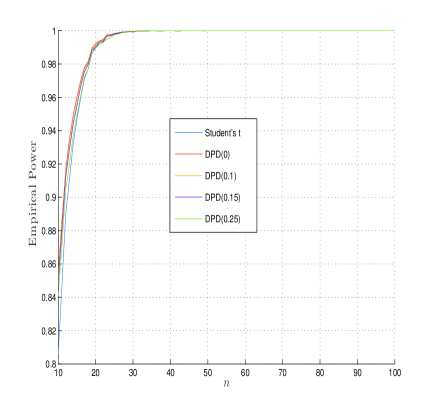
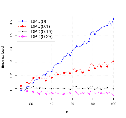
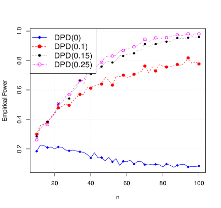
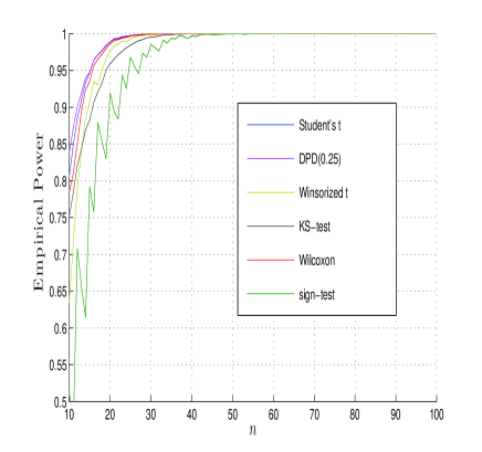
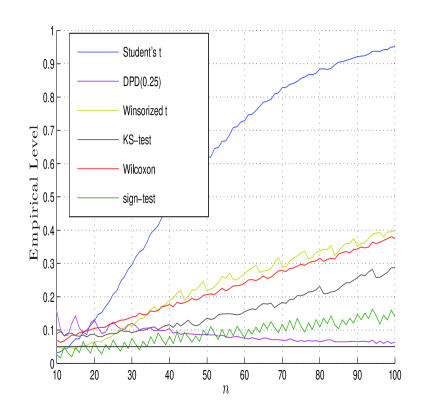
In this section we provide some extensive numerical evidence of the performance of the proposed methods, demonstrating, in particular, their strong robustness properties. Notice that the test statistic depends on the data only through the value of the estimator (both unconstrained and constrained), so that the robustness of the test would appear to depend directly on the robustness of the estimator. However, it is still useful to develop actual theoretical robustness properties of the proposed tests. Fortunately there is a wealth of material available in this context which makes our work easy. Toma and Broniatowski (2011) and Toma and Leoni-Aubin (2010) have, in general, touched upon the issue of theoretical robustness properties of tests. They have considered several theoretical measures of robustness in this context. In a more limited, but a more focused setting Ghosh et al. (2015) have considered the robustness measures of test statistics based on the family of S𝑆S-divergences which include the DPD as a special case; in particular the influence functions of the tests and the so called level and power influence functions are derived. Taken together, the above references further reinforce the notion that the robustness of these tests are directly dependent on the robustness of the estimators as the influence function of the tests turn out to be directly related to the influence function of the estimators. The Ghosh et al. (2015) paper relates only to the case of the simple null hypothesis; however it is not difficult to intuitively see how the robustness of these tests extend to the case of the composite hypothesis. The theoretical robustness properties of some similar tests have been considered in the Ph.D. dissertation of Ghosh (2015). On the whole, there is substantial overall indication and evidence of the theoretical robustness properties of the tests under study. For the sake of brevity we do not repeat these results here, but concentrate instead on the performance of the tests as observed in simulations and actual real data examples.

6.1 Real Data Examples

6.1.1 Telephone-Fault Data

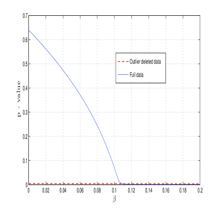
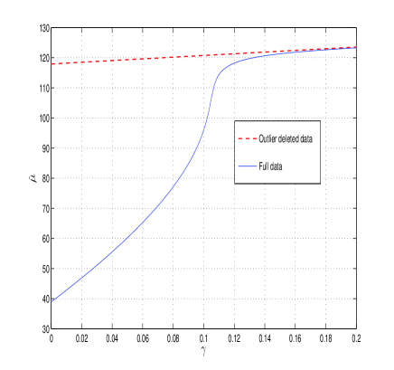
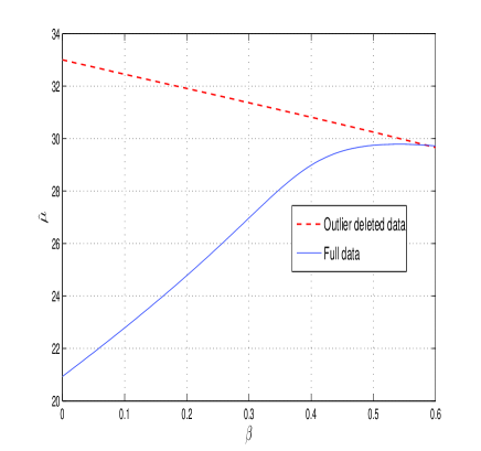
We consider the data on telephone line faults presented and analyzed by Welch (1987); the data were also analyzed by Simpson (1989). The data are given in Table 1, and consist of the ordered differences between the inverse test rates and the inverse control rates in 14 matched pairs of areas. A parametric approach to analyze this would be to model these data as a random sample from a normal distribution with mean μ𝜇\mu and standard deviation σ𝜎\sigma. It is obvious that the first observation of this dataset is a huge outlier with respect to the normal model, while the remaining 13 observations appear to be reasonable with respect to the same.

Basu et al. (2013) provided a limited analysis of these data by testing simple null hypotheses under the normal model. They tested null hypothesis about the mean by assuming the variance to be known, and also tested null hypothesis about the variance by assuming the mean to be known. These are contrived situations, and are less meaningful than the more realistic situation where both parameters are unknown. In this paper we consider tests for the normal mean without assuming the scale parameter to be known.

For the full data, the t𝑡t-test for the null hypothesis H0:μ=0:subscript𝐻0𝜇0H_{0}:\mu=0 against H1:μ0:subscript𝐻1𝜇0H_{1}:\mu\neq 0 fails to reject the null due to the presence of the large outlier (two sided p𝑝p-value is 0.6584); however the robust Hellinger deviance test (Simpson, 1989) comfortably rejects the null (two sided p𝑝p-value based on the chi-square null distribution is 0.0061), as does the t𝑡t-test based on the cleaned data after the removal of the large outlier (two sided p𝑝p-value is 0.0076).

Table 1: Telephone-Fault Data
Pair 1 2 3 4 5 6 7 8 9 10 11 12 13 14
Difference 988988-988 135135-135 7878-78 3 59 83 93 110 189 197 204 229 289 310
Refer to caption Refer to caption
Figure 1: (a) Two sided p𝑝p-values of the density power divergence tests and (b) estimates of μ𝜇\mu for different values of γ𝛾\gamma in case of the telephone-fault data.

Under the normal model, the maximum likelihood estimates of μ𝜇\mu (and σ𝜎\sigma) are highly distorted due to the presence of the large outlier, and as a result the likelihood ratio test under the normal model fails to reject the null hypothesis. From the robustness perspective, this is precisely what we will like to avoid, and here we demonstrate that proper choices of the tuning parameter within the class of tests developed in this paper achieve this goal. Here we analyze the performance of the density power divergence tests with β=γ𝛽𝛾\beta=\gamma. Figure 1(a) represents the p𝑝p-values of the test H0:μ=0:subscript𝐻0𝜇0H_{0}:\mu=0 versus H1:μ0:subscript𝐻1𝜇0H_{1}:\mu\neq 0 for different values of β𝛽\beta in a region of interest. While it is clearly seen that the tests fail to reject the null hypothesis for these data at very small values of β𝛽\beta, the decision turns around sharply, as β𝛽\beta crosses and goes beyond 0.1. On the other hand, the p𝑝p-values of the same test based on the outlier deleted data remain stable, supporting rejection, at all values of β𝛽\beta (Figure 1(a)). The stable behavior of the test statistic based on the density power divergence for the full data approximately coincides with the stability of the density power divergence estimate of μ𝜇\mu itself, obtained under a two-parameter normal model, which is presented in Figure 1(b). The minimum density power divergence estimators of μ𝜇\mu for the full data and the outlier deleted data are practically identical for β>0.12𝛽0.12\beta>0.12. At least in this example, the robustness of the test statistic is clearly linked to the robustness of the estimator.
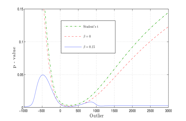
Refer to caption
Figure 2: Two sided p𝑝p-values for the tests for the mean for the telephone-fault data under the normal model against the first outlying observation.

To further explore the robustness properties of the density power divergence tests we look at the two sided p𝑝p-values for different values of the outlier. For this purpose we vary the first outlying observation in the range from 10001000-1000 to 3000 by keeping the remaining 13 observations fixed. Figure 2 shows the corresponding p𝑝p-values of the density power divergence tests with β=0.15𝛽0.15\beta=0.15 as well as β=0𝛽0\beta=0 and the ordinary t𝑡t-test. It shows that initially the p𝑝p-value of the density power divergence test with β=0.15𝛽0.15\beta=0.15 increases as the first observation moves away from the center of the data set, but after a certain limit the test gradually nullifies the effect of the outlier. On the other hand, the p𝑝p-values of the t𝑡t-test and the density power divergence test with β=0𝛽0\beta=0 keep on increasing with the outlier on either tail. Indeed the p𝑝p-values of these two tests are remarkably close to each other.

6.1.2 Darwin’s Plant Fertilization Data

Charles Darwin had performed an experiment which may be used to determine whether self-fertilized plants and cross-fertilized plants have different growth rates. In this experiment pairs of Zea mays plants, one self and the other cross-fertilized, were planted in pots, and after a specific time period the height of each plant was measured. A particular sample of 15 such pairs of plants led to the paired differences (cross-fertilized minus self fertilized) presented in increasing order in Table 2 (see Darwin, 1878).

Table 2: Darwin’s Plant Fertilization Data
Pair 1 2 3 4 5 6 7 8 9 10 11 12 13 14 15
Difference 6767-67 4848-48 6 8 14 16 23 24 28 29 41 49 56 60 75

As in the previous example, we assume a normal model for the paired differences and test H0:μ=0:subscript𝐻0𝜇0H_{0}:\mu=0 against H1:μ0:subscript𝐻1𝜇0H_{1}:\mu\neq 0, i.e. we test whether the mean of the paired differences is different from zero. The unconstrained minimum DPD estimates of μ𝜇\mu under the normal model corresponding to different values of the tuning parameter β𝛽\beta are presented in Figure 3(b). The two negative paired differences appear to be geometrically well separated from the rest of the data, though they are perhaps not as huge outliers as the first observation in the telephone-fault data. These two observations do have a substantial impact on the parameter estimates and the test statistic for testing H0subscript𝐻0H_{0} using density power divergence tests with very small values of γ=β𝛾𝛽\gamma=\beta, and it is instructive to compare to the case where these two outliers have been removed from the data. For small values of β𝛽\beta, the two sided p𝑝p-values of the test statistics are drastically different for the full data and outlier deleted cases (Figure 3(b)), but they get closer with increasing β𝛽\beta, and they essentially coincide for β0.45𝛽0.45\beta\geq 0.45. Once again this seems to be directly linked to the robustness of the parameter estimates; Figure 3(b), which also depicts the progression of the parameter estimates for the outlier deleted data, clearly demonstrates that. For comparison we note that the two sided p𝑝p-values for the ordinary t𝑡t-test in this case are 0.0497 (for full data) and 1.3119×1041.3119superscript1041.3119\times 10^{-4} (for the cleaned data with the two outliers removed).
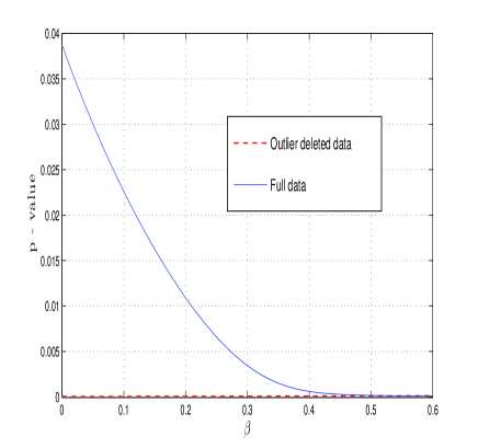
Refer to caption Refer to caption
Figure 3: (a) Two sided p𝑝p-values of the density power divergence tests and (b) estimates of μ𝜇\mu for different values of β𝛽\beta in case of Darwin’s fertilization data.

6.1.3 One Sided Tests

In general, the default alternative hypotheses considered in our proposed tests are of the two sided type. Depending on the nature of the problem and the dimension of the parameter, one sided alternatives may sometimes be of interest. For the telephone fault data the primary interest could be in determining whether the mean fault rate is higher than zero (rather than simply whether it is different from zero). It is presumable that Darwin’s interest in the fertilization problem was to determine whether cross fertilization leads to a higher growth rate compared to self fertilization; indeed the result of the test performed by R. A. Fisher (reported in Fisher, 1966) on the plant fertilization data relates to the one sided alternative. In this subsection we consider appropriate one sided tests for these two real data examples presented earlier in this section. For this purpose we consider the signed divergence statistic (the signed square root of the statistic presented in (25)) as was done in Simpson (1989). The relevant one sided p𝑝p-values are determined using the normal approximation, or that based on the t𝑡t-distribution. In the following we will describe the problem of testing H0:μ=0:subscript𝐻0𝜇0H_{0}:\mu=0 against H1:μ>0:subscript𝐻1𝜇0H_{1}:\mu>0 under the normal model with unknown scale.

The formal theory of constrained statistical inference (see Silvapulle and Sen, 2011) established the expression of the asymptotic likelihood ratio test for the hypotheses H0:μ=0:subscript𝐻0𝜇0H_{0}:\mu=0 against H1:μ>0:subscript𝐻1𝜇0H_{1}:\mu>0 to be

Tγ=0,β=0(1)=I(X¯>0)Tγ=0(𝜽^β=0,𝜽~β=0)=I(X¯>0)nlog(σ~n2σ^n2)superscriptsubscript𝑇formulae-sequence𝛾0𝛽01𝐼¯𝑋0subscript𝑇𝛾0subscriptbold-^𝜽𝛽0subscriptbold-~𝜽𝛽0𝐼¯𝑋0𝑛superscriptsubscript~𝜎𝑛2superscriptsubscript^𝜎𝑛2T_{\gamma=0,\beta=0}^{(1)}=I(\bar{X}>0)T_{\gamma=0}(\boldsymbol{\hat{\theta}}_{\beta=0},\boldsymbol{\tilde{\theta}}_{\beta=0})=I(\bar{X}>0)n\log\left(\tfrac{\tilde{\sigma}_{n}^{2}}{\hat{\sigma}_{n}^{2}}\right)

with asymptotic distribution equal to 12χ02+12χ1212superscriptsubscript𝜒0212superscriptsubscript𝜒12\tfrac{1}{2}\chi_{0}^{2}+\tfrac{1}{2}\chi_{1}^{2} under H0subscript𝐻0H_{0}, where χ02=0superscriptsubscript𝜒020\chi_{0}^{2}=0 a.s., I()𝐼I(\cdot) is the indicator function and 𝜽^β=0subscriptbold-^𝜽𝛽0\boldsymbol{\hat{\theta}}_{\beta=0}, 𝜽~β=0subscriptbold-~𝜽𝛽0\boldsymbol{\tilde{\theta}}_{\beta=0} are respectively the MDPDE and RMPDE for 𝜽=(μ,σ)T𝜽superscript𝜇𝜎𝑇\boldsymbol{\theta}=(\mu,\sigma)^{T} when the parameter spaces are the unrestricted and restricted ones of the two sided test (23). This test is almost the same as the one provided by the signed divergence likelihood ratio test statistic,

T~γ=0,β=0(1)=sign(X¯)Tγ=0(𝜽^β=0,𝜽~β=0)=sign(X¯)nlog(σ~n2σ^n2),superscriptsubscript~𝑇formulae-sequence𝛾0𝛽01𝑠𝑖𝑔𝑛¯𝑋subscript𝑇𝛾0subscriptbold-^𝜽𝛽0subscriptbold-~𝜽𝛽0𝑠𝑖𝑔𝑛¯𝑋𝑛superscriptsubscript~𝜎𝑛2superscriptsubscript^𝜎𝑛2\widetilde{T}_{\gamma=0,\beta=0}^{(1)}=sign(\bar{X})\sqrt{T_{\gamma=0}(\boldsymbol{\hat{\theta}}_{\beta=0},\boldsymbol{\tilde{\theta}}_{\beta=0})}=sign(\bar{X})\sqrt{n\log\left(\tfrac{\tilde{\sigma}_{n}^{2}}{\hat{\sigma}_{n}^{2}}\right)},

since the corresponding p𝑝p-values at t=nlog(σ~n2σ^n2)𝑡𝑛superscriptsubscript~𝜎𝑛2superscriptsubscript^𝜎𝑛2t=n\log\left(\frac{\tilde{\sigma}_{n}^{2}}{\hat{\sigma}_{n}^{2}}\right) are given by

p-valueTγ=0,β=0(1)(I(x¯>0)t)𝑝subscript-valuesuperscriptsubscript𝑇formulae-sequence𝛾0𝛽01𝐼¯𝑥0𝑡\displaystyle p\mbox{-value}_{T_{\gamma=0,\beta=0}^{(1)}}(I(\bar{x}>0)t) =12Pr(χ12>I(x¯>0)t),absent12Prsuperscriptsubscript𝜒12𝐼¯𝑥0𝑡\displaystyle=\frac{1}{2}\Pr(\chi_{1}^{2}>I(\bar{x}>0)t),
p-valueT~γ=0,β=0(1)(sign(x¯)t)𝑝subscript-valuesuperscriptsubscript~𝑇formulae-sequence𝛾0𝛽01𝑠𝑖𝑔𝑛¯𝑥𝑡\displaystyle p\mbox{-value}_{\widetilde{T}_{\gamma=0,\beta=0}^{(1)}}\left(sign(\bar{x})\sqrt{t}\right) =Pr(Z>sign(x¯)t),absentPr𝑍𝑠𝑖𝑔𝑛¯𝑥𝑡\displaystyle=\Pr(Z>sign(\bar{x})\sqrt{t}),

where Z𝑍Z follows standard normal distribution. This means that if x¯>0¯𝑥0\bar{x}>0, both p𝑝p-values are equal, whereas for x¯0¯𝑥0\bar{x}\leq 0,

p-valueTγ=0,β=0(1)(I(x¯>0)t)=1>p-valueT~γ=0,β=0(1)(sign(x¯)t)>12.𝑝subscript-valuesuperscriptsubscript𝑇formulae-sequence𝛾0𝛽01𝐼¯𝑥0𝑡1𝑝subscript-valuesuperscriptsubscript~𝑇formulae-sequence𝛾0𝛽01𝑠𝑖𝑔𝑛¯𝑥𝑡12p\mbox{-value}_{T_{\gamma=0,\beta=0}^{(1)}}(I(\bar{x}>0)t)=1>p\mbox{-value}_{\widetilde{T}_{\gamma=0,\beta=0}^{(1)}}\left(sign(\bar{x})\sqrt{t}\right)>\frac{1}{2}.

Both tests are in practice equivalent, and such a difference for big p𝑝p-values comes from the fact that T~γ=0,β=0(1)superscriptsubscript~𝑇formulae-sequence𝛾0𝛽01\widetilde{T}_{\gamma=0,\beta=0}^{(1)} is formally more appropriate for H0:μ0:subscript𝐻0𝜇0H_{0}:\mu\leq 0 against H1:μ>0:subscript𝐻1𝜇0H_{1}:\mu>0. We shall restrict ourselves, for simplicity, only to the signed divergence likelihood ratio test statistics and their DPD based analogues; the latter class of signed divergence DPDTS may be defined as

T~γ,β(1)=sign(μ^β){σ~βγγ+1(2β+1)3/2(2π)γ/2(β+1)3Tγ(𝜽^β,𝜽~β)}1/2superscriptsubscript~𝑇𝛾𝛽1𝑠𝑖𝑔𝑛subscript^𝜇𝛽superscriptsuperscriptsubscript~𝜎𝛽𝛾𝛾1superscript2𝛽132superscript2𝜋𝛾2superscript𝛽13subscript𝑇𝛾subscriptbold-^𝜽𝛽subscriptbold-~𝜽𝛽12\widetilde{T}_{\gamma,\beta}^{(1)}=sign(\hat{\mu}_{\beta})\left\{\frac{\widetilde{\sigma}_{\beta}^{\gamma}\sqrt{\gamma+1}\left(2\beta+1\right)^{3/2}\left(2\pi\right)^{\gamma/2}}{\left(\beta+1\right)^{3}}T_{\gamma}(\boldsymbol{\hat{\theta}}_{\beta},\boldsymbol{\tilde{\theta}}_{\beta})\right\}^{-1/2}

with asymptotic distribution equal to the standard normal under H0subscript𝐻0H_{0}. In calculating the one sided p𝑝p-values based on the signed divergence Hellinger distance test in case of the telephone fault data, Simpson (1989) used an approximation based on the t𝑡t-distribution, as the sample size was only 14. In large samples, the distribution of the statistic is approximately normal. The problem for a normal distribution with dimension bigger than one with inequality restrictions is more complicated and requires a specific theory based on Silvapulle and Sen (2011). Martín and Balakrishnan (2013) illustrate the procedure of handing this problem when ϕitalic-ϕ\phi-divergence based test statistics and MLEs are applied.


Telephone-fault data The one sided p𝑝p-values for the signed divergence DPDTSs corresponding to β=0.15𝛽0.15\beta=0.15 and 0.3 are presented in Table 3 for the full as well as outlier deleted data, using both the standard normal (Z𝑍Z) and t𝑡t (with suitable degrees of freedom) approximations. The result for the ordinary one-sided t𝑡t-test are also presented for comparison. The presence of the large outlier masks the significance in case of the t𝑡t-test, but the signed divergence DPDTSs provide consistent significant results with and without the outlier. Similar results were reported by Simpson (1989) with the signed divergence Hellinger distance test. The mean of the ordered differences between the inverse test rates and inverse control rates does appear to be greater than zero.

Table 3: p𝑝p-values of the one sided tests for the mean in case of the telephone-fault data.
Scenario
cutoff t𝑡t-test DPD(0.15) DPD(0.3)
Full Deleted Full Deleted Full Deleted
Z𝑍Z 0.0006 0.0019 0.0013 0.0017
t𝑡t 0.3481 0.0037 0.0032 0.0068 0.0050 0.0064

Darwin’s plant fertilization data The results are presented in Table LABEL:tab:dar. The full data p𝑝p-value was reported by Fisher (1966). In this case the one sided p𝑝p-values for the t𝑡t-test lead to a shift from marginal significance to solid rejection due to the deletion of the (two) outliers. This also seems to be the case for signed divergence DPDTSs for very small values of β𝛽\beta. However, larger values of β𝛽\beta lead to a more consistent behavior of the tests. This dataset requires stronger downweighting compared to the telephone-fault data, as the outliers here are less extreme, and therefore more difficult to identify. Under a suitable robust test, it appears that the mean growth of cross fertilized plants would be declared to be significantly higher than self fertilized plants.

Table 4: p𝑝p-values of the one sided tests for the mean in case of the Darwin’s plant fertilization data.
Scenario
cutoff t𝑡t-test DPD(0.15) DPD(0.3)
Full Deleted Full Deleted Full Deleted
Z𝑍Z 0.0081 <104absentsuperscript104<10^{-4} 0.0017 <104absentsuperscript104<10^{-4}
t𝑡t 0.0252 <104absentsuperscript104<10^{-4} 0.0153 0.0008 0.0055 0.0009

6.2 Simulation Results

6.2.1 Normal Case

To further explore the performance of our proposed test statistic in case of the 𝒩(μ,σ2)𝒩𝜇superscript𝜎2\mathcal{N}(\mu,\sigma^{2}) problem, we studied the behavior of the tests through simulation. We considered the hypothesis H0:μ=0:subscript𝐻0𝜇0H_{0}:\mu=0 against the alternative H1:μ0:subscript𝐻1𝜇0H_{1}:\mu\neq 0 with σ2superscript𝜎2\sigma^{2} unknown when data were generated from the 𝒩(0,1)𝒩01\mathcal{N}(0,1) distribution. Subsequently, the same hypotheses were tested when the data were generated from the 𝒩(1,1)𝒩11\mathcal{N}(1,1) distribution. In the first case our interest was in studying the observed level (measured as the proportion of test statistics exceeding the chi-square critical value in a large number – here 10000 – of replications) of the test under the correct null hypothesis, and in the second case we were interested in the observed power (obtained in a similar manner as above) of the test under the incorrect null hypothesis. The results are given in Figures 4(a) and 4(b). In either case the nominal level was 0.050.050.05. We have used the ordinary t𝑡t-test together with several DPD test statistics, corresponding to β=0,0.1,0.15𝛽00.10.15\beta=0,0.1,0.15 and 0.250.250.25, in this particular study. The horizontal lines in Figure 4(a), and later in Figure 4(c), represent the nominal level of 0.05.

It may be noticed that all the tests excepting the exact likelihood ratio test (the t𝑡t-test) are slightly liberal for very small sample sizes and lead to somewhat inflated observed levels. However this discrepancy decreases rapidly, and by the time the sample size is 30 or more the observed levels have settled down reasonably around acceptable values. The observed powers of the tests as given in Figure 4(b) are, in fact, extremely close; in very small sample sizes the other tests have slightly higher power than the t𝑡t-test, but this must be a consequence of the observed levels of these tests being higher than the latter for such sample sizes. On the whole the proposed tests appear to be quite competitive to the ordinary t𝑡t-test for pure normal data.

To evaluate the stability of the level of the tests under contamination, we repeated the tests for H0:μ=0:subscript𝐻0𝜇0H_{0}:\mu=0 against H1:μ0:subscript𝐻1𝜇0H_{1}:\mu\neq 0 under data generated from the mixture of N(0,1)𝑁01N(0,1) and N(10,1)𝑁101N(-10,1), where the mixing weight of the first component is 0.9. To illustrate the stability of power, the tests were performed with data generated under a mixture of N(1,1)𝑁11N(1,1) and N(10,1)𝑁101N(-10,1), where the mixing weight of the first component is again 0.9. The results are given in 4(c) and 4(d) respectively.

In this case there is a drastic and severe inflation in the observed level of the t𝑡t-test and that of the DPD(0) test. As β𝛽\beta increases, however, the resistant nature of the tests are clearly apparent. By the time β=0.25𝛽0.25\beta=0.25, the levels have already been reduced to acceptable values. The opposite behavior is seen in case of power. There appears to be a complete breakdown in power for small values of β𝛽\beta, but the power remains quite stable for values of β𝛽\beta equal to 0.25 or greater.

On the whole it appears to be fair to claim that for sample sizes equal to or larger than 30 the efficiency of many of our DPDTSs are very close to the efficiency of the t𝑡t-test, but the robustness properties of our tests are often significantly better than the t𝑡t-test in terms of maintaining the stability of both the level and power.
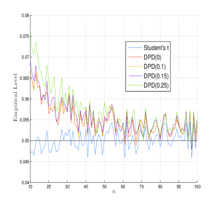
Refer to caption Refer to caption
(a) (b)
Refer to caption Refer to caption
(c) (d)
Figure 4: Simulated levels and powers of the DPDTSs for pure and contaminated data in case of the normal distribution.
Refer to caption Refer to caption
(a) (b)
Refer to caption Refer to caption
(c) (d)
Figure 5: Simulated levels and powers of the DPDTSs for pure and contaminated data in case of the Weibull distribution.

6.2.2 Weibull Case

As we have mentioned before, it is important to demonstrate the properties of the proposed method in models other than the normal so that one has a better idea about the scope of the method. Accordingly we performed tests of composite hypotheses under the Weibull model in the spirit of Section 6.2.1. Let us consider the hypothesis defined in (28), where σ0subscript𝜎0\sigma_{0} is taken to be 1.5. In the first study we have generated data from the 𝒲(1.5,1.5)𝒲1.51.5\mathcal{W}(1.5,1.5) distribution. The plot for the observed level for the hypothesis H0:σ=1.5:subscript𝐻0𝜎1.5H_{0}:\sigma=1.5 against the two sided alternative is given in Figure 5(a), where we have used 1,000 replications. Next the same hypotheses were tested when the data were generated from the 𝒲(1.1,1.5)𝒲1.11.5\mathcal{W}(1.1,1.5) distribution. The observed power function is plotted in Figure 5(b) for different values of β𝛽\beta. The powers are remarkably close. In all cases the nominal level was 0.050.050.05.

To evaluate the stability of the level and the power of the tests under contamination, we repeated the tests with data generated from the Weibull mixture consisting of 95% 𝒲(1.5,1.5)𝒲1.51.5\mathcal{W}(1.5,1.5) and 5% 𝒲(25,1.5)𝒲251.5\mathcal{W}(25,1.5), and then from mixture of 95% 𝒲(1.1,1.5)𝒲1.11.5\mathcal{W}(1.1,1.5) and 5% 𝒲(25,1.5)𝒲251.5\mathcal{W}(25,1.5). In either case the first larger component is our target. In Figures 5(c), the levels of the statistics under the contamination of first type are presented indicating the stability of levels for moderately large values of β𝛽\beta. Figure 5(d) demonstrates the stability of powers under contaminated data of the second type for the same values of β𝛽\beta.

6.2.3 Comparison with Other Robust Tests

Here we provide a comparison of our proposed tests with some other popular resistant tests available in the literature. In particular we have used a parametric test – the Winsorized test of Dixon and Tukey (1968) together with three nonparametric tests – the one sample Kolmogorov-Smirnov (KS) test, the two sided Wilcoxon signed rank test and the two sided sign test. The model, the hypotheses, the parameters chosen, the level of significance and other details of the set up of this simulation are the same as those in Section 6.2.1.

We have Winsorized the 15% extreme observations on each tail of the data distribution in case of the Winsorized t𝑡t-test. Note that the null hypotheses are slightly different for the nonparametric tests. For the KS-test we first standardize the data using robust statistics, and then test whether the corresponding distribution is a standard normal. The data are standardized using the transformation Z=(Xμ0)/MAD.𝑍𝑋subscript𝜇0MADZ=(X-\mu_{0})/\mbox{MAD}. Here μ0subscript𝜇0\mu_{0} is the null value and MADMAD{\rm MAD} is 1.4826×1.4826\times(median absolute deviation about the median). In case of the Wilcoxon test and the sign test we perform tests for the population median without making any parametric model assumptions. For comparison just one DPDTS is used in these simulations, that corresponding to the tuning parameter β=0.25𝛽0.25\beta=0.25. To emphasize the robustness properties of these tests we have also included the Student’s t𝑡t-test in these investigations, so that the robust tests stand out in contrast. Our simulation results are presented in Figure 6.

From Figure 6(a) it may be observed that the empirical levels of the Winsorized t𝑡t-test, the KS-test and the Wilcoxon test are very close to the nominal level for pure normal data. For small sample sizes the DPDTS is slightly liberal; however even at a sample size of 30, it is off by only one percent compared to the nominal level. On the other hand the sign test is a bit conservative, even at fairly large samples. The observed powers of all the tests in Figure 6(b) rapidly approach unity in fairly small samples. The results in Figure 6(c) demonstrate that for contaminated data all tests except the DPDTS fail to maintain the nominal level. The observed level of the sign test is close to the nominal level for small sample sizes but eventually as the sample size increases it also breaks down. The powers of the tests for the contaminated data, plotted in Figure 6(d) show that all the robust tests exhibit stable power. For small sample sizes the DPDTS exhibits the highest power. The overall observation on the basis of all the above appears to be that the DPD based test is superior to the classical Wald test under contamination, and is also competitive or better than several other standard resistant tests in terms of robustness, at least to the extent this particular simulation study is concerned.
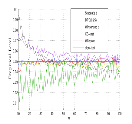
Refer to caption Refer to caption
(a) (b)
Refer to caption Refer to caption
(c) (d)
Figure 6: Simulated levels and powers of some robust tests for pure and contaminated data in case of the normal distribution.

7 Choosing the Tuning Parameter

By construction, the test statistic in (14) employs two different tuning parameters β𝛽\beta and γ𝛾\gamma. These parameters have two different roles, in two different stages in the hypothesis testing process. The parameter β𝛽\beta is used to evaluate the robust unconstrained and constrained (under the null hypothesis) estimators. In the next stage a density power divergence with parameter γ𝛾\gamma is constructed to quantify the disparity between the fitted unrestricted and the restricted models. As seen in Theorem 3, the null distribution of the statistic can be derived for all values of the parameters β,γ>0𝛽𝛾0\beta,\gamma>0, and in practice one can choose them independently of one another. As the robustness of the test statistic depends primarily on the robustness of the estimators, the choice of the parameter β𝛽\beta turns out to be more critical in our testing procedure. In repeated simulations (not presented here) our observation is that the parameter γ𝛾\gamma does not have a significant impact on the robustness of the procedure. Thus while the generality of the method allows us the choice of possibly different tuning parameters, for simplicity of implementation we will let β=γ𝛽𝛾\beta=\gamma, so that the selection problem reduces to that of a single parameter. Throughout the paper, we have used β=γ𝛽𝛾\beta=\gamma in our simulations and real data examples.

In a real situation, the experimenter will require some guidance on the choice of this single tuning parameter β𝛽\beta. Broniatowski et al. (2012) have reported that values of β[0.1,0.25]𝛽0.10.25\beta\in[0.1,0.25] are often reasonable choices; we largely agree with this view, although tentative outliers and heavier contamination may require greater downweighting through a larger value of β𝛽\beta; this is the case, for example, in Darwin’s plant fertilization data example. However, apart from fixed choices, other data driven and adaptive choices could also be useful, as one can then tune the parameter to make the procedure more robust as required. In this paper we follow the approach of Warwick and Jones (2005) for this purpose, which minimizes an empirical measure of the mean square error of the estimator to determine the “optimal” tuning parameter. This requires the use of a robust pilot estimator of the parameter. Warwick and Jones (2005) suggested the use of the MPDPDE corresponding to β=1𝛽1\beta=1. The optimal parameter depends on the choice of the pilot estimator, however, and as larger values of β𝛽\beta lead to a loss in efficiency, Ghosh and Basu (2013) suggested the choice of the MDPDE with β=0.5𝛽0.5\beta=0.5 as the pilot estimator, which appears to be reasonable in most cases. Our subsequent analysis is based on the Warwick and Jones (2005) method, with the Ghosh and Basu (2013) modification.

We do acknowledge that the criterion to be considered for the choice of the optimal β𝛽\beta for the testing problem is not necessarily the same for the estimation problem. In hypothesis testing the appropriate criterion should involve a suitable linear combination of the inflation in the observed level under the null and the drop in power under contiguous alternatives in a contaminated scenario. However, an appropriate measure of this sort is not easy to construct. As it appears that the robustness of the proposed tests correspond almost exactly to the robustness of the MDPDEs, we feel that the optimal choice of β𝛽\beta as described in the previous paragraph would generally work reasonably well in case of the hypothesis testing problem also. As of now, we recommend the choice of β𝛽\beta according to the above recipe.

The above criterion leads to estimated optimal choices of β𝛽\beta to be 0.1919 for the telephone fault data, and 0.5657 for Darwin’s plant fertilization data respectively. As the first observation in the telephone fault data is a massive outlier, it is easily recognized by the testing procedures even at fairly small values of β𝛽\beta. However for Darwins’ plant fertilization data the outliers are more tentative, and therefore require stronger downweighting to eliminate their effect.

8 Concluding Remarks

This paper provides the appropriate theoretical machinery to perform general parametric tests of hypotheses based on the density power divergence. We demonstrate that one can construct a class of parametric tests of hypotheses based on the above measure which allows the experimenter to test for composite null hypotheses under the presence of nuisance parameters. The tests of this class have been shown to have excellent robustness properties in simulation studies and have a huge scope of application; for the purpose of numerical demonstration we have chosen the scenario of the usual t𝑡t-test and illustrated that for this situation the proposed test provides extremely satisfactory results. Similar improvements are also demonstrated outside the normal model, when data are generated from the Weibull distribution. When considered with the benefit of not requiring any intermediate smoothing technique as in the case of the Hellinger deviance test, our proposed techniques appear to prominently stand out among classes of robust tests for composite hypotheses. Our results also appropriately generalize the results of Basu et al. (2013).


Acknowledgments This work was partially supported by Grant MTM-2012-33740.

References

  • Basu et al. (1998) A. Basu, I. R. Harris, N. L. Hjort, and M. C. Jones. Robust and efficient estimation by minimising a density power divergence. Biometrika, 85(3):549–559, 1998.
  • Basu et al. (2011) A. Basu, H. Shioya, and C. Park. Statistical inference: The minimum distance approach. CRC Press, Boca Raton, FL, 2011.
  • Basu et al. (2013) A. Basu, A. Mandal, N. Martin, and L. Pardo. Testing statistical hypotheses based on the density power divergence. Ann. Inst. Statist. Math., 65(2):319–348, 2013.
  • Broniatowski et al. (2012) M. Broniatowski, A. Toma, and I. Vajda. Decomposable pseudodistances and applications in statistical estimation. J. Statist. Plann. Inference, 142(9):2574–2585, 2012.
  • Darwin (1878) C. Darwin. The Effects of Cross and Self Fertilization in the Vegetable Kingdom. John Murray, London, 1878.
  • Davies (1980) R. B. Davies. The distribution of a linear combination of χ2superscript𝜒2\chi^{2} random variables. Algorithm AS155. Appl. Statist., 29:323–333, 1980.
  • De Angelis and Young (1992) D. De Angelis and G. A. Young. Smoothing the bootstrap. Internat. Statist. Rev., 60(1):45–56, 1992.
  • Dik and de Gunst (1985) J. J. Dik and M. C. M. de Gunst. The distribution of general quadratic forms in normal variables. Statist. Neerlandica, 39(1):14–26, 1985.
  • Dixon and Tukey (1968) W. J. Dixon and J. W. Tukey. Approximate behavior of the distribution of winsorized t (trimming/winsorization 2). Technometrics, 10(1):83–98, 1968.
  • Eckler (1969) A. R. Eckler. A survey of coverage problems associated with point and area targets. Technometrics, 11(3):561–589, 1969.
  • Fisher (1966) R. Fisher. The Design of Experiments. Hafner Press, New York, 1966.
  • Fraser (1957) D. A. S. Fraser. Most powerful rank-type tests. Ann. Math. Statist, 28:1040–1043, 1957.
  • Ghosh (2015) A. Ghosh. Robust Minimum Divergence Inference using Density Power Divergence and Its Extensions. PhD thesis, submitted to the Indian Statistical Institute, 2015.
  • Ghosh and Basu (2013) A. Ghosh and A. Basu. Robust estimation for independent non-homogeneous observations using density power divergence with applications to linear regression. Electron. J. Stat., 7:2420–2456, 2013.
  • Ghosh et al. (2015) A. Ghosh, A. Basu, and L. Pardo. On the robustness of a divergence based test of simple statistical hypotheses. J. Statist. Plann. Inference, 2015.
  • Gupta (1963) S. S. Gupta. Bibliography on the multivariate normal integrals and related topics. Ann. Math. Statist., 34:829–838, 1963.
  • Johnson and Kotz (1968) N. L. Johnson and S. Kotz. Tables of distributions of positive definite quadratic forms in central normal variables. Sankhyā, Series B, 30:303–314, 1968.
  • Jones et al. (2001) M. C. Jones, N. L. Hjort, I. R. Harris, and A. Basu. A comparison of related density-based minimum divergence estimators. Biometrika, 88(3):865–873, 2001.
  • Lehmann (1983) E. L. Lehmann. Theory of point estimation. Wiley Series in Probability and Mathematical Statistics. John Wiley & Sons Inc., New York, 1983.
  • Lindsay (1994) B. G. Lindsay. Efficiency versus robustness: the case for minimum Hellinger distance and related methods. Ann. Statist., 22(2):1081–1114, 1994.
  • Martín and Balakrishnan (2013) N. Martín and N. Balakrishnan. Hypothesis testing in a generic nesting framework for general distributions. J. Multivariate Anal., 118:1–23, 2013.
  • Pardo (2006) L. Pardo. Statistical inference based on divergence measures. Chapman & Hall/CRC, Boca Raton, FL, 2006.
  • Sen et al. (2010) P. K. Sen, J. M. Singer, and A. C. P. de Lima. From finite sample to asymptotic methods in statistics. Cambridge University Press, 2010.
  • Silvapulle and Sen (2011) M. J. Silvapulle and P. K. Sen. Constrained statistical inference: Order, inequality, and shape constraints, volume 912. John Wiley & Sons, 2011.
  • Silvey (1975) S. D. Silvey. Statistical inference. Chapman and Hall, London, 1975. Reprinting, Monographs on Statistical Subjects.
  • Simpson (1989) D. G. Simpson. Hellinger deviance tests: efficiency, breakdown points, and examples. J. Amer. Statist. Assoc., 84(405):107–113, 1989.
  • Solomon (1960) H. Solomon. Distribution of quadratic forms: tables and applications. Applied Mathematics and Statistics Laboratories, Stanford University Stanford, California, 1960.
  • Toma and Broniatowski (2011) A. Toma and M. Broniatowski. Dual divergence estimators and tests: robustness results. J. Multivariate Anal., 102(1):20–36, 2011.
  • Toma and Leoni-Aubin (2010) A. Toma and S. Leoni-Aubin. Robust tests based on dual divergence estimators and saddlepoint approximations. J. Multivariate Anal., 101(5):1143–1155, 2010.
  • Warwick and Jones (2005) J. Warwick and M. Jones. Choosing a robustness tuning parameter. J. Stat. Comput. Simulation, 75(7):581–588, 2005.
  • Welch (1987) W. J. Welch. Rerandomizing the median in matched-pairs designs. Biometrika, 74(3):609–614, 1987.
  • White (1982) H. White. Maximum likelihood estimation of misspecified models. Econometrica, 50(1):1–25, 1982.

Appendix

There is some overlap between the Lehmann and Basu et al. conditions. In the following we present the consolidated set of conditions which are the useful ones in our context.


Lehmann and Basu et al. conditions

  • (LB1)

    The model distributions F𝜽subscript𝐹𝜽F_{\boldsymbol{\theta}} of X𝑋X have common support, so that the set 𝒳={x|f𝜽(x)>0}𝒳conditional-set𝑥subscript𝑓𝜽𝑥0\mathcal{X}=\{x|f_{\boldsymbol{\theta}}(x)>0\} is independent of 𝜽𝜽\boldsymbol{\theta}. The true distribution H𝐻H is also supported on 𝒳𝒳\mathcal{X}, on which the corresponding density hh is greater than zero.

  • (LB2)

    There is an open subset of ω𝜔\omega of the parameter space ΘΘ\Theta, containing the best fitting parameter 𝜽0subscript𝜽0\boldsymbol{\theta}_{0} such that for almost all x𝒳𝑥𝒳x\in\mathcal{X}, and all 𝜽ω𝜽𝜔\boldsymbol{\theta}\in\omega, the density f𝜽(x)subscript𝑓𝜽𝑥f_{\boldsymbol{\theta}}(x) is three times differentiable with respect to 𝜽𝜽\boldsymbol{\theta} and the third partial derivatives are continuous with respect to 𝜽𝜽\boldsymbol{\theta}.

  • (LB3)

    The integrals f𝜽1+β(x)𝑑xsuperscriptsubscript𝑓𝜽1𝛽𝑥differential-d𝑥\int f_{\boldsymbol{\theta}}^{1+\beta}(x)dx and f𝜽β(x)h(x)𝑑xsuperscriptsubscript𝑓𝜽𝛽𝑥𝑥differential-d𝑥\int f_{\boldsymbol{\theta}}^{\beta}(x)h(x)dx can be differentiated three times with respect to 𝜽𝜽\boldsymbol{\theta}, and the derivatives can be taken under the integral sign.

  • (LB4)

    The p×p𝑝𝑝p\times p matrix 𝑱β(𝜽)subscript𝑱𝛽𝜽\boldsymbol{J}_{\beta}(\boldsymbol{\theta}), defined in (8), is positive definite.

  • (LB5)

    There exists a function Mjkl(x)subscript𝑀𝑗𝑘𝑙𝑥M_{jkl}(x) such that |jklV𝜽(x)|Mjkl(x)subscript𝑗𝑘𝑙subscript𝑉𝜽𝑥subscript𝑀𝑗𝑘𝑙𝑥|\nabla_{jkl}V_{\boldsymbol{\theta}}(x)|\leq M_{jkl}(x) for all 𝜽ω𝜽𝜔\boldsymbol{\theta}\in\omega, where Eh[Mjkl(X)]=mjkl<subscript𝐸delimited-[]subscript𝑀𝑗𝑘𝑙𝑋subscript𝑚𝑗𝑘𝑙E_{h}[M_{jkl}(X)]=m_{jkl}<\infty for all j𝑗j, k𝑘k and l𝑙l, where Vθ(x)subscript𝑉𝜃𝑥V_{\theta}(x) is as defined in (6).

Proof of Theorem 2 This proof closely follows the approach of Sen et al. (2010). Let

hn(𝜽)=11+β[f𝜽1+β(x)𝑑x(1+1β)1ni=1nf𝜽β(Xi)]subscript𝑛𝜽11𝛽delimited-[]superscriptsubscript𝑓𝜽1𝛽𝑥differential-d𝑥11𝛽1𝑛superscriptsubscript𝑖1𝑛superscriptsubscript𝑓𝜽𝛽subscript𝑋𝑖h_{n}(\boldsymbol{\theta})=\frac{1}{1+\beta}\left[\int f_{\boldsymbol{\theta}}^{1+\beta}(x)dx-\left(1+\frac{1}{\beta}\right)\frac{1}{n}\sum_{i=1}^{n}f_{\boldsymbol{\theta}}^{\beta}(X_{i})\right] (36)

be the function (6) divided by 1+β1𝛽1+\beta. By differentiating both sides of equation (36) with respect to 𝜽𝜽\boldsymbol{\theta} we get

𝜽hn(𝜽)=𝒖𝜽(x)f𝜽1+β(x)𝑑x1ni=1n𝒖𝜽(Xi)f𝜽β(Xi)𝜽subscript𝑛𝜽subscript𝒖𝜽𝑥superscriptsubscript𝑓𝜽1𝛽𝑥differential-d𝑥1𝑛superscriptsubscript𝑖1𝑛subscript𝒖𝜽subscript𝑋𝑖superscriptsubscript𝑓𝜽𝛽subscript𝑋𝑖\frac{\partial}{\partial\boldsymbol{\theta}}h_{n}(\boldsymbol{\theta})=\int\boldsymbol{u}_{\boldsymbol{\theta}}(x)f_{\boldsymbol{\theta}}^{1+\beta}(x)dx-\frac{1}{n}\sum_{i=1}^{n}\boldsymbol{u}_{\boldsymbol{\theta}}(X_{i})f_{\boldsymbol{\theta}}^{\beta}(X_{i})

and differentiating again with respect to 𝜽𝜽\boldsymbol{\theta}

𝜽T𝜽hn(𝜽)superscript𝜽𝑇𝜽subscript𝑛𝜽\displaystyle\frac{\partial}{\partial\boldsymbol{\theta}^{T}}\frac{\partial}{\partial\boldsymbol{\theta}}h_{n}(\boldsymbol{\theta}) =(1+β)𝒖𝜽(x)𝒖𝜽T(x)f𝜽1+β(x)𝑑x𝑰𝜽(x)f𝜽1+β(x)𝑑xabsent1𝛽subscript𝒖𝜽𝑥superscriptsubscript𝒖𝜽𝑇𝑥superscriptsubscript𝑓𝜽1𝛽𝑥differential-d𝑥subscript𝑰𝜽𝑥superscriptsubscript𝑓𝜽1𝛽𝑥differential-d𝑥\displaystyle=(1+\beta)\int\boldsymbol{u}_{\boldsymbol{\theta}}(x)\boldsymbol{u}_{\boldsymbol{\theta}}^{T}(x)f_{\boldsymbol{\theta}}^{1+\beta}(x)dx-\int\boldsymbol{I}_{\boldsymbol{\theta}}(x)f_{\boldsymbol{\theta}}^{1+\beta}(x)dx
βni=1n𝒖𝜽(Xi)𝒖𝜽T(Xi)f𝜽β(Xi)+1ni=1n𝑰𝜽(Xi)f𝜽β(Xi).𝛽𝑛superscriptsubscript𝑖1𝑛subscript𝒖𝜽subscript𝑋𝑖superscriptsubscript𝒖𝜽𝑇subscript𝑋𝑖superscriptsubscript𝑓𝜽𝛽subscript𝑋𝑖1𝑛superscriptsubscript𝑖1𝑛subscript𝑰𝜽subscript𝑋𝑖superscriptsubscript𝑓𝜽𝛽subscript𝑋𝑖\displaystyle-\frac{\beta}{n}\sum_{i=1}^{n}\boldsymbol{u}_{\boldsymbol{\theta}}(X_{i})\boldsymbol{u}_{\boldsymbol{\theta}}^{T}(X_{i})f_{\boldsymbol{\theta}}^{\beta}(X_{i})+\frac{1}{n}\sum_{i=1}^{n}\boldsymbol{I}_{\boldsymbol{\theta}}(X_{i})f_{\boldsymbol{\theta}}^{\beta}(X_{i}).

Here 𝒖𝜽(x)=𝜽logf𝜽(x)subscript𝒖𝜽𝑥𝜽subscript𝑓𝜽𝑥\boldsymbol{u}_{{\boldsymbol{\theta}}}(x)=\frac{\partial}{\partial\boldsymbol{\theta}}\log f_{{\boldsymbol{\theta}}}(x) and 𝑰𝜽(x)=𝜽𝒖𝜽(x)subscript𝑰𝜽𝑥𝜽subscript𝒖𝜽𝑥\boldsymbol{I}_{\boldsymbol{\theta}}(x)=-\frac{\partial}{\partial\boldsymbol{\theta}}\boldsymbol{u}_{\boldsymbol{\theta}}(x). We assume that the null hypothesis is true, and 𝜽0Θ0subscript𝜽0subscriptΘ0\boldsymbol{\theta}_{0}\in\Theta_{0} is the true value of the parameter. Since the model is correct 𝜽T𝜽hn(𝜽)|𝜽=𝜽0evaluated-atsuperscript𝜽𝑇𝜽subscript𝑛𝜽𝜽subscript𝜽0\frac{\partial}{\partial\boldsymbol{\theta}^{T}}\frac{\partial}{\partial\boldsymbol{\theta}}\left.h_{n}(\boldsymbol{\theta})\right|_{\boldsymbol{\theta=\theta}_{0}} converges in probability to

limn𝜽T𝜽hn(𝜽)|𝜽=𝜽0evaluated-atsubscript𝑛superscript𝜽𝑇𝜽subscript𝑛𝜽𝜽subscript𝜽0\displaystyle\lim_{n\rightarrow\infty}\frac{\partial}{\partial\boldsymbol{\theta}^{T}}\frac{\partial}{\partial\boldsymbol{\theta}}h_{n}(\boldsymbol{\theta})\Big{|}_{\boldsymbol{\theta=\theta}_{0}} =(1+β)𝒖𝜽0(x)𝒖𝜽0T(x)f𝜽01+β(x)𝑑x𝑰𝜽0(x)f𝜽01+β(x)𝑑xabsent1𝛽subscript𝒖subscript𝜽0𝑥superscriptsubscript𝒖subscript𝜽0𝑇𝑥superscriptsubscript𝑓subscript𝜽01𝛽𝑥differential-d𝑥subscript𝑰subscript𝜽0𝑥superscriptsubscript𝑓subscript𝜽01𝛽𝑥differential-d𝑥\displaystyle=(1+\beta)\int\boldsymbol{u}_{\boldsymbol{\theta}_{0}}(x)\boldsymbol{u}_{\boldsymbol{\theta}_{0}}^{T}(x)f_{\boldsymbol{\theta}_{0}}^{1+\beta}(x)dx-\int\boldsymbol{I}_{\boldsymbol{\theta}_{0}}(x)f_{\boldsymbol{\theta}_{0}}^{1+\beta}(x)dx
β𝒖𝜽0(x)𝒖𝜽0T(x)f𝜽01+β(x)𝑑x+𝑰𝜽0(x)f𝜽01+β(x)𝑑x𝛽subscript𝒖subscript𝜽0𝑥superscriptsubscript𝒖subscript𝜽0𝑇𝑥superscriptsubscript𝑓subscript𝜽01𝛽𝑥differential-d𝑥subscript𝑰subscript𝜽0𝑥superscriptsubscript𝑓subscript𝜽01𝛽𝑥differential-d𝑥\displaystyle-\beta\int\boldsymbol{u}_{\boldsymbol{\theta}_{0}}(x)\boldsymbol{u}_{\boldsymbol{\theta}_{0}}^{T}(x)f_{\boldsymbol{\theta}_{0}}^{1+\beta}(x)dx+\int\boldsymbol{I}_{\boldsymbol{\theta}_{0}}(x)f_{\boldsymbol{\theta}_{0}}^{1+\beta}(x)dx
=𝒖𝜽0(x)𝒖𝜽0T(x)f𝜽01+β(x)𝑑x.absentsubscript𝒖subscript𝜽0𝑥superscriptsubscript𝒖subscript𝜽0𝑇𝑥superscriptsubscript𝑓subscript𝜽01𝛽𝑥differential-d𝑥\displaystyle=\int\boldsymbol{u}_{\boldsymbol{\theta}_{0}}(x)\boldsymbol{u}_{\boldsymbol{\theta}_{0}}^{T}(x)f_{\boldsymbol{\theta}_{0}}^{1+\beta}(x)dx.

Notice that limn𝜽T𝜽hn(𝜽)|𝜽=𝜽0=𝑱β(𝜽0)evaluated-atsubscript𝑛superscript𝜽𝑇𝜽subscript𝑛𝜽𝜽subscript𝜽0subscript𝑱𝛽subscript𝜽0\lim_{n\rightarrow\infty}\frac{\partial}{\partial\boldsymbol{\theta}^{T}}\frac{\partial}{\partial\boldsymbol{\theta}}h_{n}(\boldsymbol{\theta})|_{\boldsymbol{\theta=\theta}_{0}}=\boldsymbol{J}_{\beta}(\boldsymbol{\theta}_{0}) defined earlier in equation (10). Since f𝜽0subscript𝑓subscript𝜽0f_{\boldsymbol{\theta}_{0}} represents the true distribution, some simple algebra establishes that

E[n1/2𝜽hn(𝜽)|𝜽=𝜽0]=𝟎p,andVar[n1/2𝜽hn(𝜽)|𝜽=𝜽0]=𝑲β(𝜽0)formulae-sequenceEdelimited-[]evaluated-atsuperscript𝑛12𝜽subscript𝑛𝜽𝜽subscript𝜽0subscript0𝑝andVardelimited-[]evaluated-atsuperscript𝑛12𝜽subscript𝑛𝜽𝜽subscript𝜽0subscript𝑲𝛽subscript𝜽0{\rm E}\left[n^{1/2}\frac{\partial}{\partial\boldsymbol{\theta}}\left.h_{n}(\boldsymbol{\theta})\right|_{\boldsymbol{\theta=\theta}_{0}}\right]=\boldsymbol{0}_{p},~{}~{}\mathrm{and~{}~{}Var}\left[n^{1/2}\frac{\partial}{\partial\boldsymbol{\theta}}\left.h_{n}(\boldsymbol{\theta})\right|_{\boldsymbol{\theta=\theta}_{0}}\right]=\boldsymbol{K}_{\beta}(\boldsymbol{\theta}_{0})

where 𝑲β(𝜽0)subscript𝑲𝛽subscript𝜽0\boldsymbol{K}_{\beta}(\boldsymbol{\theta}_{0}) is as defined in equation (11). Thus, asymptotically, n1/2𝜽hn(𝜽)|𝜽=𝜽0evaluated-atsuperscript𝑛12𝜽subscript𝑛𝜽𝜽subscript𝜽0n^{1/2}\tfrac{\partial}{\partial\boldsymbol{\theta}}\left.h_{n}(\boldsymbol{\theta})\right|_{\boldsymbol{\theta=\theta}_{0}} has a 𝒩(𝟎p,𝑲β(𝜽0))𝒩subscript0𝑝subscript𝑲𝛽subscript𝜽0\mathcal{N}(\boldsymbol{0}_{p},\boldsymbol{K}_{\beta}(\boldsymbol{\theta}_{0})) distribution.

The restricted minimum density power divergence estimator of 𝜽𝜽\boldsymbol{\theta}, i.e. 𝜽~βsubscript~𝜽𝛽\widetilde{\boldsymbol{\theta}}_{\beta}, will satisfy

{n𝜽hn(𝜽)|𝜽=𝜽~β+𝑮(𝜽~β)𝝀n=𝟎p,𝒈(𝜽~β)=𝟎r,casesevaluated-at𝑛𝜽subscript𝑛𝜽𝜽subscript~𝜽𝛽𝑮subscript~𝜽𝛽subscript𝝀𝑛subscript0𝑝𝒈subscript~𝜽𝛽subscript0𝑟\left\{\begin{array}[]{r}n\tfrac{\partial}{\partial\boldsymbol{\theta}}\left.h_{n}(\boldsymbol{\theta})\right|_{\boldsymbol{\theta=}\widetilde{\boldsymbol{\theta}}_{\beta}}+\boldsymbol{G}(\widetilde{\boldsymbol{\theta}}_{\beta})\boldsymbol{\lambda}_{n}=\boldsymbol{0}_{p},\\ \boldsymbol{g}(\widetilde{\boldsymbol{\theta}}_{\beta})=\boldsymbol{0}_{r},\end{array}\right. (37)

where 𝝀nsubscript𝝀𝑛\boldsymbol{\lambda}_{n} is a vector of Lagrangian multipliers. Now we consider the Taylor expansion of 𝜽hn(𝜽)|𝜽=𝜽~βevaluated-at𝜽subscript𝑛𝜽𝜽subscript~𝜽𝛽\tfrac{\partial}{\partial\boldsymbol{\theta}}\left.h_{n}(\boldsymbol{\theta})\right|_{\boldsymbol{\theta=}\widetilde{\boldsymbol{\theta}}_{\beta}} about the point 𝜽0subscript𝜽0\boldsymbol{\theta}_{0}

𝜽hn(𝜽)|𝜽=𝜽~β=𝜽hn(𝜽)|𝜽=𝜽0+𝜽T𝜽hn(𝜽)|𝜽=𝜽1(𝜽~β𝜽0),evaluated-at𝜽subscript𝑛𝜽𝜽subscript~𝜽𝛽evaluated-at𝜽subscript𝑛𝜽𝜽subscript𝜽0evaluated-atsuperscript𝜽𝑇𝜽subscript𝑛𝜽𝜽subscript𝜽1subscript~𝜽𝛽subscript𝜽0\tfrac{\partial}{\partial\boldsymbol{\theta}}\left.h_{n}(\boldsymbol{\theta})\right|_{\boldsymbol{\theta=}\widetilde{\boldsymbol{\theta}}_{\beta}}=\tfrac{\partial}{\partial\boldsymbol{\theta}}\left.h_{n}(\boldsymbol{\theta})\right|_{\boldsymbol{\theta=\theta}_{0}}+\frac{\partial}{\partial\boldsymbol{\theta}^{T}}\frac{\partial}{\partial\boldsymbol{\theta}}\left.h_{n}(\boldsymbol{\theta})\right|_{\boldsymbol{\theta=\theta}_{1}}(\widetilde{\boldsymbol{\theta}}_{\beta}-\boldsymbol{\theta}_{0}), (38)

where 𝜽1subscript𝜽1\boldsymbol{\theta}_{1} belongs to the line segment joining 𝜽0subscript𝜽0\boldsymbol{\theta}_{0} and 𝜽~βsubscript~𝜽𝛽\widetilde{\boldsymbol{\theta}}_{\beta}. Now using the Khintchine’s weak law of large numbers we have

𝜽𝜽Thn(𝜽)|𝜽=𝜽1n𝒫𝑱β(𝜽0).evaluated-at𝜽superscript𝜽𝑇subscript𝑛𝜽𝜽subscript𝜽1𝑛𝒫subscript𝑱𝛽subscript𝜽0\frac{\partial}{\partial\boldsymbol{\theta}}\frac{\partial}{\partial\boldsymbol{\theta}^{T}}\left.h_{n}(\boldsymbol{\theta})\right|_{\boldsymbol{\theta=\theta}_{1}}\underset{n\rightarrow\infty}{\overset{\mathcal{P}}{\longrightarrow}}\boldsymbol{J}_{\beta}(\boldsymbol{\theta}_{0}).

Therefore, from (38) we get

n1/2𝜽hn(𝜽)|𝜽=𝜽~β=n1/2𝜽hn(𝜽)|𝜽=𝜽0+𝑱β(𝜽0)n1/2(𝜽~β𝜽0)+op(1).evaluated-atsuperscript𝑛12𝜽subscript𝑛𝜽𝜽subscript~𝜽𝛽evaluated-atsuperscript𝑛12𝜽subscript𝑛𝜽𝜽subscript𝜽0subscript𝑱𝛽subscript𝜽0superscript𝑛12subscript~𝜽𝛽subscript𝜽0subscript𝑜𝑝1n^{1/2}\tfrac{\partial}{\partial\boldsymbol{\theta}}\left.h_{n}(\boldsymbol{\theta})\right|_{\boldsymbol{\theta=}\widetilde{\boldsymbol{\theta}}_{\beta}}=n^{1/2}\tfrac{\partial}{\partial\boldsymbol{\theta}}\left.h_{n}(\boldsymbol{\theta})\right|_{\boldsymbol{\theta=\theta}_{0}}+\boldsymbol{J}_{\beta}(\boldsymbol{\theta}_{0})n^{1/2}(\widetilde{\boldsymbol{\theta}}_{\beta}-\boldsymbol{\theta}_{0})+o_{p}(1). (39)

On the other hand, the Taylor expansion of 𝒈(𝜽~β)𝒈subscript~𝜽𝛽\boldsymbol{g}(\widetilde{\boldsymbol{\theta}}_{\beta}) about the point 𝜽0subscript𝜽0\boldsymbol{\theta}_{0} is

n1/2𝒈(𝜽~β)=𝑮T(𝜽0)n1/2(𝜽~β𝜽0)+op(1).superscript𝑛12𝒈subscript~𝜽𝛽superscript𝑮𝑇subscript𝜽0superscript𝑛12subscript~𝜽𝛽subscript𝜽0subscript𝑜𝑝1n^{1/2}\boldsymbol{g}(\widetilde{\boldsymbol{\theta}}_{\beta})=\boldsymbol{G}^{T}(\boldsymbol{\theta}_{0})n^{1/2}(\widetilde{\boldsymbol{\theta}}_{\beta}-\boldsymbol{\theta}_{0})+o_{p}(1). (40)

Combining equations (37) and (39) we have

n1/2𝜽hn(𝜽)|𝜽=𝜽0+𝑱β(𝜽0)n1/2(𝜽~β𝜽0)+𝑮(𝜽0)n1/2𝝀n+op(1)=𝟎p.evaluated-atsuperscript𝑛12𝜽subscript𝑛𝜽𝜽subscript𝜽0subscript𝑱𝛽subscript𝜽0superscript𝑛12subscript~𝜽𝛽subscript𝜽0𝑮subscript𝜽0superscript𝑛12subscript𝝀𝑛subscript𝑜𝑝1subscript0𝑝n^{1/2}\tfrac{\partial}{\partial\boldsymbol{\theta}}\left.h_{n}(\boldsymbol{\theta})\right|_{\boldsymbol{\theta=\theta}_{0}}+\boldsymbol{J}_{\beta}(\boldsymbol{\theta}_{0})n^{1/2}(\widetilde{\boldsymbol{\theta}}_{\beta}-\boldsymbol{\theta}_{0})+\boldsymbol{G}(\boldsymbol{\theta}_{0})n^{-1/2}\boldsymbol{\lambda}_{n}+o_{p}(1)=\boldsymbol{0}_{p}. (41)

The last expression also uses the fact that 𝑮(𝜽~β)𝑮(𝜽0)𝑮subscript~𝜽𝛽𝑮subscript𝜽0\boldsymbol{G}(\widetilde{\boldsymbol{\theta}}_{\beta})-\boldsymbol{G}(\boldsymbol{\theta}_{0}) is an op(1)subscript𝑜𝑝1o_{p}(1) term. Similarly from (37) and (40) it follows that

𝑮T(𝜽0)n1/2(𝜽~β𝜽0)+op(1)=𝟎r.superscript𝑮𝑇subscript𝜽0superscript𝑛12subscript~𝜽𝛽subscript𝜽0subscript𝑜𝑝1subscript0𝑟\boldsymbol{G}^{T}(\boldsymbol{\theta}_{0})n^{1/2}(\widetilde{\boldsymbol{\theta}}_{\beta}-\boldsymbol{\theta}_{0})+o_{p}(1)=\boldsymbol{0}_{r}. (42)

Now we can express equations (41) and (42) in the matrix form as

(𝑱β(𝜽0)𝑮(𝜽0)𝑮T(𝜽0)𝟎r×r)(n1/2(𝜽~β𝜽0)n1/2𝝀n)=(n1/2𝜽hn(𝜽)|𝜽=𝜽0𝟎r)+op(1).subscript𝑱𝛽subscript𝜽0𝑮subscript𝜽0superscript𝑮𝑇subscript𝜽0subscript0𝑟𝑟superscript𝑛12subscript~𝜽𝛽subscript𝜽0superscript𝑛12subscript𝝀𝑛evaluated-atsuperscript𝑛12𝜽subscript𝑛𝜽𝜽subscript𝜽0subscript0𝑟subscript𝑜𝑝1\left(\begin{array}[]{cc}\boldsymbol{J}_{\beta}(\boldsymbol{\theta}_{0})&\boldsymbol{G}(\boldsymbol{\theta}_{0})\\ \boldsymbol{G}^{T}(\boldsymbol{\theta}_{0})&\boldsymbol{0}_{r\times r}\end{array}\right)\left(\begin{array}[]{c}n^{1/2}(\widetilde{\boldsymbol{\theta}}_{\beta}-\boldsymbol{\theta}_{0})\\ n^{-1/2}\boldsymbol{\lambda}_{n}\end{array}\right)=\left(\begin{array}[]{c}-n^{1/2}\frac{\partial}{\partial\boldsymbol{\theta}}\left.h_{n}(\boldsymbol{\theta})\right|_{\boldsymbol{\theta=\theta}_{0}}\\ \boldsymbol{0}_{r}\end{array}\right)+o_{p}(1).

Therefore

(n1/2(𝜽~β𝜽0)n1/2𝝀n)=(𝑱β(𝜽0)𝑮(𝜽0)𝑮T(𝜽0)𝟎r×r)1(n1/2𝜽hn(𝜽)|𝜽=𝜽0𝟎r)+op(1).superscript𝑛12subscript~𝜽𝛽subscript𝜽0superscript𝑛12subscript𝝀𝑛superscriptsubscript𝑱𝛽subscript𝜽0𝑮subscript𝜽0superscript𝑮𝑇subscript𝜽0subscript0𝑟𝑟1evaluated-atsuperscript𝑛12𝜽subscript𝑛𝜽𝜽subscript𝜽0subscript0𝑟subscript𝑜𝑝1\left(\begin{array}[]{c}n^{1/2}(\widetilde{\boldsymbol{\theta}}_{\beta}-\boldsymbol{\theta}_{0})\\ n^{-1/2}\boldsymbol{\lambda}_{n}\end{array}\right)=\left(\begin{array}[]{cc}\boldsymbol{J}_{\beta}(\boldsymbol{\theta}_{0})&\boldsymbol{G}(\boldsymbol{\theta}_{0})\\ \boldsymbol{G}^{T}(\boldsymbol{\theta}_{0})&\boldsymbol{0}_{r\times r}\end{array}\right)^{-1}\left(\begin{array}[]{c}-n^{1/2}\frac{\partial}{\partial\boldsymbol{\theta}}\left.h_{n}(\boldsymbol{\theta})\right|_{\boldsymbol{\theta=\theta}_{0}}\\ \boldsymbol{0}_{r}\end{array}\right)+o_{p}(1).

But

(𝑱β(𝜽0)𝑮(𝜽0)𝑮T(𝜽0)𝟎)1=(𝑷(𝜽0)𝑸(𝜽0)𝑸(𝜽0)T𝑹(𝜽0)),superscriptsubscript𝑱𝛽subscript𝜽0𝑮subscript𝜽0superscript𝑮𝑇subscript𝜽001𝑷subscript𝜽0𝑸subscript𝜽0𝑸superscriptsubscript𝜽0𝑇𝑹subscript𝜽0\left(\begin{array}[]{cc}\boldsymbol{J}_{\beta}(\boldsymbol{\theta}_{0})&\boldsymbol{G}(\boldsymbol{\theta}_{0})\\ \boldsymbol{G}^{T}(\boldsymbol{\theta}_{0})&\boldsymbol{0}\end{array}\right)^{-1}={\left(\begin{array}[]{cc}\boldsymbol{P}(\boldsymbol{\theta}_{0})&\boldsymbol{Q}(\boldsymbol{\theta}_{0})\\ \boldsymbol{Q}(\boldsymbol{\theta}_{0})^{T}&\boldsymbol{R}(\boldsymbol{\theta}_{0})\end{array}\right)},

where 𝑷(𝜽0)𝑷subscript𝜽0\boldsymbol{P}(\boldsymbol{\theta}_{0}) and 𝑸(𝜽0)𝑸subscript𝜽0\boldsymbol{Q}(\boldsymbol{\theta}_{0}) are as given in (12) and (13) respectively. The matrix 𝑹(𝜽0)𝑹subscript𝜽0\boldsymbol{R}(\boldsymbol{\theta}_{0}) is the quantity needed to make the right hand side of the above equation equal to the indicated inverse. Then

n1/2(𝜽~β𝜽0)=𝑷(𝜽0)n1/2𝜽hn(𝜽)|𝜽=𝜽0+op(1),superscript𝑛12subscript~𝜽𝛽subscript𝜽0evaluated-at𝑷subscript𝜽0superscript𝑛12𝜽subscript𝑛𝜽𝜽subscript𝜽0subscript𝑜𝑝1n^{1/2}(\widetilde{\boldsymbol{\theta}}_{\beta}-\boldsymbol{\theta}_{0})=-\boldsymbol{P}(\boldsymbol{\theta}_{0})n^{1/2}\frac{\partial}{\partial\boldsymbol{\theta}}\left.h_{n}(\boldsymbol{\theta})\right|_{\boldsymbol{\theta=\theta}_{0}}+o_{p}(1), (43)

and we know

n1/2𝜽hn(𝜽)|𝜽=𝜽0n𝒩(𝟎,𝑲β(𝜽0)).evaluated-atsuperscript𝑛12𝜽subscript𝑛𝜽𝜽subscript𝜽0𝑛𝒩0subscript𝑲𝛽subscript𝜽0n^{1/2}\frac{\partial}{\partial\boldsymbol{\theta}}\left.h_{n}(\boldsymbol{\theta})\right|_{\boldsymbol{\theta=\theta}_{0}}\underset{n\rightarrow\infty}{\overset{\mathcal{L}}{\longrightarrow}}\mathcal{N}(\boldsymbol{0},\boldsymbol{K}_{\beta}(\boldsymbol{\theta}_{0})). (44)

Finally combining (43) and (44) we get the desired result.


Proof of Theorem 3 Consider the expression dγ(f𝜽,f𝜽~β)subscript𝑑𝛾subscript𝑓𝜽subscript𝑓subscript~𝜽𝛽d_{\gamma}(f_{\boldsymbol{\theta}},f_{\widetilde{\boldsymbol{\theta}}_{\beta}}). A Taylor expansion for an arbitrary 𝜽Θ𝜽Θ\boldsymbol{\theta}\in\Theta, around 𝜽~βsubscript~𝜽𝛽\widetilde{\boldsymbol{\theta}}_{\beta} leads to the relation

dγ(f𝜽,f𝜽~β)subscript𝑑𝛾subscript𝑓𝜽subscript𝑓subscript~𝜽𝛽\displaystyle d_{\gamma}(f_{\boldsymbol{\theta}},f_{\widetilde{\boldsymbol{\theta}}_{\beta}}) =dγ(f𝜽~β,f𝜽~β)+i=1p(dγ(f𝜽,f𝜽~β)θi)𝜽=𝜽~β(θiθ~i,β)absentsubscript𝑑𝛾subscript𝑓subscript~𝜽𝛽subscript𝑓subscript~𝜽𝛽superscriptsubscript𝑖1𝑝subscriptsubscript𝑑𝛾subscript𝑓𝜽subscript𝑓subscript~𝜽𝛽subscript𝜃𝑖𝜽subscript~𝜽𝛽subscript𝜃𝑖subscript~𝜃𝑖𝛽\displaystyle=d_{\gamma}(f_{\widetilde{\boldsymbol{\theta}}_{\beta}},f_{\widetilde{\boldsymbol{\theta}}_{\beta}})+{\textstyle\sum\limits_{i=1}^{p}}\left(\frac{\partial d_{\gamma}(f_{\boldsymbol{\theta}},f_{\widetilde{\boldsymbol{\theta}}_{\beta}})}{\partial\theta_{i}}\right)_{\boldsymbol{\theta=}\widetilde{\boldsymbol{\theta}}_{\beta}}\left(\theta_{i}-\widetilde{\theta}_{i,{\beta}}\right)
+12i=1pj=1p(2dγ(f𝜽,f𝜽~β)θiθj)𝜽=𝜽~β(θiθ~i,β)(θjθ~j,β)+o(𝜽𝜽~β2).12superscriptsubscript𝑖1𝑝superscriptsubscript𝑗1𝑝subscriptsuperscript2subscript𝑑𝛾subscript𝑓𝜽subscript𝑓subscript~𝜽𝛽subscript𝜃𝑖subscript𝜃𝑗𝜽subscript~𝜽𝛽subscript𝜃𝑖subscript~𝜃𝑖𝛽subscript𝜃𝑗subscript~𝜃𝑗𝛽𝑜superscriptnorm𝜽subscript~𝜽𝛽2\displaystyle+\frac{1}{2}{\textstyle\sum\limits_{i=1}^{p}}{\textstyle\sum\limits_{j=1}^{p}}\left(\frac{\partial^{2}d_{\gamma}(f_{\boldsymbol{\theta}},f_{\widetilde{\boldsymbol{\theta}}_{\beta}})}{\partial\theta_{i}\partial\theta_{j}}\right)_{\boldsymbol{\theta=}\widetilde{\boldsymbol{\theta}}_{\beta}}\left(\theta_{i}-\widetilde{\theta}_{i,{\beta}}\right)\left(\theta_{j}-\widetilde{\theta}_{j,{\beta}}\right)+o\left(\left\|\boldsymbol{\theta}-\widetilde{\boldsymbol{\theta}}_{\beta}\right\|^{2}\right).

It is clear that dγ(f𝜽~β,f𝜽~β)=0subscript𝑑𝛾subscript𝑓subscript~𝜽𝛽subscript𝑓subscript~𝜽𝛽0d_{\gamma}(f_{\widetilde{\boldsymbol{\theta}}_{\beta}},f_{\widetilde{\boldsymbol{\theta}}_{\beta}})=0, (dγ(f𝜽,f𝜽~β)𝜽i)𝜽=𝜽~β=0subscriptsubscript𝑑𝛾subscript𝑓𝜽subscript𝑓subscript~𝜽𝛽subscript𝜽𝑖𝜽subscript~𝜽𝛽0\left(\frac{\partial d_{\gamma}(f_{\boldsymbol{\theta}},f_{\widetilde{\boldsymbol{\theta}}_{\beta}})}{\partial\boldsymbol{\theta}_{i}}\right)_{\boldsymbol{\theta=}\widetilde{\boldsymbol{\theta}}_{\beta}}=0 for each i𝑖i, and

aijγ(𝜽~β)=(2dγ(f𝜽,f𝜽~β)θiθj)𝜽=𝜽~β=(1+γ)𝒳f𝜽~βγ1(x)f𝜽~β(x)θif𝜽~β(x)θj𝑑x.superscriptsubscript𝑎𝑖𝑗𝛾subscript~𝜽𝛽subscriptsuperscript2subscript𝑑𝛾subscript𝑓𝜽subscript𝑓subscript~𝜽𝛽subscript𝜃𝑖subscript𝜃𝑗𝜽subscript~𝜽𝛽1𝛾subscript𝒳superscriptsubscript𝑓subscript~𝜽𝛽𝛾1𝑥subscript𝑓subscript~𝜽𝛽𝑥subscript𝜃𝑖subscript𝑓subscript~𝜽𝛽𝑥subscript𝜃𝑗differential-d𝑥a_{ij}^{\gamma}\left(\widetilde{\boldsymbol{\theta}}_{\beta}\right)=\left(\frac{\partial^{2}d_{\gamma}(f_{\boldsymbol{\theta}},f_{\widetilde{\boldsymbol{\theta}}_{\beta}})}{\partial\theta_{i}\partial\theta_{j}}\right)_{\boldsymbol{\theta=}\widetilde{\boldsymbol{\theta}}_{\beta}}=\left(1+\gamma\right)\int\nolimits_{\mathcal{X}}f_{\widetilde{\boldsymbol{\theta}}_{\beta}}^{\gamma-1}\left(x\right)\frac{\partial f_{\widetilde{\boldsymbol{\theta}}_{\beta}}\left(x\right)}{\partial\theta_{i}}\frac{\partial f_{\widetilde{\boldsymbol{\theta}}_{\beta}}\left(x\right)}{\partial\theta_{j}}dx.

Therefore,

T𝜸(𝜽^β,𝜽~β)=2ndγ(f𝜽^,f𝜽~β)=n1/2(𝜽^β𝜽~β)T𝑨γ(𝜽~β)n1/2(𝜽^β𝜽~β)+n×o(𝜽^β𝜽~β)2).T_{\boldsymbol{\gamma}}(\widehat{\boldsymbol{\theta}}_{\beta},\widetilde{\boldsymbol{\theta}}_{\beta})=2nd_{\gamma}(f_{\widehat{\boldsymbol{\theta}}},f_{\widetilde{\boldsymbol{\theta}}_{\beta}})=n^{1/2}(\widehat{\boldsymbol{\theta}}_{\beta}-\widetilde{\boldsymbol{\theta}}_{\beta})^{T}\boldsymbol{A}_{\gamma}(\widetilde{\boldsymbol{\theta}}_{\beta})n^{1/2}(\widehat{\boldsymbol{\theta}}_{\beta}-\widetilde{\boldsymbol{\theta}}_{\beta})+n\times o\left(\left\|\widehat{\boldsymbol{\theta}}_{\beta}-\widetilde{\boldsymbol{\theta}}_{\beta})\right\|^{2}\right).

Under 𝜽0Θ0subscript𝜽0subscriptΘ0\boldsymbol{\theta}_{0}\in\Theta_{0}

𝑨γ(𝜽~β)n𝒫𝑨γ(𝜽0).subscript𝑨𝛾subscript~𝜽𝛽𝑛𝒫subscript𝑨𝛾subscript𝜽0\boldsymbol{A}_{\gamma}(\widetilde{\boldsymbol{\theta}}_{\beta})\underset{n\rightarrow\infty}{\overset{\mathcal{P}}{\longrightarrow}}\boldsymbol{A}_{\gamma}\left(\boldsymbol{\theta}_{0}\right).

Using (43) and

n1/2𝜽hn(𝜽)|𝜽=𝜽0=n1/2𝑱β(𝜽0)(𝜽^β𝜽0)+op(1),evaluated-atsuperscript𝑛12𝜽subscript𝑛𝜽𝜽subscript𝜽0superscript𝑛12subscript𝑱𝛽subscript𝜽0subscript^𝜽𝛽subscript𝜽0subscript𝑜𝑝1n^{1/2}\tfrac{\partial}{\partial\boldsymbol{\theta}}\left.h_{n}(\boldsymbol{\theta})\right|_{\boldsymbol{\theta=\theta}_{0}}=-n^{1/2}\boldsymbol{J}_{\beta}\left(\boldsymbol{\theta}_{0}\right)(\widehat{\boldsymbol{\theta}}_{\beta}-\boldsymbol{\theta}_{0})+o_{p}(1),

we get

n1/2(𝜽~β𝜽0)superscript𝑛12subscript~𝜽𝛽subscript𝜽0\displaystyle n^{1/2}(\widetilde{\boldsymbol{\theta}}_{\beta}-\boldsymbol{\theta}_{0}) =𝑷(𝜽0)n1/2𝑱β(𝜽0)(𝜽^β𝜽0)+op(1)absent𝑷subscript𝜽0superscript𝑛12subscript𝑱𝛽subscript𝜽0subscript^𝜽𝛽subscript𝜽0subscript𝑜𝑝1\displaystyle=\boldsymbol{P}(\boldsymbol{\theta}_{0})n^{1/2}\boldsymbol{J}_{\beta}\left(\boldsymbol{\theta}_{0}\right)(\widehat{\boldsymbol{\theta}}_{\beta}-\boldsymbol{\theta}_{0})+o_{p}(1)
=𝑱β1(𝜽0)n1/2𝑱β(𝜽0)(𝜽^β𝜽0)𝑸(𝜽0)𝑮T(𝜽0)n1/2(𝜽^β𝜽0)+op(1)absentsuperscriptsubscript𝑱𝛽1subscript𝜽0superscript𝑛12subscript𝑱𝛽subscript𝜽0subscript^𝜽𝛽subscript𝜽0𝑸subscript𝜽0superscript𝑮𝑇subscript𝜽0superscript𝑛12subscript^𝜽𝛽subscript𝜽0subscript𝑜𝑝1\displaystyle=\boldsymbol{J}_{\beta}^{-1}\left(\boldsymbol{\theta}_{0}\right)n^{1/2}\boldsymbol{J}_{\beta}\left(\boldsymbol{\theta}_{0}\right)(\widehat{\boldsymbol{\theta}}_{\beta}-\boldsymbol{\theta}_{0})-\boldsymbol{Q}\left(\boldsymbol{\theta}_{0}\right)\boldsymbol{G}^{T}(\boldsymbol{\theta}_{0})n^{1/2}(\widehat{\boldsymbol{\theta}}_{\beta}-\boldsymbol{\theta}_{0})+o_{p}(1)
=n1/2(𝜽^β𝜽0)𝑸(𝜽0)𝑮T(𝜽0)n1/2(𝜽^β𝜽0)+op(1).absentsuperscript𝑛12subscript^𝜽𝛽subscript𝜽0𝑸subscript𝜽0superscript𝑮𝑇subscript𝜽0superscript𝑛12subscript^𝜽𝛽subscript𝜽0subscript𝑜𝑝1\displaystyle=n^{1/2}(\widehat{\boldsymbol{\theta}}_{\beta}-\boldsymbol{\theta}_{0})-\boldsymbol{Q}\left(\boldsymbol{\theta}_{0}\right)\boldsymbol{G}^{T}(\boldsymbol{\theta}_{0})n^{1/2}(\widehat{\boldsymbol{\theta}}_{\beta}-\boldsymbol{\theta}_{0})+o_{p}(1).

Therefore

n1/2(𝜽^β𝜽~β)=𝑸(𝜽0)𝑮T(𝜽0)n1/2(𝜽^β𝜽0)+op(1).superscript𝑛12subscript^𝜽𝛽subscript~𝜽𝛽𝑸subscript𝜽0superscript𝑮𝑇subscript𝜽0superscript𝑛12subscript^𝜽𝛽subscript𝜽0subscript𝑜𝑝1n^{1/2}(\widehat{\boldsymbol{\theta}}_{\beta}-\widetilde{\boldsymbol{\theta}}_{\beta})=\boldsymbol{Q}(\boldsymbol{\theta}_{0})\boldsymbol{G}^{T}(\boldsymbol{\theta}_{0})n^{1/2}(\widehat{\boldsymbol{\theta}}_{\beta}-\boldsymbol{\theta}_{0})+o_{p}(1). (45)

On the other hand, n1/2(𝜽^β𝜽0)n𝒩(0,𝑱β1(𝜽0)𝑲β(𝜽0)𝑱β1(𝜽0))superscript𝑛12subscript^𝜽𝛽subscript𝜽0𝑛𝒩0superscriptsubscript𝑱𝛽1subscript𝜽0subscript𝑲𝛽subscript𝜽0superscriptsubscript𝑱𝛽1subscript𝜽0n^{1/2}(\widehat{\boldsymbol{\theta}}_{\beta}-\boldsymbol{\theta}_{0})\underset{n\rightarrow\infty}{\overset{\mathcal{L}}{\longrightarrow}}\mathcal{N}(0,\boldsymbol{J}_{\beta}^{-1}(\boldsymbol{\theta}_{0})\boldsymbol{K}_{\beta}(\boldsymbol{\theta}_{0})\boldsymbol{J}_{\beta}^{-1}(\boldsymbol{\theta}_{0})). From equations (13) and (17) we have 𝑩β(𝜽0)=𝑸β(𝜽0)𝑮T(𝜽0)𝑱β1(𝜽0)subscript𝑩𝛽subscript𝜽0subscript𝑸𝛽subscript𝜽0superscript𝑮𝑇subscript𝜽0superscriptsubscript𝑱𝛽1subscript𝜽0\boldsymbol{B}_{\beta}\left(\boldsymbol{\theta}_{0}\right)=\boldsymbol{Q}_{\beta}\left(\boldsymbol{\theta}_{0}\right)\boldsymbol{G}^{T}(\boldsymbol{\theta}_{0})\boldsymbol{J}_{\beta}^{-1}(\boldsymbol{\theta}_{0}). Therefore it follows that

n1/2(𝜽^β𝜽~β)n𝒩(0,𝑩β(𝜽0)𝑲β(𝜽0)𝑩β(𝜽0)).superscript𝑛12subscript^𝜽𝛽subscript~𝜽𝛽𝑛𝒩0subscript𝑩𝛽subscript𝜽0subscript𝑲𝛽subscript𝜽0subscript𝑩𝛽subscript𝜽0n^{1/2}(\widehat{\boldsymbol{\theta}}_{\beta}-\widetilde{\boldsymbol{\theta}}_{\beta})\underset{n\rightarrow\infty}{\overset{\mathcal{L}}{\longrightarrow}}\mathcal{N}(0,\boldsymbol{B}_{\beta}\left(\boldsymbol{\theta}_{0}\right)\boldsymbol{K}_{\beta}(\boldsymbol{\theta}_{0})\boldsymbol{B}_{\beta}\left(\boldsymbol{\theta}_{0}\right)).

Now the asymptotic distribution of the random variables T𝜸(𝜽^β,𝜽~β)=2ndγ(f𝜽^β,f𝜽~β)subscript𝑇𝜸subscript^𝜽𝛽subscript~𝜽𝛽2𝑛subscript𝑑𝛾subscript𝑓subscript^𝜽𝛽subscript𝑓subscript~𝜽𝛽T_{\boldsymbol{\gamma}}(\widehat{\boldsymbol{\theta}}_{\beta},\widetilde{\boldsymbol{\theta}}_{\beta})=2nd_{\gamma}(f_{\widehat{\boldsymbol{\theta}}_{\beta}},f_{\widetilde{\boldsymbol{\theta}}_{\beta}}) and

n1/2(𝜽^β𝜽~β)T𝑨γ(𝜽0)n1/2(𝜽^β𝜽~β)superscript𝑛12superscriptsubscript^𝜽𝛽subscript~𝜽𝛽𝑇subscript𝑨𝛾subscript𝜽0superscript𝑛12subscript^𝜽𝛽subscript~𝜽𝛽n^{1/2}(\widehat{\boldsymbol{\theta}}_{\beta}-\widetilde{\boldsymbol{\theta}}_{\beta})^{T}\boldsymbol{A}_{\gamma}\left(\boldsymbol{\theta}_{0}\right)n^{1/2}(\widehat{\boldsymbol{\theta}}_{\beta}-\widetilde{\boldsymbol{\theta}}_{\beta})

are the same because

n×o(𝜽^β𝜽~β2)=op(1).𝑛𝑜superscriptnormsubscript^𝜽𝛽subscript~𝜽𝛽2subscript𝑜𝑝1n\times o\left(\left\|\widehat{\boldsymbol{\theta}}_{\beta}-\widetilde{\boldsymbol{\theta}}_{\beta}\right\|^{2}\right)=o_{p}\left(1\right).

Now we apply Corollary 2.1 in Dik and de Gunst (1985), which essentially states the following. Let 𝑿𝑿\boldsymbol{X} be a q𝑞q-variate normal random variable with mean vector 𝟎0\boldsymbol{0} and variance-covariance matrix 𝚺𝚺\boldsymbol{\Sigma}. Let 𝑴𝑴\boldsymbol{M} be a real symmetric matrix of order q𝑞q. Let k=rank(𝚺𝐌𝚺)𝑘rank𝚺𝐌𝚺k=\rm{rank}(\boldsymbol{\Sigma M\Sigma)}, k1𝑘1k\geq 1 and let λ1,,λk,subscript𝜆1subscript𝜆𝑘\lambda_{1},\ldots,\lambda_{k}, be the nonzero eigenvalues of 𝑴𝚺.𝑴𝚺\boldsymbol{M\Sigma.} Then the distribution of the quadratic form 𝑿T𝑴𝑿superscript𝑿𝑇𝑴𝑿\boldsymbol{X}^{T}\boldsymbol{MX} coincides with the distribution of the random variable i=1kλiZi2,superscriptsubscript𝑖1𝑘subscript𝜆𝑖superscriptsubscript𝑍𝑖2{\textstyle\sum\limits_{i=1}^{k}}\lambda_{i}Z_{i}^{2}, where Z1,,Zksubscript𝑍1subscript𝑍𝑘Z_{1},\ldots,Z_{k} are independent, each being a standard normal variable. In our case the asymptotic distribution of Tγ(𝜽^β,𝜽~β)subscript𝑇𝛾subscript^𝜽𝛽subscript~𝜽𝛽T_{\gamma}(\widehat{\boldsymbol{\theta}}_{\beta},\widetilde{\boldsymbol{\theta}}_{\beta}) coincides with the distribution of the random variable i=1kλiβ,γZi2superscriptsubscript𝑖1𝑘superscriptsubscript𝜆𝑖𝛽𝛾superscriptsubscript𝑍𝑖2{\textstyle\sum\limits_{i=1}^{k}}\lambda_{i}^{\beta,\gamma}Z_{i}^{2} where λ1β,γ,,λkβ,γsuperscriptsubscript𝜆1𝛽𝛾superscriptsubscript𝜆𝑘𝛽𝛾\lambda_{1}^{\beta,\gamma},\ldots,\lambda_{k}^{\beta,\gamma}, are the nonzero eigenvalues of 𝑨γ(𝜽0)𝑩β(𝜽0)𝑲β(𝜽0)𝑩β(𝜽0)subscript𝑨𝛾subscript𝜽0subscript𝑩𝛽subscript𝜽0subscript𝑲𝛽subscript𝜽0subscript𝑩𝛽subscript𝜽0\boldsymbol{A}_{\gamma}\left(\boldsymbol{\theta}_{0}\right)\boldsymbol{B}_{\beta}\left(\boldsymbol{\theta}_{0}\right)\boldsymbol{K}_{\beta}(\boldsymbol{\theta}_{0})\boldsymbol{B}_{\beta}\left(\boldsymbol{\theta}_{0}\right), where

k=rank(𝑩β(𝜽0)𝑲β(𝜽0)𝑩β(𝜽0)𝑨γ(𝜽0)𝑩β(𝜽0)𝑲β(𝜽0)𝑩β(𝜽0)).𝑘ranksubscript𝑩𝛽subscript𝜽0subscript𝑲𝛽subscript𝜽0subscript𝑩𝛽subscript𝜽0subscript𝑨𝛾subscript𝜽0subscript𝑩𝛽subscript𝜽0subscript𝑲𝛽subscript𝜽0subscript𝑩𝛽subscript𝜽0k={\rm rank}\left(\boldsymbol{B}_{\beta}\left(\boldsymbol{\theta}_{0}\right)\boldsymbol{K}_{\beta}(\boldsymbol{\theta}_{0})\boldsymbol{B}_{\beta}\left(\boldsymbol{\theta}_{0}\right)\boldsymbol{A}_{\gamma}\left(\boldsymbol{\theta}_{0}\right)\boldsymbol{B}_{\beta}\left(\boldsymbol{\theta}_{0}\right)\boldsymbol{K}_{\beta}(\boldsymbol{\theta}_{0})\boldsymbol{B}_{\beta}\left(\boldsymbol{\theta}_{0}\right)\right).

Proof of Theorem 9 Notice that 𝑸β(𝜽0)𝑮T(𝜽0)=𝑩β(𝜽0)𝑱β(𝜽0)subscript𝑸𝛽subscript𝜽0superscript𝑮𝑇subscript𝜽0subscript𝑩𝛽subscript𝜽0subscript𝑱𝛽subscript𝜽0\boldsymbol{Q}_{\beta}\left(\boldsymbol{\theta}_{0}\right)\boldsymbol{G}^{T}(\boldsymbol{\theta}_{0})=\boldsymbol{B}_{\beta}\left(\boldsymbol{\theta}_{0}\right)\boldsymbol{J}_{\beta}(\boldsymbol{\theta}_{0}). From equation (45) we have

n1/2(𝜽^β𝜽~β)=𝑩β(𝜽0)𝑱𝜷(𝜽𝟎)n1/2(𝜽^β𝜽0)+op(1),superscript𝑛12subscript^𝜽𝛽subscript~𝜽𝛽subscript𝑩𝛽subscript𝜽0subscript𝑱𝜷subscript𝜽0superscript𝑛12subscript^𝜽𝛽subscript𝜽0subscript𝑜𝑝1n^{1/2}(\widehat{\boldsymbol{\theta}}_{\beta}-\widetilde{\boldsymbol{\theta}}_{\beta})=\boldsymbol{B}_{\beta}\left(\boldsymbol{\theta}_{0}\right)\boldsymbol{\boldsymbol{J}_{\beta}(\boldsymbol{\theta}_{0})}n^{1/2}(\widehat{\boldsymbol{\theta}}_{\beta}-\boldsymbol{\theta}_{0})+o_{p}(1),

then

n1/2(𝜽^β𝜽~β)superscript𝑛12subscript^𝜽𝛽subscript~𝜽𝛽\displaystyle n^{1/2}(\widehat{\boldsymbol{\theta}}_{\beta}-\widetilde{\boldsymbol{\theta}}_{\beta}) =𝑩β(𝜽0)𝑱𝜷(𝜽𝟎)n1/2(𝜽^β𝜽n)+𝑩β(𝜽0)𝑱𝜷(𝜽𝟎)n1/2(𝜽n𝜽0)+op(1)absentsubscript𝑩𝛽subscript𝜽0subscript𝑱𝜷subscript𝜽0superscript𝑛12subscript^𝜽𝛽subscript𝜽𝑛subscript𝑩𝛽subscript𝜽0subscript𝑱𝜷subscript𝜽0superscript𝑛12subscript𝜽𝑛subscript𝜽0subscript𝑜𝑝1\displaystyle=\boldsymbol{B}_{\beta}\left(\boldsymbol{\theta}_{0}\right)\boldsymbol{\boldsymbol{J}_{\beta}(\boldsymbol{\theta}_{0})}n^{1/2}(\widehat{\boldsymbol{\theta}}_{\beta}-\boldsymbol{\theta}_{n})+\boldsymbol{B}_{\beta}\left(\boldsymbol{\theta}_{0}\right)\boldsymbol{\boldsymbol{J}_{\beta}(\boldsymbol{\theta}_{0})}n^{1/2}\left(\boldsymbol{\ \theta}_{n}-\boldsymbol{\theta}_{0}\right)+o_{p}(1)
=𝑩β(𝜽0)𝑱𝜷(𝜽𝟎)n1/2(𝜽^β𝜽n)+𝑩β(𝜽0)𝑱𝜷(𝜽𝟎)𝒅+op(1).absentsubscript𝑩𝛽subscript𝜽0subscript𝑱𝜷subscript𝜽0superscript𝑛12subscript^𝜽𝛽subscript𝜽𝑛subscript𝑩𝛽subscript𝜽0subscript𝑱𝜷subscript𝜽0𝒅subscript𝑜𝑝1\displaystyle=\boldsymbol{B}_{\beta}\left(\boldsymbol{\theta}_{0}\right)\boldsymbol{\boldsymbol{J}_{\beta}(\boldsymbol{\theta}_{0})}n^{1/2}(\widehat{\boldsymbol{\theta}}_{\beta}-\boldsymbol{\theta}_{n})+\boldsymbol{B}_{\beta}\left(\boldsymbol{\theta}_{0}\right)\boldsymbol{\boldsymbol{J}_{\beta}(\boldsymbol{\theta}_{0})d}+o_{p}(1).

Under H1,nsubscript𝐻1𝑛H_{1,n} one has

n1/2(𝜽^β𝜽n)n𝒩(𝟎p,𝑱β1(𝜽0)𝑲β(𝜽0)𝑱β1(𝜽0)),superscript𝑛12subscript^𝜽𝛽subscript𝜽𝑛𝑛𝒩subscript0𝑝superscriptsubscript𝑱𝛽1subscript𝜽0subscript𝑲𝛽subscript𝜽0superscriptsubscript𝑱𝛽1subscript𝜽0n^{1/2}(\widehat{\boldsymbol{\theta}}_{\beta}-\boldsymbol{\theta}_{n})\overset{\mathcal{L}}{\underset{n\rightarrow\infty}{\longrightarrow}}\mathcal{N}\left(\mathbf{0}_{p},\boldsymbol{J}_{\beta}^{-1}(\boldsymbol{\theta}_{0})\boldsymbol{K}_{\beta}(\boldsymbol{\theta}_{0})\boldsymbol{J}_{\beta}^{-1}(\boldsymbol{\theta}_{0})\right),

and

n1/2(𝜽^β𝜽~β)n𝒩(𝑩β(𝜽0)𝑱𝜷(𝜽𝟎)𝒅,𝑩β(𝜽0)𝑲β(𝜽0)𝑩β(𝜽0)).superscript𝑛12subscript^𝜽𝛽subscript~𝜽𝛽𝑛𝒩subscript𝑩𝛽subscript𝜽0subscript𝑱𝜷subscript𝜽0𝒅subscript𝑩𝛽subscript𝜽0subscript𝑲𝛽subscript𝜽0subscript𝑩𝛽subscript𝜽0n^{1/2}(\widehat{\boldsymbol{\theta}}_{\beta}-\widetilde{\boldsymbol{\theta}}_{\beta})\overset{\mathcal{L}}{\underset{n\rightarrow\infty}{\longrightarrow}}\mathcal{N}\left(\boldsymbol{B}_{\beta}\left(\boldsymbol{\theta}_{0}\right)\boldsymbol{\boldsymbol{J}_{\beta}(\boldsymbol{\theta}_{0})d},\boldsymbol{B}_{\beta}\left(\boldsymbol{\theta}_{0}\right)\boldsymbol{K}_{\beta}(\boldsymbol{\theta}_{0})\boldsymbol{B}_{\beta}\left(\boldsymbol{\theta}_{0}\right)\right).

We know that

Tγ(𝜽^β,𝜽~β)=n1/2(𝜽^β𝜽~β)T𝑨γ(𝜽0)n1/2(𝜽^β𝜽~β)+op(1).subscript𝑇𝛾subscript^𝜽𝛽subscript~𝜽𝛽superscript𝑛12superscriptsubscript^𝜽𝛽subscript~𝜽𝛽𝑇subscript𝑨𝛾subscript𝜽0superscript𝑛12subscript^𝜽𝛽subscript~𝜽𝛽subscript𝑜𝑝1T_{\gamma}(\widehat{\boldsymbol{\theta}}_{\beta},\widetilde{\boldsymbol{\theta}}_{\beta})=n^{1/2}(\widehat{\boldsymbol{\theta}}_{\beta}-\widetilde{\boldsymbol{\theta}}_{\beta})^{T}\boldsymbol{A}_{\gamma}(\boldsymbol{\theta}_{0})n^{1/2}(\widehat{\boldsymbol{\theta}}_{\beta}-\widetilde{\boldsymbol{\theta}}_{\beta})+o_{p}(1).

Then, Tγ(𝜽^β,𝜽~β)subscript𝑇𝛾subscript^𝜽𝛽subscript~𝜽𝛽T_{\gamma}(\widehat{\boldsymbol{\theta}}_{\beta},\widetilde{\boldsymbol{\theta}}_{\beta}) has the same asymptotic distribution as the quadratic form n1/2(𝜽^β𝜽~β)T𝑨γ(𝜽0)n1/2(𝜽^β𝜽~β).superscript𝑛12superscriptsubscript^𝜽𝛽subscript~𝜽𝛽𝑇subscript𝑨𝛾subscript𝜽0superscript𝑛12subscript^𝜽𝛽subscript~𝜽𝛽n^{1/2}(\widehat{\boldsymbol{\theta}}_{\beta}-\widetilde{\boldsymbol{\theta}}_{\beta})^{T}\boldsymbol{A}_{\gamma}(\boldsymbol{\theta}_{0})n^{1/2}(\widehat{\boldsymbol{\theta}}_{\beta}-\widetilde{\boldsymbol{\theta}}_{\beta}). Now the result follows from Corollary 2.2 of Dik and de Gunst (1985): Let 𝑿𝒩q(𝝁,𝚺)similar-to𝑿subscript𝒩𝑞𝝁𝚺\boldsymbol{X}\sim\mathcal{N}_{q}(\boldsymbol{\mu},\boldsymbol{\Sigma}), a q𝑞q-variate normal distribution. Let 𝑴𝑴\boldsymbol{M} be a real symmetric non-negative definite matrix of order q𝑞q. Let k=rank(𝚺𝐌𝚺)𝑘rank𝚺𝐌𝚺k=\rm{rank}(\boldsymbol{\Sigma M\Sigma}), k1𝑘1k\geq 1, and let λ1,,λksubscript𝜆1subscript𝜆𝑘\lambda_{1},\ldots,\lambda_{k} be the positive eigenvalues of 𝑴𝚺𝑴𝚺\boldsymbol{M\Sigma}. Then the quadratic form 𝑿T𝑴𝑿superscript𝑿𝑇𝑴𝑿\boldsymbol{X}^{T}\boldsymbol{MX} has the same distribution as the random variable

i=1kλi(Zi+wi)2+η,superscriptsubscript𝑖1𝑘subscript𝜆𝑖superscriptsubscript𝑍𝑖subscript𝑤𝑖2𝜂\sum\limits_{i=1}^{k}\lambda_{i}\left(Z_{i}+w_{i}\right)^{2}+\eta,

where Z1,,Zksubscript𝑍1subscript𝑍𝑘Z_{1},\ldots,Z_{k} are independent, each having a standard normal distribution. Values of 𝒘𝒘\boldsymbol{w} and η𝜂\eta are given by

𝒘=𝚲k1𝑽T𝑺T𝑴𝝁,η=𝝁T𝑴𝝁𝒘T𝚲k𝒘,formulae-sequence𝒘superscriptsubscript𝚲𝑘1superscript𝑽𝑇superscript𝑺𝑇𝑴𝝁𝜂superscript𝝁𝑇𝑴𝝁superscript𝒘𝑇subscript𝚲𝑘𝒘\boldsymbol{w=\Lambda}_{k}^{-1}\boldsymbol{V}^{T}\boldsymbol{S}^{T}\boldsymbol{M\mu},~{}~{}\eta=\boldsymbol{\mu}^{T}\boldsymbol{M\mu}-\boldsymbol{w}^{T}\boldsymbol{\Lambda}_{k}\boldsymbol{w},

where 𝑺𝑺\boldsymbol{S} is any q×k𝑞𝑘q\times k square root of 𝚺𝚺\boldsymbol{\Sigma}, 𝚲k=diag(λ1,,λk)subscript𝚲𝑘diagsubscript𝜆1subscript𝜆k\boldsymbol{\Lambda}_{k}=\rm{diag}\left(\lambda_{1},\ldots,\lambda_{k}\right) and 𝑽𝑽\boldsymbol{V} is the matrix of corresponding orthonormal eigenvectors. We therefore have the desired result.