Cross-Scale Cost Aggregation for Stereo Matching

Abstract

Human beings process stereoscopic correspondence across multiple scales. However, this bio-inspiration is ignored by state-of-the-art cost aggregation methods for dense stereo correspondence. In this paper, a generic cross-scale cost aggregation framework is proposed to allow multi-scale interaction in cost aggregation. We firstly reformulate cost aggregation from a unified optimization perspective and show that different cost aggregation methods essentially differ in the choices of similarity kernels. Then, an inter-scale regularizer is introduced into optimization and solving this new optimization problem leads to the proposed framework. Since the regularization term is independent of the similarity kernel, various cost aggregation methods can be integrated into the proposed general framework. We show that the cross-scale framework is important as it effectively and efficiently expands state-of-the-art cost aggregation methods and leads to significant improvements, when evaluated on Middlebury, KITTI and New Tsukuba datasets.

1 Introduction

Figure 1: Cross-Scale Cost Aggregation. Top-Left: enlarged-view of a scan-line subsegment from Middlebury [23] Teddy stereo pair; Top-Right: cost volumes ($\{\mathbf{C}^{s}\}_{s=0}^{S}$) after cost computation at different scales, where the intensity + gradient cost function is adopted as in [21, 33, 16]. Horizontal axis $x$ indicates different pixels along the subsegment, and vertical axis $L$ represents different disparity labels. Red dot indicates disparity generated by current cost volume while green dot is the ground truth; Bottom-Right: cost volumes after applying different cost aggregation methods at the finest scale (from top to bottom: NL [33], ST [16], BF [36] and GF [21]); Bottom-Left: cost volumes after integrating different methods into our cross-scale cost aggregation framework, where cost volumes at different scales are adopted for aggregation. (Best viewed in color.)

Dense correspondence between two images is a key problem in computer vision [12]. Adding a constraint that the two images are a stereo pair of the same scene, the dense correspondence problem degenerates into the stereo matching problem [23]. A stereo matching algorithm generally takes four steps: cost computation, cost (support) aggregation, disparity computation and disparity refinement [23]. In cost computation, a 3D cost volume (also known as disparity space image [23]) is generated by computing matching costs for each pixel at all possible disparity levels. In cost aggregation, the costs are aggregated, enforcing piecewise constancy of disparity, over the support region of each pixel. Then, disparity for each pixel is computed with local or global optimization methods and refined by various post-processing methods in the last two steps respectively. Among these steps, the quality of cost aggregation has a significant impact on the success of stereo algorithms. It is a key ingredient for state-of-the-art local algorithms [36, 21, 33, 16] and a primary building block for some top-performing global algorithms [34, 31]. Therefore, in this paper, we mainly concentrate on cost aggregation.

Most cost aggregation methods can be viewed as joint filtering over the cost volume [21]. Actually, even simple linear image filters such as box or Gaussian filter can be used for cost aggregation, but as isotropic diffusion filters, they tend to blur the depth boundaries [23]. Thus, a number of edge-preserving filters such as bilateral filter [28] and guided image filter [7] were introduced for cost aggregation. Yoon and Kweon [36] adopted the bilateral filter into cost aggregation, which generated appealing disparity maps on the Middlebury dataset [23]. However, their method is computationally expensive, since a large kernel size (e.g. $35\times 35$) is typically used for the sake of high disparity accuracy. To address the computational limitation of the bilateral filter, Rhemann et al. [21] introduced the guided image filter into cost aggregation, whose computational complexity is independent of the kernel size. Recently, Yang [33] proposed a non-local cost aggregation method, which extends the kernel size to the entire image. By computing a minimum spanning tree (MST) over the image graph, the non-local cost aggregation can be performed extremely fast. Mei et al. [16] followed the non-local cost aggregation idea and showed that by enforcing the disparity consistency using segment tree instead of MST, better disparity maps can be achieved than [33].

All these state-of-the-art cost aggregation methods have made great contributions to stereo vision. A common property of these methods is that costs are aggregated at the finest scale of the input stereo images. However, human beings generally process stereoscopic correspondence across multiple scales [17, 15, 14]. According to [14], information at coarse and fine scales is processed interactively in the correspondence search of the human stereo vision system. Thus, from this bio-inspiration, it is reasonable that costs should be aggregated across multiple scales rather than the finest scale as done in conventional methods (Figure 1).

In this paper, a general cross-scale cost aggregation framework is proposed. Firstly, inspired by the formulation of image filters in [18], we show that various cost aggregation methods can be formulated uniformly as weighted least square (WLS) optimization problems. Then, from this unified optimization perspective, by adding a Generalized Tikhonov regularizer into the WLS optimization objective, we enforce the consistency of the cost volume among the neighboring scales, i.e. inter-scale consistency. The new optimization objective with inter-scale regularization is convex and can be easily and analytically solved. As the intra-scale consistency of the cost volume is still maintained by conventional cost aggregation methods, many of them can be integrated into our framework to generate more robust cost volume and better disparity map. Figure 1 shows the effect of the proposed framework. Slices of the cost volumes of four representative cost aggregation methods, including the non-local method [33] (NL), the segment tree method [16] (ST), the bilateral filter method [36] (BF) and the guided filter method [21] (GF), are visualized. We use red dots to denote disparities generated by local winner-take-all (WTA) optimization in each cost volume and green dots to denote ground truth disparities. It can be found that more robust cost volumes and more accurate disparities are produced by adopting cross-scale cost aggregation. Extensive experiments on Middlebury [23], KITTI [4] and New Tsukuba [20] datasets also reveal that better disparity maps can be obtained using cross-scale cost aggregation. In summary, the contributions of this paper are three folds:

• A unified WLS formulation of various cost aggregation methods from an optimization perspective.

• A novel and effective cross-scale cost aggregation framework.

• Quantitative evaluation of representative cost aggregation methods on three datasets.

The remainder of this paper is organized as follows. In Section 2, we summarize the related work. The WLS formulation for cost aggregation is given in Section 3. Our inter-scale regularization is described in Section 4. Then we detail the implementation of our framework in Section 5. Finally experimental results and analyses are presented in Section 6 and the conclusive remarks are made in Section 7.

2 Related Work

Recent surveys [9, 29] give sufficient comparison and analysis for various cost aggregation methods. We refer readers to these surveys to get an overview of different cost aggregation methods and we will focus on stereo matching methods involving multi-scale information, which are very relevant to our idea but have substantial differences.

Early researchers of stereo vision adopted the coarse-to-fine (CTF) strategy for stereo matching [15]. Disparity of a coarse resolution was assigned firstly, and coarser disparity was used to reduce the search space for calculating finer disparity. This CTF (hierarchical) strategy has been widely used in global stereo methods such as dynamic programming [30], semi-global matching [25], and belief propagation [3, 34] for the purpose of accelerating convergence and avoiding unexpected local minima. Not only global methods but also local methods adopt the CTF strategy. Unlike global stereo methods, the main purpose of adopting the CTF strategy in local stereo methods is to reduce the search space [35, 11, 10] or take the advantage of multi-scale related image representations [26, 27]. While, there is one exception in local CTF approaches. Min and Sohn [19] modeled the cost aggregation by anisotropic diffusion and solved the proposed variational model efficiently by the multi-scale approach. The motivation of their model is to denoise the cost volume which is very similar with us, but our method enforces the inter-scale consistency of cost volumes by regularization.

Overall, most CTF approaches share a similar property. They explicitly or implicitly model the disparity evolution process in the scale space [27], i.e. disparity consistency across multiple scales. Different from previous CTF methods, our method models the evolution of the cost volume in the scale space, i.e. cost volume consistency across multiple scales. From optimization perspective, CTF approaches narrow down the solution space, while our method does not alter the solution space but adds inter-scale regularization into the optimization objective. Thus, incorporating multi-scale prior by regularization is the originality of our approach. Another point worth mentioning is that local CTF approaches perform no better than state-of-the-art cost aggregation methods [10, 11], while our method can significantly improve those cost aggregation methods [21, 33, 16].

3 Cost Aggregation as Optimization

Figure 2: The flowchart of cross-scale cost aggregation: $\{\mathbf{\hat{C}}^{s}\}_{s=0}^{S}$ is obtained by utilizing a set of input cost volumes, $\{\mathbf{C}^{s}\}_{s=0}^{S}$, together. Corresponding variables $\{i^{s}\}_{s=0}^{S},\{j^{s}\}_{s=0}^{S}$ and $\{l^{s}\}_{s=0}^{S}$ are visualized. The blue arrow represents an intra-scale consistency (commonly used in the conventional cost aggregation approaches), while the green dash arrow denotes an inter-scale consistency. (Best viewed in color.)

In this section, we show that the cost aggregation can be formulated as a weighted least square optimization problem. Under this formulation, different choices of similarity kernels [18] in the optimization objective lead to different cost aggregation methods.

Firstly, the cost computation step is formulated as a function $f\colon\mathbb{R}^{W\times H\times 3}\times\mathbb{R}^{W\times H\times 3}\mapsto\mathbb{R}^{W\times H\times L}$, where $W$, $H$ are the width and height of input images, $3$ represents color channels and $L$ denotes the number of disparity levels. Thus, for a stereo color pair: $\mathbf{I},\mathbf{I^{\prime}}\in\mathbb{R}^{W\times H\times 3}$, by applying cost computation:

$$\mathbf{C}=f(\mathbf{I},\mathbf{I^{\prime}}),\vspace{-2mm}$$ (1)

we can get the cost volume $\mathbf{C}\in\mathbb{R}^{W\times H\times L}$, which represents matching costs for each pixel at all possible disparity levels. For a single pixel $i=(x_{i},y_{i})$, where $x_{i},y_{i}$ are pixel locations, its cost at disparity level $l$ can be denoted as a scalar, $\mathbf{C}(i,l)$. Various methods can be used to compute the cost volume. For example, the intensity + gradient cost function [21, 33, 16] can be formulated as:

$$\mathbf{C}(i,l) = (1-\alpha)\cdot\min(\|\mathbf{I}(i)-\mathbf{I^{\prime}}(i_{l})\|,\tau_{1})$$ (2)

$$+\alpha\cdot\min(\|\nabla_{x}\mathbf{I}(i)-\nabla_{x}\mathbf{I^{\prime}}(i_{l})\|,\tau_{2}).\vspace{-2mm}$$

Here $\mathbf{I}(i)$ denotes the color vector of pixel $i$. $\nabla_{x}$ is the grayscale gradient in $x$ direction. $i_{l}$ is the corresponding pixel of $i$ with a disparity $l$, i.e. $i_{l}=(x_{i}-l,y_{i})$. $\alpha$ balances the color and gradient terms and $\tau_{1},\tau_{2}$ are truncation values.

The cost volume $\mathbf{C}$ is typically very noisy (Figure 1). Inspired by the WLS formulation of the denoising problem [18], the cost aggregation can be formulated with the noisy input $\mathbf{C}$ as:

$$\mathbf{\tilde{C}}(i,l)=\mathop{\arg\min}_{z}{\frac{1}{Z_{i}}\sum_{j\in N_{i}}{K(i,j)\|z-\mathbf{C}(j,l)\|^{2}}},\vspace{-2mm}$$ (3)

where $N_{i}$ defines a neighboring system of $i$. $K(i,j)$ is the similarity kernel [18], which measures the similarity between pixels $i$ and $j$, and $\mathbf{\tilde{C}}$ is the (denoised) cost volume. $Z_{i}=\sum_{j\in N_{i}}{K(i,j)}$ is a normalization constant. The solution of this WLS problem is:

$$\mathbf{\tilde{C}}(i,l)=\frac{1}{Z_{i}}\sum_{j\in N_{i}}{K(i,j)\mathbf{C}(j,l)}.\vspace{-2mm}$$ (4)

Thus, like image filters [18], a cost aggregation method corresponds to a particular instance of the similarity kernel. For example, the BF method [36] adopted the spatial and photometric distances between two pixels to measure the similarity, which is the same as the kernel function used in the bilateral filter [28]. Rhemann et al. [21] (GF) adopted the kernel defined in the guided filter [7], whose computational complexity is independent of the kernel size. The NL method [33] defines a kernel based on a geodesic distance between two pixels in a tree structure. This approach was further enhanced by making use of color segments, called a segment-tree (ST) approach [16]. A major difference between filter-based [36, 21] and tree-based [33, 16] aggregation approaches is the action scope of the similarity kernel, i.e. $N_{i}$ in Equation (4). In filter-based methods, $N_{i}$ is a local window centered at $i$, but in tree-based methods, $N_{i}$ is a whole image. Figure 1 visualizes the effect of different action scope. The filter-based methods hold some local similarity after the cost aggregation, while tree-based methods tend to produce hard edges between different regions in the cost volume.

Having shown that representative cost aggregation methods can be formulated within a unified framework, let us recheck the cost volume slices in Figure 1. The slice, coming from Teddy stereo pair in the Middlebury dataset [24], consists of three typical scenarios: low-texture, high-texture and near textureless regions (from left to right). The four state-of-the-art cost aggregation methods all perform very well in the high-texture area, but most of them fail in either low-texture or near textureless region. For yielding highly accurate correspondence in those low-texture and near textureless regions, the correspondence search should be performed at the coarse scale [17]. However, under the formulation of Equation (3), costs are always aggregated at the finest scale, making it impossible to adaptively utilize information from multiple scales. Hence, we need to reformulate the WLS optimization objective from the scale space perspective.

4 Cross-Scale Cost Aggregation Framework

It is straightforward to show that directly using Equation (3) to tackle multi-scale cost volumes is equivalent to performing cost aggregation at each scale separately. Firstly, we add a superscript $s$ to $\mathbf{C}$, denoting cost volumes at different scales of a stereo pair, as $\mathbf{C}^{s}$, where $s\in\{0,1,\ldots,S\}$ is the scale parameter. $\mathbf{C}^{0}$ represents the cost volume at the finest scale. The multi-scale cost volume $\mathbf{C}^{s}$ is computed using the downsampled images with a factor of $\eta^{s}$. Note that this approach also reduces the search range of the disparity. The multi-scale version of Equation (3) can be easily expressed as:

$$\mathbf{\tilde{v}}=\mathop{\arg\min}_{\{z^{s}\}_{s=0}^{S}}{\sum_{s=0}^{S}{\frac{1}{Z^{s}_{i^{s}}}\!\sum_{j^{s}\in N_{i^{s}}}{K(i^{s},j^{s})\|z^{s}-\mathbf{C}^{s}(j^{s},l^{s})\|^{2}}}}.\vspace{-2mm}$$ (5)

Here, $Z^{s}_{i^{s}}=\sum_{j^{s}\in N_{i^{s}}}{K(i^{s},j^{s})}$ is a normalization constant. $\{i^{s}\}_{s=0}^{S}$ and $\{l^{s}\}_{s=0}^{S}$ denote a sequence of corresponding variables at each scale (Figure 2), i.e. $i^{s+1}=i^{s}/\eta$ and $l^{s+1}=l^{s}/\eta$. $N_{i^{s}}$ is a set of neighboring pixels on the $s^{th}$ scale. In our work, the size of $N_{i^{s}}$ remains the same for all scales, meaning that more amount of smoothing is enforced on the coarser scale. We use the vector $\mathbf{\tilde{v}}\!=\![\mathbf{\tilde{C}}^{0}(i^{0},l^{0}),\mathbf{\tilde{C}}^{1}(i^{1},l^{1}),\cdots,\mathbf{\tilde{C}}^{S}(i^{S},l^{S})]^{T}$ with $S+1$ components to denote the aggregated cost at each scale. The solution of Equation (5) is obtained by performing cost aggregation at each scale independently as follows:

$$\forall s,\mathbf{\tilde{C}}^{s}(i^{s},l^{s})=\frac{1}{Z^{s}_{i^{s}}}\sum_{j^{s}\in N_{i^{s}}}{K(i^{s},j^{s})\mathbf{C}^{s}(j^{s},l^{s})}.\vspace{-2mm}$$ (6)

Previous CTF approaches typically reduce the disparity search space at the current scale by using a disparity map estimated from the cost volume at the coarser scale, often provoking the loss of small disparity details. Alternatively, we directly enforce the inter-scale consistency on the cost volume by adding a Generalized Tikhonov regularizer into Equation (5), leading to the following optimization objective:

$$\mathbf{\hat{v}}\! = \!\mathop{\arg\min}_{\{z^{s}\}_{s=0}^{S}}{(\sum_{s\!=\!0}^{S}{\!\frac{1}{Z^{s}_{i^{s}}}\!\sum_{j^{s}\in N_{i^{s}}}{\!K(i^{s},j^{s})\!\|\!z^{s}\!-\!\mathbf{C}^{s}(j^{s},l^{s})\!\|^{2}}}}$$ (7)

$$+\lambda\sum_{s=1}^{S}{\|z^{s}-z^{s-1}\|^{2}}),\vspace{-2mm}$$

where $\lambda$ is a constant parameter to control the strength of regularization. Besides, similar with $\mathbf{\tilde{v}}$, the vector $\mathbf{\hat{v}}\!=\![\mathbf{\hat{C}}^{0}(i^{0},l^{0}),\mathbf{\hat{C}}^{1}(i^{1},l^{1}),\cdots,\mathbf{\hat{C}}^{S}(i^{S},l^{S})]^{T}$ also has $S+1$ components to denote the cost at each scale. The above optimization problem is convex. Hence, we can get the solution by finding the stationary point of the optimization objective. Let $F(\{z^{s}\}_{s=0}^{S})$ represent the optimization objective in Equation (7). For $s\in\{1,2,\ldots,S-1\}$, the partial derivative of $F$ with respect to $z^{s}$ is:

$$\frac{\partial F}{\partial z^{s}}\! \!=\! \!\frac{2}{Z^{s}_{i^{s}}}\!\sum_{j^{s}\in N_{i^{s}}}{\!K(i^{s},j^{s})(z^{s}-\mathbf{C}^{s}(j^{s},l^{s}))}$$ (8)

$$+2\lambda(z^{s}-z^{s-1})-2\lambda(z^{s+1}-z^{s})$$

$$\!=\! \!2(\!-\!\lambda\!z^{s-1}\!+\!(1\!+\!2\lambda)z^{s}\!-\!\lambda\!z^{s+1}\!-\!\mathbf{\tilde{C}}^{s}(i^{s},l^{s})).\vspace{-2mm}$$

Setting $\frac{\partial F}{\partial z^{s}}=0$, we get:

$$-\lambda z^{s-1}+(1+2\lambda)z^{s}-\lambda z^{s+1}=\mathbf{\tilde{C}}^{s}(i^{s},l^{s}).\vspace{-2mm}$$ (9)

It is easy to get similar equations for $s=0$ and $s=S$ . Thus, we have $S+1$ linear equations in total, which can be expressed concisely as:

$$A\mathbf{\hat{v}}=\mathbf{\tilde{v}}.$$ (10)

The matrix $A$ is an $(S+1)\times(S+1)$ tridiagonal constant matrix, which can be easily derived from Equation (9). Since $A$ is tridiagonal, its inverse always exists. Thus,

$$\mathbf{\hat{v}}=A^{-1}\mathbf{\tilde{v}}.\vspace{-2mm}$$ (11)

The final cost volume is obtained through the adaptive combination of the results of cost aggregation performed at different scales. Such adaptive combination enables the multi-scale interaction of the cost aggregation in the context of optimization.

Finally, we use an example to show the effect of inter-scale regularization in Figure 3. In this example, without cross-scale cost aggregation, there are similar local minima in the cost vector, yielding erroneous disparity. Information from the finest scale is not enough but when inter-scale regularization is adopted, useful information from coarse scales reshapes the cost vector, generating disparity closer to the ground truth.

Figure 3: The effect of inter-scale regularization. On the right side, we visualize two cost vectors of a single pixel (pixel location $(295,49)$) of Teddy stereo pair. The blue line denotes the cost vector computed by NL [33] method. The green line is the cost vector after applying cross-scale cost aggregation (S+NL). The red cross represents the minimal cost location for each cost vector and the vertical dash line denotes the ground truth disparity. On the left side, image and disparity patches centering on this pixel are shown. (Best viewed in color.)

5 Implementation and Complexity

To build cost volumes for different scales (Figure 2), we need to extract stereo image pairs at different scales. In our implementation, we choose the Gaussian Pyramid [2], which is a classical representation in the scale space theory. The Gaussian Pyramid is obtained by successive smoothing and subsampling ($\eta=2$). One advantage of this representation is that the image size decreases exponentially as the scale level increases, which reduces the computational cost of cost aggregation on the coarser scale exponentially.

Input: Stereo Color Image $\mathbf{I}$, $\mathbf{I^{\prime}}$.

1. Build Gaussian Pyramid $\mathbf{I}^{s}$, $\mathbf{I^{\prime}}^{s}$, $s\in\{0,1,\ldots,S\}$.

2. Generate initial cost volume $\mathbf{C}^{s}$ for each scale by cost computation according to Equation (1).

3. Aggregate costs at each scale separately according to Equation (6) to get cost volume $\mathbf{\tilde{C}}^{s}$.

4. Aggregate costs across multiple scales according to Equation (11) to get final cost volume $\mathbf{\hat{C}}^{s}$.

Output: Robust cost volume: $\mathbf{\hat{C}}^{0}$.

Algorithm 1 Cross-Scale Cost Aggregation

The basic workflow of the cross-scale cost aggregation is shown in Algorithm 1, where we can utilize any existing cost aggregation method in Step 3. The computational complexity of our algorithm just increases by a small constant factor, compared to conventional cost aggregation methods. Specifically, let us denote the computational complexity for conventional cost aggregation methods as $O(mWHL)$, where $m$ differs with different cost aggregation methods. The number of pixels and disparities at scale $s$ are $\left\lfloor\frac{WH}{4^{s}}\right\rfloor$ and $\left\lfloor\frac{L}{2^{s}}\right\rfloor$ respectively. Thus the computational complexity of Step 3 increases at most by $\frac{1}{7}$, compared to conventional cost aggregation methods, as explained below:

$$\sum_{s=0}^{S}{\!\left(\!m\left\lfloor\!\frac{WHL}{8^{s}}\!\right\rfloor\!\right)}\!\leq\!\lim_{S\rightarrow\infty}{\left(\sum_{s=0}^{S}{\frac{mWHL}{8^{s}}}\right)}=\frac{8}{7}mWHL.$$ (12)

Step 4 involves the inversion of the matrix $A$ with a size of $(S+1)\times(S+1)$, but $A$ is a spatially invariant matrix, with each row consisting of at most three nonzero elements, and thus its inverse can be pre-computed. Also, in Equation (11), the cost volume on the finest scale, $\mathbf{\hat{C}}^{0}(i^{0},l^{0})$, is used to yield a final disparity map, and thus we need to compute only

$$\mathbf{\hat{C}}^{0}(i^{0},l^{0})=\sum\limits_{s=0}^{S}{A^{-1}(0,s)\mathbf{\tilde{C}}^{s}(i^{s},l^{s})},$$ (13)

not $\mathbf{\hat{v}}=A^{-1}\mathbf{\tilde{v}}$. This cost aggregation across multiple scales requires only a small amount of extra computational load. In the following section, we will analyze the runtime efficiency of our method in more details.

6 Experimental Result and Analysis

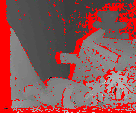
(a) BOX ($14.23\%$)

(b) NL ($8.60\%$)

(c) ST ($9.78\%$)

(d) BF ($10.24\%$)

(e) GF ($8.25\%$)

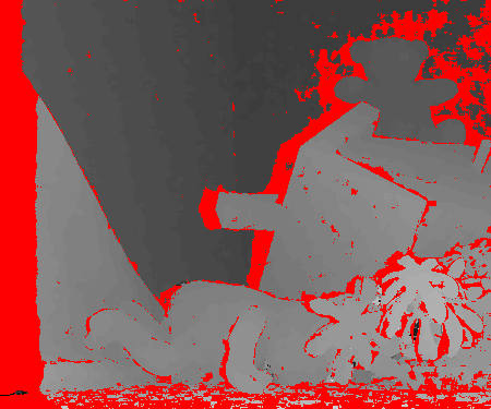
(f) S+BOX ($11.18\%$)

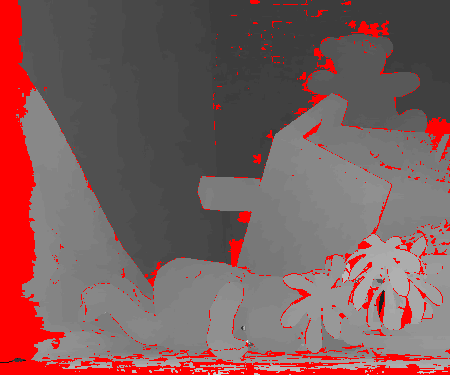
(g) S+NL ($5.74\%$)

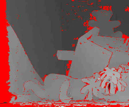
(h) S+ST ($6.22\%$)

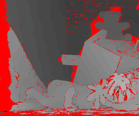
(i) S+BF ($8.17\%$)

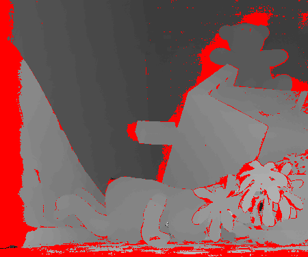
(j) S+GF ($6.99\%$)

Figure 4: Disparity maps of Teddy for all cost aggregation methods (with no disparity refinement techniques). The non-occ error rate is shown in each subtitle. Red pixels indicate erroneous pixels, where the absolute disparity error is larger than $1$. (Best viewed in color.)

In this section, we use Middlebury [23], KITTI [4] and New Tsukuba [20] datasets to validate that when integrating state-of-the-art cost aggregation methods, such as BF [36], GF [21], NL [33] and ST [16], into our framework, there will be significant performance improvements. Furthermore, we also implement the simple box filter aggregation method (named as BOX, window size is $7\times 7$) to serve as a baseline, which also becomes very powerful when integrated into our framework. For NL and ST, we directly use the C++ codes provided by the authors^,, and thus all the parameter settings are identical to those used in their implementations. For GF, we implemented our own C++ code by referring to the author-provided software (implemented in MATLAB) in order to process high-resolution images from KITTI and New Tsukuba datasets efficiently. For BF, we implemeted the asymmetric version as suggested by [9]. The local WTA strategy is adopted to generate a disparity map. In order to compare different cost aggregation methods fairly, no disparity refinement technique is employed, unless we explicitly declare. $S$ is set to 4, i.e. totally five scales are used in our framework. For the regularization parameter $\lambda$, we set it to $0.3$ for the Middlebury dataset, while setting it to $1.0$ on the KITTI and New Tsukuba datasets for more regularization, considering these two datasets contain a large portion of textureless regions.

6.1 Middlebury Dataset

The Middlebury benchmark [24] is a de facto standard for comparing existing stereo matching algorithms. In the benchmark [24], four stereo pairs (Tsukuba, Venus, Teddy, Cones) are used to rank more than $100$ stereo matching algorithms. In our experiment, we adopt these four stereo pairs. In addition, we use ‘Middlebury 2005’ [22] ($6$ stereo pairs) and ‘Middlebury 2006’ [8] ($21$ stereo pairs) datasets, which involve more complex scenes. Thus, we have $31$ stereo pairs in total, denoted as M31. It is worth mentioning that during our experiments, all local cost aggregation methods perform rather bad (error rate of non-occlusion (non-occ) area is more than $20\%$) in $4$ stereo pairs from Middlebury 2006 dataset, i.e. Midd1, Midd2, Monopoly and Plastic. A common property of these $4$ stereo pairs is that they all contain large textureless regions, making local stereo methods fragile. In order to alleviate bias towards these four stereo pairs, we exclude them from M31 to generate another collection of stereo pairs, which we call M27. We make statistics on both M31 and M27 (Table 1). We adopt the intensity + gradient cost function in Equation (2), which is widely used in state-of-the-art cost aggregation methods [21, 16, 33].

In Table 1, we show the average error rates of non-occ region for different cost aggregation methods on both M31 and M27 datasets. We use the prefix ‘S+’ to denote the integration of existing cost aggregation methods into cross-scale cost aggregation framework. Avg Non-occ is an average percentage of bad matching pixels in non-occ regions, where the absolute disparity error is larger than $1$. The results are encouraging: all cost aggregation methods see an improvement when using cross-scale cost aggregation, and even the simple BOX method becomes very powerful (comparable to state-of-the-art on M27) when using cross-scale cost aggregation. Disparity maps of Teddy stereo pair for all these methods are shown in Figure 4, while others are shown in the supplementary material due to space limit.

Furthermore, to follow the standard evaluation metric of the Middlebury benchmark [24], we show each cost aggregation method’s rank on the website (as of October 2013) in Table 1. Avg Rank and Avg Err indicate the average rank and error rate measured using Tsukuba, Venus, Teddy and Cones images [24]. Here each method is combined with the state-of-the-art disparity refinement technique from [33] (For ST [16], we list its original rank reported in the Middlebury benchmark [24], since the same results was not reproduced using the author’s C++ code). The rank also validates the effectiveness of our framework. We also reported the running time for Tsukuba stereo pair on a PC with a 2.83 GHz CPU and 8 GB of memory. As mentioned before, the computational overhead is relatively small. To be specific, it consists of the cost aggregation of $\mathbf{\tilde{C}}^{s}$ ($s\in\{0,1,\cdots,S\}$) and the computation of Equation (13).

Method	Avg Non-occ(%)		Avg	Avg	Time
	M31	M27	Rank	Err(%)	(s)
BOX	15.45	10.7	59.6	6.2	0.11
S+BOX	13.09	8.55	51.9	5.93	0.15
NL[33]	12.22	9.44	41.2	5.48	0.29
S+NL	11.49	8.73	39.4	5.2	0.37
ST[16]	11.52	8.95	31.6	5.35	0.2
S+ST	10.51	8.07	27.9	4.97	0.29
BF[36]	12.26	8.77	48.1	5.89	60.53
S+BF	10.95	8.04	40.7	5.56	70.62
GF[21]	10.5	6.84	40.5	5.64	1.16
S+GF	9.39	6.20	37.7	5.51	1.32

Table 1: Quantitative evaluation of cost aggregation methods on the Middlebury dataset. The prefix ‘S+’ denotes our cross-scale cost aggregation framework. For the rank part (column $4$ and $5$), the disparity results were refined with the same disparity refinement technique [33].

6.2 KITTI Dataset

Method	Out-Noc	Out-All	Avg-Noc	Avg-All
BOX	22.51 %	24.28 %	12.18 px	12.95 px
S+BOX	12.06 %	14.07 %	3.54 px	4.57 px
NL[33]	24.69 %	26.38 %	4.36 px	5.54 px
S+NL	25.41 %	27.08 %	4.00 px	5.20 px
ST[16]	24.09 %	25.81 %	4.31 px	5.47 px
S+ST	24.51 %	26.22 %	3.82 px	5.02 px
GF[21]	12.50 %	14.51 %	4.64 px	5.69 px
S+GF	9.66 %	11.73 %	2.19 px	3.36 px

Table 2: Quantitative comparison of cost aggregation methods on KITTI dataset. Out-Noc: percentage of erroneous pixels in non-occluded areas; Out-All: percentage of erroneous pixels in total; Avg-Noc: average disparity error in non-occluded areas; Avg-All: average disparity error in total.

The KITTI dataset [4] contains $194$ training image pairs and $195$ test image pairs for evaluating stereo matching algorithms. For the KITTI dataset, image pairs are captured under real-world illumination condition and almost all image pairs have a large portion of textureless regions, e.g. walls and roads [4]. During our experiment, we use the whole $194$ training image pairs with ground truth disparity maps available. The evaluation metric is the same as the KITTI benchmark [5] with an error threshold $3$. Besides, since BF is too slow for high resolution images (requiring more than one hour to process one stereo pair), we omit BF from evaluation.

Considering the illumination variation on the KITTI dataset, we adopt Census Transform [37], which is proved to be powerful for robust optical flow computation [6]. We show the performance of different methods when integrated into cross-scale cost aggregation in Table 2. Some interesting points are worth noting. Firstly, for BOX and GF, there are significant improvements when using cross-scale cost aggregation. Again, like the Middlebury dataset, the simple BOX method becomes very powerful by using cross-scale cost aggregation. However, for S+NL and S+ST, their performances are almost the same as those without cross-scale cost aggregation, which are even worse than that of S+BOX. This may be due to the non-local property of tree-based cost aggregation methods. For textureless slant planes, e.g. roads, tree-based methods tend to overuse the piecewise constancy assumption and may generate erroneous fronto-parallel planes. Thus, even though the cross-scale cost aggregation is adopted, errors in textureless slant planes are not fully addressed. Disparity maps for all methods are presented in the supplementary material, which also validate our analysis.

6.3 New Tsukuba Dataset

Method	Out-Noc	Out-All	Avg-Noc	Avg-All
BOX	31.08 %	37.70 %	7.37 px	10.72 px
S+BOX	18.82 %	26.50 %	3.92 px	7.44 px
NL[33]	21.88 %	26.72 %	4.12 px	6.40 px
S+NL	19.84 %	24.50 %	3.65 px	5.73 px
ST[16]	21.68 %	27.07 %	4.33 px	7.02 px
S+ST	18.99 %	24.16 %	3.60 px	5.96 px
GF[21]	23.42 %	30.34 %	6.35 px	9.86 px
S+GF	14.40 %	21.78 %	3.10 px	6.38 px

Table 3: Quantitative comparison of cost aggregation methods on New Tsukuba dataset.

The New Tsukuba Dataset [20] contains $1800$ stereo pairs with ground truth disparity maps. These pairs consist of a one minute photorealistic stereo video, generated by moving a stereo camera in a computer generated 3D scene. Besides, there are $4$ different illumination conditions: Daylight, Fluorescent, Lamps and Flashlight. In our experiments, we use the Daylight scene, which has a challenging real world illumination condition [20]. Since neighboring frames usually share similar scenes, we sample the $1800$ frames every second to get a subset of $60$ stereo pairs, which saves the evaluation time. We test both intensity + gradient and Census Transform cost functions, and intensity + gradient cost function gives better results in this dataset. Disparity level of this dataset is the same as the KITTI dataset, i.e. $256$ disparity levels, making BF [36] too slow, so we omit BF from evaluation.

Table 3 shows evaluation results for different cost aggregation methods on New Tsukuba dataset. We use the same evaluation metric as the KITTI benchmark [5] (error threshold is $3$). Again, all cost aggregation methods see an improvement when using cross-scale cost aggregation.

6.4 Regularization Parameter Study

Figure 5: The effect of varying inter-scale regularization parameter for different methods.

The key parameter in Equation (7) is the regularization parameter $\lambda$. By adjusting this parameter, we can control the strength of inter-scale regularization as shown in Figure 5. The error rate is evaluated on M31. When $\lambda$ is set to $0$, inter-scale regularization is prohibited, which is equivalent to performing cost aggregation at the finest scale. When regularization is introduced, there are improvements for all methods. As $\lambda$ becomes large, the regularization term dominates the optimization, causing the cost volume of each scale to be purely identical. As a result, fine details of disparity maps are missing and error rate increases. One may note that it will generate better results by choosing different $\lambda$ for different cost aggregation methods, though we use consistent $\lambda$ for all methods.

7 Conclusions and Future Work

In this paper, we have proposed a cross-scale cost aggregation framework for stereo matching. This paper is not intended to present a completely new cost aggregation method that yields a highly accurate disparity map. Rather, we investigate the scale space behavior of various cost aggregation methods. Extensive experiments on three datasets validated the effect of cross-scale cost aggregation. Almost all methods saw improvements and even the simple box filtering method combined with our framework achieved very good performance.

Recently, a new trend in stereo vision is to solve the correspondence problem in continuous plane parameter space rather than in discrete disparity label space [1, 13, 32]. These methods can handle slant planes very well and one probable future direction is to investigate the scale space behavior of these methods.

8 Acknowledgement

This work was supported by XXXXXXXXXXXX.

References

- [1] M. Bleyer, C. Rhemann, and C. Rother. PatchMatch stereo - stereo matching with slanted support windows. In BMVC, 2011.
- [2] P. J. Burt. Fast filter transform for image processing. CGIP, 1981.
- [3] P. Felzenszwalb and D. Huttenlocher. Efficient belief propagation for early vision. In CVPR, 2004.
- [4] A. Geiger, P. Lenz, and R. Urtasun. Are we ready for autonomous driving? The KITTI vision benchmark suite. In CVPR, 2012.
- [5] A. Geiger, P. Lenz, and R. Urtasun. The KITTI Vision Benchmark Suite. http://www.cvlibs.net/datasets/kitti/eval\_stereo\_flow.php?benchmark=stereo, 2012.
- [6] D. Hafner, O. Demetz, and J. Weickert. Why is the census transform good for robust optic flow computation? In SSVM, 2013.
- [7] K. He, J. Sun, and X. Tang. Guided image filtering. In ECCV, 2010.
- [8] H. Hirschmuller and D. Scharstein. Evaluation of cost functions for stereo matching. In CVPR, 2007.
- [9] A. Hosni, M. Bleyer, and M. Gelautz. Secrets of adaptive support weight techniques for local stereo matching. CVIU, 2013.
- [10] W. Hu, K. Zhang, L. Sun, and S. Yang. Comparisons reducing for local stereo matching using hierarchical structure. In ICME, 2013.
- [11] Y.-H. Jen, E. Dunn, P. Fite-Georgel, and J.-M. Frahm. Adaptive scale selection for hierarchical stereo. In BMVC, 2011.
- [12] C. Liu, J. Yuen, and A. Torralba. SIFT flow: dense correspondence across scenes and its applications. TPAMI, 2011.
- [13] J. Lu, H. Yang, D. Min, and M. N. Do. Patch match filter: efficient edge-aware filtering meets randomized search for fast correspondence field estimation. In CVPR, 2013.
- [14] H. A. Mallot, S. Gillner, and P. A. Arndt. Is correspondence search in human stereo vision a coarse-to-fine process? Biological Cybernetics, 1996.
- [15] D. Marr and T. Poggio. A computational theory of human stereo vision. Proceedings of the Royal Society of London. Series B. Biological Sciences, 1979.
- [16] X. Mei, X. Sun, W. Dong, H. Wang, and X. Zhang. Segment-tree based cost aggregation for stereo matching. In CVPR, 2013.
- [17] M. D. Menz and R. D. Freeman. Stereoscopic depth processing in the visual cortex: a coarse-to-fine mechanism. Nature neuroscience, 2003.
- [18] P. Milanfar. A tour of modern image filtering: new insights and methods, both practical and theoretical. IEEE Signal Processing Magazine, 2013.
- [19] D. Min and K. Sohn. Cost aggregation and occlusion handling with WLS in stereo matching. TIP, 2008.
- [20] M. Peris, A. Maki, S. Martull, Y. Ohkawa, and K. Fukui. Towards a simulation driven stereo vision system. In ICPR, 2012.
- [21] C. Rhemann, A. Hosni, M. Bleyer, C. Rother, and M. Gelautz. Fast cost-volume filtering for visual correspondence and beyond. In CVPR, 2011.
- [22] D. Scharstein and C. Pal. Learning conditional random fields for stereo. In CVPR, 2007.
- [23] D. Scharstein and R. Szeliski. A taxonomy and evaluation of dense two-frame stereo correspondence algorithms. IJCV, 2002.
- [24] D. Scharstein and R. Szeliski. Middlebury Stereo Vision Website. http://vision.middlebury.edu/stereo/, 2002.
- [25] H. Simon and K. Reinhard. Evaluation of a new coarse-to-fine strategy for fast semi-global stereo matching. Advances in Image and Video Technology, 2012.
- [26] M. Sizintsev. Hierarchical stereo with thin structures and transparency. In CCCRV, 2008.
- [27] L. Tang, M. K. Garvin, K. Lee, W. L. M. Alward, Y. H. Kwon, and M. D. Abràmoff. Robust multiscale stereo matching from fundus images with radiometric differences. TPAMI, 2011.
- [28] C. Tomasi and R. Manduchi. Bilateral filtering for gray and color images. In ICCV, 1998.
- [29] F. Tombari, S. Mattoccia, L. Di Stefano, and E. Addimanda. Classification and evaluation of cost aggregation methods for stereo correspondence. In CVPR, 2008.
- [30] G. Van Meerbergen, M. Vergauwen, M. Pollefeys, and L. Van Gool. A hierarchical symmetric stereo algorithm using dynamic programming. IJCV, 2002.
- [31] Z.-F. Wang and Z.-G. Zheng. A region based stereo matching algorithm using cooperative optimization. In CVPR, 2008.
- [32] K. Yamaguchi, D. McAllester, and R. Urtasun. Robust monocular epipolar flow estimation. In CVPR, 2013.
- [33] Q. Yang. A non-local cost aggregation method for stereo matching. In CVPR, 2012.
- [34] Q. Yang, L. Wang, R. Yang, H. Stewénius, and D. Nistér. Stereo matching with color-weighted correlation, hierarchical belief propagation, and occlusion handling. TPAMI, 2009.
- [35] R. Yang and M. Pollefeys. Multi-resolution real-time stereo on commodity graphics hardware. In CVPR, 2003.
- [36] K.-J. Yoon and I. S. Kweon. Adaptive support-weight approach for correspondence search. TPAMI, 2006.
- [37] R. Zabih and J. Woodfill. Non-parametric local transforms for computing visual correspondence. In ECCV, 1994.