A SPACE-TIME FEM FOR PDES ON EVOLVING SURFACES

Abstract

The paper studies a finite element method for computing transport and diffusion along evolving surfaces. The method does not require a parametrization of a surface or an extension of a PDE from a surface into a bulk outer domain. The surface and its evolution may be given implicitly, e.g., as the solution of a level set equation. This approach naturally allows a surface to undergo topological changes and experience local geometric singularities. The numerical method uses space-time finite elements and is provably second order accurate. The paper reviews the method, error estimates and shows results for computing the diffusion of a surfactant on surfaces of two colliding droplets.

J. Grande, M.A. Olshanskii and A. Reusken

1 INTRODUCTION

Partial differential equations posed on evolving surfaces appear in a number of applications. Recently, several numerical approaches for handling such type of problems have been introduced, cf. [1]. In [2, 3] Dziuk and Elliott developed and analyzed a finite element method for computing transport and diffusion on a surface which is based on a Lagrangian tracking of the surface evolution. Methods using an Eulerian approach were developed in [4, 5, 6], based on an extension of the surface PDE into a bulk domain that contains the surface. Recently, in [7, 8, 9] another Eulerian method, which does not use an extension of the PDE into the bulk domain, has been introduced and analyzed. The key idea of this method is to use restrictions of (usual) space-time volumetric finite element functions to the space-time manifold. This trace finite element technique has been studied for stationary surfaces in [10, 11, 12].

In this paper we summarize the key ideas of this space-time trace-FEM and some main results of the error analysis, in particular a result on second order accuracy of the method in space and time. For details we refer to [7, 9]. In the numerical experiments in [7, 8, 9] only relatively simple model problems with smoothly evolving surfaces are considered. As a new contribution in this paper we present results of a numerical experiment for a surfactant transport equation on an evolving manifold with a topological singularity, which resembles a droplet collision. The method that we study uses volumetric finite element spaces which are continuous piecewise linear in space and discontinuous piecewise linear in time. This allows a natural time-marching procedure, in which the numerical approximation is computed on one time slab after another. Spatial triangulations may vary per time slab. The results of the numerical experiment show that the method is extremely robust and that even for the case with a topological singularity (droplet collision) accurate results can be obtained on a fixed Eulerian (space-time) grid with a large time step.

As a model problem we use the following one. Consider a surface $\Gamma(t)$ passively advected by a given smooth velocity field $\mathbf{w}=\mathbf{w}(x,t)$, i.e. the normal velocity of $\Gamma(t)$ is given by $\mathbf{w}\cdot\mathbf{n}$, with $\mathbf{n}$ the unit normal on $\Gamma(t)$. We assume that for all $t\in[0,T]$, $\Gamma(t)$ is a hypersurface that is closed ($\partial\Gamma=\emptyset$), connected, oriented, and contained in a fixed domain $\Omega\subset\mathbb{R}^{d}$, $d=2,3$. In the remainder we consider $d=3$, but all results have analogs for the case $d=2$. The convection-diffusion equation on the surface that we consider is given by:

$$\dot{u}+({\mathop{\rm div}}_{\Gamma}\mathbf{w})u-{\nu_{d}}\Delta_{\Gamma}u=f\qquad\text{on}~{}~{}\Gamma(t),~{}~{}t\in(0,T],$$ (1)

with a prescribed source term $f=f(x,t)$ and homogeneous initial condition $u(x,0)=u_{0}(x)=0$ for $x\in\Gamma_{0}:=\Gamma(0)$. Here $\dot{u}=\frac{\partial u}{\partial t}+\mathbf{w}\cdot\nabla u$ denotes the advective material derivative, ${\mathop{\rm div}}_{\Gamma}:=\operatorname{tr}\left((I-\mathbf{n}\mathbf{n}^{T})\nabla\right)$ is the surface divergence and $\Delta_{\Gamma}$ is the Laplace-Beltrami operator, $\nu_{d}>0$ is the constant diffusion coefficient. If we take $f=0$ and an initial condition $u_{0}\neq 0$, this surface PDE is obtained from mass conservation of the scalar quantity $u$ with a diffusive flux on $\Gamma(t)$ (cf. [13, 14]). A standard transformation to a homogeneous initial condition, which is convenient for a theoretical analysis, leads to (1).

2 WELL-POSED SPACE-TIME WEAK FORMULATION

Several weak formulations of (1) are known in the literature, see [2, 14]. The most appropriate for our purposes is a integral space-time formulation proposed in [7]. In this section we outline this formulation. Consider the space-time manifold

$$\mathcal{S}=\bigcup\limits_{t\in(0,T)}\Gamma(t)\times\{t\},\quad\mathcal{S}\subset\mathbb{R}^{4}.$$

On $L^{2}(\mathcal{S})$ we use the scalar product $(v,w)_{0}=\int_{0}^{T}\int_{\Gamma(t)}vw\,ds\,dt$. Let $\nabla_{\Gamma}$ denote the tangential gradient for $\Gamma(t)$ and introduce the space

$$H=\{\,v\in L^{2}(\mathcal{S})~{}|~{}\|\nabla_{\Gamma}v\|_{L^{2}(\mathcal{S})}<\infty\,\}$$

endowed with the scalar product

$$(u,v)_{H}=(u,v)_{0}+(\nabla_{\Gamma}u,\nabla_{\Gamma}v)_{0}.$$ (2)

We consider the material derivative $\dot{u}$ of $u\in H$ as a distribution on $\mathcal{S}$:

$$\left\langle\dot{u},\phi\right\rangle=-\int_{0}^{T}\int_{\Gamma(t)}u\dot{\phi}+u\phi{\,\operatorname{div_{\Gamma}}}\mathbf{w}\,ds\,dt\quad\text{for all}~{}~{}\phi\in C_{0}^{1}(\mathcal{S}).$$

In [7] it is shown that $C_{0}^{1}(\mathcal{S})$ is dense in $H$. If $\dot{u}$ can be extended to a bounded linear functional on $H$, we write $\dot{u}\in H^{\prime}$. Define the space

$$W=\{\,u\in H~{}|~{}\dot{u}\in H^{\prime}\,\},\quad\text{with}~{}~{}\|u\|_{W}^{2}:=\|u\|_{H}^{2}+\|\dot{u}\|_{H^{\prime}}^{2}.$$

In [7] properties of $H$ and $W$ are derived. Both spaces are Hilbert spaces and smooth functions are dense in $H$ and $W$. Define

$$\overset{\circ}{W}:=\{\,v\in W~{}|~{}v(\cdot,0)=0\quad\text{on}~{}\Gamma_{0}\,\}.$$

The space $\overset{\circ}{W}$ is well-defined, since functions from $W$ have well-defined traces in $L^{2}(\Gamma(t))$ for any $t\in[0,T]$. We introduce the symmetric bilinear form

$$a(u,v)=\nu_{d}(\nabla_{\Gamma}u,\nabla_{\Gamma}v)_{0}+({\,\operatorname{div_{\Gamma}}}\mathbf{w}\,u,v)_{0},\quad u,v\in H,$$

which is continuous on $H\times H$:

$$a(u,v)\leq(\nu_{d}+\alpha_{\infty})\|u\|_{H}\|v\|_{H},\quad\text{with}~{}\alpha_{\infty}:=\|{\,\operatorname{div_{\Gamma}}}\mathbf{w}\|_{L^{\infty}(\mathcal{S})}.$$

The weak space-time formulation of (1) reads: For given $f\in L^{2}(\mathcal{S})$ find $u\in\overset{\circ}{W}$ such that

$$\left\langle\dot{u},v\right\rangle+a(u,v)=(f,v)_{0}\quad\text{for all}~{}~{}v\in H.$$ (3)

In [7] the inf-sup property

$$\inf_{0\neq u\in\overset{\circ}{W}}~{}\sup_{0\neq v\in\overset{\phantom{.}}{H}}\frac{\left\langle\dot{u},v\right\rangle+a(u,v)}{\|u\|_{W}\|v\|_{H}}\geq c_{s}>0$$ (4)

is proved. Using this in combination with the continuity result one can show that the weak formulation (3) is well-posed.

We introduce a similar “time-discontinuous” weak formulation that is better suited for the finite element method that we consider. We take a partitioning of the time interval: $0=t_{0}<t_{1}<\ldots<t_{N}=T$, with a uniform time step $\Delta t=T/N$. The assumption of a uniform time step is made to simplify the presentation, but is not essential. A time interval is denoted by $I_{n}:=(t_{n-1},t_{n}]$. The symbol $\mathcal{S}^{n}$ denotes the space-time interface corresponding to $I_{n}$, i.e., $\mathcal{S}^{n}:=\cup_{t\in I_{n}}\Gamma(t)\times\{t\}$, and $\mathcal{S}:=\cup_{1\leq n\leq N}\mathcal{S}^{n}$. We introduce the following subspaces of $H$:

$$H_{n}:=\{\,v\in H~{}|~{}v=0\quad\text{on}~{}~{}\mathcal{S}\setminus\mathcal{S}^{n}\,\},$$

and define the spaces

$$W_{n} =\{\,v\in H_{n}~{}|~{}\dot{v}\in H_{n}^{\prime}\,\},\quad\|v\|_{W_{n}}^{2}=\|v\|_{H}^{2}+\|\dot{v}\|_{H_{n}^{\prime}}^{2},$$ (5)

$$W^{b} :=\oplus_{n=1}^{N}W_{n},~{}~{}\text{with norm}~{}~{}\|v\|_{W^{b}}^{2}=\sum_{n=1}^{N}\|v\|_{W_{n}}^{2}.$$ (6)

For $u\in W_{n}$, the one-sided limits $u_{+}^{n}=u_{+}(\cdot,t_{n})$ (i.e., $t\downarrow t_{n}$) and ${u}_{-}^{n}=u_{-}(\cdot,t_{n})$ (i.e., $t\uparrow t_{n}$) are well-defined in $L^{2}(\Gamma(t_{n}))$. At $t_{0}$ and $t_{N}$ only $u_{+}^{0}$ and $u_{-}^{N}$ are defined. For $v\in W^{b}$, a jump operator is defined by $[v]^{n}=v_{+}^{n}-v_{-}^{n}\in L^{2}(\Gamma(t_{n}))$, $n=1,\dots,N-1$. For $n=0$, we define $[v]^{0}=v_{+}^{0}$. On the cross sections $\Gamma(t_{n})$, $0\leq n\leq N$, of $\mathcal{S}$ the $L^{2}$ scalar product is denoted by

$$(\psi,\phi)_{t_{n}}:=\int_{\Gamma(t_{n})}\psi\phi\,ds.$$

In addition to $a(\cdot,\cdot)$, we define on the broken space $W^{b}$ the following bilinear forms:

$$d(u,v)=\sum_{n=1}^{N}d^{n}(u,v),\quad d^{n}(u,v)=([u]^{n-1},v_{+}^{n-1})_{t_{n-1}},\quad\left\langle\dot{u},v\right\rangle_{b}=\sum_{n=1}^{N}\left\langle\dot{u}_{n},v_{n}\right\rangle.$$

One can show that the unique solution to (3) is also the unique solution of the following variational problem in the broken space: Find $u\in W^{b}$ such that

$$\left\langle\dot{u},v\right\rangle_{b}+a(u,v)+d(u,v)=(f,v)_{0}\quad\text{for all}~{}~{}v\in W^{b}.$$ (7)

For this time discontinuous weak formulation an inf-sup stability result (that is weaker than the one in (4)) can be derived. The variational formulation uses $W^{b}$, instead of $H$, as test space, since the term $d(u,v)$ is not well-defined for an arbitrary $v\in H$. Also note that the initial condition $u(\cdot,0)=0$ is not an essential condition in the space $W^{b}$ but is treated in a weak sense (as is standard in DG methods for time dependent problems). From an algorithmic point of view the formulation (7) has the advantage that due to the use of the broken space $W^{b}=\oplus_{n=1}^{N}W_{n}$ it can be solved in a time stepping manner.

3 SPACE-TIME FINITE ELEMENT METHOD

We introduce a finite element method which is a Galerkin method with $W_{h}\subset W^{b}$ applied to the variational formulation (7). To define this $W_{h}$, consider the partitioning of the space-time volume domain $Q=\Omega\times(0,T]\subset\mathbb{R}^{3+1}$ into time slabs $Q_{n}:=\Omega\times I_{n}$. Corresponding to each time interval $I_{n}:=(t_{n-1},t_{n}]$ we assume a given shape regular tetrahedral triangulation $\mathcal{T}_{n}$ of the spatial domain $\Omega$. The corresponding spatial mesh size parameter is denoted by $h$. Then $\mathcal{Q}_{h}=\bigcup\limits_{n=1,\dots,N}\mathcal{T}_{n}\times I_{n}$ is a subdivision of $Q$ into space-time prismatic nonintersecting elements. We shall call $\mathcal{Q}_{h}$ a space-time triangulation of $Q$. Note that this triangulation is not necessarily fitted to the surface $\mathcal{S}$. We allow $\mathcal{T}_{n}$ to vary with $n$ (in practice, during time integration one may wish to adapt the space triangulation depending on the changing local geometric properties of the surface) and so the elements of $\mathcal{Q}_{h}$ may not match at $t=t_{n}$.

For any $n\in\{1,\dots,N\}$, let $V_{n}$ be the finite element space of continuous piecewise linear functions on $\mathcal{T}_{n}$. We define the volume space-time finite element space:

$$V_{h}:=\{\,v:Q\to\mathbb{R}~{}|~{}v(x,t)=\phi_{0}(x)+t\phi_{1}(x)~{}\text{on every}~{}Q_{n},~{}\text{with}~{}\phi_{0},\,\phi_{1}\in V_{n}\,\}.$$ (8)

Thus, $V_{h}$ is a space of piecewise P1 functions with respect to $\mathcal{Q}_{h}$, continuous in space and discontinuous in time. Now we define our surface finite element space as the space of traces of functions from $V_{h}$ on $\mathcal{S}$:

$$W_{h}:=\{\,w:\mathcal{S}\to\mathbb{R}~{}|~{}w=v_{|\mathcal{S}},~{}~{}v\in V_{h}\,\}.$$ (9)

The finite element method reads: Find $u_{h}\in W_{h}$ such that

$$\left\langle\dot{u}_{h},v_{h}\right\rangle_{b}+a(u_{h},v_{h})+d(u_{h},v_{h})=(f,v_{h})_{0}\quad\text{for all}~{}~{}v_{h}\in W_{h}.$$ (10)

As usual in time-DG methods, the initial condition for $u_{h}(\cdot,0)$ is treated in a weak sense. Due to $u_{h}\in H^{1}(Q_{n})$ for all $n=1,\dots,N$, the first term in (10) can be written as

$$\left\langle\dot{u}_{h},v_{h}\right\rangle_{b}=\sum_{n=1}^{N}\int_{t_{n-1}}^{t_{n}}\int_{\Gamma(t)}(\frac{\partial u_{h}}{\partial t}+\mathbf{w}\cdot\nabla u_{h})v_{h}ds\,dt.$$

The method can be implemented with a time marching strategy. Of course, for the implementation of the method one needs a quadrature rule to approximate the integrals over $\mathcal{S}^{n}$. This issue is briefly addressed in Section 5.

4 DISCRETIZATION ERROR ANALYSIS

In this section we briefly address the discretization error analysis of the method (10), which is presented in [9]. We first explain a discrete mass conservation property of the scheme (10). We consider the case that (1) is derived from mass conservation of a scalar quantity with a diffusive flux on $\Gamma(t)$. The original problem then has a nonzero initial condition $u_{0}$ and a source term $f\equiv 0$. The solution $u$ of the original problem has the mass conservation property $\bar{u}(t):=\int_{\Gamma(t)}u\,ds=\int_{\Gamma(0)}u_{0}\,ds$ for all $t\in[0,T]$. After a suitable transformation one obtains the equation (1) with a zero initial condition $u_{0}$ and a right hand-side $f$ which satisfies $\int_{\Gamma(t)}f\,ds=0$ for all $t\in[0,T]$. The solution $u$ of (1) then has the “shifted” mass conservation property $\bar{u}(t)=0$ for all $t\in[0,T]$. Tak ing suitable test functions in the discrete problem (10) we obtain that the discrete solution $u_{h}$ has the following weaker mass conservation property, with $\bar{u}_{h}(t):=\int_{\Gamma(t)}u_{h}\,ds$:

$$\bar{u}_{h,-}(t_{n})=0\quad\text{and}\quad\int_{t_{n-1}}^{t_{n}}\bar{u}_{h}(t)\,dt=0,\quad n=1,2,\dots N.$$ (11)

For a stationary surface, $\bar{u}_{h}(t)$ is a piecewise affine function and thus (11) implies $\bar{u}_{h}(t)\equiv 0$, i.e,. we have exact mass conservation on the discrete level. If the surface evolves, the finite element method is not necessarily mass conserving: (11) holds, but $\bar{u}_{h}(t)\neq 0$ may occur for $t_{n-1}\leq t<t_{n}$. In the discretization error analysis we use a consistent stabilizing term involving the quantity $\bar{u}_{h}(t)$. More precisely, define

$$a_{\sigma}(u,v):=a(u,v)+\sigma\int_{0}^{T}\bar{u}(t)\bar{v}(t)\,dt,\quad\sigma\geq 0.$$ (12)

Instead of (10) we consider the stabilized version: Find $u_{h}\in W_{h}$ such that

$$\left\langle\dot{u}_{h},v_{h}\right\rangle_{b}+a_{\sigma}(u_{h},v_{h})+d(u_{h},v_{h})=(f,v_{h})_{0}\quad\text{for all}~{}~{}v_{h}\in W_{h}.$$ (13)

Taking $\sigma>0$ we expect both a stabilizing effect and an improved discrete mass conservation property. Ellipticity of finite element method bilinear form and error bounds are derived in the mesh-dependent norm:

$$|\!|\!|u|\!|\!|_{h}:=\left(\|u_{-}^{N}\|_{T}^{2}+\sum_{n=1}^{N}\|[u]^{n-1}\|_{t_{n-1}}^{2}+\|u\|_{H}^{2}\right)^{\frac{1}{2}}.$$

In the error analysis we need a condition which plays a similar role as the condition “$c-\frac{1}{2}\mathop{\rm div}b>0$” used in standard analyses of variational formulations of the convection-diffusion equation $-\Delta u+b\cdot\nabla u+cu=f$ in an Euclidean domain $\Omega\subset\mathbb{R}^{n}$, cf. [15]. This condition is as follows: there exists a $c_{0}>0$ such that

$${\,\operatorname{div_{\Gamma}}}\mathbf{w}(x,t)+\nu_{d}c_{F}(t)\geq c_{0}\quad\text{for all}~{}~{}x\in\Gamma(t),~{}t\in[0,T].$$ (14)

Here $c_{F}(t)>0$ results from the Poincare inequality

$$\int_{\Gamma(t)}|\nabla_{\Gamma}u|^{2}\,ds\geq c_{F}(t)\int_{\Gamma(t)}(u-\frac{1}{|\Gamma(t)|}\bar{u})^{2}\,ds\quad\forall~{}t\in[0,T],~{}~{}\forall~{}u\in H.$$ (15)

A main result derived in [9] is given in the following theorem. We assume that the time step $\Delta t$ and the spatial mesh size parameter $h$ have comparable size: $\Delta t\sim h$.
Theorem 1. Assume (14) and take $\sigma\geq\frac{\nu_{d}}{2}\max\limits_{t\in[0,T]}\frac{c_{F}(t)}{|\Gamma(t)|}$, where $c_{F}(t)$ is defined in (15). Then the ellipticity estimate

$$\left\langle\dot{u},u\right\rangle_{b}+a_{\sigma}(u,u)+d(u,u)\geq c_{s}|\!|\!|u|\!|\!|_{h}^{2}\quad\text{for all}~{}~{}u\in W^{b}$$ (16)

holds, with $c_{s}=\frac{1}{2}\min\{1,\nu_{d},c_{0}\}$ and $c_{0}$ from (14). Let $u\in\overset{\circ}{W}$ be the solution of (3) and assume $u\in H^{2}(\mathcal{S})$. For the solution $u_{h}\in W_{h}$ of the discrete problem (13) the following error bound holds:

$$|\!|\!|u-u_{h}|\!|\!|_{h}\leq ch\|u\|_{H^{2}(\mathcal{S})}.$$

A further main result derived in [9] is related to second order convergence. Denote by $\|\cdot\|_{-1}$ the norm dual to the $H^{1}_{0}(\mathcal{S})$ norm with respect to the $L^{2}$-duality. Under the conditions given in Theorem 1 and some further mild assumptions the error bound

$$\|u-u_{h}\|_{-1}\leq ch^{2}\|u\|_{H^{2}(\mathcal{S})}$$

holds. This second order convergence is derived in a norm weaker than the commonly considered $L^{2}(\mathcal{S})$ norm. The reason is that our arguments use isotropic polynomial interpolation error bounds on 4D space-time elements. Naturally, such bounds call for isotropic space-time $H^{2}$-regularity bounds for the solution. For our problem class such regularity is more restrictive than in an elliptic case, since the solution is generally less regular in time than in space. We can overcome this by measuring the error in the weaker $\|\cdot\|_{-1}$-norm.

5 NUMERICAL EXPERIMENT

In [7, 8] results of numerical experiments are presented. The examples considered there have smoothly evolving surfaces (e.g. a shrinking sphere) and the results show a convergence of order 1 in an $L^{2}(H^{1})$-norm (i.e. $L^{2}$ w.r.t time and $H^{1}$ w.r.t space) and of order 2 in an $L^{\infty}(L^{2})$ norm. This convergence behavior occurs already on relatively coarse meshes and there is no (CFL-type) condition on $\Delta t$.

In the example in this paper we consider an evolving surface $\Gamma(t)$ which undergoes a change of topology and experiences a local singularity. The computational domain is $x\in\Omega=(-3,3)\times(-2,2)^{2}$, $t\in[0,1]$. For representation of the evolving surface we use a level set function $\phi$ defined as:

$$\phi(x,t)=1-\frac{1}{\|x-c_{+}(t)\|^{3}}-\frac{1}{\|x-c_{-}(t)\|^{3}},$$

with $c_{\pm}(t)=\pm\frac{3}{2}(t-1,0,0)^{T}$. The surface $\Gamma(t)$ is defined as the zero level of $\phi(x,t)$, $t\in[0,1]$. Take $t=0$. Then for $x\in B(c_{+}(0);1)$ we have $\|x-c_{+}(0)\|^{-3}=1$ and $\|x-c_{-}(0)\|^{-3}\ll 1$. For $x\in B(c_{-}(0);1)$ we have $\|x-c_{+}(0)\|^{-3}\ll 1$ and $\|x-c_{-}(0)\|^{-3}=1$. Hence, the initial configuration $\Gamma(0)$ is (very) close to two balls of radius $1$, centered at $\pm(1.5,0,0)^{T}$. For $t=1$ the surface $\Gamma(1)$ is the ball around $0$ with radius $2^{1/3}$. For $t>0$ the two spheres approach each other until time $\tilde{t}=1-\tfrac{2}{3}2^{1/3}\approx 0.160$, when they touch at the origin. For $t\in(\tilde{t},1]$ the surface $\Gamma(t)$ is simply connected and smoothly deforms into the sphere $\Gamma(1)$.

In the vicinity of $\Gamma(t)$, the gradient $\nabla\phi$ and the time derivative $\partial_{t}\phi$ are well-defined and given by simple algebraic expressions. We construct the normal wind field, which transports $\Gamma(t)$, by inserting the ansatz $\mathbf{w}(x,t)=\alpha(x,t)\nabla\phi(x,t)$ into the level set equation $\partial_{t}\phi+\mathbf{w}\cdot\nabla\phi=0$. This yields

$$\mathbf{w}=-\frac{\partial_{t}\phi}{\lvert\nabla\phi\rvert^{2}}\nabla\phi.$$

We consider the surfactant advection-diffusion equation

$$\begin{cases}\dot{u}+\operatorname{div}_{\Gamma}\mathbf{w}\,u-\Delta_{\Gamma}u=0&\text{on }\Gamma(t),~{}t\in(0,1],\\ u(\cdot,0)=u_{0}&\text{on }\Gamma(0).\end{cases}$$ (17)

The initial surfactant distribution is given by

$$u_{0}(x)=\begin{cases}3-x_{1}&\text{for }x_{1}\geq 0,\\ 0&\text{else}.\end{cases}$$

The initial configuration is illustrated in Figure 1.

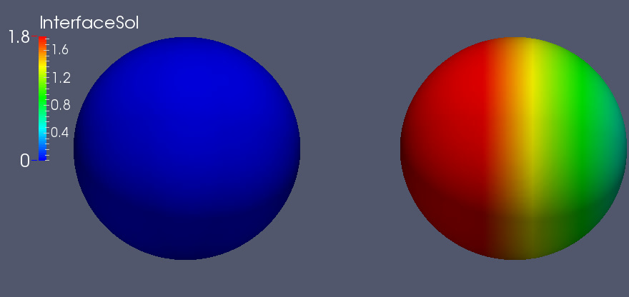
Figure 1: Initial condition as color on the initial zero level $\Gamma(0)$.

For the construction of a volume space-time finite element space we proceed as follows. On $\Omega$ we start with a level $l=0$ Kuhn-triangulation with mesh width $h_{0}=2$. We use regular refinement in the vicinity of the interface $\Gamma(t)$ to ensure that the interface is embedded in tetrahedra with refinement level $l\geq 1$. These tetrahedra have the mesh width $h_{l}=2^{1-l}$. On each time slab a level $l$ triangulation is used to define the volume space-time finite element space as in (8). For simplicity we use the same value for $l$ on all time slabs. The outer space induces a surface finite element space $W_{h}$ as in (9). This space is used for a Galerkin discretization of (17), as given in (10) (note that in this experiment we take $f=0$ and a nonhomogeneous initial condition $u_{0}$).

We outline the quadrature method for the approximation of integrals over $\mathcal{S}^{n}$. More details are given in [8]. Consider a single space-time prism $T\times I_{n}$ that is intersected by the space time manifold $\mathcal{S}^{n}$. Here $T$ is a level $l$ tetrahedron from the spatial triangulation. First $T$ is regularly refined into 8 tetrahedra $T_{j}$, $j=1,\ldots,8$. Each of the resulting space-time prisms $T_{j}\times I_{n}$ is partitioned into 4 pentatopes by inserting adequate diagonals. On each of these pentatopes the linear interpolant (in $\mathbb{R}^{4}$) of the level set function $\phi$ is computed. The zero level of this interpolant is (if not degenerated) a 3-dimensional convex polytope, which can be partitioned into tetrahedra. On these tetrahedra standard quadrature rules can be used. Note that in this approximation procedure we have a geometric error due to the approximation of the zero level of $\phi$ (which is the surface) by the zero level of its linear interpolant. This assembling procedure is completely local and can be done prism per prism.

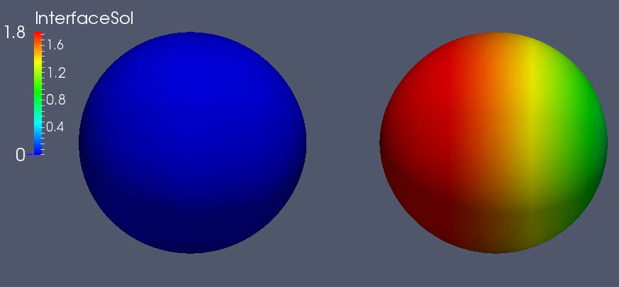
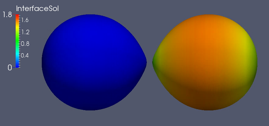
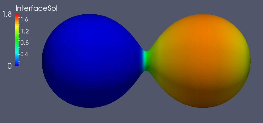
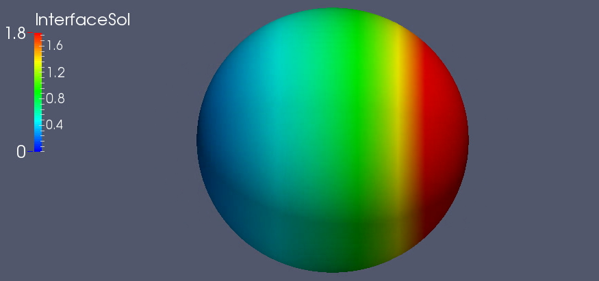
Figure 2: Snapshots of discrete solution, $l=5$, $\Delta t=2^{-7}$.

We present some results of numerical experiments. In Figure 2 we show a few snapshots of the surface and the computed surfactant distribution on a relatively fine space-time mesh, namely level $l=5$ and $\Delta t=2^{-7}$. As a measure of accuracy we computed the discrete mass on the space-time manifold:

$$I_{l,dt}(t_{n})=\int_{\Gamma_{h}(t_{n})}u\,d\sigma,\quad n=0,1,\ldots,N.$$

where $\Gamma_{h}(t_{n})$ is the approximation of $\Gamma(t_{n})$ obtained as zero level of the piecewise linear interpolant of $\phi$, cf. explanation above.
For $l=5$, $\Delta t=1/128$ the result is shown in Figure 3. We interpolated the values $I_{l,dt}(t_{n})$, $n=0,\ldots,N$, resulting in the discrete mass quantity as a function of $t\in[0,1]$. There is a mass loss of about $0.018$, which corresponds to a relative error of $\sim~{}9\cdot 10^{-4}$.

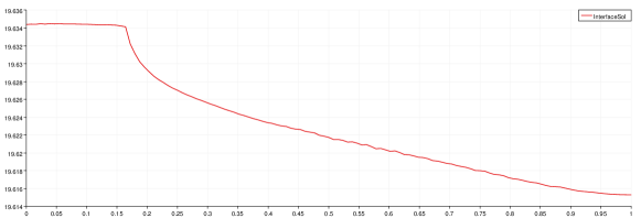
Figure 3: The total amount of surfactant $I_{5,1/128}$ over time.

In Figure 4 we show the result for $l=4$, $\Delta t=1/64$. The mass loss is $\sim~{}0.065$, which is about a factor $3.6$ more than for the case $l=5$, $\Delta t=1/128$.

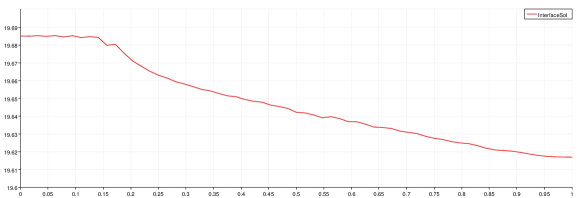
Figure 4: The total amount of surfactant $I_{4,1/64}$ over time.

Finally, we show result for level $l=4$, but with a large time step size $\Delta t=1/4$, i.e. we use use only four time steps to approximate the solution at $t=1$. The four discrete solutions at $t=0.25,0.5,0.75,1.0$ are shown in Figure 5. The total amount of surfactant is shown in Figure 6.

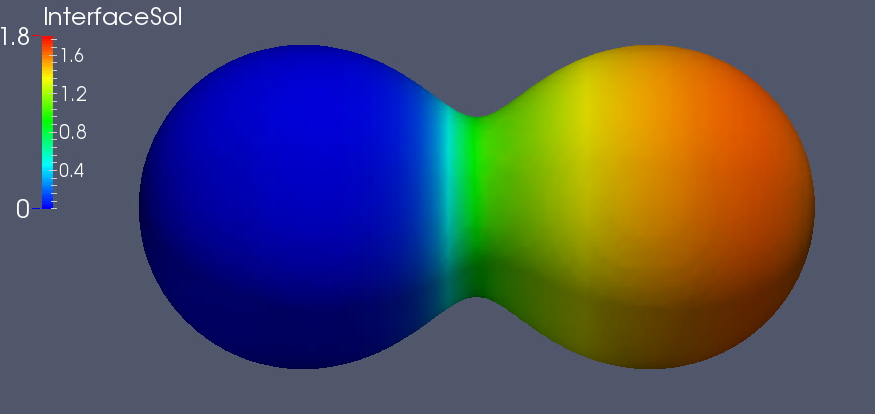
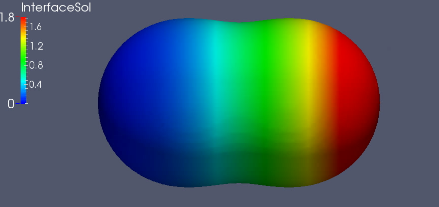
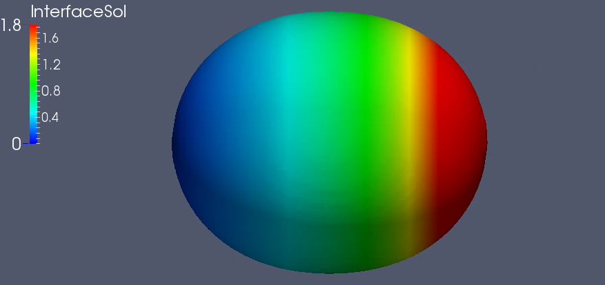
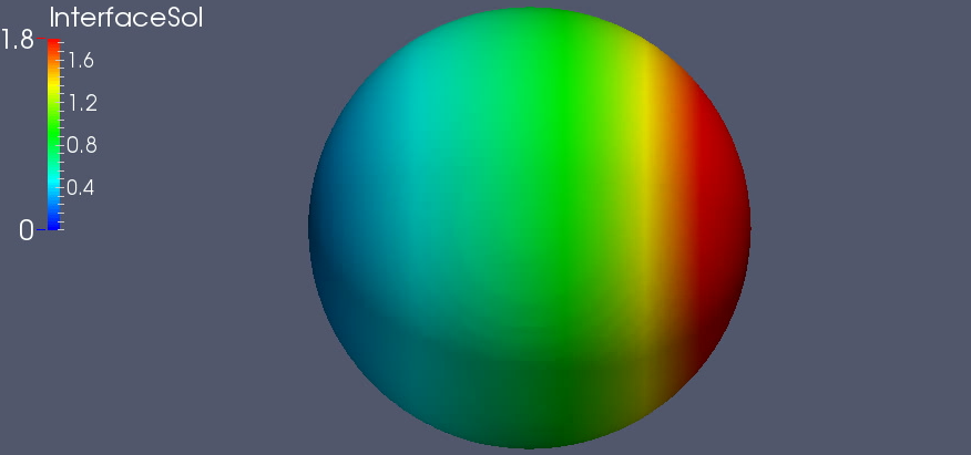
Figure 5: Snapshots of discrete solution, $l=4$, $\Delta t=\frac{1}{4}$, at $t=0.25,0.5,0.75,1$.

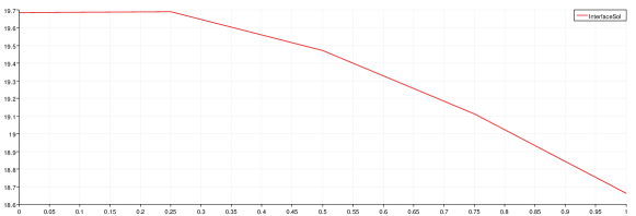
Figure 6: The total amount of surfactant $I_{4,1/4}$ over time.

6 DISCUSSION

We presented a space-time finite element method for solving PDEs on evolving surfaces. The method is based on traces of outer finite element spaces, is Eulerian in the sense that $\Gamma(t)$ is not tracked by a mesh, and can easily be combined with both space and time adaptivity. No extension of the equation away from the surface is needed and thus the number of d.o.f. involved in computations is optimal and comparable to methods in which $\Gamma$ is meshed directly. The computations are done in a time-marching manner as common for parabolic equations.

The method has second order convergence in space and time and conserves the mass in a weak sense, cf. (11). In practice, an artificial mass flux can be experienced due to geometric errors resulting from the approximation of $\Gamma(t)$. In experiments, the loss of mass was found to be small and quickly vanishing if the mesh is refined.

The implicit definition of the surface evolution with the help of a level set function is well suited for numerical treatment of surfaces which undergo topological changes and experience singularities. This report shows that the present space-time surface finite element method perfectly complements this property and provides a robust technique for computing diffusion and transport along colliding surfaces.

References

- [1] G. Dziuk and C. M. Elliott. Finite element methods for surface pdes. Acta Numerica, 22:289–396, 2013.
- [2] G. Dziuk and C. Elliott. Finite elements on evolving surfaces. IMA J. Numer. Anal., 27:262–292, 2007.
- [3] G. Dziuk and Ch. M. Elliott. -estimates for the evolving surface finite element method. Mathematics of Computation, 82:1–24, 2013.
- [4] D. Adalsteinsson and J. A. Sethian. Transport and diffusion of material quantities on propagating interfaces via level set methods. J. Comput. Phys., 185:271–288, 2003.
- [5] G. Dziuk and C. Elliott. An eulerian approach to transport and diffusion on evolving implicit surfaces. Comput. Vis. Sci., 13:17––28, 2010.
- [6] Jian-Jun Xu and Hong-Kai Zhao. An Eulerian formulation for solving partial differential equations along a moving interface. Journal of Scientific Computing, 19:573–594, 2003.
- [7] M. Olshanskii, A. Reusken, and X. Xu. An Eulerian space-time finite element method for diffusion problems on evolving surfaces. NA&SC Preprint 5, Department of Mathematics, University of Houston, 2013. Revised version submitted to SIAM J. Numer. Anal.
- [8] J. Grande. Finite element methods for parabolic equations on moving surfaces. IGPM Preprint 360, RWTH Aachen University, 2013. Accepted for publication in SIAM J. Sci. Comput.
- [9] M. Olshanskii and A. Reusken. Error analysis of a space-time finite element method for solving PDEs on evolving surfaces. IGPM Preprint 376, RWTH Aachen University, 2013. Submitted.
- [10] M. Olshanskii, A. Reusken, and J. Grande. A finite element method for elliptic equations on surfaces. SIAM J. Numer. Anal., 47:3339–3358, 2009.
- [11] M. Olshanskii and A. Reusken. A finite element method for surface PDEs: matrix properties. Numer. Math., 114:491–520, 2009.
- [12] A. Demlow and M.A. Olshanskii. An adaptive surface finite element method based on volume meshes. SIAM J. Numer. Anal., 50:1624–1647, 2012.
- [13] A.J. James and J. Lowengrub. A surfactant-conserving volume-of-fluid method for interfacial flows with insoluble surfactant. J. Comp. Phys., 201(2):685–722, 2004.
- [14] S. Groß and A. Reusken. Numerical Methods for Two-phase Incompressible Flows. Springer, Berlin, 2011.
- [15] H.-G. Roos, M. Stynes, and L. Tobiska. Numerical Methods for Singularly Perturbed Differential Equations — Convection-Diffusion and Flow Problems, volume 24 of Springer Series in Computational Mathematics. Springer-Verlag, Berlin, second edition, 2008.