Quantum Random State Generation with Predefined Entanglement Constraint

Abstract

Entanglement plays an important role in quantum communication, algorithms, and error correction. Schmidt coefficients are correlated to the eigenvalues of the reduced density matrix. These eigenvalues are used in von Neumann entropy to quantify the amount of the bipartite entanglement. In this paper, we map the Schmidt basis and the associated coefficients to quantum circuits to generate random quantum states. We also show that it is possible to adjust the entanglement between subsystems by changing the quantum gates corresponding to the Schmidt coefficients. In this manner, random quantum states with predefined bipartite entanglement amounts can be generated using random Schmidt basis. This provides a technique for generating equivalent quantum states for given weighted graph states, which are very useful in the study of entanglement, quantum computing, and quantum error correction.

1 Introduction

In quantum information, a quantum state encodes information and is used in the design of algorithms. Random numbers and random matrix theory [1] play important roles in various applications, ranging from wireless communications [2] to determining physical properties of a quantum system [3]. Consequently, generating random quantum states is important in quantum communication and information. For instance, unique random states can be used to design quantum bills (money) [4]. Statistical properties of random quantum states show that random quantum states generated within some restricted set of states can still be effectively random [5].

A quantum state, defined as a vector in Hilbert space, contains all the accessible-measurable information about the system [6]. Entanglement is one of the quantum mechanical accessible phenomena used to build efficient quantum algorithms. For a given multi-qubit state, a graph state [7, 8, 9] can be used to specify the graph-based representation of the entanglement between qubits. A graph state is comprised of vertices and edges, where the vertices correspond to qubits and edges represent entanglement between qubits. Non-local properties [10, 11] and entanglement characterizations [12] of graph states have been studied, and their use has been demonstrated for different applications in quantum error correction [13], quantum communication, and one-way quantum computation[14], among others (Hein et al.[15] present an excellent review of the applications of graph states). Realization of graph states has been experimentally demonstrated for six photons [16]. As a generalization of graph states, weighted graph states include weights on each edge, quantifying the amount of the entanglement. Weighted graph states are shown to be useful in the study of bipartite entanglement in spin chains [17] and many-body quantum states [18]. Based on a weighted graph state representation of certain classes of multi-particle entangled states, a variational method [19, 20] is proposed for arbitrary spin and infinite-dimensional systems. These representations are also used in error correction schemes in one-way quantum computing [21], and in many other applications (please refer to Hein at al.[15]).

In this paper, we map the Schmidt basis and the associated coefficients to quantum circuits to generate random quantum states. We show that for state generation, by using quantum gates corresponding to Schmidt coefficients, the amount of the bipartite entanglement between subsystems can be controlled. Therefore, we show that if quantum gates corresponding to the Schmidt basis are chosen randomly, one can generate random states with bipartite entanglement amounts predefined by the gates implementing the coefficients. This provides a way to tune the entanglement between subsystems in a generated state, which can be used to generate certain type of weighted graph states on quantum computers. This can be used in the utilization and characterization of entanglement [22] in quantum communication, cryptography, and cluster state computation [23]. In addition, our method can be used to simulate entanglement distribution of particular quantum systems in quantum computing. An example of this is in the simulation of the entanglement distribution in light-harvesting complexes[24, 25] to investigate energy transfer and efficiency.

2 Preliminaries

Schmidt Decomposition

Given Hilbert spaces $H_{A}$ and $H_{B}$ of dimension $d_{A}$ and $d_{B}$, and a quantum state $\left|\psi\right\rangle\in H_{AB}=H_{A}\otimes H_{B}$, the Schmidt decomposition is defined as:

$$\left|\psi\right\rangle=\sum_{i}^{min(d_{A},d_{B})}s_{i}\left|u_{i}\right\rangle\left|v_{i}\right\rangle,$$ (1)

where $s_{i}$s are the Schmidt coefficients, and $\left|u_{i}\right\rangle$ and $\left|v_{i}\right\rangle$ are the state vectors that form the Schmidt bases in $H_{A}$ and $H_{B}$, respectively. The reduced density matrix for system $A$ or $B$ can be found from the Schmidt decomposition as follows:

$$\rho_{A}=\sum_{i}s_{i}^{2}\left|u_{i}\right\rangle\left\langle u_{i}\right|.$$ (2)

The above expression shows that the coefficients of the Schmidt decomposition are related to the eigenvalues of the reduced density matrix.

Von Neumann Entropy

For a given density matrix $\rho$, the von Neumann Entropy is defined as:

$$S(\rho)=-Tr(\rho\ln{\rho}),$$ (3)

where the notation $Tr$ describes the trace of a matrix. If the density matrix $\rho$ with eigenvalues $\lambda_{j}$ and associated eigenvectors $\left|j\right\rangle$ has the eigenvalue decomposition $\rho=\sum_{j}\lambda_{j}\left|j\right\rangle\left\langle j\right|$, then the entropy can be defined as:

$$S(\rho)=-\sum_{j}\lambda_{j}\ln{\lambda_{j}}$$ (4)

For pure states, we can use the Schmidt coefficients in the von Neumann Entropy to quantify the bipartite entanglement between systems $A$ and $B$ as:

$$S(\rho_{A})=S(\rho_{B})=-\sum_{j}^{min(d_{A},d_{B})}s_{j}^{2}\ln{s_{j}^{2}},$$ (5)

where $\rho_{A}$ and $\rho_{B}$ are the density matrices for the systems $A$ and $B$, respectively.

3 Random State Generation With Predetermined Entanglement

Since the Schmidt coefficients are important in determining entanglement, by suitably mapping the Schmidt decomposition to a circuit design, we can control entanglement. Please note that in this paper, for simplicity, we will only consider the real space for the circuit designs, but they can be generalized to complex space.

3.1 2-qubit Case

Figure 1: Quantum circuit which is found by following the Schmidt decomposition and can generate any quantum state of dimension 4. In the circuit $X$ represents a quantum $NOT$ gate, $U$ and $V$ are the Schmidt basis and R is the rotation gate defined with the Schmidt coefficients.

The Schmidt decomposition for $H=H_{1}\otimes H_{2}$, and $H_{1}$ and $H_{2}\in\mathcal{R}^{\otimes^{1}}$ is as follows:

$$\left|\psi\right\rangle=\sum_{i=1}^{2}s_{i}\left|u_{i}\right\rangle\left|v_{i}\right\rangle.$$ (6)

The circuit in Fig.1 can be used generate any general $\left|\psi\right\rangle$ state for two qubits, where the entanglement defined by the quantum gate $R$ whose elements are determined from the Schmidt coefficients. In the figure $X$ is the quantum $NOT$ gate, $U$ and $V$ are the Schmidt basis, and the elements of $R$ are the Schmidt coefficients determining the entanglement:

$$R=\left(\begin{matrix}s_{1}&-s_{2}\\ s_{2}&s_{2}\end{matrix}\right).$$ (7)

Choosing the elements $s_{1}$ and $s_{2}$, which are the Schmidt coefficients, and random Schmidt basis $U$ and $V$, one can also create a two-qubit random state with predetermined entanglement.

3.2 Generalization to $n$ qubits

We can generalize the idea to an $n$-qubit system: The Kronecker tensor product of the Schmidt bases $U$ and $V$ can be written in matrix form as:

$$U\otimes V=\left[\begin{matrix}u_{\bullet 1}\otimes v_{\bullet 1}&\dots&u_{\bullet 1}\otimes v_{\bullet k}&u_{\bullet 2}\otimes v_{\bullet 1}&\dots&u_{\bullet 2}\otimes v_{\bullet k}&\dots&u_{\bullet k}\otimes v_{\bullet 1}&\dots&u_{\bullet k}\otimes v_{\bullet k}\end{matrix}\right],$$ (8)

where $u_{\bullet i}$ and $v_{\bullet j}$ represent the $i$th and $j$th column of $U$ and $V$, respectively, and $k$ represents the number of columns. In the Schmidt decomposition of a vector $\left|\psi\right\rangle$:

$$\left|\psi\right\rangle=\sum_{i=1}^{k}s_{i}u_{\bullet i}\otimes v_{\bullet i},$$ (9)

the Schmidt coefficients $s_{1}\dots s_{k}$ are related to the columns: $1,(k+2),(2k+3),\dots,(k^{2})$, respectively. Therefore, if we have an input state $\left|\varphi\right\rangle$ to $(U\otimes V)$ in the following form:

$$\left|\varphi\right\rangle=\left[\begin{smallmatrix}s_{1}\\ 0\\ \vdots\\ 0\\ s_{2}\\ 0\\ \vdots\\ 0\\ s_{3}\\ 0\\ \vdots\\ 0\\ s_{k}\end{smallmatrix}\right],$$ (10)

then $(U\otimes V)\left|\varphi\right\rangle=\left|\psi\right\rangle=\sum_{i=1}^{k}s_{i}u_{\bullet i}\otimes v_{\bullet i}$. If we assume the initial input to the circuit is $\left|\bm{0}\right\rangle$, then the first column of the matrix representation of the circuit defines the output. Therefore, to generate $\left|\varphi\right\rangle$, first we construct the Schmidt coefficients in the first column of the matrix $S$ of dimension $min(d_{A},d_{B})$. If $S$ is on the first subsystem, then the global unitary operator is $(S\otimes I)$ with the first column:

$$\left[\begin{smallmatrix}s_{1}\\ 0\\ \vdots\\ 0\\ s_{2}\\ 0\\ \vdots\\ 0\\ s_{3}\\ 0\\ \vdots\\ 0\\ s_{k}\\ 0\\ \vdots\\ 0\end{smallmatrix}\right]$$ (11)

To get the Schmidt coefficients to the rows $1,(k+2),(2k+3),\dots,(k^{2})$ as in Eq.(10), we apply a permutation matrix $P$ to switch the rows and columns: $P(S\otimes I)P$. Therefore, the final circuit can be represented by the matrix vector product as:

$$\left|\psi\right\rangle=(U\otimes V)P(S\otimes I)P\left|\bm{0}\right\rangle.$$ (12)

In the corresponding circuit design, $U$ and $V$ are defined as the operators on the first and the second subsystems, respectively. $S$, whose first column is the Schmidt coefficients, is considered on the first subsystem. Since the operator $P$ is a permutation matrix, it can be implemented by a combination of controlled $NOT$ ($CNOT$) gates.

3.3 4-qubit Case

As an example, consider a 4-qubit system, where the subsystems are composed of two qubits: $H_{12}$ for the first and second qubits and $H_{34}$ for the third and fourth qubits. Thus, in the Schmidt decomposition, there are four coefficients: $s_{1},s_{2},s_{3},$ and $s_{4}$. The circuit in Fig.2 generates any quantum state that has the Schmidt coefficients implemented by $S$ and Schmidt bases implemented by $U$ and $V$. For the implementation of $S$ given in Fig.3, we follow the idea first presented in ref.[26]: The coefficients are divided into two unit vectors as $1/k_{1}\left[\begin{smallmatrix}s_{1}\\ s2\end{smallmatrix}\right]$ and $1/k_{2}\left[\begin{smallmatrix}s_{3}\\ s4\end{smallmatrix}\right]$, with normalization constants $1/k_{1}$ and $1/k_{2}$. Then, the rotation gates in Fig.3 are defined as:

$$R_{1}=\frac{1}{k_{1}}\left(\begin{matrix}s_{1}&-s_{2}\\ s_{2}&s_{1}\end{matrix}\right),\ R_{2}=\frac{1}{k_{2}}\left(\begin{matrix}s_{3}&-s_{4}\\ s_{4}&s_{3}\end{matrix}\right),$$ (13)

and

$$R_{3}=\left(\begin{matrix}k_{1}&-k_{2}\\ k_{2}&k_{1}\end{matrix}\right).$$ (14)

$S$ is constructed using the above rotation gates as:

$$S=\left(\begin{matrix}R_{1}&I\\ I&R_{2}\end{matrix}\right)(R_{3}\otimes I).$$ (15)

The first column of $S$ consists of the Schmidt coefficients, which is shown in Fig.3.

Figure 2: Quantum circuit for 4 qubits which is found by following the Schmidt decomposition and can generate any quantum state of dimension 16. In the circuit $U$ and $V$ are the Schmidt basis and S implements the Schmidt coefficients controlling the entanglement between $H_{12}$ and $H_{34}$.

Figure 3: Quantum circuit that has the matrix representation whose first column is the Schmidt coefficients.

4 Bipartite Entanglement Control for $n$ qubits

We now show that we can sequentially combine the Schmidt decomposition circuits for two qubits to control the entanglement between various parts of the system with the rest of the system in the random state: e.g., for a $5$ qubit system, controlling entanglement between $H_{1}$ and $H_{2345}$ and $H_{12}$ and $H_{345}$.

4.1 Connecting three qubits linearly

We start with the initial state $\left|\psi_{0}\right\rangle=\left|000\right\rangle$. If we assume the first two qubits are entangled by the circuit in Fig.1, where the Schmidt basis is chosen to be identity: $V_{1}=U_{1}=I$, then we get the following:

$$\left|\psi_{1}\right\rangle=s_{1}\left|0\right\rangle\left|0\right\rangle\left|0\right\rangle+s_{2}\left|1\right\rangle\left|1\right\rangle\left|0\right\rangle,$$ (16)

where $s_{1}$ and $s_{2}$ are Schmidt coefficients. To also entangle the 2nd and 3rd qubits, we apply the same Schmidt circuit to these qubits: First, the $CNOT$ gate is applied:

$$\begin{split}\left|\psi_{2}\right\rangle=&s_{1}\left|0\right\rangle CNOT(\left|0\right\rangle\left|0\right\rangle)+s_{2}\left|1\right\rangle CNOT(\left|1\right\rangle\left|0\right\rangle)\\ =&s_{1}\left|0\right\rangle\left|0\right\rangle\left|0\right\rangle+s_{2}\left|1\right\rangle\left|1\right\rangle\left|1\right\rangle.\end{split}$$ (17)

Then, we apply the rotation gate $R$, which has the Schmidt coefficients, $k_{1}$ and $k_{2}$, as elements:

$$R_{2}=\left(\begin{matrix}k_{1}&-k_{2}\\ k_{2}&k_{1}\end{matrix}\right)$$ (18)

This generates the following state:

$$\begin{split}\left|\psi_{3}\right\rangle=&s_{1}\left|0\right\rangle R_{2}\left|0\right\rangle\left|0\right\rangle+s_{2}\left|1\right\rangle R_{2}\left|1\right\rangle\left|1\right\rangle\\ =&s_{1}\left|0\right\rangle(k_{1}\left|0\right\rangle+k_{2}\left|1\right\rangle)\left|0\right\rangle+s_{2}\left|1\right\rangle(-k_{2}\left|0\right\rangle+k_{1}\left|1\right\rangle)\left|1\right\rangle\\ =&s_{1}k_{1}\left|000\right\rangle+s_{1}k_{2}\left|010\right\rangle-s_{2}k_{2}\left|101\right\rangle+s_{2}k_{1}\left|111\right\rangle\\ \end{split}$$ (19)

After the second $CNOT$, the final state becomes:

$$\left|\psi_{4}\right\rangle=s_{1}k_{1}\left|000\right\rangle+s_{1}k_{2}\left|011\right\rangle-s_{2}k_{2}\left|101\right\rangle+s_{2}k_{1}\left|110\right\rangle\\$$ (20)

Since $U_{2}$ and $V_{2}$ are the local operators, they do not change the entanglement. Therefore, the entanglement between $H_{12}$ and $H_{3}$, and the entanglement between $H_{1}$ and $H_{23}$ can be found from $\left|\psi_{4}\right\rangle$.

The von Neumann entropy $S(\rho_{3})=S(\rho_{12})$ defines the entanglement between the systems $H_{12}$ and$H_{3}$. For the entropy, the reduced density matrix $\rho_{3}$ can be found as follows:

$$\begin{split}\rho_{3}=&Tr_{H_{12}}(\left|\psi_{4}\right\rangle\left\langle\psi_{4}\right|)\\ =&(s_{1}k_{1})^{2}\left|0\right\rangle\left\langle 0\right|+(s_{1}k_{2})^{2}\left|1\right\rangle\left\langle 1\right|+(s_{2}k_{2})^{2}\left|1\right\rangle\left\langle 1\right|\\ +&(s_{2}k_{1})^{2}\left|0\right\rangle\left\langle 0\right|\\ =&\left((s_{1}k_{1})^{2}+(s_{2}k_{1})^{2}\right)\left|0\right\rangle\left\langle 0\right|+\left((s_{1}k_{2})^{2}+(s_{2}k_{2})^{2}\right)\left|1\right\rangle\left\langle 1\right|\\ =&(k_{1})^{2}\left|0\right\rangle\left\langle 0\right|+(k_{2})^{2}\left|1\right\rangle\left\langle 1\right|\end{split}$$ (21)

Since $S(\rho_{3})=(k_{1})^{2}\ln{(k_{1})^{2}}+(k_{2})^{2}\ln{(k_{2})^{2}}$, which is determined solely from the Schmidt coefficients, the entanglement is controlled as expected.

The entanglement between $H_{12}$ and $H_{3}$ is also defined as $S(\rho_{1})=S(\rho_{23})$. Here, the reduced density matrix $\rho_{1}$ can be obtained as follows:

$$\begin{split}\rho_{1}=&Tr_{H_{23}}(\left|\psi_{4}\right\rangle\left\langle\psi_{4}\right|)\\ =&\left((s_{1}k_{1})^{2}+(s_{1}k_{2})^{2}\right)\left|0\right\rangle\left\langle 0\right|+\left((s_{2}k_{2})^{2}+(s_{2}k_{1})^{2}\right)\left|1\right\rangle\left\langle 1\right|\\ =&(s_{1})^{2}\left|0\right\rangle\left\langle 0\right|+(s_{2})^{2}\left|1\right\rangle\left\langle 1\right|\end{split}$$ (22)

Finally, we find $S(\rho_{1})=(s_{1})^{2}\ln{(s_{1})^{2}}+(s_{2})^{2}\ln{(s_{2})^{2}}$. Eq.(21) and Eq.(22) prove that we can use the Schmidt circuit sequentially to achieve desired entanglement between two disentangled subsystems.

4.2 Definition of a Graph State

For a given multi-qubit state, a graph state is an instance of the graph-based representation of the entanglement between qubits[15]. They are used in determining the capacity of quantum channels and quantum error correction. We use weighted graph states, where vertices represent qubits (a vertex can also be a subsystem), and an edge between vertices $v_{i}$ and $v_{j}$ determines the bipartite entanglement between subsystems $i$ and $j$.

If a graph state is acyclic, i.e. there is only one edge connecting two subsystems, successively using the Schmidt circuit in Fig.1 and controlling the Schmidt coefficients, as done for three qubits above, the desired entanglement between each subsystems can be derived. Example circuits are given in Fig.4 and Fig.5 for linear (path) and star graphs with five qubits. A linear graph or path graph consists of vertices and edges that can be drawn as a single straight line where there are two terminal vertices of degree 1 at the beginning and at the end of the line and the remaining vertices are in the middle and have degree 2. A star graph with $n$ vertices have one vertex of degree $n-1$ and all the other vertices have degree 1. When a star graph is drawn, as its name suggests, it forms a star where the vertex having degree $n-1$ is located in the middle. Similar circuit designs can be generated for different graphs in the same manner.

Figure 4: Quantum circuit that can generate random state for 5 qubits with the entanglement amount between qubits defined on the linear graph.

Figure 5: Quantum circuit that can generate random state for 5 qubits with the entanglement amount between qubits defined on the star graph.

5 Numerical Results

The statistical properties of the entanglement of a large bipartite quantum system have been analyzed by Facchi et. al [27]. Pasquale et. al [28] have investigated the statistical distribution of the Schmidt coefficients to obtain characterization of the statistical features of the bipartite entanglement of a large quantum system in a pure state. In addition, the behavior of bipartite entanglement at the fixed von Neumann entropy has been recently studied in ref.[29]. Here, we now show the degree of the randomness of the output states, generated by the circuits described in the previous section, through a given probability distribution of the generated states. Let $G(m,n)$ be an $m\times n$ matrix of independent and identically distributed standard normal real random variables. The distribution of the matrices is defined as [1, 30]:

$$\frac{1}{(2\pi)^{\beta mn/2}}e^{-\frac{1}{2}||G||_{F}^{2}},$$ (23)

where $||G||_{F}=\sqrt{Tr(G^{*}G)}$ is the Frobenius norm of the matrix $G$, and $\beta$ takes values based on considering real matrices($\beta=1$), the complexes ($\beta=2$), or the quaternions $(\beta=4)$. In $MATLAB$, we use the function $G=randn(m,n)$ to generate matrices with the above Gaussian distribution with $\beta=1$. Starting with a normally distributed matrix and taking QR or singular value decomposition of the matrix generates random orthogonal matrices distributed according to Haar measure. One can also generate standard random orthogonal matrices with the same distribution by using successive plane rotations with random angle values generated according to Gaussian distribution [31]. Therefore, for quantum states generated using the Schmidt decomposition by choosing random Schmidt coefficients and basis (or the corresponding quantum gates), the distribution of the overlaps or the angle values between these states is expected to be Gaussian. This is also numerically shown in Fig.6 for 1000 random quantum states (All histograms in the figures are drawn by using 1000 number of states.) generated using random Schmidt basis and coefficients for an eight-qubit star graph state.

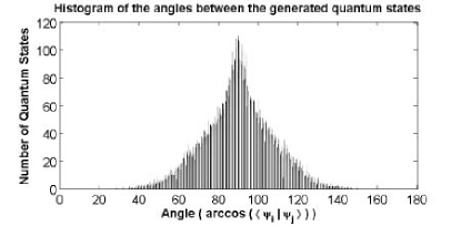
Figure 6: Angles between the generated quantum states for an eight-qubit star graph: Both the Schmidt coefficients and basis are chosen randomly for each state.

When we use the same Schmidt coefficients but different random bases to generate random quantum states; if the sizes of the subsystems are greater than one qubit, the distribution of the histogram of the generated quantum states are still Gaussian. This is numerically shown in Fig.7 for a four-qubit system composed of two-qubit subsystems, $H_{12}$ and $H_{34}$. We draw the distribution of the angles between 1000 random quantum states which has the same Schmidt coefficients but different bases: the comparison of the histograms in Fig.7 and Fig.7 shows that the distributions are very similar when the entanglement between subsystem is high and low. Therefore, if the sizes of the subsystems are greater than one qubit, the amount of the bipartite entanglement between subsystems does not affect the distribution, which is Gaussian.

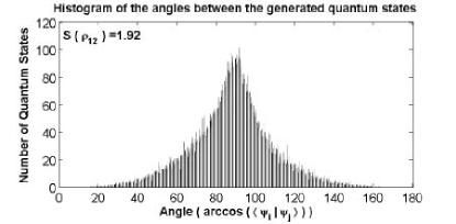
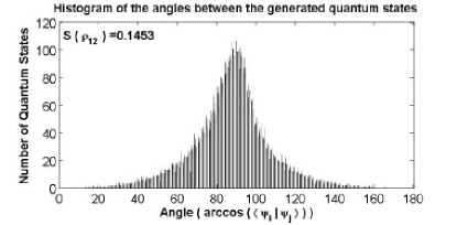
Figure 7: Histograms of the angles between the generated quantum states for four qubits, where the Schmidt coefficients are fixed to certain values and the amount of the entanglement is high in (a) and low in (b).

However, if the size of one of the subsystems is one qubit and the amount of the entanglement is fixed, examples are shown in Fig.8 for an eight-qubit linear graph and in Fig.9 for an eight-qubit star graph, then the distribution of the angles between the generated quantum states are affected by the amount of the bipartite entanglement between these subsystems. As an example in Fig.10 for a two-qubit system, two different random set of Schmidt coefficients are used to generate two group of 1000 quantum random states (the states in the same group have the same Schmidt coefficients): the entanglement is high for the first group and low for the second group. While the histogram of the first group shown in Fig.10 looks more uniform-like, the histogram for the second group shown in Fig.10 is more Gaussian-like. This indicates that the distribution changes by the amount of the entanglement and is Gaussian when the entanglement is low; however, becomes more uniform-like when the amount of the entanglement is increased. This appears more clearly in Fig.11, where the average bipartite entanglement ($\overline{S}$) between subsystems of a five-qubit star graph changes for each different group of 1000 random states. As shown in Fig.11, the distribution becomes more uniform-like when the average entanglement ($\overline{S}$) is increased. Please also note that the reason for using five qubits is to perform the computer simulations faster while keeping the system size large enough. In addition, we show the histograms of star graphs of different number of qubits with different average bipartite entanglements in Fig.12, which also supports Fig.11 and the above argument.

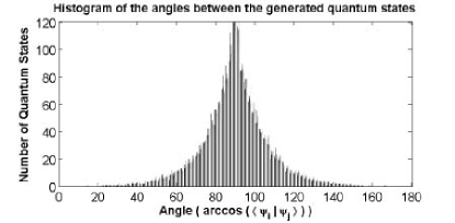
Figure 8: Histogram of the angles between the generated random quantum states for eight qubits where the Schmidt coefficients are fixed and the corresponding bipartite entanglements are given as weights of the edges on the graph.

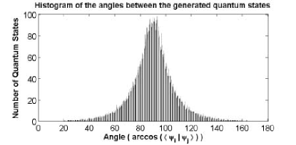
Figure 9: Histogram of the angles between the generated random quantum states for eight qubits where the Schmidt coefficients are fixed and the corresponding bipartite entanglements are given as weights of the edges on the graph.

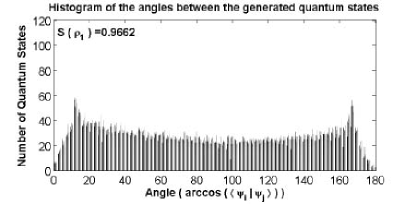
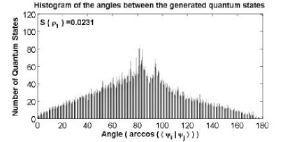
Figure 10: Histograms of the angles between the generated quantum states for two qubits, where the Schmidt coefficients are fixed to a certain value and the amount of the entanglement is high in (a) and low in (b).

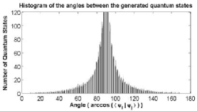
(a) $\overline{S}=0.0838$

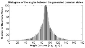
(b) $\overline{S}=0.1974$

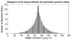
(c) $\overline{S}=0.3012$

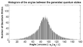
(d) $\overline{S}=0.3887$

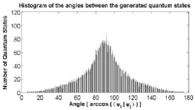
(e) $\overline{S}=0.4735$

(f) $\overline{S}=0.5723$

(g) $\overline{S}=0.6839$

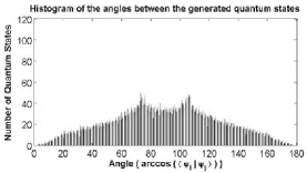
(h) $\overline{S}=0.7655$

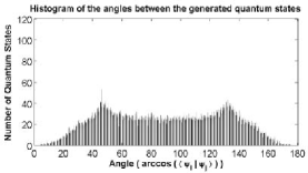
(i) $\overline{S}=0.8578$

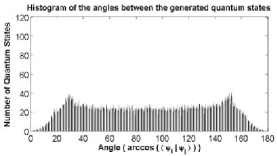
(j) $\overline{S}=0.9440$

Figure 11: Histograms of the angles between the generated quantum states for a 5-qubit star graph, where the Schmidt coefficients are fixed to certain values for each figure and the amount of the average bipartite entanglement ($\overline{S}$) is given under each figure.

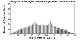
(a) 3-qubit: $\overline{S}=0.5755$

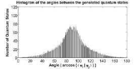
(b) 4-qubit: $\overline{S}=0.2691$

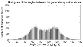
(c) 5-qubit: $\overline{S}=0.6791$

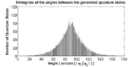
(d) 6-qubit: $\overline{S}=0.4676$

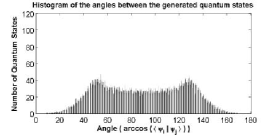
(e) 7-qubit: $\overline{S}=0.8564$

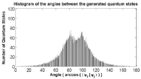
(f) 8-qubit: $\overline{S}=0.6462$

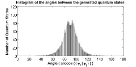
(g) 9-qubit: $\overline{S}=0.5337$

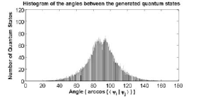
(h) 10-qubit: $\overline{S}=0.6766$

Figure 12: Histograms of the angles between the generated quantum states for different number of qubits, where the Schmidt coefficients are fixed to certain values and the amount of the average bipartite entanglement ($\overline{S}$) is given under each figure.

6 Conclusion

In this paper, we map the Schmidt decomposition for a general quantum state into quantum circuits, which can be used to generate random quantum states. We show that in random state generation, the entanglement amount between subsystems can be controlled by using quantum gates implementing the desired Schmidt coefficients. We also show that one can combine the Schmidt circuits sequentially to generate an equivalent quantum state for an acyclic weighted graph state in which vertices and edges correspond to subsystems and the bipartite entanglement between subsystems, respectively, and also the amount of entanglement is given by the weights of the edges.

Our method can be used in different applications and protocols relying on entanglement. In the simulation of quantum systems, one can use the method to create an instance of the desired system. In addition, decoherence effects the quality of the entanglement and generally cause errors in computations. A similar idea can be used in quantum error correction to correct an imperfect bipartite entanglement, and so a quantum channel.

References

- [1] A. Edelman, N.R. Rao, Acta Numerica 14, 233 (2005). 10.1017/S0962492904000236
- [2] A.M. Tulino, S. Verdú, Random matrix theory and wireless communications, vol. 1 (Now Publishers Inc, 2004)
- [3] C.W.J. Beenakker, Rev. Mod. Phys. 69, 731 (1997). 10.1103/RevModPhys.69.731
- [4] S. Wiesner, SIGACT News 15(1), 78 (1983)
- [5] W.K. Wootters, Foundations of Physics 20(11), 1365 (1990)
- [6] J.J. Sakurai, Modern quantum mechanics (Reading, MA: Addison Wesley,—edited by Tuan, San Fu, 1985)
- [7] H.J. Briegel, R. Raussendorf, Phys. Rev. Lett. 86, 910 (2001). 10.1103/PhysRevLett.86.910
- [8] W. Dür, H. Aschauer, H.J. Briegel, Phys. Rev. Lett. 91, 107903 (2003). 10.1103/PhysRevLett.91.107903
- [9] M. Van den Nest, J. Dehaene, B. De Moor, Phys. Rev. A 69, 022316 (2004). 10.1103/PhysRevA.69.022316
- [10] O. Gühne, G. Tóth, P. Hyllus, H.J. Briegel, Phys. Rev. Lett. 95, 120405 (2005). 10.1103/PhysRevLett.95.120405
- [11] V. Scarani, A. Acin, E. Schenck, M. Aspelmeyer, Phys. Rev. A 71, 042325 (2005). 10.1103/PhysRevA.71.042325
- [12] M. Hein, J. Eisert, H.J. Briegel, Phys. Rev. A 69, 062311 (2004). 10.1103/PhysRevA.69.062311
- [13] D. Schlingemann, R.F. Werner, Phys. Rev. A 65, 012308 (2001). 10.1103/PhysRevA.65.012308
- [14] R. Raussendorf, H.J. Briegel, Phys. Rev. Lett. 86, 5188 (2001). 10.1103/PhysRevLett.86.5188
- [15] M. Hein, W. Dür, J. Eisert, R. Raussendorf, M. Van den Nest, H.J. Briegel, in the Proceedings of the International School of Physics ”Enrico Fermi” on ”Quantum Computers, Algorithms and Chaos”, Varenna, Italy, July 162, 115 (2006). 10.3254/978-1-61499-018-5-115
- [16] C.Y. Lu, X.Q. Zhou, O. Gühne, W.B. Gao, J. Zhang, Z.S. Yuan, A. Goebel, T. Yang, J.W. Pan, Nature Physics 3(2), 91 (2007)
- [17] W. Dür, L. Hartmann, M. Hein, M. Lewenstein, H.J. Briegel, Phys. Rev. Lett. 94, 097203 (2005). 10.1103/PhysRevLett.94.097203
- [18] L. Hartmann, J. Calsamiglia, W. Dür, H.J. Briegel, Journal of Physics B: Atomic, Molecular and Optical Physics 40(9), S1 (2007)
- [19] S. Anders, M.B. Plenio, W. Dür, F. Verstraete, H.J. Briegel, Phys. Rev. Lett. 97, 107206 (2006). 10.1103/PhysRevLett.97.107206
- [20] S. Anders, H.J. Briegel, W. Dür, New Journal of Physics 9(10), 361 (2007)
- [21] E.T. Campbell, J. Fitzsimons, S.C. Benjamin, P. Kok, Phys. Rev. A 75, 042303 (2007). 10.1103/PhysRevA.75.042303
- [22] A.G. White, D.F. James, P.H. Eberhard, P.G. Kwiat, Physical review letters 83(16), 3103 (1999)
- [23] H.J. Briegel, R. Raussendorf, Phys. Rev. Lett. 86, 910 (2001). 10.1103/PhysRevLett.86.910
- [24] M. Sarovar, A. Ishizaki, G.R. Fleming, K.B. Whaley, Nature Physics 6(6), 462 (2010)
- [25] F. Fassioli, A. Olaya-Castro, New Journal of Physics 12(8), 085006 (2010)
- [26] A. Daskin, A. Grama, G. Kollias, S. Kais, The Journal of Chemical Physics 137(23), 234112 (2012). http://dx.doi.org/10.1063/1.4772185
- [27] P. Facchi, U. Marzolino, G. Parisi, S. Pascazio, A. Scardicchio, Phys. Rev. Lett. 101, 050502 (2008). 10.1103/PhysRevLett.101.050502. URL http://link.aps.org/doi/10.1103/PhysRevLett.101.050502
- [28] A. De Pasquale, P. Facchi, G. Parisi, S. Pascazio, A. Scardicchio, Phys. Rev. A 81, 052324 (2010). 10.1103/PhysRevA.81.052324. URL http://link.aps.org/doi/10.1103/PhysRevA.81.052324
- [29] P. Facchi, G. Florio, G. Parisi, S. Pascazio, K. Yuasa, Phys. Rev. A 87, 052324 (2013). 10.1103/PhysRevA.87.052324. URL http://link.aps.org/doi/10.1103/PhysRevA.87.052324
- [30] G. Stewart, SIAM Journal on Numerical Analysis 17(3), 403 (1980)
- [31] T.W. Anderson, I. Olkin, L. Underhill, SIAM Journal on Scientific and Statistical Computing 8(4), 625 (1987)