Existence of Chaos in Plane and its Application in Macroeconomics
Abstract.
The Devaney, Li-Yorke and distributional chaos in plane can occur in the continuous dynamical system generated by Euler equation branching. Euler equation branching is a type of differential inclusion , where are continuous and in every point . Stockman and Raines in [15] defined so-called chaotic set in plane which existence leads to an existence of Devaney, Li-Yorke and distributional chaos. In this paper, we follow up on [15] and we show that chaos in plane with two ”classical” (with non-zero determinant of Jacobi’s matrix) hyperbolic singular points of both branches not lying in the same point in is always admitted. But the chaos existence is caused also by set of solutions of Euler equation branching which have to fulfil conditions following from the definition of so-called chaotic set. So, we research this set of solutions. In the second part we create new overall macroeconomic equilibrium model called IS-LM/QY-ML. The construction of this model follows from the fundamental macroeconomic equilibrium model called IS-LM but we include every important economic phenomena like inflation effect, endogenous money supply, economic cycle etc. in contrast with the original IS-LM model. We research the dynamical behaviour of this new IS-LM/QY-ML model and show when a chaos exists with relevant economic interpretation.
Key words and phrases:
Euler Equation Branching, Chaos, IS-LM/QY-ML Model, Economic Cycle2010 Mathematics Subject Classification:
37N40, 91B50, 91B55Introduction
In this paper we focus on the research of chaos existence in plane . Two dimensional systems are very often in economics, thus the chaos description in plane is very useful and applicable in economics. We follow up on the work of Stockman and Raines in [15]. The core of Devaney, Li-Yorke and distributional chaos existence in plane is based on the special type of differential inclusion called Euler equation branching and on the continuous dynamical system generated by this differential inclusion. The continuous dynamical systems and chaos is also researched in e.g. [17] and the differential inclusions in e.g. [13]. Euler equation branching consists of two branches. The one separate branch is classical two-dimensional system of differential equations. The set of solutions of Euler equation branching contains the solutions only of separate branches and also switching solutions between these two branches. Every branch can produce some singular points and the combination of hyperbolic singular points not lying in the same point of these two branches can provide so-called chaotic set. The definition of chaotic set is provided in [15]. Stockman and Raines in [15] also proved that existence of the chaotic set leads to an existence of Devaney, Li-Yorke and distributional chaos. We provide a comprehensive overview of every possible combinations of hyperbolic singular points of both branches not lying in the same point and we show that so-called chaotic set is there always admitted. We need to have also a set of switching solutions of Euler equation branching which fulfil conditions of the definition of chaotic set, i.e. which are Devaney, Li-Yorke and distributional chaotic, for certainty of the existence of so-called chaotic set in plane , i.e. of Devaney, Li-Yorke and distributional chaos in the dynamical system generated by Euler equation branching in plane . We prove that such chaotic set of solutions exists and that the set of such chaotic sets of solutions are uncountable. We also add some lemmas and remarks to complete the theoretical part of this paper focusing on the existence of chaos in plane .
The economic situation in these days, the phenomena, where the ”classical” (macro-) economic models or the prediction of the future economic progress according these models fail, inspire me to create the new overall macroeconomic model called IS-LM/QY-ML. This new macroeconomic model describes macroeconomic situation including every important economic phenomena like an aggregate macroeconomic equilibrium or (un)stability, an inflation effect, an endogenous money supply, an economic cycle etc. in one overall model. As we can see in this paper, from the perspective of this new model the dynamical behaviour of economy can be very chaotic and unexpected, the aggregate macroeconomic stability can be very frail and sensitive with respect to external influences. New IS-LM/QY-ML model is based on the fundamental macroeconomic IS-LM model. This model explains the aggregate macroeconomic equilibrium, i.e. the goods market equilibrium and the money market or financial assets market equilibrium simultaneously. Already in 1937, J. R. Hicks in [6] published the original IS-LM model as a mathematical expression of J. M. Keynes’s theory. After formulation of the original IS-LM model during many decades many versions of this model and related problems were presented in several works, see e.g. [3], [4], [5], [8], [10], [11] and [19]. The original IS-LM model has several deficiencies, some of subsequent versions deal with modification of this original model but for us requirements we found our way to research this problem and to eliminate the deficiencies of original model. Primarily, Hicks built his model on one concrete economic situation, i.e. the original IS-LM model describes the economy in a recessionary gap. From this follows his assumptions of constant price level and of demand-oriented model. But our overall model describes all phases of the economic cycle and the properties connected with this. So, we firstly include inflation effect to our new model. For do this we inspire by one of the version of original IS-LM model, by IS-ALM model with expectations and the term structure of interest rates, see [2]. Then, we consider also a supply-oriented view of the macroeconomic situation using QY-ML model newly constructed in this paper. The QY-ML model describes simultaneous goods market equilibrium and money market equilibrium under supply-oriented point of view in contrast with IS-LM model. Thus, our new overall IS-LM/QY-ML model consists of two ”sub-models”: demand-oriented ”sub-model” - modified IS-LM and supply-oriented ”sub-model” - new QY-ML model. Depending on the phase of economic cycle the one of these sub-models holds. The switching between these phases is represented by switching between these two sub-models. The mathematical tool to describe the holding of two ”sub-models” and switching between them is exactly Euler equation branching and the continuous dynamical system generated by this differential inclusion. Secondly, Hicks and also economists of that time assumed a strictly exogenous money supply. This supply of money is certain constant money stock determined by central bank. For this conception IS-LM model was the most criticised. The opposite conception is an endogenous money supply which assumes money generated in economy by credit creation, see e.g. [14]. But even today’s economists can not find any consensus in the problem of endogenity or exogenity of money supply, see e.g. [1] or [12]. We resolve this dilemma by conjunction of the endogenous and exogenous conception of money supply including some money supply function to this model.
The dynamical behaviour of new macroeconomic IS-LM/QY-ML model usually leads to hyperbolic singular points of both branches lying in the different point in . So, there possibly exists area of chaotic behaviour of the economy. Furthermore, if some economic cycle with in this article described types or similar types of periods influences economy, then the economy behaves chaotically in the area of given by levels of the aggregate income and of the long-term real interest rate. Besides this also another authors deal with some type of chaos or bifurcations in economics, see e.g. [9] and [18]. In this paper we examine the most typical case of economy describing by IS-LM/QY-ML model and show existence of chaos in such case with relevant economic interpretation of causes. But for less typical cases represented by unusual behaviour of economic subjects this chaos existence possibility is similar.
Summary, this paper consists of two part - the theoretical research about chaos in plane and its application in macroeconomics. In the first theoretical part there is the description of chaos existence in plane which is given by continuous dynamical system generated by special type of differential inclusion called Euler equation branching. In the second application part the new overall macroeconomic equilibrium IS-LM/QY-ML model is constructed and the dynamical behaviour of this model can produce chaos in economy.
1. Preliminaries
All used definitions and theorems in this section follow from [15] and are modified to the special type of differential inclusion in plane .
Definition 1.1.
Let be open set and be continuous. Let us consider differential inclusion given by . We say that there is Euler equation branching in the point if . If there is Euler equation branching in every point than we say that there is Euler equation branching on the set .
Remark 1.1.
The solution of the differential inclusion of Euler equation branching type is function which is the continuous and continuously differentiable a.e. and satisfies . The set of solutions includes the solution of the one branch satisfying , the solution of the second branch satisfying and the ”switching” between these two branches.
In the text below we consider is non-empty open set with Euclidean metric and is time index. Let be set-valued function given by where are continuous and is satisfied for all . , where functions are continuous and continuously differentiable a.e.
Definition 1.2.
The dynamical system generated by is given by
Definition 1.3.
We say that non-empty is compact -invariant set, if is compact and for each there exist a such that and for all .
Let where is compact -invariant set.
Definition 1.4.
Let and is a dynamical system with sense mentioned above. Let , such that . A simple path from to generated by is given by such that , and has finitely many discontinuities on and for all .
Definition 1.5.
Let be a non-empty compact -invariant set and . is so-called chaotic set provided
-
(1)
for all , there exists a simple path from to generated by ,
-
(2)
there exists non-empty and open (relative to ) and such that for all (i.e. there exists such that is not dense in ).
Theorem 1.1.
If is chaotic set then has Devaney chaos.
Theorem 1.2.
If is chaotic set with non-empty interior then has Li-Yorke chaos and distributional chaos.
Theorem 1.3.
If is chaotic set homeomorphic to with and for all , then has Li-Yorke and distributional chaos.
Lemma 1.1.
Let be non-empty closed set such that has unbounded solutions in . Let and let be simple path from to generated by such that (so can be a finite union of arcs and Jordan curves). , ( is number of Jordan curves) denote interiors (bounded components) of such Jordan curves (according to Jordan Curve Theorem). Then is chaotic set.
Theorem 1.4.
Let , and , let be eigenvalues of Jacobi’s matrix of the system in the point and be corresponding eigenvectors. We choose such that for every . Let the solution of be unbounded in (non-empty closed subset of ).
-
(1)
We assume that there exists such that is source (i.e. unstable node or focus) or sink (i.e. stable node or focus) for on . Then admits a chaotic set.
-
(2)
We assume that (i.e. is saddle point) and and , where . Then admits a chaotic set with non-empty interior.
2. Chaos in Continuous Dynamical System
Generated by Euler Equation Branching in plane
First, we show that the existence of so-called chaotic set (see Definition 1.5) is always admitted in the continuous dynamical system generated by Euler equation branching. In some sense, we can find so-called Parrondo’s paradox in this continuous dynamical system. In this way, it means that two asymptotically stable solution of two branches and can produce chaotic sets in the continuous dynamical system generated by Euler equation branching . We extend the theory presented by Stockman and Raines in [15]. We create a comprehensive overview of all possibilities with detecting of so-called chaotic sets (see definition 1.5) in such systems.
The chaotic set has three properties which are connected with the set of solutions . The set contains solutions which are together Devaney, Li-Yorke and distributional chaotic. The element of dynamical system generated by Euler equation branching is solution covering the part corresponding to the branch , the part corresponding to the branch and also information when one branch is switched to the other. We show how such Devaney, Li-Yorke and distributional chaotic set of solutions can look like and we research the set of all Devaney, Li-Yorke and distributional chaotic sets .
We consider only classical singular points corresponding to both branches and , means with non-zero determinant of Jacobi’s matrix of considering system. Furthermore, we consider that the singular points of both branches do not lie in the same point in , means and for . Finally, we assume that both branches produce hyperbolic singular points, i.e. eigenvalues of Jacobi’s matrices corresponding to the branch in the point and to in are not purely imaginary.
The cases where the both branches produce hyperbolic singular points and these points lie in the same point in or at least one branch produce periodic solution (cycle) are not considered in this paper, but the principle and results in these cases seem to be very similar as in the considered case.
2.1. Comprehensive Overview of All Possibilities Admitting Chaotic Set
First we research the possibilities on which Theorem 1.4 can be applicable and which all admit chaotic sets, i.e.
-
•
combinations of sink or source (the stable or unstable node or focus) in the first branch and unbounded solution in in the second branch,
-
•
or combinations of saddle in the first branch and unbounded solution in in the second branch with condition that the trajectory of unbounded solution passing through the saddle point has not the same or the directly opposite direction as the stable or unstable manifold of the saddle point in the point , i.e. the vector is not collinear with the eigenvectors or of the Jacobi’s matrix corresponding to in the point .
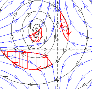
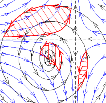
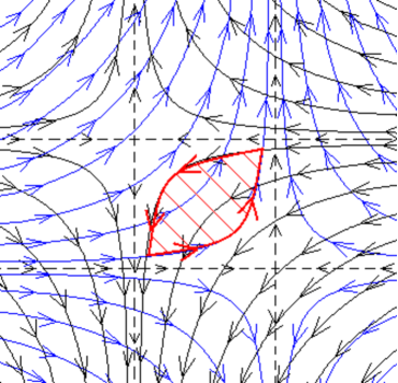
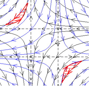
In Table 1 there is the overview of all combinations of hyperbolic singular points, references to the theorems from which the possible existence of chaotic sets and thus Devaney, Li-Yorke and distributional chaos follow, and links to the corresponding figures where the chaotic sets are indicated.
| Branches and | Proof | Fig. |
|---|---|---|
| unstable node - unstable node | Theorem 1.4 (1), 1.1, 1.2 or 1.3 | 4 or 4 |
| unstable node - stable node | Theorem 1.4 (1), 1.1, 1.2 or 1.3 | 4 or 4 |
| unstable node - unstable focus | Theorem 1.4 (1), 1.1, 1.2 | 8 |
| unstable node - stable focus | Theorem 1.4 (1), 1.1, 1.2 | 8 |
| unstable node - unstable saddle | Theorem 1.4 (1) or (2), 1.1, 1.2 or 1.3 | 8 or 8 |
| stable node - stable node | Theorem 1.4 (1), 1.1, 1.2 or 1.3 | 12 or 12 |
| stable node - unstable focus | Theorem 1.4 (1), 1.1, 1.2 | 12 |
| stable node - stable focus | Theorem 1.4 (1), 1.1, 1.2 | 12 |
| stable node - unstable saddle | Theorem 1.4 (1) or (2), 1.1, 1.2 or 1.3 | 17 or 17 |
| unstable focus - unstable focus | Theorem 1.4 (1), 1.1, 1.2 | 17 |
| unstable focus - stable focus | Theorem 1.4 (1), 1.1, 1.2 | 17 |
| unstable focus - unstable saddle | Theorem 1.4 (1) or (2), 1.1, 1.2 | 20 |
| stable focus - stable focus | Theorem 1.4 (1), 1.1, 1.2 | 17 |
| stable focus - unstable saddle | Theorem 1.4 (1) or (2), 1.1, 1.2 | 20 |
| unstable saddle - unstable saddle | Theorem 1.4 (2), 1.1, 1.2 | 20 |
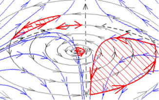
On the illustrative figures we present the both situations, where the branch corresponds to the black trajectories or to the blue trajectories according to relevant theorems. That is why there are predominately two figured chaotic sets. The chaotic sets are displayed by red hatched areas. The arrows show the directions of the trajectories. The principle of such chaotic behaviour is based on switching between these two branches. First the solution of such system goes alongside the black trajectory in direction of the corresponding arrow, then this solution switches to the second branch and goes alongside the blue trajectory in direction of the corresponding arrow etc. And vice versa, the moving point can go first alongside the blue trajectory and then after system switch alongside the black trajectory etc.
![[Uncaptioned image]](/html/1403.0111/assets/x1.png)
![[Uncaptioned image]](/html/1403.0111/assets/x2.png)
![[Uncaptioned image]](/html/1403.0111/assets/x3.png)
![[Uncaptioned image]](/html/1403.0111/assets/x4.png)
![[Uncaptioned image]](/html/1403.0111/assets/x5.png)
![[Uncaptioned image]](/html/1403.0111/assets/x6.png)
![[Uncaptioned image]](/html/1403.0111/assets/x7.png)
![[Uncaptioned image]](/html/1403.0111/assets/x8.png)
![[Uncaptioned image]](/html/1403.0111/assets/x9.png)
![[Uncaptioned image]](/html/1403.0111/assets/x10.png)
![[Uncaptioned image]](/html/1403.0111/assets/x11.png)
![[Uncaptioned image]](/html/1403.0111/assets/x12.png)
![[Uncaptioned image]](/html/1403.0111/assets/x13.png)
![[Uncaptioned image]](/html/1403.0111/assets/x14.png)
![[Uncaptioned image]](/html/1403.0111/assets/x15.png)
![[Uncaptioned image]](/html/1403.0111/assets/x16.png)
![[Uncaptioned image]](/html/1403.0111/assets/x17.png)
Now, we research the possibilities which are not considered above and on which Theorem 1.4 can not be applicable. These possibilities are cases when the trajectory of unbounded solution passing through the saddle point has the same or the directly opposite direction as the stable or unstable manifold of the saddle in the point , means the vector is collinear with the eigenvectors or . We show that every such possibilities can produce chaotic sets.
Let remind notations: , and , are eigenvalues of Jacobi’s matrix of the system in the point and are corresponding eigenvectors. We choose such that the solution of is unbounded in and for every .
Theorem 2.1.
Let (i.e. is saddle point) and or , where . Then admits a chaotic set.
Proof.
Let denote flow generated by and denote flow generated by . Let denote stable manifold and denote unstable manifold corresponding to . Because and are continuous, the solution corresponding to in is unbounded and for every , then for sufficiently small we can distinguish two possible cases:
-
(1)
for every or for any ;
-
(2)
for every or for some .
can not be zero. Zero would lead to , but we assume the opposite ( for every ).
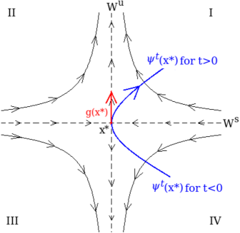
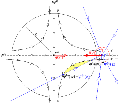
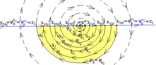
Ad (1) Assume is unstable saddle point, or where , and for every or for any . The stable manifold and the unstable manifold corresponding to divide the ball in four quadrants (I, II, III, IV). We consider (corresponding to ). The condition and for every for any imply that for sufficiently small neighbourhood of the point the flow is in the quadrant for (or ) sufficiently close to and in the quadrant mod for (or ) sufficiently close to for some , see the Figure 21. It depends on notations of quadrants and on positions of and .
Without loss of generality we consider that for is in the quadrant IV and for is in the quadrant I, see Figure 21. Thus, let be maximal and be minimal such that , see Figure 22. Then let and be maximal and be minimal () such that and , see Figure 22.
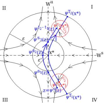
Thus, there exists such that for all and such that , and for some , see the Figure 22. So now, we are interested only in quadrant III. If we have the opposite direction of , then we will be interested in the quadrant II, see the Figure 22. Then, firstly we choose such that , see Figure 23. Secondly, we choose such that if then for every , see Figure 23. At the end we pick . So, and thus for all . Hence there exists such that , see Figure 23.
Hence there exist a simple path from to which consists of two arcs and , where , and . Then according Lemma 1.1 admits chaotic set (i.e. yellow area on Figure 23). Like this constructed chaotic set has obviously non-empty interior (has non-empty bounded component, see Lemma 1.1). The proof for is analogous.
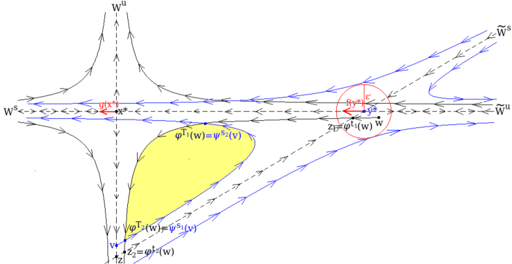
Ad (2) Assume is unstable saddle point, or , where , and for every or for some ( can be different for each ). We consider (corresponding to ). The condition and for every for some imply that overlaps in , see Figure 24.
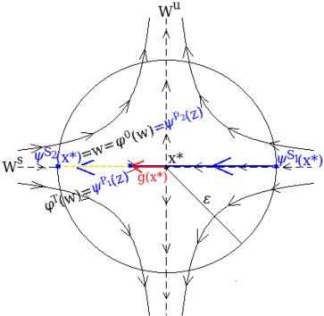
Thus, let be maximal and be minimal such that , see Figure 24. Let . Thus there exist such that , see Figure 24. Hence there exist a simple path from to which consists of two arcs and , where , and . Then according Lemma 1.1 admits chaotic set (i.e. yellow line segment on Figure 24). Like this constructed chaotic set is obviously homeomorphic to with and for all . The proof for is analogous with reverse time direction and with . ∎
Remark 2.1.
Even though we construct only a chaotic set homeomorphic to with and for all in the part (2) of the proof of Theorem 2.1, there can exist also a chaotic sets with non-empty interior in the cases describing below. Let further , , eigenvalues of the Jacobi’s matrix of in the with corresponding eigenvectors .
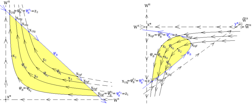
For node type of the second singular point the chaotic set with non-empty interior exists if overlaps the whole or since the point . We show this for . Hence and , see Figure 25.
Then we choose . Thus for sufficiently large (means sufficiently large ) there exist for some , and for some , such that and , see Figure 25. Hence admits the chaotic set (i.e. yellow area in Figure 25) consisting of two arcs and , where and , and its (non-empty) interior. The construction for is analogous.
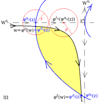
For saddle type of the second singular point the chaotic set with non-empty interior exists if stable manifold corresponding to the saddle overlaps the whole unstable manifold corresponding to the saddle since the point and the unstable manifold corresponding to intersects the stable manifold corresponding to . And vice versa. We consider the first possibility. The construction for the second possibility is analogous. Hence and . Let the intersection of and denote , see Figure 26. Let denote the ”triangle” given by the points , and .
Then we choose . Thus for sufficiently large there exist such that there exist and for some and some , see Figure 26. Then there certainly exists for some (corresponding to ) such that for some and for some , see Figure 26. Thus admits the chaotic set (i.e. yellow area on Figure 26) consisting of two arcs and , where and , and its (non-empty) interior.
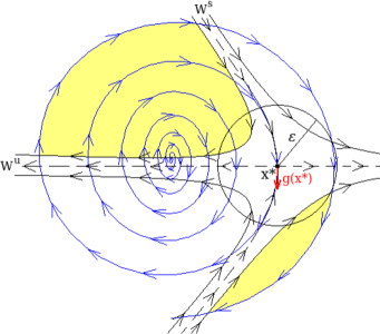
If type of the second singular point is focus, then there always exists chaotic set with non-empty interior. The focus type of singular point naturally ensures such chaotic set, see yellow area on Figure 27.
The existence of chaotic set with non-empty interior in the case describing by the part (2) of the proof of Theorem 2.1 is provided by appropriate trajectory corresponding to which has to intersect first in time and then in non-degenerated case (see Figure 23) or which has to intersect the separate not overlapped manifold in two points in degenerated case (see Figure 26).
In the Table 2 we illustrate all remaining combinations of hyperbolic singular points where or . There are references to the part of the proof of previous Theorem 2.1 which proves the possible existence of chaotic sets, and thus Devaney, Li-Yorke and distributional chaos according to relevant theorems, and links to the corresponding figures where the chaotic sets are indicated. There is also description how the mutual positions of these pairs of hyperbolic singular points are on next illustrative Figures 31-42.
| Branches and | Proof | Fig. |
| unstable saddle - unstable node: | ||
| - node lies outside manifolds | Theorem 2.1 (1), 1.1, 1.2 | 31 |
| - node lies on unstable manifold | Remark 2.1, Theorem 2.1 (2), 1.1, 1.2, 1.3 | 31 |
| - node lies on stable manifold | Theorem 2.1 (2), 1.1, 1.3 | 35 |
| unstable saddle - stable node: | ||
| - node lies outside manifolds | Theorem 2.1 (1), 1.1, 1.2 | 31 |
| - node lies on stable manifold | Remark 2.1, Theorem 2.1 (2), 1.1, 1.2, 1.3 | 31 |
| - node lies on unstable manifold | Theorem 2.1 (2), 1.1, 1.3 | 35 |
| unstable saddle - unstable focus | Theorem 2.1 (1), 1.1, 1.2 | 35 |
| Remark 2.1, Theorem 2.1 (2), 1.1, 1.2, 1.3 | 38 | |
| unstable saddle - stable focus | Theorem 2.1 (1), 1.1, 1.2 | 35 |
| Remark 2.1, Theorem 2.1 (2), 1.1, 1.2, 1.3 | 38 | |
| unstable saddle - unstable saddle: | ||
| - manifolds are not overlapped | Theorem 2.1 (1), 1.1, 1.2 | 38 |
| - stable manifold overlaps | Remark 2.1, Theorem 2.1 (2), 1.1, 1.2, 1.3 | 42 |
| unstable manifold and second | ||
| manifolds intersect each other | ||
| - stable manifold overlaps | Theorem 2.1 (2), 1.1, 1.3 | 42 |
| unstable manifold and second | ||
| manifolds do not intersect | ||
| - stable manifolds are overlapped | Theorem 2.1 (2), 1.1, 1.3 | 42 |
| - unstable manifolds are overlapped | Theorem 2.1 (2), 1.1, 1.3 | 42 |
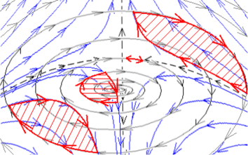
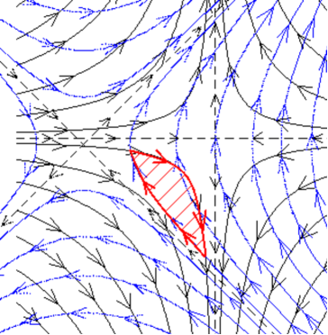
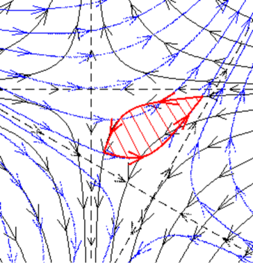
On the illustrative figures we present the both situations, where the branch corresponds to the black trajectories or to the blue trajectories according to relevant theorems, similarly as above. For application of Theorem 2.1 we must consider the blue trajectories belong to the first branch , where the type of hyperbolic singular point is unstable saddle, then the black trajectories belong to the second branch , where the type of hyperbolic singular point is various. The chaotic sets are figured by red hatched areas. In the red hatched area (chaotic set) we go first along the black trajectories in direction indicated by corresponding arrows, then we switch on the blue trajectories and go along these trajectories in direction indicated by corresponding arrows etc., or vice versa.
![[Uncaptioned image]](/html/1403.0111/assets/x29.png)
![[Uncaptioned image]](/html/1403.0111/assets/x30.png)
![[Uncaptioned image]](/html/1403.0111/assets/x31.png)
![[Uncaptioned image]](/html/1403.0111/assets/x32.png)
![[Uncaptioned image]](/html/1403.0111/assets/x33.png)
![[Uncaptioned image]](/html/1403.0111/assets/x34.png)
![[Uncaptioned image]](/html/1403.0111/assets/x35.png)
![[Uncaptioned image]](/html/1403.0111/assets/x36.png)
![[Uncaptioned image]](/html/1403.0111/assets/x41.png)
![[Uncaptioned image]](/html/1403.0111/assets/x42.png)
![[Uncaptioned image]](/html/1403.0111/assets/x43.png)
![[Uncaptioned image]](/html/1403.0111/assets/x44.png)
2.2. Devaney, Li-Yorke and Distributional Chaotic Set of Solutions
In the previous section 2.1, we show that the chaotic set is always admitted in with two hyperbolic singular points not lying in the same point but the existence of chaos also depends on set of solutions generating solutions ensuring the chaotic set , see Definition 1.5.
Let us remind: the dynamical system generated by Euler equation branching , , continuous and continuously differentiable a.e., non-empty, compact -invariant set and . The solution from is composed of the part corresponding to the solution of the branch , of the part corresponding to the solution of the branch and of the switching system between these two branches. For each point the solution contains also the consequence of times such that and for odd give the times of switching from the branch to and for even give the times of switching from the branch to , if we start by branch , or vice versa (odd for switch from to and even for switch from to ), if we start by branch . From the nature of such solutions follows that for each point there exist uncountable many solutions differing just in such switching system.
The set of solutions corresponding to has to fulfil three conditions to be Devaney, Li-Yorke and distributional chaotic - every solution ”stays forever in ” (F-invariant set and definition of ), each point ”can be connected with each another point” in by simple path given by some (the property (1) of chaotic set ) and there exists such that is not dense in (the property (2) of chaotic set ).
Theorem 2.2.
In dynamical system generated by Euler equation branching in there exists the set of solutions which ensures chaotic set , hence this set is Devaney, Li-Yorke and distributional chaotic. Moreover the set of such is uncountable.
Proof.
We assume that starting point is influenced firstly by branch , i.e. the consequence of switching times is such that and for odd give the times of switching from the branch to and for even give the times of switching from the branch to . So, we consider , , , such that the solution of is unbounded in and for every . If we assume an opposite situation (start in ), then the proof will be analogous with difference that we consider and unbounded solution of in etc. Denote by and the flow belonging to and to .
First, we construct such set of solutions for with non-empty interior. We initially assume is unstable (node, focus, saddle). We denote by a chaotic set of solutions . We describe the solutions using the Figure 43 for node, using the Figure 44 for focus, and using the Figure 45 for saddle. By yellow areas the sets are figured. If is node, the set is bounded by trajectory of denoted by arbitrary closed to the trajectory of (figured by dashed line) passing through the point and by arbitrary trajectory of denoted by intersecting trajectory in two points such that for some , it holds and and for every , see Figure 43.
If is focus, the set is bounded by trajectory of denoted by passing through the point and by arbitrary trajectory of denoted by intersecting trajectory in two points such that for some , it holds and and for every and for every , see Figure 44.
If is saddle, the set is bounded by arbitrary trajectory of denoted by intersecting the unstable manifold in time and the stable manifold in time such that and by arbitrary trajectory of denoted by intersecting trajectory in two points such that for some , it holds and and for every , see Figure 45 (on the left), in ”non-degenerated” case describing by Theorem 1.4 (2) or by part (1) of the proof of Theorem 2.1. In ”degenerated” case describing by Remark 2.1, where stable manifold of one saddle overlaps the unstable manifold of the second saddle, the set is bounded by arbitrary trajectory of denoted by intersecting the separate not overlapped manifold in two points and by arbitrary trajectory of denoted by intersecting trajectory in two points. Let and for some , , see Figure 45 (on the right).
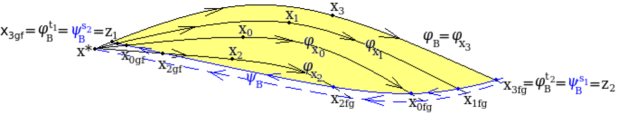
For every point the solution is given by the trajectory of branch denoted by from the point to the point , then by the trajectory from the point to the point , then by the trajectory from the point to the point through the point and so on, see Figure 43 for node , see Figure 44 for focus and see Figure 45 for saddle . So, the solution is given by consequence of time , , , , , such that , , , . We denote by the solutions which are described below. For every point the solution passing through every point () is given by the trajectory of branch (denoted by ) from the point to the point , then by the trajectory from the point to the point , then by the trajectory of denoted by passing through the point from the point to the point , then by the trajectory from the point to the point , then by the trajectory from the point through the point to the point , then by the trajectory from the point to the point etc., see e.g. for the point on Figure 43 for node , on Figure 44 for focus and on Figure 45 for saddle . So, the solution is given by the consequence of the time , , , , and , such that , , , , , . Especially for starting points lying on (we start with the switch). It is obvious that fulfils three conditions mentioned above to be chaotic. The solutions and also every ”stay forever in ”. Each point ”can be connected with each another point” in by some or . Neither nor for every are dense in . The proof for stable node or stable focus is analogous with reversed time direction.
The construction of set of solutions for homeomorphic to is similar. The set is the curve segment with two distinct end points not containing or where for all , i.e. where the trajectories corresponding to the flows and have the opposite direction, see Figure 4, 4, 8, 12, 17, 31-35, 38, 38 or 42-42. Let and be trajectories corresponding to and such that and for some , where and be two distinct end points of the curve segment, see Figure 46.
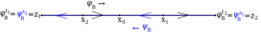
Let analogously be a chaotic set of solutions . We describe the solutions using Figure 46. The chaotic set is displayed by curve with two distinct end points and , see Figure 46. For every point the solution is given by the trajectory from the point to the point , then by the trajectory from the point to the point , then by the trajectory from the point to the point and so on, see Figure 46. So, the solution is given by consequence of time , , , such that , , . We denote analogously by the solutions which are described below. For every point the solution denoted per , () is given by the trajectory from the point to the point , then by the trajectory from the point to the point , then by the trajectory from the point to the point , then by the trajectory from the point to the point etc., see e.g. for the point on Figure 46. So, the solution is given by the consequence of the time , , , and , such that , , , , . Especially for starting points (we start with the switch). It is analogously obvious that is chaotic chaotic set of solutions.
At the end of the proof, we remark that from the nature of such type of set of solutions follows uncountability of the set of such . We can construct uncountable many sets of solutions based on presented construction. Let be set of solution such that for every the moving point goes on the trajectory of from the point to the point or , then on the trajectory of from the point or to the point where or to where , then on the trajectory of to the point or , then on the trajectory of to the point where or to where , then on the trajectory of to the point or , then on the trajectory of to the point or , then on the trajectory of to the point or etc., see Figure 43, 44, 45 or 46. Let similarly be set of solution such that for every the moving point goes on the trajectory of from the point to the point or , then on the trajectory of from the point or to the point where or to where , then on the trajectory of to the point or , then on the trajectory of again to the point where or to where , then on the trajectory of to the point or , then on the trajectory of to the point or , then on the trajectory of to the point or etc., see Figure 43, 44, 45 or 46. Then or is chaotic set of solutions. We can construct in this way uncountable many sets of solutions based on combinations of every relevant path (”loops” and number of the same ”loops”) of solutions .
∎
Remark 2.2.
In the proof of Theorem 2.2 there are described boundaries of chaotic set with non-empty interior but every combination of considered singular points has a ”maximal” area in plane where the chaotic sets can exist as we can discern on Figures 4-20 and 31-42. For example the combination of two unstable nodes has this area bounded by trajectory of passing through the point and by the trajectory of passing through the point (without these trajectories), see Figure 4. For another example in the case of unstable and stable node this area is consists of two disconnected parts. The first part is bounded by trajectory of passing through the point and by the last trajectory of intersected this trajectory of (without this trajectory corresponding to ), and vice versa the second part is bounded by the trajectory of passing through the point and by the last trajectory of intersected this trajectory of (without this trajectory corresponding to ), see Figure 4. In the combination of two foci this maximal area is bounded analogously by first trajectories passing through the point or (with these trajectories) and this area can be one connected part or can consist of two disconnected parts and can not contain or as an interior point, i.e. or lies on the boundary line, see Figure 17, 17 or 17. From Remark 2.1 for ”degenerated” case of combination of two saddles (stable manifold of one saddle overlaps the unstable manifold of the second saddle) follows that this maximal area is bounded by ”triangle” (without boundary manifolds), see Figure 26. In fact in this special case there are another areas where chaotic sets can exist. These areas are situated in ”half-plane” bounded by the overlapped manifold and containing , but the concrete position of this area depends of concrete situation.
Lemma 2.1.
The Devaney, Li-Yorke and distributional chaotic can not be set of only one solution .
Proof.
If the set contains only one solution then such solution will not fulfil both property (1) and (2) from Definition 1.5 together. Obviously, we can use only one solution to ensure property (1) (we want to every pair be scrambled), hence has to go through every point of the set . But then is dense in . But either such solution is not Devaney, Li-Yorke and distributional chaotic itself because the points lying in the same trajectory (corresponding or ) are not scrambled. ∎
Lemma 2.2.
The set of all Devaney, Li-Yorke and distributional chaotic sets of solutions on is not dense or nowhere dense in ( restricted on ).
Proof.
Consider restricted on . Let be the power set of (the set of all subset of ), be set of all Devaney, Li-Yorke and distributional chaotic sets of solutions and be set of all non-chaotic sets of solutions . Obviously and . , see Theorem 2.2, and , non-chaotic set of solutions is for example the set of only one , see Lemma 2.1, or of not F-invariant . We have topological space with discrete topology. . So, , hence is not dense in . Similarly and , hence is not nowhere dense in . ∎
Remark 2.3.
It is obvious that in dynamical system there exist solutions corresponding only to the one branch without branch switching, or solutions ”running out” the set . The ”force” causing the switch is exogenously determined. It is required the switch before solution leaves the set . And there has to be the reason depending on concrete modelled problem for this switch. It also depends on interpretation, see the application part of this paper - section 3.
3. Application in Macroeconomics
In this section we apply the theoretical findings from previous section in macroeconomics. We construct the new overall macroeconomic equilibrium model containing two branches - demand-oriented and supply-oriented and for connection of these two branches we use Euler equation branching. The switching between these two branches is interpreted by influence of the economic cycle. Then we describe economic behaviour of such overall model leading to the chaos and we submit reasonable economic interpretation of a cause of such behaviour.
3.1. Construction of New Overall Macroeconomic Equilibrium Model
This new macroeconomic equilibrium model describes the macroeconomic situation in two sector economy, precisely the goods market equilibrium and the money market equilibrium simultaneously including every important economic phenomena like an economic cycle, an inflation effect, an endogenous money supply etc. in one overall model. This model follows from fundamental macroeconomic equilibrium model called IS-LM model. The original IS-LM model is strictly demand-oriented, assumes a constant price level and an exogenous money supply. This original conception is obsolete. Thus, we create new model eliminating these deficiencies and containing also a supply-oriented part. The demand-oriented model (the modified IS-LM model) holds in the recession and the supply-oriented model (the new QY-ML model) holds in the expansion. Then we join these two (sub-)models to one overall model called IS-LM/QY-ML by Euler equation branching interpreted by existence of economic cycle. So, we first present the modified IS-LM model eliminating mentioned deficiencies of the original model, then we construct the new QY-ML model supply oriented, then we explain when these models hold and at the end we join these two ”sub-models” two one overall IS-LM/QY-ML model.
3.1.1. Demand-Oriented Sub-model - Modified IS-LM Model
We can find the original IS-LM model in e.g. [5]. This model describes aggregate macroeconomic equilibrium, i.e. the goods market equilibrium and the money market (or financial assets market) equilibrium simultaneously from the demand-oriented point of view. The demand-oriented model means that the supply is fully adapted to the demand. Here, we present our modification of the original model which eliminates its deficiencies or obsolete assumptions. This model is still demand-oriented but we eliminate the assumption of constant price level by modelling of inflation and the assumption of strictly exogenous money supply by connection of the endogenous and exogenous conception of the money supply.
Definition 3.1.
The modified IS-LM model is given by the following system
| (1) |
where
is time,
is aggregate income (GDP, GNP),
is long-term real interest rate,
is investment function,
is saving function,
is money demand function,
is money supply function,
is money stock determined by central bank,
is maturity premium,
is expected inflation rate,
are parameters of dynamics.
Remark 3.1.
The goods market from the demand-oriented point of view is described by equation IS. Analogously the money market from the demand-oriented point of view is described by the equation LM. There are the investment and saving function on the goods market and the money demand function and money supply function on the money market. We suppose that all of these functions are differentiable.
Remark 3.2.
The main variables in the original IS-LM model is the aggregate income and the interest rate . In the modified model, we eliminate the original assumption of constant price level, so we need to distinguish two type of interest rate - a long-term real interest rate and a short-term nominal interest rate . There is the long-term real interest rate on the goods market and the short-term nominal interest rate on the money market (or financial assets market). The well-known relation holds. The sort-term nominal interest rate is positive and long-term real interest rate can be also negative because of an inflation rate. While and are constants, holds.
Remark 3.3.
The one of the main criticised assumption of the original IS-LM model is an assumption of strictly exogenous money supply. This means that the money supply is some money stock determined by central bank. The endogenous money supply means that money is generated in economy by credit creation. Today’s economists can not find any consensus between these two conceptions of the money supply. So, we join these two conceptions into one. We consider that the money supply is the endogenous quantity (some new defined function ) with some exogenous part (constant ).
Remark 3.4.
The curve IS represents the goods market equilibrium. The curve IS is the set of ordered pairs fulfilling . Similarly, the curve LM represents the money market equilibrium. The curve LM is the set of ordered pairs fulfilling . So, the aggregate macroeconomic equilibrium (i.e. equilibrium on goods market and on money market, or on financial assets market, simultaneously) is the intersection point (one or more) of the curve IS and the curve LM. In the dynamic version we research the (un)stability of this macroeconomic system.
Definition 3.2.
Economic properties of the functions , , and are the following:
| (2) |
| (3) |
| (4) |
| (5) |
Remark 3.5.
The economic properties of the investment, saving and money demand function are standard. The economic properties of the new defined money supply function means that the relation between supply of money and aggregate income and also interest rate is positive and that the rate of increase of money supply depending on aggregate income is smaller than the rate of increase of money demand depending on aggregate income because the banks are more cautious than another subjects. and hold, because we assume constant and .
3.1.2. Supply-Oriented Sub-model - New QY-ML Model
In this subsection we construct new model describing the aggregate macroeconomic equilibrium or (un)stability which is supply-oriented in opposite of the IS-LM model. The construction of this new model is similar as of the IS-LM model. We find the simultaneous equilibrium on the goods market and on the money market but under assumption that the demand is fully adapted to the supply. We also consider the floating price level and the endogenous money supply with some exogenous part in the same way as in the modified IS-LM model.
Definition 3.3.
The QY-ML model is given by the following system
| (6) |
where
is time,
is aggregate income (GDP, GNP),
is long-term real interest rate,
is production function,
is capital function,
is labour function,
is technical progress function,
is money supply function,
is money stock determined by central bank,
is money demand function,
is maturity premium,
is expected inflation rate,
are parameters of dynamics.
Remark 3.6.
Thus, how do we proceed during the construction? If the goods demand is fully adapted to the goods supply, than the aggregate production has to be covered by demand. So, the supply side is represented by some aggregate production function and the demand side is represented by level of aggregate income on the goods market. The production is the function of capital , labour and technical progress . We will consider that , and are dependent on aggregate income and long-term real interest rate . Summary, . So, the goods market from the supply-oriented point of view is described by equation QY. The money demand is fully adapted to the money supply, so we have the equation ML to describe the money market from the supply-oriented point of view. There are the production function on the goods market and the money supply and money demand function on the money market. We suppose that all of these functions are differentiable.
Remark 3.7.
The curve QY represents the goods market equilibrium. The curve QY is the set of ordered pairs fulfilling . Similarly, the curve ML represents the money market equilibrium. The curve ML is the set of ordered pairs fulfilling . So, the aggregate macroeconomic equilibrium (i.e. the equilibrium on goods market and on money market, or on financial assets market, simultaneously) is the intersection point (one or more) of the curve QY and the curve ML. In the dynamic version we research the (un)stability of this macroeconomic system.
Definition 3.4.
Economic properties of the aggregate production function are given by
| (7) |
Economic properties of the production factors functions are the following
| (8) |
| (9) |
Remark 3.8.
The economic interpretation of these properties is following. If the production factors (i.e. capital, labour and technical progress) are increased then the aggregate production will increase. The relations between production factors (, , ) and aggregate income () are positive. And the relations between production factors (, , ) and long-term real interest rate () are negative.
3.1.3. Influence of Economic Cycle
The previous ”sub-models” hold in the different economic situations. This holding of demand-oriented and supply-oriented ”sub-model” and switching between them depends on the phase of the economic cycle. In this section, we explain this context. On the Figure 47, there is illustrated the economic cycle. We can see its phases: expansion, peak, recession, trough and so on along the economic growth trend.
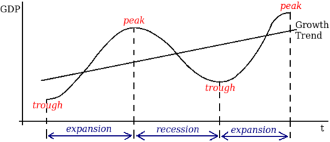
The demand-oriented ”sub-model” - modified IS-LM model holds in the recession phase. In the recession the economy is under the production-possibility frontier. So, the firms can flexibly react on the demand, thus the supply is adapted to the demand. In the trough the economic situation is changed. The demand-oriented ”sub-model” is switched to the supply-oriented ”sub-model”. Then, there is the expansion phase where supply-oriented model - new QY-ML model holds. In the expansion the production increases, the production factors are sufficiently rewarded and change theirs income to the aggregate demand. So, the demand is adapted to the supply (aggregate production). The new QY-ML model holds until the peak where the economic situation is changed. In the peak the supply-oriented ”sub-model” is switched to the demand-oriented ”sub-model”. Further, the cycle continues in such a way. We summarize this mechanism in Table 3.
| Phase | Orientation | Describing by |
|---|---|---|
| Recession | Demand-oriented model | Modified IS-LM model |
| Trough | Changing from demand-oriented | Switching from IS-LM model |
| to supply-oriented model | to QY-ML model | |
| Expansion | Supply-oriented model | New QY-ML model |
| Peak | Changing from supply-oriented | Switching from QY-ML model |
| to demand-oriented model | to IS-LM model |
3.1.4. Overall Macroeconomic IS-LM/QY-ML Model
In this subsection, we formulate the overall macroeconomic IS-LM/QY-ML model. This model consists of demand-oriented ”sub-model” - the modified IS-LM model (defined in subsection 3.1.1) and of supply-oriented ”sub-model” - the new QY-ML model (defined in subsection 3.1.2). These two ”sub-models” are connected by Euler equation branching (see Definition 1.1).
Definition 3.5.
The overall macroeconomic IS-LM/QY-ML model is given by the following differential inclusion
| (10) |
where , constant and parameters of dynamics , , , .
The investment function , saving function , money demand function , money supply function and aggregate production function have the previously introduced economic properties (2), (3), (4), (5) and (7). The production factors functions have the economic properties (8) and (9) mentioned above.
The solutions of this differential inclusion are solutions of demand-oriented branch (IS-LM model), of supply-oriented branch (QY-ML model) and also switching between these two branches. These solutions follow from the economic cycle, see the previous subsection 3.1.3.
This presented differential inclusion with two branches generates a continuous dynamical system describing overall macroeconomic situation in every phase of economic cycle.
3.2. Chaos in IS-LM/QY-ML Model
In this section, we describe a dynamical behaviour of the system (10) with relevant economic interpretation. In economics, equilibrium points are important. The equilibrium point represents an ideal situation where the demand is equal to the supply. In our situation the equilibrium points on the goods market are points of whole curve IS or QY and the equilibrium points on the money market are points of whole curve LM=ML. So, the overall macroeconomic equilibrium (simultaneous equilibrium on goods and money market) is represented by intersection point(s) of the curve IS and LM, or QY and ML. But the economic situation relevant to the equilibrium is very rare. Thus, the description of disequilibrium points are more important. Such disequilibrium points are all other points in plane given by . There commonly exists an excess of goods demand, an excess of goods supply, or an excess of money demand and an excess of money supply. A description of dynamical behaviour of our IS-LM/QY-ML model using phase portraits show us behaviour of the moving point in the area of disequilibrium points more than in equilibrium points.
We show the dynamical behaviour of the most typical economic case of IS-LM/QY-ML model. We consider the modified IS-LM model described by (1) with economic functions properties (2), (3), (4), (5). The typical IS curve is decreasing and the typical LM curve is increasing. Using Implicit Function Theorem we see that properties (4) and (5) ensure increasing LM curve. If we furthermore assume
| (11) |
in addition to the properties (4) and (5) then the curve IS is decreasing. We know that and . Now, let denote a function whose graph is the curve IS, and denote the function whose graph is the curve LM. These functions exist because of Implicit Function Theorem. If we assume
| (12) |
in addition to the conditions (2), (3), (4), (5) and (11) then there exists one intersection point of the curve IS and LM.
Proposition 3.1.
Proof.
The eigenvalues of Jacobi’s matrix of the system (1) in this singular point are
where . The real part of eigenvalues in this point because of (11), according to (4) and (5) and according to economic condition (2), (3), (4), (5) and (11). From this follows that this singular point is stable node if in addition or stable focus if in addition .
∎
Now, we consider new QY-ML model described by (6) with economic functions properties (4), (5), (7), (8) and (9). Using Implicit Function Theorem we see that properties (4) and (5) ensure increasing ML curve. If we furthermore assume
| (13) |
in addition to the properties (7), (8) and (9) like analogy to the condition and on the goods market then the curve QY is decreasing. Analogously let denote a function whose graph is the curve QY, and denote the function whose graph is the curve ML. These functions exist because of Implicit Function Theorem. If we assume
| (14) |
in addition to the conditions (4), (5), (7), (8), (9) and (13) then there exists one intersection point of the curve QY and ML.
Proposition 3.2.
Proof.
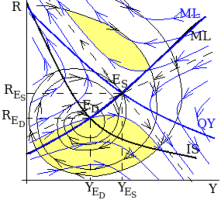
We can see curve IS and LM and stable focus as equilibrium point of IS-LM model displayed on Figure 49. The curve QY and ML and unstable saddle as equilibrium point of QY-ML model are shown on Figure 49.
![[Uncaptioned image]](/html/1403.0111/assets/x50.png)
![[Uncaptioned image]](/html/1403.0111/assets/x51.png)
Now, if we consider the differential inclusion (10) consisting of the IS-LM model (1) and of the QY-ML model (6) with economic functions properties (2), (3), (4), (5), (7), (8), (9), (11), (12), (13) and (14), then there chaotic sets in plane (with variables ) are admitted, see yellow areas on Figure 50.
As we present in the section 2.2 we need to have Devaney, Li-Yorke and distributional chaotic set of solutions for chaos existence in plane . We use the set of solutions from the proof of Theorem 2.2. It is necessary to provide some economic interpretation or economic explanation of such set of solutions .
-
•
The solution describes an economy in the regular economic cycle where the expansion phase has still the same duration and also the recession phase. Thus, this economic cycle has still the same period. In plane describing by ordered pairs the concrete changes of aggregate income and interest rate during the expansion and recession phase are the same in every period.
-
•
The solutions describes more irregular economic cycle. The period of whole (one) cycle is different in two consecutive periods. Every solution explains every relevant change in the following period duration.
For node or focus types of equilibrium points of the IS-LM and QY-ML model the trajectory corresponding to the IS-LM model passing through the equilibrium of the QY-ML model and the trajectory corresponding to the QY-ML model passing through the equilibrium of the IS-LM model is critical and very ”strong”. It is critical trajectory because we have to overcome the frontier given by this trajectory to get out of the chaotic area. It is ”strong” trajectory because the market economy ”inclines” to the equilibrium points, which are ideal states, and this trajectory ensures the path containing this equilibrium, and the economy ”is essentially attracted to use” this path. For saddle type of equilibrium point the critical and ”strong” trajectory of the opposite model is not passing through this saddle but the last (the ”farthest” from the saddle point) trajectory intersecting first the unstable manifold and then the stable manifold. The intersection of the stable and unstable manifold is exactly the saddle point and if we start (after switching) on the stable or unstable manifold and go along this model (with saddle type of equilibrium) we are on the path containing this equilibrium. In fact in typical case of IS-LM and QY-ML model presented above the one chaotic area is whole ”quadrant” corresponding to the QY-ML model bounded only by the stable and unstable manifold (without this boundary) and containing the trajectories of IS-LM model intersecting first the unstable and then the stable manifold, see the Figure 50. Here, the ”critical” trajectory does not exist because the singular point type of the IS-LM model is focus. To get out of the chaotic area we must overstep exactly this stable or unstable manifold of QY-ML model.
So, if the starting point of the economy (combination of concrete levels of aggregate income and long-term real interest rate ) lies in the chaotic area (chaotic set , yellow area on Figure 50) and the economic cycle principle described above (Devaney, Li-Yorke, distributional chaotic set of solutions , construction in the proof of Theorem 2.2) works, then there will exist Devaney, Li-Yorke and distributional chaos in economy. If the starting point of the economy is equilibrium point of the IS-LM model and first the IS-LM model works, then for the recession phase the economy stays in this equilibrium but in the expansion phase goes along the QY-ML model. Then in such case it depends on concrete situation and concrete economic cycle and its periods whether chaos exists. And vice versa for starting equilibrium point of QY-ML model.
Remark 3.9.
The chaotic behaviour of the IS-LM and also QY-ML model depends on economic functions properties. We specified some standard economic properties in Definition 3.2 and 3.4. Furthermore, we assumed in (11) for the IS-LM model. But there can be also another properties like for example conditions described by Kaldor in [7] which define three parts of investment and saving function course. In the first and third part and in the second part in the middle . Such IS-LM model exists, see [16]. Similarly, we furthermore assumed in (13) for the QY-ML model. But also opposite condition can exist. Every such conditions lead to combination of the ”classical” hyperbolic singular points lying in the different point in the IS-LM and QY-ML model. From this follows that there always exists Devaney, Li-Yorke and distributional chaos in macroeconomic situation described by IS-LM model in the recession and by QY-ML model in the expansion with previously presented principle of the economic cycle.
Remark 3.10.
In economy there can also arise some non-standard situations or behaviours of economic subjects. Then there can be different economic function properties than standard, e.g. the opposite properties of modelled functions. This can lead to the ”classical” hyperbolic singular points in both models, also to some non-hyperbolic singular points or centres. The possibility of chaos existence in such cases with these different singular points seems to be similar - chaos is typically admitted.
Conclusion
The first theoretical part of this paper examines the existence of chaos in plane given by continuous dynamical system generated by Euler equation branching. There are few theorems, lemmas and remarks illustrating this existence of chaos. The second part is application in macroeconomics. Using newly constructed overall macroeconomic equilibrium model called IS-LM/QY-ML we show chaotic behaviour of the economy with relevant economic interpretation of chaos causes.
In perspective of these days and of some economic situation not explicable by ”classical” macroeconomic models the chaos seems to be a natural part of the economy behaviour. As we can see in this paper there exist the areas given by levels of the aggregate income (GDP) and of the long-term real interest rate where economy described by IS-LM/QY-ML model behaves chaotically under economic cycle principle described in this paper.
Discussion
We researched the combinations of hyperbolic singular points of two branches of Euler equation branching not lying in the same point in plane with non-zero determinant of Jacobi’s matrix. Even though the situation in other cases (including also cycles/centres or singular points of both branches lying in the same point in plane ) seems to be similar, the research dealing with this can be also interesting for the completion of the overview of all possible singular points combinations in plane .
Another interesting question lies in differences between economic interpretation of Devaney, Li-Yorke or distributional chaos. It can be also meaningful to give explanation whether there are some differences from the economic point of view or whether not.
Acknowledgements
The research was supported by the Student Grant Competition of Silesian University in Opava, grant no. SGS/2/2013.
References
- [1] BADARUDIN, Z. E.; ARIFF, M.; KHALID, A. M.: Exogenous or endogenous money supply: evidence from Australia, The Singapore Economic Review, 2012, Volume 57, No. 4, 1250025 (12 pages).
- [2] BAILY, M.; FRIEDMAN, P.: Macroeconomics, financial markets, and the international sector, Irwin, 1991.
- [3] CESARE L. DE; SPORTELLI M.: A Dynamic IS-LM Model with Delayed Taxation Revenues, Chaos, Solitons & Fractals, 2005, Volume 25, pp. 233-244.
- [4] CHIBA, S.; LEONG, K.: Can the IS-LM Model Truly Explain Macroeconomic Phenomena?, Journal of Young Investigators, 2007, Volume 17, Issue 3, September, http://www.jyi.org/research/re.php?id=1242.
- [5] GANDOLFO, G.: Economic Dynamics, 3rd ed., Springer-Verlag, Berlin-Heidelberg, 1997.
- [6] HICKS, J. R.: Mr. Keynes and the Classics - A Suggested Interpretation, Econometrica, 1937, volume 5, April, pp. 147-159.
- [7] KALDOR, N.: A Model of the Trade Cycle, Economic journal, 1940, Volume 50, March, pp. 78-92.
- [8] KING, R. G.: The New IS-LM Model: Language, Logic, and Limits, Economic Quarterly, Federal Reserve Bank of Richmond, 2000, Volume 86/3, Summer, pp. 45-103.
- [9] PUU, T.: Attractors, Bifurcations & Chaos - Nonlinear Phenomena in Economics, 2nd ed., Springer-Verlag, Berlin-Heidelberg, 2003.
- [10] NERI, U.; VENTURI, B.: Stability and bifurcations in IS-LM economic models, International Review of Economics, 2007, Volume 54, Issue 1, pp. 53-65.
- [11] ROMER, D.: Keynesian Macroeconomics without the LM Curve, National bureau of economic research, January 2000, working paper series.
- [12] SEDLÁČEK, P.: Post-Keynesian theory of money - Alternative view, Politická ekonomie, 2002, Volume 50, Issue 2, pp. 281-292.
- [13] SMIRNOV, G. V.: Introduction to the Theory of Differential Inclusions, vol. 41 of Graduate Studies in Mathematics, volume 41, American Mathematical Society, Providence, Rhode Island, 2002.
- [14] SOJKA, M.: Monetární politika evropské centrální banky a její teoretická východiska pohledem postkeynesovské ekonomie (Monetary Policy of the European Central Bank and Its Theoretical Resources in the View of Postkeynesian Economy), Politická ekonomie, 2010, Issue 1, pp. 3-19.
- [15] STOCKMAN, D. R.; RAINES, B. R.: Chaotic sets and Euler equation branching, Journal of Mathematical Economics, 2010, Volume 46, pp. 1173-1193.
- [16] VOLNÁ KALIČINSKÁ, B.: Augmented IS–LM model based on particular functions, Applied Mathematics and Computation, 2012, Volume 219, Issue 3, pp. 1244-1262.
- [17] WIGGINS, S.: Introduction to Applied Nonlinear Dynamical Systems and Chaos, 2nd ed., Springer-Verlag, New York, 2003.
- [18] ZHANG, W-B.: Differential Equations, Bifurcations, and Chaos in Economics, World Scientific Publishing Co. Pte. Ltd., Singapore, 2005.
- [19] ZHOU, L.; LI, Y.: A Dynamic IS-LM Business Cycle Model with Two Time Delay in Capital Accumulation Equation, Journal of Computational and Applied Mathematics, 2009, Volume 228, Issue 1, June, pp. 182-187.