Robust Nonlinear $\mathcal{L}_{2}$ Filtering of Uncertain Lipschitz Systems via Pareto Optimization

Abstract

A new approach for robust $H_{\infty}$ filtering for a class of Lipschitz nonlinear systems with time-varying uncertainties both in the linear and nonlinear parts of the system is proposed in an LMI framework. The admissible Lipschitz constant of the system and the disturbance attenuation level are maximized simultaneously through convex multiobjective optimization. The resulting $H_{\infty}$ filter guarantees asymptotic stability of the estimation error dynamics with exponential convergence and is robust against nonlinear additive uncertainty and time-varying parametric uncertainties. Explicit bounds on the nonlinear uncertainty are derived based on norm-wise and element-wise robustness analysis.

Keywords: Nonlinear Uncertain Systems, Robust Observers, Nonlinear $H_{\infty}$ Filtering, Convex Optimization

1 Introduction

The problem of observer design for nonlinear continuous-time uncertain systems has been tackled in various approaches. Early studies in this area go back to the works of de Souza et. al. where they considered a class of continuous-time Lipschitz nonlinear systems with time-varying parametric uncertainties and obtained Riccati-based sufficient conditions for the stability of the proposed $H_{\infty}$ observer with guaranteed disturbance attenuation level, when the Lipschitz constant is assumed to be known and fixed, [9], [19]. In an $H_{\infty}$ observer, the $\mathcal{L}_{2}$-induced gain from the norm-bounded exogenous disturbance signals to the observer error is guaranteed to be below a prescribed level. They also derived matrix inequalities helpful in solving this type of problems. Since then, various methods have been reported in the literature to design robust observers for nonlinear systems [17, 16, 8, 23, 1, 3, 2, 4, 5, 18, 22, 14]. On the other hand, the restrictive regularity assumptions in the Riccati approach can be relaxed using linear matrix inequalities (LMIs). An LMI solution for nonlinear $H_{\infty}$ filtering is proposed for Lipschitz nonlinear systems with a given and fixed Lipschitz constant [22, 14]. The resulting observer is robust against time-varying parametric uncertainties with guaranteed disturbance attenuation level.

In a recent paper the authors considered the nonlinear observer design problem and presented a solution that has the following features [1]:

• (Stability) In the absence of external disturbances the observer error converges to zero exponentially with a guaranteed convergence rate. Moreover, our design is such that it can maximize the size of the Lipschitz constant that can be tolerated in the system.

• (Robustness) The design is robust with respect to uncertainties in the nonlinear plant model.

• (Filtering) The effect of exogenous disturbances on the observer error can be minimized.

In this article we consider a similar problem but consider the important extension to the case where there exist parametric uncertainties in the state space model of the plant. The extension is significant because uncertainty in the state space model of the plant is always encountered in a any actual application. Ignoring this form of uncertainty requires lumping all model uncertainty on the nonlinear (Lipschitz) term, thus resulting in excessively conservative results. This extension, is though obtained through a completely different solution from that given in [1]. The price of robustness against parametric uncertainties is an stability requirement of the plant model which makes the solution, different and yet a non-trivial extension to that of [1]. We will see this in detail in Section 3. Our solution is based on the use of linear matrix inequalities and has the property that the Lipschitz constant is one the LMI variables. This property allows us to obtain a solution in which the maximum admissible Lipschitz constant is maximized through convex optimization. As we will see, this maximization adds an extra important feature to the observer, making it robust against nonlinear uncertainties. The result is an $H_{\infty}$ observer with a prespecified disturbance attenuation level which guarantees asymptotic stability of the estimation error dynamics with guaranteed speed of convergence and is robust against Lipschitz nonlinear uncertainties as well as time-varying parametric uncertainties, simultaneously. Explicit bound on the nonlinear uncertainty are derived through a norm-wise analysis. Some related results were recently presented by the authors in references [1] and [3] for continues-time and for discrete-time systems, respectively. The rest of the paper is organized as follows. In Section 2, the problem statement and some preliminaries are mentioned. In Section 3, we propose a new method for robust $H_{\infty}$ observer design for nonlinear uncertain systems. Section 4, is devoted to robustness analysis in which explicit bounds on the tolerable nonlinear uncertainty are derived. In Section 5, a combined observer performance is optimized using multiobjective optimization followed by a design example.

2 Problem Statement

Consider the following class of continuous-time uncertain nonlinear systems:

$$\left(\sum\right):\dot{x}(t) =(A+\Delta A(t))x(t)+\Phi(x,u)+Bw(t)$$ (1)

$$y(t) =(C+\Delta C(t))x(t)+Dw(t)$$ (2)

where $x\in{\mathbb{R}}^{n},u\in{\mathbb{R}}^{m},y\in{\mathbb{R}}^{p}$ and $\Phi(x,u)$ contains nonlinearities of second order or higher. We assume that the system (1)-(2) is locally Lipschitz with respect to $x$ in a region $\mathcal{D}$ containing the origin, uniformly in $u$, i.e.:

$$\Phi(0,u^{*})=0$$ (3)

$$\|\Phi(x_{1},u^{*})-\Phi(x_{2},u^{*})\|\leqslant\gamma\|x_{1}-x_{2}\|\hskip 5.69054pt\forall\,x_{1},x_{2}\in\mathcal{D}$$ (4)

where $\|.\|$ is the induced 2-norm, $u^{*}$ is any admissible control signal and $\gamma>0$ is called the Lipschitz constant. If the nonlinear function $\Phi$ satisfies the Lipschitz continuity condition globally in $\mathbb{R}^{n}$, then the results will be valid globally. $w(t)\in\mathfrak{L}_{2}[0,\infty)$ is an unknown exogenous disturbance, and $\Delta A(t)$ and $\Delta C(t)$ are unknown matrices representing time-varying parameter uncertainties, and are assumed to be of the form

$$\Delta A(t)=M_{1}F(t)N_{1}$$ (5)

$$\Delta C(t)=M_{2}F(t)N_{2}$$ (6)

where $M_{1}$, $M_{2}$, $N_{1}$ are $N_{2}$ are known real constant matrices and $F(t)$ is an unknown real-valued time-varying matrix satisfying

$$F^{T}(t)F(t)\leq I\hskip 28.45274pt\forall t\in[0,\infty).$$ (7)

The parameter uncertainty in the linear terms can be regarded as the variation of the operating point of the nonlinear system. It is also worth noting that the structure of parameter uncertainties in (5)-(6) has been widely used in the problems of robust control and robust filtering for both continuous-time and discrete-time systems and can capture the uncertainty in a number of practical situations [13], [9], [21].

2.1 Disturbance Attenuation Level

Considering observer of the following form

$$\dot{\hat{x}}(t) = A\hat{x}(t)+\Phi(\hat{x},u)+L(y-C\hat{x})$$ (8)

the observer error dynamics is given by

$$e(t)\triangleq \ x(t)-\hat{x}(t)$$ (9)

$$\begin{split}\dot{e}(t)=&\ (A-LC)e+\Phi(x,u)-\Phi(\hat{x},u)\\ &+(B-LD)w+(\Delta A-L\Delta C)x.\end{split}$$ (10)

Suppose that

$$z(t)=He(t)$$ (11)

stands for the controlled output for error state where $H$ is a known matrix. Our purpose is to design the observer parameter $L$ such that the observer error dynamics is asymptotically stable with maximum admissible Lipschitz constant and the following specified $H_{\infty}$ norm upper bound is simultaneously guaranteed.

$$\|z\|\leq\mu\|w\|.$$ (12)

Furthermore we want the observer to a have a guaranteed decay rate.

2.2 Guaranteed Decay Rate

Consider the nominal system $\left(\sum\right)$ with $\Delta A,\Delta C=0$ and $w(t)=0$. Then, the decay rate of the system (10) is defined to be the largest $\beta>0$ such that

$$\lim_{t\rightarrow\infty}\exp(\beta t)\|e(t)\|=0$$ (13)

holds for all trajectories $e$. We can use the quadratic Lyapunov function $V(e)=e^{T}Pe$ to establish a lower bound on the decay rate of the (10). If $\frac{dV(e(t))}{dt}\leqslant-2\beta V(e(t))$ for all trajectories, then $V(e(t))\leqslant\exp(-2\beta t)V(e(0))$, so that $\|e(t)\|\leqslant\exp(-\beta t)\kappa(P)^{\frac{1}{2}}\|e(0)\|$ for all trajectories, where $\kappa(P)$ is the condition number of P and therefore the decay rate of the (10) is at least $\beta$, [6]. In fact, decay rate is a measure of observer speed of convergence.

3 $H_{\infty}$ Observer Synthesis

In this section, an $H_{\infty}$ observer with guaranteed decay rate $\beta$ and disturbance attenuation level $\mu$ is proposed. The admissible Lipschitz constant is maximized through LMI optimization. Theorem 1, introduces a design method for such an observer but first we mention a lemma used in the proof of our result. It worths mentioning that unlike the Riccati approach of [9], in the LMI approach no regularity assumption is needed.

Lemma 1. [19] Let $\mathcal{D}$, $\mathcal{S}$ and $F$ be real matrices of appropriate dimensions and $F$ satisfying $F^{T}F\leq I$. Then for any scalar $\epsilon>0$ and vectors $x,y\in\mathbb{R}^{n}$, we have

$$2x^{T}\mathcal{D}F\mathcal{S}y\leq\epsilon^{-1}x^{T}\mathcal{D}\mathcal{D}^{T}x+\epsilon y^{T}\mathcal{S}^{T}\mathcal{S}y$$ (14)

Note. As an standard notation in LMI context, the symbol “$\star$” represents the element which makes the corresponding matrix symmetric.

Theorem 1. Consider the Lipschitz nonlinear system $\left(\sum\right)$ along with the observer (8). The observer error dynamics is (globally) asymptotically stable with maximum admissible Lipschitz constant, $\gamma^{*}$, decay rate $\beta$ and $\mathfrak{L}_{2}(w\rightarrow z)$ gain, $\mu$, if there exists a fixed scalar $\beta>0$, scalars $\gamma>0$ and $\mu>0$, and matrices $P_{1}>0$, $P_{2}>0$ and $G$, such that the following LMI optimization problem has a solution.

$$\max(\gamma)$$

s.t.

$$\left[\begin{array}[]{ccc}\Psi_{1}&0&\Omega_{1}\\ \star&\Psi_{2}&\Omega_{2}\\ \star&\star&-\mu^{2}I\\ \end{array}\right]<0$$ (18)

where

$$Q = -\left(A^{T}P_{1}+P_{1}A+2\beta P_{1}-C^{T}G^{T}-GC\right)$$ (19)

$$R = A^{T}P_{2}+P_{2}A+2N^{T}_{1}N_{1}+N^{T}_{2}N_{2}$$ (20)

$$S = (I+M_{1}M_{1}^{T})^{\frac{1}{2}}$$ (21)

$$\Psi_{1} = \left[\begin{array}[]{cccc}H^{T}H-Q&\gamma I&P_{1}S&GM_{2}\\ \star&-I&0&0\\ \star&\star&-I&0\\ \star&\star&\star&-I\\ \end{array}\right]$$ (26)

$$\Psi_{2} = \left[\begin{array}[]{ccc}R&\gamma I&P_{2}S\\ \star&-I&0\\ \star&\star&-I\end{array}\right]$$ (30)

$$\Omega_{1} = \left[\begin{array}[]{cccc}P_{1}B-GD&0&0&0\\ \end{array}\right]^{T}$$ (32)

$$\Omega_{2} = \left[\begin{array}[]{ccc}P_{2}B&0&0\\ \end{array}\right]^{T}$$ (34)

Once the problem is solved

$$L = P_{1}^{-1}G$$ (35)

$$\gamma^{*} \triangleq \max(\gamma)$$ (36)

Proof: From (10), the observer error dynamics is

$$\begin{split}\dot{e}=&\ (A-LC)e+\Phi(x,u)-\Phi(\hat{x},u)+(B-LD)w\\ &+(\Delta A-L\Delta C)x.\end{split}$$ (37)

Let for simplicity

$$\Phi(x,u)\triangleq\Phi,\ \ \Phi(\hat{x},u)\triangleq\hat{\Phi}.$$ (38)

Consider the Lyapunov function candidate

$$V=V_{1}+V_{2}$$ (39)

where $V_{1}=e^{T}P_{1}e,\ \ V_{2}=x^{T}P_{2}x$. For the nominal system, we have then

$$\begin{split}\dot{V}_{1}(t)&=\dot{e}^{T}(t)P_{1}e(t)+e^{T}(t)P_{1}\dot{e}(t)\\ &=-e^{T}Qe+2e^{T}P_{1}(\Phi(x,u)-\Phi(\hat{x},u))^{T}.\end{split}$$ (40)

To have $\dot{V}_{1}(t)\leqslant-2\beta V_{1}(t)$ it suffices (40) to be less than zero, where:

$$(A-LC)^{T}P_{1}+P_{1}^{T}(A-LC)+2\beta P_{1}=-Q.$$ (41)

The above can be written as

$$\\ A^{T}P_{1}+P_{1}A-C^{T}L^{T}P_{1}-P_{1}LC+2\beta P_{1}=-Q.$$ (42)

Defining the new variable

$$\\ G\triangleq P_{1}L\Rightarrow L^{T}P_{1}^{T}=L^{T}P_{1}=G^{T},$$ (43)

it becomes

$$\\ A^{T}P_{1}+P_{1}A-C^{T}G^{T}-GC+2\beta P_{1}=-Q.$$ (44)

Now, consider the systems $\left(\sum\right)$ with uncertainties and disturbance. The derivative of $V$ along the trajectories of $\left(\sum\right)$ is

$$\begin{split}\dot{V}_{1}&=\dot{e}^{T}P_{1}e+e^{T}P_{1}\dot{e}\\ &=-e^{T}Qe+2e^{T}P_{1}(\Phi-\hat{\Phi})+2e^{T}P_{1}(B-LD)w\\ &\ \ \ +2e^{T}P_{1}M_{1}FN_{1}x-2e^{T}GM_{2}FN_{2}x.\end{split}$$ (45)

Using Lemma 1, it can be written

$$2e^{T}P_{1}M_{1}FN_{1}x\leq e^{T}P_{1}M_{1}M^{T}_{1}P_{1}e+x^{T}N^{T}_{1}N_{1}x$$ (46)

$$2e^{T}GM_{2}FN_{2}x\leq e^{T}GM_{2}M^{T}_{2}G^{T}e+x^{T}N^{T}_{2}N_{2}x$$ (47)

$$2x^{T}P_{2}M_{1}FN_{1}x\leq x^{T}P_{2}M_{1}M^{T}_{1}P_{2}x+x^{T}N^{T}_{1}N_{1}x$$ (48)

$$2e^{T}P_{1}(\Phi-\hat{\Phi})\leq e^{T}P^{2}_{1}e+(\Phi-\hat{\Phi})^{T}(\Phi-\hat{\Phi})$$

$$\hskip 60.3197pt\leq e^{T}P^{2}_{1}e+\gamma^{2}e^{T}e$$ (49)

$$2x^{T}P_{2}\Phi\leq x^{T}P^{2}_{2}x+\Phi^{T}\Phi\leq x^{T}P^{2}_{2}x+{\gamma^{2}x^{T}x}$$ (50)

substituting from (46), (47) and (49)

$$\begin{split}\dot{V}_{1}&\leq-e^{T}Qe+e^{T}P^{2}_{1}e+\gamma^{2}e^{T}e+e^{T}P_{1}M_{1}M^{T}_{1}P_{1}e\\ &\ \ \ +x^{T}(N^{T}_{1}N_{1}+N^{T}_{2}N_{2})x+e^{T}GM_{2}M^{T}_{2}G^{T}e\\ &\ \ \ +2e^{T}P_{1}(B-LD)w.\end{split}$$ (51)

$$\begin{split}\dot{V}_{2}&=x^{T}(A^{T}P_{2}+P_{2}A)x\\ &\ \ \ +2x^{T}P_{2}\Phi+2x^{T}P_{2}M_{1}FN_{1}x+2x^{T}P_{2}Bw\end{split}$$ (52)

substituting from (48), (50)

$$\begin{split}\dot{V}_{2}&\leq x^{T}(A^{T}P_{2}+P_{2}A)x+x^{T}P^{2}_{2}x+\gamma^{2}x^{T}x\\ &\ +x^{T}P_{2}M_{1}M^{T}_{1}P_{2}x+x^{T}N^{T}_{1}N_{1}x+2x^{T}P_{2}Bw.\end{split}$$ (53)

Thus,

$$\begin{split}\dot{V}&\leq e^{T}\left[-Q+P_{1}(I+M_{1}M^{T}_{1})P_{1}+GM_{2}M^{T}_{2}G^{T}+\gamma^{2}I\right]e\\ &\ \ +x^{T}\left[A^{T}P_{2}+P_{2}A+P_{2}(I+M_{1}M^{T}_{1})P_{2}+\gamma^{2}I\right]x\\ &\ \ +x^{T}(2N^{T}_{1}N_{1}+N^{T}_{2}N_{2})x+2e^{T}P_{1}(B-LD)w\\ &\ \ +2x^{T}P_{2}Bw.\end{split}$$

So, when $w=0$, a sufficient condition for the stability with guaranteed decay rate $\beta$ is that

$$-Q+P_{1}SS^{T}P_{1}+GM_{2}M^{T}_{2}G^{T}+\gamma^{2}I<0$$ (54)

$$R+P_{2}SS^{T}P_{2}+\gamma^{2}I<0$$ (55)

$R$ and $S$ are as in (20) and (21). Note that $I+M_{1}M^{T}_{1}$ is positive definite and so has always a square root. Now, we define

$$J\triangleq\int^{\infty}_{0}(z^{T}z-\zeta w^{T}w)dt$$ (56)

where $\zeta=\mu^{2}$. Therefore

$$J<\int^{\infty}_{0}(z^{T}z-\zeta w^{T}w+\dot{V})dt$$ (57)

so a sufficient condition for $J\leq 0$ is that

$$\forall t\in[0,\infty),\hskip 14.22636ptz^{T}z-\zeta w^{T}w+\dot{V}\leq 0.$$ (58)

We have

$$z^{T}z-\zeta w^{T}w+\dot{V}\leq e^{T}(H^{T}H-Q+P_{1}SS^{T}P_{1}+GM_{2}M^{T}_{2}G^{T}+\gamma^{2}I)e$$

$$+x^{T}(R+P_{2}SS^{T}P_{2}+\gamma^{2}I)x+2e^{T}P_{1}(B-LD)w+2x^{T}P_{2}Bw-\zeta w^{T}w$$

So a sufficient condition for $J\leq 0$ is that the right hand side of the above inequity be less than zero which by means of Schur complements is equivalent to (18). Note that (54) and (55) are already included in (18). Then,

$$z^{T}z-\zeta w^{T}w\leq 0\rightarrow\|z\|\leq\sqrt{\zeta}\|w\|.\ \ \blacksquare$$ (59)

Remark 1. The proposed LMIs are linear in both $\gamma$ and $\zeta(=\mu^{2})$. Thus, either can be a fixed constant or an optimization variable. If one wants to design an observer for a given system with known Lipschitz constant, then the LMI optimization problem can be reduced to an LMI feasibility problem (just satisfying the constraints) which is easier

Remark 2. This observer is robust against two type of uncertainties. Lipschitz nonlinear uncertainty in $\Phi(x,u)$ and time-varying parametric uncertainty in the pair $(A,C)$ while the disturbance attenuation level is guaranteed, simultaneously.

4 Robustness Against Nonlinear Uncertainty

As mentioned earlier, the maximization of Lipschitz constant makes the proposed observer robust against some Lipschitz nonlinear uncertainty. In this section this robustness feature is studied and both norm-wise and element-wise bounds on the nonlinear uncertainty are derived. The norm-wise analysis provides an upper bound on the Lipschitz constant of the nonlinear uncertainty and the norm of the Jacobian matrix of the corresponding nonlinear function. Furthermore, we will find upper and lower bounds on the elements of the Jacobian matrix through and element-wise analysis.

4.1 Norm-Wise Analysis

Assume a nonlinear uncertainty as follows

$$\Phi_{\Delta}(x,u) = \Phi(x,u)+\Delta\Phi(x,u)$$ (60)

$$\dot{x}(t) = (A+\Delta A)x(t)+\Phi_{\Delta}(x,u)$$ (61)

where

$$\|\Delta\Phi(x_{1},u)-\Delta\Phi(x_{2},u)\|\leqslant\Delta\gamma\|x_{1}-x_{2}\|.$$ (62)

Proposition 1. Suppose that the actual Lipschitz constant of the system is $\gamma$ and the maximum admissible Lipschitz constant achieved by Theorem 1, is $\gamma^{*}$. Then, the observer designed based on Theorem 1, can tolerate any additive Lipschitz nonlinear uncertainty with Lipschitz constant less than or equal $\gamma^{*}-\gamma$.

Proof: Based on Schwartz inequality, we have

$$\begin{split}\|\Phi_{\Delta}(x_{1},u)&-\Phi_{\Delta}(x_{2},u)\|\leq\|\Phi(x_{1},u)-\Phi(x_{2},u)\|\\ &\ \ \ +\|\Delta\Phi(x_{1},u)-\Delta\Phi(x_{2},u)\|\\ &\leq\gamma\|x_{1}-x_{2}\|+\Delta\gamma\|x_{1}-x_{2}\|.\end{split}$$ (63)

According to the Theorem 1, $\Phi_{\Delta}(x,u)$ can be any Lipschitz nonlinear function with Lipschitz constant less than or equal to $\gamma^{*}$,

$$\|\Phi_{\Delta}(x_{1},u)-\Phi_{\Delta}(x_{2},u)\|\leq\gamma^{*}\|x_{1}-x_{2}\|$$ (64)

so, there must be

$$\gamma+\Delta\gamma\leq\gamma^{*}\rightarrow\Delta\gamma\leq\gamma^{*}-\gamma.\ \ \ \blacksquare$$ (65)

In addition, we know that for any continuously differentiable function $\Delta\Phi$,

$$\|\Delta\Phi(x_{1},u)-\Delta\Phi(x_{2},u)\|\leqslant\|\frac{\partial\Delta\Phi}{\partial x}(x_{1}-x_{2})\|$$ (66)

where $\frac{\partial\Delta\Phi}{\partial x}$ is the Jacobian matrix [15]. So $\Delta\Phi(x,u)$ can be any additive uncertainty with $\|\frac{\partial\Delta\Phi}{\partial x}\|\leq\gamma^{*}-\gamma$.

4.2 Element-Wise Analysis

Assume that there exists a matrix $\Gamma\in\mathbb{R}^{n\times n}$ such that

$$\|\Phi(x_{1},u)-\Phi(x_{2},u)\|\leqslant\|\Gamma(x_{1}-x_{2})\|.$$ (67)

$\Gamma$ can be considered as a matrix-type Lipschitz constant. Suppose that the nonlinear uncertainty is as in (61) and

$$\|\Phi_{\Delta}(x_{1},u)-\Phi_{\Delta}(x_{2},u)\|\leqslant\|\Gamma_{\Delta}(x_{1}-x_{2})\|.$$ (68)

Assuming

$$\|\Delta\Phi(x_{1},u)-\Delta\Phi(x_{2},u)\|\leqslant\|\Delta\Gamma(x_{1}-x_{2})\|,$$ (69)

based the proposition 1, $\Delta\Gamma$ can be any matrix with $\|\Delta\Gamma\|\leq\gamma^{*}-\|\Gamma\|$. In the following, we will look at the problem from a different angle. It is clear that $\Gamma_{\Delta}=[{\gamma_{\Delta}}_{i,j}]_{n}$ is a perturbed version of $\Gamma$ due to $\Delta\Phi(x,u)$. The question is that how much perturbation can be tolerated on the element of $\Gamma$ without loosing the observer features stated in Theorem 1. This is important in the sense that in gives us an insight about the amount of uncertainty that can be tolerated in different directions of the nonlinear function. Here, we propose a novel approach to optimize the elements $\Gamma$ and provide specific upper and lower bounds on tolerable perturbations. Before stating the result of this section, we need to recall some matrix notations.

For matrices $A=[a_{i,j}]_{m\times n}$, $B=[b_{i,j}]_{m\times n}$, $A\preceq B$ means $a_{i,j}\leq b_{i,j}\ \forall\ 1\leq i\leq m,1\leq j\leq n$. For square A, $diag(A)$ is a vector containing the elements on the main diagonal and $diag(x)$ where $x$ is a vector is a diagonal matrix with the elements of $x$ on the main diagonal. $|A|$ is the element-wise absolute value of $A$, i.e. $[|a_{i,j}|]_{n}$. $A\circ B$ stands for the element-wise product (Hadamard product) of $A$ and $B$.

Corollary 1. Consider Lipschitz nonlinear system $\left(\sum\right)$ satisfying (67), along with the observer (8). The observer error dynamics is (globally) asymptotically stable with the matrix-type Lipschitz constant $\Gamma^{*}=[\gamma^{*}_{i,j}]_{n}$ with maximized admissible elements, decay rate $\beta$ and $\mathfrak{L}_{2}(w\rightarrow z)$ gain, $\mu$, if there exist fixed scalars $\beta>0$ and $c_{i,j}>0\ \forall\ 1\leq i,j\leq n$, scalars $\omega>0$ and $\mu>0$, and matrices $\Gamma=[\gamma_{i,j}]_{n}\succ 0$, $P_{1}>0$, $P_{2}>0$ and $G$, such that the following LMI optimization problem has a solution.

$$\max\ \omega$$

s.t.

$$c_{i,j}\gamma_{i,j}>\omega\ \ \ \ \ \ \forall\ 1\leq i,j\leq n$$ (70)

$$\left[\begin{array}[]{ccc}\Psi_{1}&0&\Omega_{1}\\ \star&\Psi_{2}&\Omega_{2}\\ \star&\star&-\mu^{2}I\\ \end{array}\right]<0$$ (74)

where $\Psi_{1}$, $\Psi_{2}$, $\Omega_{1}$ and $\Omega_{2}$ are as in Theorem 1 replacing $\gamma I$ by $\Gamma$. Once the problem is solved

$$L = P_{1}^{-1}G$$ (75)

$$\gamma^{*}_{i,j} \triangleq \max(\gamma_{i,j})$$ (76)

Proof: The proof is similar to the proof of Theorem 1 with replacing $\gamma I$ by $\Gamma$.    $\blacksquare$

Remark 3. By appropriate selection of the weights $c_{i,j}$, it is possible to put more emphasis on the directions in which the tolerance against nonlinear uncertainty is more important. To this goal, one can take advantage of the knowledge about the structure of the nonlinear function $\Phi(x,u)$.

According to the norm-wise analysis, it is clear that $\Delta\Gamma$ in (69) can be any matrix with $\|\Delta\Gamma\|\leq\|\Gamma^{*}\|-\|\Gamma\|$. We will now proceed by deriving bounds on the elements of $\Gamma_{\Delta}$.

Lemma 2. For any $T=[t_{i,j}]_{n}$ and $U=[u_{i,j}]_{n}$, if $|T|\preceq U$, then $TT^{T}\leq UU^{T}\circ nI$.

Proof: Assume any $x=[x_{i}]_{n\times 1}$, then, it is easy to show that $T^{T}x=[(\sum_{i=1}^{n}t_{i,j}x_{i})_{j}]_{n\times 1}$. Therefore,

$$\begin{split}x^{T}TT^{T}x&=\langle T^{T}x,T^{T}x\rangle=\sum_{j=1}^{n}(\sum_{i=1}^{n}t_{i,j}x_{i})^{2}\\ &\leq\sum_{j=1}^{n}\sum_{i=1}^{n}t_{i,j}^{2}x_{i}^{2}+\sum_{j=1}^{n}\sum_{i=1}^{n-1}\sum_{k=i+1}^{n}(t_{i,j}^{2}x_{i}^{2}+t_{k,j}^{2}x_{k}^{2})\\ &\leq\sum_{j=1}^{n}\sum_{i=1}^{n}u_{i,j}^{2}x_{i}^{2}+\sum_{j=1}^{n}\sum_{i=1}^{n-1}\sum_{k=i+1}^{n}(u_{i,j}^{2}x_{i}^{2}+u_{k,j}^{2}x_{k}^{2})\\ &=\sum_{j=1}^{n}[\sum_{i=1}^{n}u_{i,j}^{2}x_{i}^{2}+\sum_{i=1}^{n-1}\sum_{k=i+1}^{n}(u_{i,j}^{2}x_{i}^{2}+u_{k,j}^{2}x_{k}^{2})]\\ &=n\sum_{i=1}^{n}\sum_{j=1}^{n}u_{i,j}^{2}x_{i}^{2}=n\ x^{T}diag(diag(UU^{T}))x\\ &\Rightarrow\ TT^{T}\leq n\ diag(diag(UU^{T}))=UU^{T}\circ nI.\ \blacksquare\end{split}$$

Now we are ready to state the element-wise robustness result. Assume additive uncertainty in the form of (61), where

$$\|\Phi_{\Delta}(x_{1},u)-\Phi_{\Delta}(x_{2},u)\|\leqslant\|\Gamma_{\Delta}(x_{1}-x_{2})\|.$$ (77)

It is clear that $\Gamma_{\Delta}=[{\gamma_{\Delta}}_{i,j}]_{n}$ is a perturbed version of $\Gamma$.

Proposition 2. Suppose that the actual matrix-type Lipschitz constant of the system is $\Gamma$ and the maximized admissible matrix-type Lipschitz constant achieved by Corollary 1, is $\Gamma^{*}$. Then, $\Delta\Phi$ can be any additive nonlinear uncertainty such that $|\Gamma_{\Delta}|\preceq n^{-\frac{3}{4}}\Gamma^{*}$.

Proof: According to the Proposition 1, it suffices to show that $\sigma_{max}(\Gamma_{\Delta})\leq\sigma_{max}(\Gamma^{*})$. Using Lemma 2, we have

$$\begin{split}\sigma_{max}^{2}(\Gamma_{\Delta})&=\lambda_{max}(\Gamma_{\Delta}\Gamma_{\Delta}^{T})\\ &\leq\lambda_{max}(n\ diag(diag(n^{-\frac{3}{2}}\Gamma^{*}{\Gamma^{*}}^{T})))\\ &\leq\sigma_{max}(n\ diag(diag(n^{-\frac{3}{2}}\Gamma^{*}{\Gamma^{*}}^{T})))\\ &=\max_{i}(n^{-\frac{1}{2}}\sum_{j=1}^{n}{\gamma^{*}_{i,j}}^{2})=\frac{1}{\sqrt{n}}\|\Gamma^{*}\circ\Gamma^{*}\|_{\infty}\\ &\leq|\Gamma^{*}\circ\Gamma^{*}\|_{2}\leq|\Gamma^{*}\|^{2}_{2}=\sigma_{max}^{2}(\Gamma^{*}).\end{split}$$

The first inequality follows from Lemma 2 and the symmetry of $\Gamma_{\Delta}\Gamma_{\Delta}^{T}$ and diag(diag($\Gamma^{*}{\Gamma^{*}}^{T}))$, [10]. The last two inequalities are due to the relation between the induced infinity and 2 norms [10] and the fact that the spectral norm is submultiplicative with respect to the Hadamard product [11], respectively. Since the singular values are nonnegative, we can conclude that $\sigma_{max}(\Gamma_{\Delta})\leq\sigma_{max}(\Gamma^{*})$.    $\blacksquare$

Therefore, denoting the elements of $\Gamma_{\Delta}$ as ${\gamma_{\Delta}}_{i.j}=\gamma_{i,j}+\delta_{i,j}$, the following bound on the element-wise perturbations is obtained

$$-n^{-\frac{3}{4}}\gamma^{*}_{i,j}-\gamma_{i,j}\leq\delta_{i,j}\leq n^{-\frac{3}{4}}\gamma^{*}_{i,j}-\gamma_{i,j}.$$ (78)

In addition, $\Delta\Phi(x,u)$ can be any continuously differentiable additive uncertainty which makes $|\frac{\partial\Phi_{\Delta}}{\partial x}|\preceq n^{-\frac{3}{4}}\Gamma^{*}$. It is worth mentioning that the results of Lemma 2 and Proposition 2 have intrinsic importance from the matrix analysis point of view regardless of our specific application in the robustness analysis.

5 Combined Performance using Multiobjective Optimization

The LMIs proposed in Theorem 1 are linear in both admissible Lipschitz constant and disturbance attenuation level. So, as mentioned earlier, each can be optimized. A more realistic problem is to choose the observer gain matrix by combining these two performance measures. This leads to a Pareto multiobjective optimization in which the optimal point is a trade-off between two or more linearly combined optimality criterions. Having a fixed decay rate, the optimization is over $\gamma$ (maximization) and $\mu$ (minimization), simultaneously. The following theorem is in fact a generalization of the results of [22] and [20] (for the systems in class of $\sum$) in which the Lipschitz constant is known and fixed, in one point of view; and the results of [12] in which a special class of sector nonlinearities is considered and there is no uncertainty in pair (A,C), in another.

Theorem 2. Consider Lipschitz nonlinear system $\left(\sum\right)$ along with the observer (8). The observer error dynamics is (globally) asymptotically stable with decay rate $\beta$ and simultaneously maximized admissible Lipschitz constant, $\gamma^{*}$ and minimized $\mathfrak{L}_{2}(w\rightarrow z)$ gain, $\mu^{*}$, if there exists fixed scalars $\beta>0$ and $0\leq\lambda\leq 1$, scalars $\gamma>0$ and $\zeta>0$, and matrices $P_{1}>0$, $P_{2}>0$ and $G$, such that the following LMI optimization problem has a solution.

$$\min\left[\lambda(-\gamma)+(1-\lambda)\zeta\right]$$

s.t.

$$\left[\begin{array}[]{ccc}\Psi_{1}&0&\Omega_{1}\\ \star&\Psi_{2}&\Omega_{2}\\ \star&\star&-\zeta I\\ \end{array}\right]<0$$ (82)

where $\Psi_{1}$, $\Psi_{2}$, $\Omega_{1}$ and $\Omega_{2}$ are as in Theorem 1. Once the problem is solved

$$L = P_{1}^{-1}G$$ (83)

$$\gamma^{*} \triangleq \max(\gamma)=\min(-\gamma)$$ (84)

$$\mu^{*} \triangleq \min(\mu)=\sqrt{\zeta}$$ (85)

Proof: The above is a scalarization of a multiobjective optimization with two optimality criterions. Since each of these optimization problems is convex, the scalarized problem is also convex [7]. The rest of the proof is the same as the proof of Theorem 1. $\blacksquare$

Remark 4. The matrix-type Lipschitz constant $\Gamma$ may also be considered in place of $\gamma$ in Theorem 2.

Since the observer gain directly amplifies the measurement noise, sometimes, it is better to have an observer gain with smaller elements. There might also be practical difficulties in implementing high gains. We can control the Frobenius norm of $L$ either by changing the feasibility radius of the LMI solver or by decreasing $\lambda_{min}^{-1}(P_{1})$ which is $\lambda_{max}(P_{1}^{-1})$, to decrease $\bar{\sigma}(L)$ as in (35). The latter can be done by replacing $P_{1}>0$ with $P_{1}>\theta I$ in which $\theta>0$ can be either a fixed scalar or an LMI variable. Considering $\bar{\sigma}(L)$ as another performance index, note that it is even possible to have a triply combined cost function in the LMI optimization problem of Theorem 2. Now, we show the usefulness of this Theorem through a design example.

Example: Consider a system of the form of $\left(\sum\right)$ where

$$A = \left[\begin{array}[]{cc}0&1\\ -1&-1\\ \end{array}\right],\ \ \Phi(x)=\left[\begin{array}[]{c}0\\ 0.2sin(x_{1})\\ \end{array}\right]$$ (90)

$$M_{1} = \left[\begin{array}[]{cc}0.1&0.05\\ -2&0.1\\ \end{array}\right],\ \ M_{2}=\left[\begin{array}[]{cc}-0.2&0.8\\ \end{array}\right]$$ (94)

$$C = \left[\begin{array}[]{cc}1&0\\ \end{array}\right],\ \ N_{1}=N_{2}=\left[\begin{array}[]{cc}0.1&0\\ 0&0.1\\ \end{array}\right].$$ (98)

Assuming

$$\beta = 0.35,\lambda=0.95$$

$$B = \left[\begin{array}[]{cc}1&1\\ \end{array}\right]^{T}$$ (100)

$$D = 0.2$$

$$H = 0.5I_{2}$$

we get

$$\gamma^{*} = 0.3016,\ \mu^{*}=3.5$$

$$L = \left[\begin{array}[]{cc}5.0498&4.9486\\ \end{array}\right]^{T}$$ (102)

Figure 1, shows the true and estimated values of states.

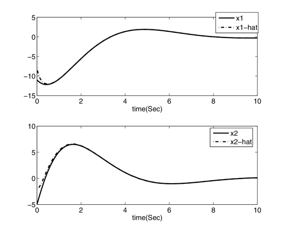
Figure 1: The true and estimated states of the example

The values of $\gamma^{*}$, $\mu^{*}$ and $\bar{\sigma}(L)$, and the optimal trade-off curve between $\gamma^{*}$ and $\mu^{*}$ over the range of $\lambda$ when the decay rate is fixed ($\beta=0.35$) are shown in figure 2.

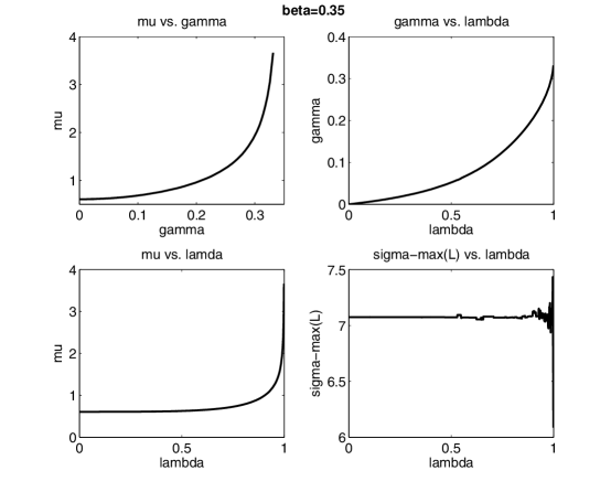
Figure 2: $\gamma^{*}$, $\mu^{*}$ and $\bar{\sigma}(L)$, and the optimal trade-off curve

The optimal surfaces of $\gamma^{*}$, $\mu^{*}$ and $\bar{\sigma}(L)$ over the range of $\lambda$ when the decay rate is variable are shown in figures 3, 4 and 5, respectively. The maximum value of $\gamma^{*}$ is 0.34 obtained when $\lambda=1$. In the range of $0\leq\lambda\leq 1$ and $0\leq\beta\leq 0.8$, the norm of $L$ is almost constant. As $\beta$ increases over 0.8, $\bar{\sigma}(L)$ rapidly increases and for $\beta=1.2$, the LMIs are infeasible.

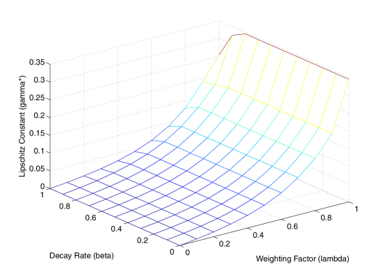
Figure 3: The optimal surface of $\gamma^{*}$

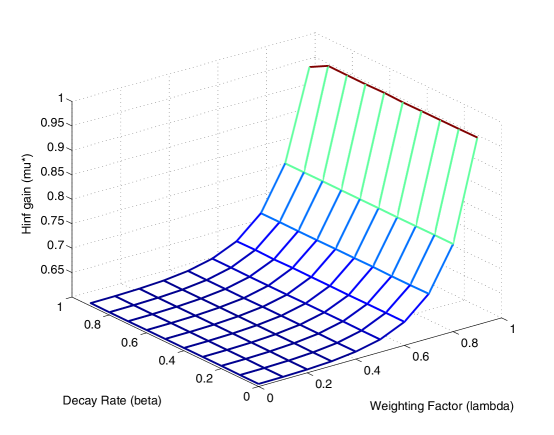
Figure 4: The optimal surface of $\mu^{*}$

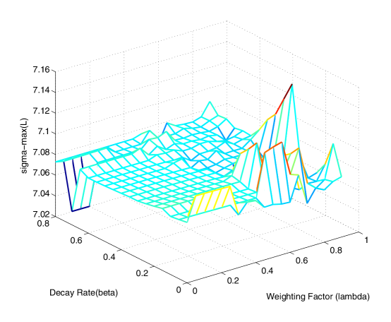
Figure 5: The optimal surface of $\bar{\sigma}(L)$

6 Conclusion

A new nonlinear $H_{\infty}$ observer design method for a class of Lipschitz nonlinear uncertain systems is proposed through LMI optimization. The developed LMIs are linear both in the admissible Lipschitz constant and the disturbance attenuation level allowing both two be an LMI optimization variable. The combined performance of the two optimality criterions is optimized using Pareto optimization. The achieved $H_{\infty}$ observer guarantees asymptotic stability of the error dynamics with a prespecified decay rate (exponential convergence) and is robust against Lipschitz additive nonlinear uncertainty as well as time-varying parametric uncertainty. Explicit bounds on the nonlinear uncertainty are derived through norm-wise and element-wise analysis.

References

- [1] Masoud Abbaszadeh and Horacio J. Marquez. Robust observer design for a class of continuous-time Lipschitz nonlinear systems. Proceedings of the 45th IEEE Conference on Decision and Control, San Diego, U.S.A., pages 3895–3900, 2006.
- [2] Masoud Abbaszadeh and Horacio J Marquez. LMI optimization approach to robust filtering for discrete-time nonlinear uncertain systems. In American Control Conference, 2008, pages 1905–1910, 2008.
- [3] Masoud Abbaszadeh and Horacio J. Marquez. Robust observer design for sampled-data Lipschitz nonlinear systems with exact and Euler approximate models. Automatica, 44(3):799–806, 2008.
- [4] Masoud Abbaszadeh and Horacio J Marquez. Robust filtering for lipschitz nonlinear systems via multiobjective optimization. Journal of Signal & Information Processing, 1(1):24–34, 2010.
- [5] Masoud Abbaszadeh and Horacio J Marquez. A generalized framework for robust nonlinear filtering of lipschitz descriptor systems with parametric and nonlinear uncertainties. Automatica, 48(5):894–900, 2012.
- [6] S. Boyd, L. El Ghaoui, E. Feron, and V. Balakrishnan. Linear matrix inequalities in system and control theory. SIAM, PA, 1994.
- [7] S. Boyd and L. Vandenberghe. Convex Optimization. Cambrige University Press, 2004.
- [8] X. Chen, T. Fukuda, and K. D. Young. A new nonlinear robust disturbance observer. Systems and Control Letters, 41(3):189–199, 2000.
- [9] Carlos E. de Souza, Lihua Xie, and Youyi Wang. filtering for a class of uncertain nonlinear systems. Systems and Control Letters, 20(6):419–426, 1993.
- [10] R. A. Horn and C. R. Johnson. Matrix Analysis. Cambrige University Press, 1985.
- [11] R. A. Horn and C. R. Johnson. Topics in Matrix Analysis. Cambrige University Press, 1991.
- [12] A. Howell and J. K. Hedrick. Nonlinear observer design via convex optimization. Proceedings of the American Control Conference, 3:2088–2093, 2002.
- [13] Pramod P. Khargonekar, Ian R. Petersen, and Kemin Zhou. Robust stabilization of uncertain linear systems: Quadratic stabilizability and control theory. IEEE Transactions on Automatic Control, 35(3):356–361, 1990.
- [14] G. Lu and D. W. C. Ho. Robust observer for nonlinear discrete systems with time delay and parameter uncertainties. IEE Proceedings: Control Theory and Applications, 151(4):439–444, 2004.
- [15] H. J. Marquez. Nonlinear Control Systems: Analysis and Design. Wiley, NY, 2003.
- [16] W. M. McEneaney. Robust filtering for nonlinear systems. Systems and Control Letters, 33(5):315–325, 1998.
- [17] S. K. Nguang and M. Fu. Robust nonlinear filtering. Automatica, 32(8):1195–1199, 1996.
- [18] A. M. Pertew, H. J. Marquez, and Q. Zhao. observer design for Lipschitz nonlinear systems. IEEE Transactions on Automatic Control, 51(7):1211–1216, 2006.
- [19] Youyi Wang, Lihua Xie, and Carlos E. de Souza. Robust control of a class of uncertain nonlinear systems. Systems and Control Letters, 19(2):139–149, 1992.
- [20] S. Xu and J. Lam. On filtering for a class of uncertain nonlinear neutral systems. Circuits, Systems, and Signal Processing, 23(3):215–230, 2004.
- [21] Shengyuan Xu. Robust filtering for a class of discrete-time uncertain nonlinear systems with state delay. IEEE Transactions on Circuits and Systems I: Fundamental Theory and Applications, 49(12):1853 – 1859, 2002.
- [22] Shengyuan Xu and Paul Van Dooren. Robust filtering for a class of non-linear systems with state delay and parameter uncertainty. International Journal of Control, 75(10):766–774, 2002.
- [23] C. Yung, Y. Li, and H. Sheu. filtering and solution bound for non-linear systems. International Journal of Control, 74(6):565–570, 2001.