Atmospheres and radiating surfaces of neutron stars

Abstract

The early 21st century witnesses a dramatic rise in the study of thermal radiation of neutron stars. Modern space telescopes have provided a wealth of valuable information which, when properly interpreted, can elucidate the physics of superdense matter in the interior of these stars. This interpretation is necessarily based on the theory of formation of neutron star thermal spectra, which, in turn, is based on plasma physics and on the understanding of radiative processes in stellar photospheres. In this paper, the current status of the theory is reviewed with particular emphasis on neutron stars with strong magnetic fields. In addition to the conventional deep (semi-infinite) atmospheres, radiative condensed surfaces of neutron stars and ”thin” (finite) atmospheres are considered.

PACS numbers: 97.60.Jd, 97.10.Ex, 97.10.Ld

1 Introduction

Neutron stars are the most compact of all stars ever observed: with a typical mass $M\sim(1$ – $2)\,M_{\odot}$, where $M_{\odot}=2\times 10^{33}$ g is the solar mass, their radius is $R\approx 10$ – 13 km. The mean density of such star is $\sim 10^{15}$ g cm^-3, i.e., a few times the typical density of a heavy atomic nucleus $\rho_{0}=2.8\times 10^{14}$ g cm^-3. The density at the neutron-star center can exceed $\rho_{0}$ by an order of magnitude. Such matter cannot be obtained in a laboratory, and its properties still remain to be clarified. Even its composition is not completely known, because neutron stars, despite their name, consist not only of neutrons. There are a variety of theoretical models to describe neutron-star matter (see [1] and references therein), and a choice in favor of one of them requires an analysis and interpretation of relevant observational data. Therefore, observational manifestations of the neutron stars can be used for verification of theoretical models of matter in extreme conditions [2]. Conversely, the progress in studying the extreme conditions of matter provides prerequisites for construction of neutron-star models and adequate interpretation of their observations. A more general review of these problems is given in [3]. In this paper, I will consider more closely one of them, namely the formation of thermal electromagnetic radiation of neutron stars.

Neutron stars are divided into accreting and isolated ones. The former ones accrete matter from outside, while an accretion onto the latter ones is negligible. There are also transiently accreting neutron stars (X-ray transients), whose active periods (with accretion) alternate with quiescent periods, during which the accretion almost stops. The bulk of radiation from the accreting neutron stars is due to the matter being accreted, which forms a circumstellar disk, accretion flows, and a hot boundary layer at the surface. At contrast, a significant part of radiation from isolated neutron stars, as well as from the transients in quiescence, appear to originate at the surface or in the atmosphere. To interpret this radiation, it is important to know the properties of the envelopes that contribute to the spectrum formation. On the other hand, comparison of theoretical predictions with observations may be used to deduce these properties and to verify theoretical models of the dense magnetized plasmas that constitute the envelopes.

We will consider the outermost envelopes of the neutron stars – their atmospheres. A stellar atmosphere is the plasma layer in which the electromagnetic spectrum is formed and from which the radiation escapes into space without significant losses. The spectrum contains a valuable information on the chemical composition and temperature of the surface, intensity and geometry of the magnetic field, as well as on the stellar mass and radius.

In most cases, the density in the atmosphere grows with increasing depth gradually, without a jump, but stars with a very low temperature or a superstrong magnetic field can have a solid or liquid surface. Formation of the spectrum with presence of such a surface will also be considered in this paper.

2 Basic characteristics of neutron stars

2.1 Masses and radii

The relation between mass $M$ and radius $R$ of a star is given by a solution of the hydrostatic equilibrium equation for a given equation of state (EOS), that is the dependence of pressure $P$ on density $\rho$ and temperature $T$, along with the thermal balance equation. The pressure in neutron star interiors is mainly produced by highly degenerate fermions with Fermi energy $\epsilon_{\mathrm{F}}\gg k_{\mathrm{B}}T$ ($k_{\mathrm{B}}$ is the Boltzmann constant), therefore one can neglect the $T$-dependence in calculations of $R(M)$. For the central regions of typical neutron stars, where $\rho\gtrsim\rho_{0}$, the EOS and even composition of matter is not well known because of the lack of the precise relativistic many-body theory of strongly interacting particles. Instead of the exact theory, there are many approximate models, which give a range of theoretical EOSs and, accordingly, $R(M)$ relations (see, e.g., Chapt. 6 of [1]).

For a star to be hydrostatically stable, the density at the stellar center has to increase with increasing mass. This condition is satisfied in a certain interval $M_{\mathrm{min}}<M<M_{\mathrm{max}}$. The minimum neutron-star mass is rather well established, $M_{\mathrm{min}}\approx 0.1\,M_{\odot}$ [4]. The maximum mass until recently was allowed to lie in a wide range $M_{\mathrm{max}}\sim(1.5$ – $2.5)\,M_{\odot}$ by competing theories (see, e.g., Table 6.1 in Ref. [1]), but the discoveries of neutron stars with masses $M=1.97\pm 0.04\,M_{\odot}$ [5] and $2.01\pm 0.04\,M_{\odot}$ [6] showed that $M_{\mathrm{max}}>2\,M_{\odot}$.

Simulations of formation of neutron stars [7, 8] show that $M$, as a rule, exceeds $M_{\odot}$, the most typical values being in the range (1.2 – $1.6)\,M_{\odot}$. Observations generally agree with these conclusions. Masses of several pulsars in double compact-star systems are known with a high accuracy ($\lesssim 1$%) due to the measurements of the General Relativity (GR) effects on their orbital parameters. All of them lie in the interval from $1.3\,M_{\odot}$ to $2.0\,M_{\odot}$ [9, 5, 6]. Masses of other neutron stars that have been measured with an accuracy better than 10% cover the range $M_{\odot}\lesssim M\lesssim 2\,M_{\odot}$ [1, 10].

Were radius $R$ and mass $M$ known precisely for at least a single neutron star, it would probably ensure selecting one of the nuclear-matter EOSs as the most realistic one. However, the current accuracy of measurements of neutron star radii leaves much to be desired.

2.2 Magnetic fields

Most of the known neutron stars possess strong magnetic fields, unattainable in the terrestrial laboratories. Gnedin and Sunyaev [11] pointed out that spectra of such stars can contain the resonant electron-cyclotron line. Its detection allows one to obtain magnetic field $B$ by measurement of the cyclotron frequency $\omega_{\mathrm{c}}=eB/(m_{\mathrm{e}}c)$, where $m_{\mathrm{e}}$ and $(-e)$ are the electron mass and charge, and $c$ is the speed of light in vacuum (here and hereafter we use the Gaussian system of units). The discovery of the cyclotron line in the spectrum of the X-ray pulsar in the binary system Hercules X-1 [12] gave a striking confirmation of this idea. About 20 accreting X-ray pulsars are currently known to reveal the electron cyclotron line and sometimes several its harmonics at energies of tens keV, corresponding to $B\approx(1$ – $4)\times 10^{12}$ G (e.g., [13, 14, 15, 16]).

An alternative interpretation of the observed lines was suggested in [17]. It assumes an anisotropic distribution of electron velocities in a collisionless shock wave with large Lorentz factors (the ratios of the total electron energy to $m_{\mathrm{e}}c^{2}=511$ keV), $\gamma_{\mathrm{r}}\sim 40$. The radiation frequency of such electrons strongly increases because of the relativistic Doppler effect, which enables an explanation of the observed position of the line by a much weaker field than in the conventional interpretation. It was noted in Ref. [18] that the small width of the lines (from one to several keV [13]) is difficult to accommodate in this model. It also leaves unexplained, why the position of the line is usually almost constant. For example, the measured cyclotron energy of the accreting X-ray pulsar A 0535+26 remains virtually constant while its luminosity changes by two orders of magnitude [19].

On the other hand, most X-ray pulsars do exhibit a dependence, albeit weak, of the observed line frequency on luminosity [20]. In order to explain this dependence, a model was suggested in [21], assuming that the cyclotron lines are formed by reflection from the stellar surface, irradiated by the accretion column. When luminosity increases, the bulk of reflection occurs at lower magnetic latitudes, where the field is weaker than at the pole, therefore the cyclotron frequency becomes smaller. This model, however, does not explain the cases where the observed frequency increases with luminosity and, as noted in [22], it does not reproduce X-ray pulses at large luminosities.

A quantitative description of all observed dependences of the cyclotron frequency on luminosity is developed in Ref. [20], based on a physical model of cyclotron-line formation in the accretion column. The height of the region above the surface, where the lines are formed, $h\sim(10^{-3}$ – $10^{-1})R$, correlates with luminosity, the correlation being positive or negative depending on the luminosity value. Then the line is centered at the frequency $\omega_{\mathrm{c}}/(1+h/R)^{3}$, where $\omega_{\mathrm{c}}$ is the cyclotron frequency at the base of the accretion column. In [22], variations of a polar cap diameter and a beam pattern were additionally taken into account, which has allowed the author to explain variations in the width and depth of the observed lines in addition to their frequencies.

When cyclotron features are not identified in the spectrum, one has to resort to indirect estimates of the magnetic field. For the isolated pulsars, the most widely used estimate is based on the expression

$$B\approx 3.2\times 10^{19}\,C\,\sqrt{\mathcal{P}\dot{\mathcal{P}}}\textrm{~{}~{}G},$$ (1)

where $\mathcal{P}$ is the period in seconds, $\dot{\mathcal{P}}$ is the period time derivative, and $C$ is a coefficient, which depends on stellar parameters. For the rotating magnetic dipole in vacuo [23] $C=R_{6}^{-3}\,(\sin\alpha)^{-1}\,\sqrt{I_{45}}$, where $R_{6}\equiv R/(10^{6}\mbox{~{}cm})$, $I_{45}$ is the moment of inertia in units of $10^{45}$ g cm², and $\alpha$ is the angle between the magnetic and rotational axes. In this case Eq. (1) gives the magnetic field strength at the pole. If $M\approx(1$ – 2) $M_{\odot}$, then $R_{6}\approx 1.0$ – 1.3 and $I_{45}\approx 1$ – 3 (see [1]). For estimates, one usually sets $C=1$ in Eq. (1) (e.g., [24]).

A real pulsar strongly differs from a rotating magnetic dipole, because its magnetosphere is filled with plasma, carrying electric charges and currents (see reviews [25, 26, 27, 28] and recent papers [29, 30, 31]). According to the model by Beskin et al. [32, 33], the magnetodipole radiation is absent beyond the magnetosphere, while the slowdown of rotation is provided by the current energy losses. However, the the relation between $B$ and $\mathcal{P}\dot{\mathcal{P}}$ remains similar. Results of numerical simulations of plasma behavior in the pulsar magnetosphere can be approximately described by Eq. (1) with $C\approx 0.8R_{6}^{-3}\,(1+\sin^{2}\alpha)^{-1/2}\,\sqrt{I_{45}}$ [34]. As shown in [28], this result does not contradict to the model [32, 33].

Magnetic fields of the ordinary radio pulsars are distributed near $B\sim 10^{12}$ G [35], the “recycled” millisecond pulsars have $B\sim(10^{8}$ – $10^{10})$ G [35, 36, 37], and the fields of magnetars much exceed $10^{13}$ G [38, 39]. According to the most popular point of view, anomalous X-ray pulsars (AXPs) and soft gamma repeaters (SGRs) [38, 39, 40, 41, 42] are magnetars. For these objects, the estimate (1) most often (although not always) gives $B\sim 10^{14}$ G, but in order to explain their energy balance, magnetic fields reaching up to $B\sim 10^{16}$ – $10^{17}$ G in the core at the birth of the star are considered (see [43] and references therein). Numerical calculations [44] show that magnetorotational instability in the envelope of a supernova, that is a progenitor of a neutron star, can give rise to nonstationary magnetic fields over $10^{15}$ G. It is assumed that in addition to the poloidal magnetic field at the surface, the magnetars may have much stronger toroidal magnetic field embedded in deeper layers [45, 46]. Indeed, for a characteristic poloidal component $B_{\mathrm{pol}}$ of a neutron-star magnetic field to be stable, a toroidal component $B_{\mathrm{tor}}$ must be present, such that, by order of magnitude, $B_{\mathrm{pol}}\lesssim B_{\mathrm{tor}}\lesssim 10^{16}\mbox{~{}G}\sqrt{B_{\mathrm{pol}}/(10^{13}\mbox{~{}G})}$ [47]. Meanwhile, there is increasing evidence for the absence of a clear distinction between AXPs and SGRs [48], as well as between these objects and other neutron stars [49, 41, 42]. There has even appeared the paradoxical name “a low-field magnetar,” applied to those AXPs and SGRs that have $B\ll 10^{14}$ G (e.g., [50, 51], and references therein).

For the majority of isolated neutron stars, the magnetic-field estimate (1) agrees with other data (e.g., with observed properties of the bow shock nebula in the vicinity of the star [52]). For AXPs and SGRs, however, one cannot exclude alternative models, which do not involve superstrong fields but assume weak accretion on a young neutron star with $B\sim 10^{12}$ G from a circumstellar disk, which could remain after the supernova burst [53, 54, 56, 55]. There is also a “drift model”, which suggests that the observed AXP and SGR periods equal not to rotation periods but to periods of drift waves, which affect the magnetic-lines curvature and the direction of radiation in the outer parts of magnetospheres of neutron stars with $B\sim 10^{12}$ G [57, 58]. Another model suggests that the AXPs and SGRs are not neutron stars at all, but rather massive ($M>M_{\odot}$) rapidly rotating white dwarfs with $B\sim 10^{8}$ – $10^{9}$ G ([59] and references therein).

The measured neutron-star magnetic fields are enormous by terrestrial scales, but still far below the theoretical upper limit. An order-of-magnitude estimate of this limit can be obtained by equating the gravitational energy of the star to its electromagnetic energy [60]. For neutron stars, such estimate gives the limiting field $B_{\mathrm{max}}\sim 10^{18}$ – $10^{19}$ G [61]. Numerical simulations of hydrostatic equilibrium of magnetized neutron stars show that $B_{\mathrm{max}}\lesssim 10^{18}$ G [62, 63, 64, 65]. Still stronger magnetic fields imply so intense electric currents that their interaction would disrupt the star. Note in passing that the highest magnetic field that can be accommodated in quantum electrodynamics (QED) is, by order of magnitude, $[m_{\mathrm{e}}^{2}c^{3}/(e\hbar)]\exp(\pi^{3/2}/\sqrt{\alpha_{\mathrm{f}}})\approx 10^{42}$ G [66], where $\alpha_{\mathrm{f}}=e^{2}/(\hbar c)\approx 1/137$ is the fine structure constant, and $\hbar$ is the Planck constant divided by $2\pi$.

We will see below that magnetic fields $B\gtrsim 10^{11}$ G strongly affect the most important characteristics of neutron-star envelopes. These effects are particularly pronounced at radiating surfaces and in atmospheres, which are the main subject of the present review.

2.3 General Relativity effects

The significance of the GR effects for a star is quantified by the compactness parameter

$$x_{\mathrm{g}}=r_{g}/R,$$ (2)

where

$$r_{g}=2GM/c^{2}\approx 2.95\,M/M_{\odot}\textrm{ km}$$ (3)

is the Schwarzschild radius, and $G$ is the gravitational constant. The compactness parameter of a typical neutron star lies between 1/5 and 1/2, that is not small (for comparison, the Sun has $x_{\mathrm{g}}=4.24\times 10^{-6}$). Hence, the GR effects are not negligible. Two important consequences follow: first, the quantitative theory of neutron stars must be wholly relativistic; second, observations of neutron stars open up a unique opportunity for measuring the GR effects and verification of the GR predictions.

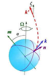
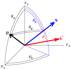
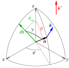
Fig. 1: Left panel: an illustration of the gravitational light-bending near a neutron star; $\mathbf{n}$ is the normal to the surface at a radiating point, $\bm{k}$ is the wave vector of an emitted ray in the local reference frame, $\bm{k^{\prime}}$ is the wave vector in the observer’s reference frame. In addition, the stellar rotation vector $\mathbf{\Omega}$ and magnetic moment $\bm{m}$ are shown. The angles formed by the rotation axis with the magnetic moment ($\alpha$) and with the line of sight ($\zeta$) are indicated. Middle panel: wave vectors $\bm{k}$, $\bm{k^{\prime}}$, and the magnetic field vector $\bm{B}$ in the local reference frame $(x_{\mathrm{n}}y_{\mathrm{n}}z_{\mathrm{n}})$ with the $z$-axis along $\mathbf{n}$ and the $x$-axis along the projection of $\bm{B}$ on the surface; $\theta_{\mathrm{n}}$ is the angle between $\bm{B}$ and $\mathbf{n}$, $\theta_{k}$ and $\theta$ are the angles between the wave vectors and the normal, $\theta_{B}$ is the angle between the ray and the magnetic field, and $\varphi_{k}$ is the azimuth. Right panel: vectors $\mathbf{n}$, $\bm{k}$, $\bm{k^{\prime}}$, and $\hat{\mathbf{m}}\equiv\bm{m}/|\bm{m}|$ in the coordinate system $(xyz)$ with the $z$-axis along the line of sight and the $x$-axis along the projection of $\bm{m}$ on the picture plane; $\theta_{\mathrm{m}}$ is the angle between $\bm{m}$ and the line of sight, $\gamma$ is the angle between $\mathbf{n}$ and $\bm{m}$, and $\varphi$ is the azimuth.

In GR, gravity at the stellar surface is determined by the equation

$$g=\frac{GM}{R^{2}\,\sqrt{1-x_{\mathrm{g}}}}\approx\frac{1.328\times 10^{14}}{\sqrt{1-x_{\mathrm{g}}}}\,\frac{M/M_{\odot}}{\,R_{6}^{2}}\textrm{ cm s}^{-2}.$$ (4)

Stellar hydrostatic equilibrium is governed by the Tolman-Oppenheimer-Volkoff equation (corrections due to the rotation and magnetic fields are negligible for the majority of neutron stars):

$$\frac{\mathrm{d}P}{\mathrm{d}r}=-\left(1+\frac{P}{\rho c^{2}}\right)\,\left(1+\frac{4\pi r^{3}P}{M_{r}c^{2}}\right)\,\left(1-\frac{2GM_{r}}{rc^{2}}\right)^{-1/2},$$ (5)

where $r$ is the radial coordinate measured from the stellar center, and $M_{r}$ is the mass inside a sphere of radius $r$.

The photon frequency, which equals $\omega$ in the local inertial reference frame, undergoes a redshift to a smaller frequency $\omega_{\infty}$ in the remote observer’s reference frame. Therefore a thermal spectrum with effective temperature $T_{\mathrm{eff}}$, measured by the remote observer, corresponds to a lower effective temperature

$$T_{\mathrm{eff}}^{\infty}=T_{\mathrm{eff}}/(1+z_{g}),$$ (6)

where

$$z_{g}\equiv\omega/\omega_{\infty}-1=(1-x_{\mathrm{g}})^{-1/2}-1$$ (7)

is the redshift parameter. Here and hereafter the symbol $\infty$ indicates that the given quantity is measured at a large distance from the star and can differ from its value near the surface.

Along with the radius $R$ that is determined by the equatorial length $2\pi R$ in the local reference frame, one often considers an apparent radius for a remote observer,

$$R_{\infty}=R\,(1+z_{g}).$$ (8)

With decreasing $R$, $z_{g}$ increases so that the apparent radius has a minimum, $\min R_{\infty}\approx 12$ – 14 km ([1], Chapt. 6).

The apparent photon luminosity $L_{\mathrm{ph}}^{\infty}$ and the luminosity in the stellar reference frame $L_{\mathrm{ph}}$ are determined by the Stefan-Boltzmann law

$$L_{\mathrm{ph}}^{\infty}=4\pi\sigma_{\mathrm{SB}}\,R_{\infty}^{2}\,(T_{\mathrm{eff}}^{\infty})^{4},\quad L_{\mathrm{ph}}=4\pi\sigma_{\mathrm{SB}}\,R^{2}T_{\mathrm{eff}}^{4}$$ (9)

with $\sigma_{\mathrm{SB}}=\pi^{2}k_{\mathrm{B}}^{4}/(60\hbar^{3}c^{2})$. According to (6) – (8), they are interrelated as

$$L_{\mathrm{ph}}^{\infty}=(1-x_{\mathrm{g}})\,L_{\mathrm{ph}}=L_{\mathrm{ph}}/(1+z_{g})^{2}.$$ (10)

In the absence of the perfect spherical symmetry, it is convenient to define a local effective surface temperature $T_{\mathrm{s}}$ by the relation

$$F_{\mathrm{ph}}(\theta,\varphi)=\sigma_{\mathrm{SB}}T_{\mathrm{s}}^{4},$$ (11)

where $F_{\mathrm{ph}}$ is the local radial flux density at the surface point, determined by the polar angle ($\theta$) and azimuth ($\varphi$) in the spherical coordinate system. Then

$$L_{\mathrm{ph}}=\int_{0}^{\pi}\sin\theta\,\mathrm{d}\theta\int_{0}^{2\pi}\mathrm{d}\varphi\,R^{2}F_{\mathrm{ph}}(\theta,\varphi)\,.$$ (12)

The same relation connects the apparent luminosity $L_{\mathrm{ph}}^{\infty}$ (10) with the apparent flux $F_{\mathrm{ph}}^{\infty}=\sigma_{\mathrm{SB}}\,(T_{\mathrm{s}}^{\infty})^{4}$ in the remote system, in accord with the relation $T_{\mathrm{s}}^{\infty}=T_{\mathrm{s}}/(1+z_{\mathrm{g}})$ analogous to (6).

The expressions (6), (8) and (10) agree with the concepts of the light ray bending and time dilation near a massive body. If the angle between the wave vector $\bm{k}$ and the normal to the surface $\mathbf{n}$ at the emission point is $\theta_{k}$, then the observer receives a photon whose wave vector $\bm{k^{\prime}}$ makes an angle $\theta>\theta_{k}$ with $\mathbf{n}$ (Fig. 1). The rigorous theory of the influence of the light bending near a star on its observed spectrum has been developed in [67] and cast in a convenient form in [68, 69]. The simple approximation [70]

$$\cos\theta_{k}=x_{\mathrm{g}}+(1-x_{\mathrm{g}})\cos\theta$$ (13)

is applicable at $x_{\mathrm{g}}<0.5$ with an error within a few percent. At $\cos\theta_{k}<x_{\mathrm{g}}$, Eq. (13) gives $\theta>\pi/2$, as if the observer looked behind the neutron-star horizon. In particular, for a star with a dipole magnetic field and a sufficiently large inclination angle $\theta_{\mathrm{m}}$ of the dipole moment vector $\bm{m}$ to the line of site, the observer can see the two opposite magnetic poles at once. Clearly, such effects should be taken into account while comparing theoretical neutron-star radiation models with observations.

Let $I_{\omega}$ be the specific intensity per unit circular frequency (if $I_{\nu}$ is the specific intensity per unit frequency, then $I_{\omega}=I_{\nu}/(2\pi)$; see [71]). A contribution to the observed radiation flux density from a small piece of the surface $\mathrm{d}\mathcal{A}$ in the circular frequency interval $[\omega,\omega+\mathrm{d}\omega]$ equals [72, 73]

$$\mathrm{d}F_{\omega_{\infty}}^{\infty}=I_{\omega}(\bm{k})\,\cos\theta_{k}\left|\frac{\mathrm{d}\cos\theta_{k}}{\mathrm{d}\cos\theta}\right|\,\frac{\mathrm{d}\mathcal{A}}{D^{2}}\,(1-x_{\mathrm{g}})\,\mathrm{d}\omega,$$ (14)

where $\mathrm{d}\omega=(1+z_{g})\,\mathrm{d}\omega_{\infty}$. Here and hereafter we assume that the rotational velocity of the patch $\mathrm{d}\mathcal{A}$ is much smaller than the speed of light. If this condition is not satisfied, then the right-hand side of Eq. (14) should be multiplied by $(\cos\tilde{\theta}_{k}/\cos\theta_{k})^{4}$, where $\tilde{\theta}_{k}$ is the angle between the surface normal and the wave vector in the reference frame, comoving with the patch $\mathrm{d}\mathcal{A}$ at the moment of radiation [72, 73]. For a spherical star, Eqs. (13), (14) give

$$F_{\omega_{\infty}}^{\infty}=(1-x_{\mathrm{g}})^{3/2}\frac{R^{2}}{D^{2}}\int I_{\omega}(\bm{k};\theta,\varphi)\,\cos\theta_{k}\sin\theta\,\mathrm{d}\theta\,\mathrm{d}\varphi,$$ (15)

where the integration is restricted by the condition $\cos\theta_{k}>0$.

The magnetic field is also distorted by the space curvature in the GR. For the uniform and dipole fields, this distortion is described by Ginzburg & Ozernoi [74]. In the dipole field case, the magnetic vector is

$$\bm{B}=B_{\textrm{p}}\,(\mathbf{n}\cdot\hat{\mathbf{m}})\,\mathbf{n}+B_{\textrm{eq}}\,\big{[}(\mathbf{n}\cdot\hat{\mathbf{m}})\,\mathbf{n}-\hat{\mathbf{m}}\big{]},$$ (16)

where $\hat{\mathbf{m}}=\bm{m}/|\bm{m}|$ is the magnetic axis direction, $B_{\textrm{eq}}$ and $B_{\textrm{p}}$ are the equatorial and polar field strengths, respectively, and their ratio equals

$$\frac{B_{\textrm{eq}}}{B_{\textrm{p}}}=\frac{x_{\mathrm{g}}^{2}/2-(1-x_{\mathrm{g}})\ln(1-x_{\mathrm{g}})-x_{\mathrm{g}}}{[\ln(1-x_{\mathrm{g}})+x_{\mathrm{g}}+x_{\mathrm{g}}^{2}/2]\sqrt{1-x_{\mathrm{g}}}}.$$ (17)

In the limit of flat geometry ($x_{\mathrm{g}}\to 0$) $B_{\textrm{eq}}\to B_{\textrm{p}}/2$, but in general $B_{\textrm{eq}}/B_{\textrm{p}}>1/2+x_{\mathrm{g}}/8$.

Muslimov & Tsygan [75] obtained expansions of the components of a poloidal magnetic field vector $\bm{B}$ over the scalar spherical harmonics near a static neutron star beyond the dipole approximation. Equations (16) and (17) are a particular case of this expansion. Petri [76] developed a technique of expansion of electromagnetic fields around a rotating magnetized star over vector spherical harmonics, which allows one to find a solution of the Maxwell equations in the GR for an arbitrary multipole component of the magnetic field. In this case, the solutions for a nonrotating star in the GR [75] and for a rotating dipole in the flat geometry [23] are reproduced as particular cases.

2.4 Measuring masses and radii by thermal spectrum

Information on the mass and radius of a neutron star can be obtained from its thermal spectrum. To begin with, let us consider the perfect blackbody radiation whose spectrum is described by the Planck function

$$\mathcal{B}_{\omega,T}=\frac{\hbar\omega^{3}}{4\pi^{3}c^{2}}\,\frac{1}{\exp[\hbar\omega/k_{\mathrm{B}}T]-1},$$ (18)

and neglect interstellar absorption and nonuniformity of the surface temperature distribution. The position of the spectral maximum $\hbar\omega_{\mathrm{max}}=2.8k_{\mathrm{B}}T$ gives us the effective temperature $T_{\mathrm{eff}}^{\infty}$, and the measured intensity gives the total flux density $F_{\mathrm{bol}}$ that reaches the observer. If the star is located at distance $D$, then its apparent photon luminosity is $L_{\mathrm{ph}}^{\infty}=4\pi D^{2}F_{\mathrm{bol}}$, and Eq. (9) yields $R_{\infty}$.

In reality, comparison of theoretical and measured spectra depends on a larger number of parameters. First, the spectrum is modified by absorption in the interstellar matter. The effect of the interstellar gas on the X-ray part of the spectrum is approximately described by factor $\exp[-(N_{\mathrm{H}}/10^{21}\mbox{~{}cm}^{-2})\,(\hbar\omega/0.16\mbox{~{}keV})^{-8/3}]$, where $N_{\mathrm{H}}$ is the hydrogen column density on the line of sight [77]. Thus one can evaluate $N_{\mathrm{H}}$ from an analysis of the spectrum. If $D$ is unknown, one can try to evaluate it assuming a typical interstellar gas density for the given Galaxy region and using $D$ as a fitting parameter.

Second, the temperature distribution can be nonuniform over the stellar surface. For example, at contrast to the cold poles of the Earth, the pulsars have heated regions near their magnetic poles, “hot polar caps.” The polar caps of accreting neutron stars with strong magnetic fields are heated by matter flow from a companion star through an accretion disk and accretion column (see [78, 79] and references therein). The polar caps of isolated pulsars and magnetars are heated by the current of charged particles, created in the magnetosphere and accelerated by the electric field along the magnetic field lines (see the reviews [25, 80, 28], papers [81, 82], and references therein). The thermal spectrum of such neutron stars is sometimes represented as consisting of two components, one of them being related to the heated region and the other to the rest of the surface, each with its own value of the effective temperature and effective apparent radius of the emitting area (e.g., [83]). Besides, variable strength and direction of the magnetic field over the surface affect the thermal conductivity of the envelope. Hence, the temperature $T_{\mathrm{s}}$ of a cooling neutron star outside the polar regions is also nonuniform (see, e.g., [84, 85]).

Finally, a star is not a perfect blackbody, therefore its radiation spectrum differs from the Planck function. Spectral modeling is a complex task, which includes solving equations of hydrostatic equilibrium, energy balance, and radiative transfer (below we will consider it in more detail). Coefficients of these equations depend on chemical composition of the atmosphere, effective temperature, gravity, and magnetic field. Making different assumptions about the chemical composition, $M$, $R$, $T_{\mathrm{eff}}$, and $B$ values, and about distributions of $T_{\mathrm{s}}$ and $\bm{B}$ over the surface, one obtains different model spectra. Comparison of these spectra with the observed spectrum yields an evaluation of acceptable values of the parameters. With the known shape of the spectrum, one can calculate $F_{\mathrm{bol}}$ and evaluate $R_{\infty}$ using Eq. (9). Identification of spectral features may provide $z_{g}$. A simultaneous evaluation of $z_{g}$ and $R_{\infty}$ allows one to calculate $M$ from Eqs. (2), (3), (7), and (8). This method of mass and radius evaluation requires a reliable theoretical description of the envelopes that affect the surface temperature and radiation spectrum.

2.5 Neutron-star envelopes

Not only the superdense core of a neutron star, but also the envelopes are mostly under conditions unavailable in the laboratory. By the terrestrial standards, they are characterized by superhigh pressures, densities, temperatures, and magnetic fields. The envelopes differ by their composition, phase state, and their role in the evolution and properties of the star.

In the deepest envelopes, just above the core of a neutron star, matter forms a neutron liquid with immersed atomic nuclei and electrons. In these layers, the neutrons and electrons are strongly degenerate, and the nuclei are neutron-rich, that is, their neutron number can be several times larger than the proton number, so that only the huge pressure keeps such nuclei together. Electrostatic interaction of the nuclei is so strong that they are arranged in a crystalline lattice, which forms the solid stellar crust. There can be a mantle between the crust and the core (though not all of the modern models of the dense nuclear matter predict its existence). Atomic nuclei in the mantle take exotic shapes of extended cylinders or planes [86]. Such matter behaves like liquid crystals [87].

The neutron-star crust is divided into the inner and outer parts. The outer crust is characterized by the absence of free neutrons. The boundary lies at the critical neutron-drip density $\rho_{\mathrm{nd}}$. According to current estimates [88], $\rho_{\mathrm{nd}}=4.3\times 10^{11}$ g cm^-3. With decreasing ion density $n_{\mathrm{i}}$, their electrostatic interaction weakens, and finally a Coulomb liquid becomes thermodynamically stable instead of the crystal. The position of the melting boundary, which can be called the bottom of the neutron-star ocean, depends on temperature and chemical composition of the envelope. If all the ions in the Coulomb liquid have the same charge $Ze$ and mass $m_{\mathrm{i}}=Am_{\mathrm{u}}$, where $m_{\mathrm{u}}=1.66\times 10^{-24}$ g is the atomic mass unit, and if the magnetic field is not too strong, then ion dynamics is determined only by the Coulomb coupling constant $\Gamma_{\mathrm{Coul}}$, that is the typical electrostatic to thermal energy ratio for the ions:

$$\Gamma_{\mathrm{Coul}}=\frac{(Ze)^{2}}{a_{\mathrm{i}}k_{\mathrm{B}}T}=\frac{22.75\,Z^{2}}{T_{6}}\,\left(\frac{\rho_{6}}{A}\right)^{1/3},$$ (19)

where $a_{\mathrm{i}}=(4\pi n_{\mathrm{i}}/3)^{-1/3}$, $T_{6}\equiv T/(10^{6}$ K) and $\rho_{6}\equiv\rho/(10^{6}$ g cm^-3). Given the strong degeneracy, the electrons are often considered as a uniform negatively charged background. In this model, the melting occurs at $\Gamma_{\mathrm{Coul}}=175$ [89]. However, the ion-electron interaction and quantizing magnetic field can shift the melting point by tens percent [89, 90].

The strong gravity drives rapid separation of chemical elements [91, 92, 93, 94, 95]. Results of Refs. [93, 94, 95] can be combined to find that the characteristic sedimentation time for the impurity ions with mass and charge numbers $A^{\prime}$ and $Z^{\prime}$ (that is the time at which the ions pass the pressure scale height $P/\rho g$) in the neutron-star ocean is

$$t_{\mathrm{sed}}\approx\frac{46\,Z^{2.9}{(Z^{\prime})}^{0.3}A^{-1.8}}{A^{\prime}-AZ^{\prime}/Z+\Delta_{T}+\Delta_{\mathrm{C}}}\,\frac{\rho_{6}^{1.3}}{g_{14}^{2}T_{6}^{0.3}}\mbox{~{}~{}days},$$ (20)

where $g_{14}\equiv g/(10^{14}$ cm s${}^{-2})\sim$1 – 3, $\Delta_{T}$ is a thermal correction to the ideal degenerate plasma model [92, 94], and $\Delta_{\mathrm{C}}$ is an electrostatic (Coulomb) correction [94, 95]. The Coulomb correction $\Delta_{\mathrm{C}}\sim 10^{-3}-10^{-2}$ dominates in strongly degenerate neutron-star envelopes (at $\rho\gtrsim 10^{3}$ g cm^-3), and at smaller densities $\Delta_{T}\gtrsim\Delta_{\mathrm{C}}$. Ions with larger $A/Z$ ratios settle faster, while among ions with equal $A/Z$ the heavier ones settle down faster [92, 94, 95]. It follows from (20) that $t_{\mathrm{sed}}$ is small compared with the known neutron-star ages, therefore neutron-star envelopes consist of chemically pure layers separated by transition bands of diffusive mixing.

Especially important is the thermal blanketing envelope that governs the flux density $F_{\mathrm{ph}}$ radiated by a cooling star with a given internal temperature $T_{\mathrm{int}}$. $F_{\mathrm{ph}}$ is mainly regulated by the thermal conductivity in the “sensitivity strip” [96, 97], which plays the role of a “bottleneck” for the heat leakage. Position of this strip depends on the stellar parameters $M$, $R$, $T_{\mathrm{int}}$, magnetic field, and chemical composition of the envelope. Since the heat transport across the magnetic field is hampered, the depth of the sensitivity strip can be different at different places of a star with a strong magnetic field: it lies deeper at the places where the magnetic field is more inclined to the surface [98]. As a rule, the sensitivity strip embraces the deepest layer of the ocean and the upper part of the crust and lies in the interval $\rho\sim 10^{5}$ – $10^{9}$ g cm^-3.

2.6 Atmosphere

With decreasing density, the ion electrostatic energy and electron Fermi energy eventually become smaller than the kinetic ion energy. Then the degenerate Coulomb liquid gives way to a nondegenerate gas. The outer gaseous envelope of a star constitutes the atmosphere. In this paper, we will consider models of quasistationary atmospheres. They describe stellar radiation only in the absence of intense accretion, since otherwise it is formed mainly by an accretion disk or by flows of infalling matter.

It is important that the sensitivity strip, mentioned in § 2.5, always lies at large optical depths. Therefore radiative transfer in the atmosphere almost does not affect the full thermal flux, so that one can model a spectrum while keeping $F_{\mathrm{ph}}$ determined and $T_{\mathrm{s}}$ from a simplified model of heat transport in the atmosphere. Usually such model is based on the Eddington approximation (e.g., [99]). Shibanov et al. [100] verified the high accuracy of this approximation for determination of the full thermal flux from neutron stars with strong magnetic fields.

Atmospheres of ordinary stars are divided into the lower part called photosphere, where radiative transfer dominates, and the the upper atmosphere, whose temperature is determined by processes other than the radiative transfer. Usually the upper atmosphere of neutron stars is thought to be absent or negligible. Therefore one does not discriminate between the notions of atmosphere and photosphere for the neutron stars. In this respect let us note that vacuum polarization in superstrong magnetic fields (see § 6.3) makes magnetosphere birefringent, so that the magnetosphere, being thermally decoupled from radiation propagating from the star to the observer, can still affect this radiation. Thus the magnetosphere can play the role of an upper atmosphere of a magnetar.

Geometric depth of an atmosphere is several millimeters in relatively cold neutron stars and centimeters in relatively hot ones. These scales can be easily obtained from a simple estimate: as well as for the ordinary stars, a typical depth of a neutron-star photosphere is by order of magnitude slightly larger than the barometric height scale, the latter being equal to $k_{\mathrm{B}}T/(m_{\mathrm{i}}g)\approx(0.83/A)\,(T_{6}/g_{14})$ cm. The photosphere depth to the neutron-star radius ratio is only $\sim 10^{-6}$ (for comparison, for ordinary stars this ratio is $\sim 10^{-3}$), which allows one to calculate local spectra neglecting the surface curvature.

The presence of atoms, molecules, and ions with bound states significantly changes the electromagnetic absorption coefficients in the atmosphere, thereby affecting the observed spectra. A question arises, whether the processes of particle creation and acceleration near the surface of the pulsars let them to have a partially ionized atmosphere. According to canonical pulsar models [24, 25, 26], the magnetosphere is divided in the regions of open and closed field lines, the closed-lines region being filled up by charged particles so that the electric field of the magnetosphere charge in the comoving (rotating) reference frame cancels the electric field arising from the rotation of the magnetized star. The photosphere that lies below this part of the magnetosphere is stationary and electroneutral.

At contrast, there is a strong electric field near the surface in the open-line region. This field accelerates the charged particles almost to the speed of light. It is not obvious that these processes do not affect the photosphere, therefore quantitative estimates are needed. Let us define the column density

$$y_{\mathrm{col}}=\int_{r}^{\infty}(1+z_{g})\,\rho(r)\mathrm{d}r,$$ (21)

where the factor $(1+z_{g})$ takes account of the relativistic scale change in the gravitational field. According to [101], in the absence of a strong magnetic field, ultrarelativistic electrons lose their energy mostly to bremsstrahlung at the depth where $y_{\mathrm{col}}\sim 60\mbox{~{}g~{}cm}^{-2}$. As noted by Bogdanov et al. [102], such column density is orders of magnitude larger than the typical density of a nonmagnetic neutron-star photosphere. Therefore, the effect of the accelerated particles reduces to an additional deep heating.

The situation changes in a strong magnetic field. Electron oscillations driven by the electromagnetic wave are hindered in the directions perpendicular to the magnetic field, which thus decreases the coefficients of electromagnetic wave absorption and scattering by the electrons and atoms (§ 6.5). Therefore the strong magnetic field “clarifies” the plasma, that is, the same mean (Rosseland [103, 104]) optical depth $\tau_{\mathrm{R}}$ is reached at a larger density. For a typical neutron star with $B\gtrsim 10^{11}$ G, the condition $\tau_{\mathrm{R}}=3/2$ that is required to have $T(r)=T_{\mathrm{eff}}$ in the Eddington approximation, is fulfilled at the density [105]

$$\rho\sim B_{12}~{}~{}\mbox{g~{}cm${}^{-3}$},$$ (22)

where $B_{12}\equiv B/(10^{12}$ G). Thus the density of the layer where the spectrum is formed increases with growing $B$. At the same time the main mechanism of electron and positron deceleration changes, which is related to Landau quantization (§ 5.1). In the strong magnetic field, the most effective deceleration mechanism is the magneto-Coulomb interaction, which makes the charged particles colliding with plasma ions to jump to excited Landau levels with subsequent de-excitation through synchrotron radiation [106]. The magneto-Coulomb deceleration length is inversely proportional to $B$. An estimate [106] of the characteristic depth of the magneto-Coulomb deceleration of ultrarelativistic electrons in the neutron-star atmosphere can be written as

$$y_{\mathrm{col}}\approx\big{[}(\gamma_{\mathrm{r}}/700)\,Z^{2}\,A^{-3}\,B_{12}^{-2}\big{]}^{0.43}\,T_{6}\mbox{~{}g~{}cm}^{-2},$$ (23)

$\gamma_{\mathrm{r}}\sim 10^{3}$ – $10^{8}$ being the Lorentz factor. One can easily see from (22) and (23) that at $B\gtrsim 3\times 10^{12}$ G the electrons are decelerated by emitting high-energy photons in an optically thin layer. In this case, the magneto-Coulomb radiation constitutes a nonthermal supplement to the thermal photospheric spectrum of the polar cap.

At the intermediate magnetic fields $10^{11}$ G $\lesssim B\lesssim 3\times 10^{12}$ G, the braking of the accelerated particles occurs in the photosphere. Such polar caps require special photosphere models, where the equations of ionization, energy, and radiative balance would take the braking of charged particles into account.

The photospheres can have different chemical compositions. Before the early 1990s, it was commonly believed that the outer layers of a neutron star consist of iron, as it is the most stable chemical element remaining after the supernova burst that gives birth to a neutron star [107]. Nevertheless, the outer envelopes of an isolated neutron star may contain hydrogen and helium because of accretion of interstellar matter [108, 109]. Even if the star is in the ejector regime [110], that is, its rotating magnetosphere throws away the infalling plasma, a small fraction of the plasma still leaks to the surface (see [78] and references therein). Because of the rapid separation of ions in the strong gravitational field (§ 2.5), an accreted atmosphere can consist entirely of hydrogen. In the absence of magnetic field, hydrogen completely fills the photosphere if its column density exceeds $y_{\mathrm{col}}\gtrsim 0.1\mbox{~{}g~{}cm}^{-2}$. In the field $B\sim 10^{14}$ G this happens at $y_{\mathrm{col}}\gtrsim 10^{3}\mbox{~{}g~{}cm}^{-2}$. Even in the latter case an accreting mass of $\sim 10^{-17}M_{\odot}$ would suffice. But if the accretion occurred at the early stage of the stellar life, when its surface temperature was higher than a few MK, then hydrogen could diffuse into deeper and hotter regions where it would be burnt in thermonuclear reactions [111], leaving helium on the surface [112]. The same might happen to helium [111], and then the surface would be left with carbon [113, 94]. Besides, a mechanism of spallation of heavy chemical elements into lighter ones operates in pulsars due to the collisions of the accelerated particles in the open field line regions, which produces lithium, beryllium, and boron isotopes [114]. Therefore, only an analysis of observations can elucidate chemical composition of a neutron star atmosphere.

The Coulomb liquid may turn into the gaseous phase abruptly. This possibility arises in the situation of a first-order phase transition between the condensed matter and the nondegenerate plasma (see § 5.10). Then the gaseous layer may be optically thin. In the latter case, a neutron star is called naked [115], because its spectrum is formed at a solid or liquid surface uncovered by an atmosphere.

Although many researchers studied neutron-star atmospheres for tens of years, many unsolved problems still persist, especially when strong magnetic fields and incomplete ionization are present. The state of the art of these studies will be considered below.

3 Neutron stars with thermal spectra

In general, a neutron-star spectrum includes contributions caused by different processes beside the thermal emission: for example, processes in pulsar magnetospheres, pulsar nebulae, accretion disk, etc. A small part of such spectra allow one to separate the thermal component from the other contributions (see [116], for review). Fortunately, their number constantly increases. Let us list their main classes.

3.1 X-ray transients

The X-ray binary systems where a neutron star accretes matter from a less massive star (a Main Sequence star or a white dwarf) are called low-mass X-ray binaries (LMXBs). In some of the LMXBs, periods of intense accretion alternate with longer (usually of months, and sometimes years) “periods of quiescence,” when accretion stops and the remaining X-ray radiation comes from the heated surface of the neutron star. During the last decade, such soft X-ray transients (SXTs) in quiescence (qLMXBs) yield ever increasing amount of valuable information on the neutron stars.

Compression of the crust under the weight of newly accreted matter results in deep crustal heating, driven by exothermic nuclear transformations [117, 118]. These transformations occur in a nonequilibrium layer, whose formation was first studied by Bisnovatyi-Kogan and Chechetkin [119]. In the review of the same authors [120], this problem is exposed in more detail with applications to different real objects. For a given theoretical model of a neutron star, one can calculate the heating curve [121], that is the dependence of the equilibrium accretion-free effective temperature $T_{0}$ on the accretion rate averaged over a large preceding period of time. Comparing the heating curves with a measured $T_{0}$ value, one can draw conclusions on parameters of a given neutron star and properties of its matter. Such analysis has provided restrictions on the mass and composition of the core of the neutron star in SXT SAX J1808.4–3658 [121]. In [122, 123], a possibility to constrain critical temperatures of proton and neutron superfluidities in the stellar core was demonstrated. Prospects of application of such analysis to various classes of X-ray transients are discussed in [124].

The SXTs that have recently turned into quiescence allow one to probe the state of the neutron-star crust by the decline of $T_{\mathrm{eff}}$. Brown et al. [125] suggested that during this decline the radiation is fed by the heat that was deposited in the crust in the preceding active period. In 2001, SXT KS 1731–260, which was discovered in 1989 by Sunyaev’s group [126], turned from the active state into quiescence [127]. Subsequent observations have provided the cooling rate of the surface of the neutron star in this SXT. In 2007, Shternin et al. [128] analyzed the 5-year cooling of KS 1731–260 and obtained constraints to the heat conductivity in the neutron-star crust. In particular, they showed that the hypothesis on an amorphous state of the crust [129] is incompatible with the observed cooling rate, which means that the crust has a regular crystalline structure.

Figure 2 shows theoretical cooling curves compared to observations of KS 1731–260. The theoretical models differs in assumptions on the neutron-star mass, composition of its heat-blanketing envelope, neutron superfluidity in the crust, heat $E_{\mathrm{tot}}$ deposited in the crust in the preceding accretion period ($E_{44}\equiv E_{\mathrm{tot}}/10^{44}$ erg), and the equilibrium effective temperature $T_{0}$. The models 1a, 1c, and 2c were among others described and discussed in [128]. At that time when only the first 7 observations had been available, it was believed that the thermal relaxation of the crust was over, and $T_{0}=0.8$ MK [130], which corresponds to the curve 1a in Fig. 2. Shternin et al. [128] were the first to call this paradigm in question. They demonstrated that the available observations could be described by the curves 1c ($T_{0}=6.7\times 10^{5}$ K) and 2c ($T_{0}=6.3\times 10^{5}$ K) as well. In 2009, new observations of KS 1731–260 were performed, which confirmed that the cooling continues [131]. The whole set of observations is best described by the model $\mathrm{1c}^{\prime}$ (the dot-dashed line in Fig. 2), which only slightly differs from the model 1c and assumes $T_{0}=0.7$ MK.

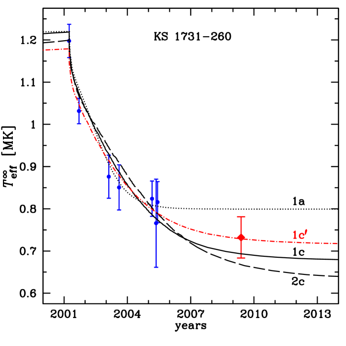
Fig. 2: Theoretical cooling curves for different neutron-star models compared with observations of KS 1731–260. The observational data are from Table 1 of Ref. [131]. The blue dots correspond to the observations used in [128], and the red diamond is the new observation. The $1\sigma$-errorbars are plotted. For the cooling curves, we use the numerical data and notations from Ref. [128]: 1a – $M=1.6\,M_{\odot}$, $T_{0}=0.8$ MK, $E_{44}=2.6$; 1c – $M=1.6\,M_{\odot}$, $T_{0}=0.67$ MK, $E_{44}=2.4$; 2c – $M=1.4\,M_{\odot}$, $T_{0}=0.63$ MK, $E_{44}=2.4$. The model 1a, unlike the other three models, assumes an accreted envelope and a moderate (in terms of [128]) neutron superfluidity in the crust. The curve marked $\mathrm{1c}^{\prime}$ was not shown in [128]. It corresponds to $M=1.65\,M_{\odot}$, $T_{0}=0.7$ MK, $E_{44}=2$.

In 2008, a cooling curve of SXT MXB 1659–29 was constructed for crustal thermal-relaxation stage, which had been observed during 6 years [132]. This curve generally agreed with the theory. In 2012, however, the spectrum suddenly changed, as if the temperature abruptly dropped [133]. However, the spectral evolution driven by the cooling has already had to reach an equilibrium. The observed change of the spectrum can be explained by a change of the line-of-sight hydrogen column density. The cause of this change remains unclear. Indications to variations of $N_{\mathrm{H}}$ were also found in the cooling qLMXB EXO 0748–676 [134].

Several other qLMXBs have recently turned into quiescence and show signs of thermal relaxation of the neutron-star crust. A luminosity decline was even seen during a single 8-hour observation of SXT XTE J1709–267 after the end of the active phase of accretion [135]. Analyses of observations of some qLMXBs (XTE J1701–462 [136, 137], EXO 0748–676 [138]) confirm the conclusions of Shternin et al. [128] on the crystalline structure of the crust and give additional information on the heating and composition of the crust of accreting neutron stars [135, 139, 138]. In § 4.5 we will discuss the interpretation of the observed qLMXB spectra that underlies such analysis.

Transiently accreting X-ray pulsars Aql X-1, SAX J1808.4–3658, and IGR J00291+5734 reveal similar properties, but an analysis of their spectral evolution is strongly impeded by the possible presence of a nonthermal component and hot polar caps (see [140, 141], and references therein). Their X-ray luminosities in quiescence vary nonmonotonically, as well as those of qLMXBs Cen X-4 [142] and EXO 1745–248 [143]. The variations of thermal flux that do not conform to the thermal-relaxation scenario may be caused by an accretion on the neutron star, which slows down but does not stop in quiescence [144, 138, 141].

3.2 Radio pulsars

There are several normal pulsars whose spectra clearly reveal a thermal component: these are relatively young (of the age $t_{*}\lesssim 10^{5}$ years) pulsars J1119–6127, B1706–44, and Vela, and middle-aged ($t_{*}\sim 10^{6}$ years) pulsars B0656+14, B1055$-$52, and Geminga. The spectra of the latter three objects, dubbed “Three Musketeers” [145], are described by a three-component model, which includes a power-law spectrum of magnetospheric origin, a thermal spectrum of hot polar caps, and a thermal spectrum of the rest of the surface [116]. In most works the thermal components of pulsar spectra is interpreted with the blackbody model, and less often a model of the fully ionized H atmosphere with a predefined surface gravity. We will see that both are physically ungrounded. Only recently, in Ref. [146], the X-ray radiation of PSR J1119–6127 was interpreted using a H atmosphere model with allowance for the incomplete ionization. This result will be described in § 8.4.

A convenient characteristic of the slowdown of pulsar rotation is the loss rate of the rotational kinetic energy $\dot{E}_{\mathrm{rot}}=-I\Omega\dot{\Omega}$ of a standard rotator with the moment of inertia $I=10^{45}\mbox{~{}g~{}cm}^{2}$, typical of neutron stars, where $\Omega=2\pi/\mathcal{P}$ is the angular frequency of the rotation, and $\dot{\Omega}$ is its time derivative (see [147]). As follows from observations, spectra of millisecond pulsars with $\dot{E}_{\mathrm{rot}}>10^{35}\mbox{~{}erg~{}s}^{-1}$ are mainly nonthermal. However, millisecond pulsars PSR J0030+0451, J0437 – 4715, J1024–0719, and J2124–3358, with $\dot{E}_{\mathrm{rot}}\lesssim 10^{34}\mbox{~{}erg~{}s}^{-1}$ show a thermal spectral component on the nonthermal background. In § 4.6 we will consider interpretation of this thermal component based on photosphere models.

3.3 Bursters

Accreting neutron stars in close binary systems, which produce X-ray bursts with intervals from hours to days, are called bursters. The theory of the bursters were formulated in [148] (see also review [149]).

During intervals between the bursts, a burster’s atmosphere does not essentially differ from an atmosphere of a cooling neutron star. In such periods, the bulk of the observed X-ray radiation arises from transformation of gravitational energy of the accreting matter into thermal energy. The matter, mostly consisting of hydrogen and helium, piles up on the surface and sooner or later (usually during several hours or days) reaches such densities and temperatures that a thermonuclear burst is triggered, which is observed from the Earth as a Type I X-ray burst. Some of such bursts last over a minute and are called long X-ray bursts. They arise in the periods when the accretion rate is not high, so that the luminosity $L_{\mathrm{ph}}$ before the burst does not exceed several percent of the Eddington limit $L_{\mathrm{Edd}}$ (§ 4.2). In this case, the inner part of the accretion disk is a hot ($k_{\mathrm{B}}T\sim 20-30$ keV) flow of matter with an optical thickness about unity. It almost does not affect the burst, nor screen it [151]. As we will see in § 4.3, the observed spectrum of a burster, its evolution during a long burst, and subsequent relaxation are successfully interpreted with nonmagnetic atmosphere models.

But if the accretion rate is higher, so that $L_{\mathrm{ph}}\gtrsim 0.1L_{\mathrm{Edd}}$, then the accretion disk is relatively cool and optically thick down to the neutron-star surface. In this case, the disk can strongly shield the burst and reprocess its radiation [152, 153], while at the surface a boundary spreading layer is formed. The theory of such layer is developed in [154, 155]. The spreading layer spoils the spectrum so that its usual decomposition becomes ambiguous and needs to be modified, as described in [156, 157].

3.4 Radio quiet neutron stars

The discovery of radio quiet neutron stars, whose X-ray spectra are apparently purely thermal, has become an important milestone in astrophysics. The radio quiet neutron stars include central compact objects in supernova remnants (CCOs) [160, 161] and X-ray dim isolated neutron stars (XDINSs) [162, 39, 40, 163, 161].

Exactly seven XDINSs are known since 2001, and they are dubbed “Magnificent Seven” [39]. Observations have provided stringent upper limits ($\lesssim 0.1$ mJy) to their radio emission [165]. XDINSs have longer periods ($>3$ s) than the majority of pulsars, and their magnetic field estimations by Eq. (1) give, as a rule, rather high values $B\sim(10^{13}$ – $10^{14})$ G [40, 164]. It is possible that XDINSs are descendant of magnetars [40, 41, 163].

About ten CCOs are known to date [166, 161]. Pulsations have been found in radiation of three of them. The periods of these pulsations are rather small (0.1 s to 0.42 s) and very stable. This indicates that CCOs have relatively weak magnetic field $B\sim 10^{11}$ G, at contrast to XDINSs. For this reason they are sometimes called “antimagnetars” [166, 161, 167]. Large amplitudes of the pulsations of some CCOs indicate strongly nonuniform surface temperature distribution. To explain it, some authors hypothesized that a superstrong magnetic field might be hidden in the neutron-star crust [168].

The X-ray source 1RXS J141256.0+792204, which was discovered in 2008 and dubbed Calvera, initially was considered as a possible eighth object with the properties of the “Magnificent Seven” [169]. However, subsequent observations suggest that its properties are closer to the CCOs. In 2013, observations of Calvera at the orbital observatory Chandra provided the period derivative $\dot{\mathcal{P}}$ [170]. According to Eq. (1), its value corresponds to $B\approx 4.4\times 10^{11}$ G. The authors [170] characterize Calvera as an “orphaned CCO,” whose magnetic field is emerging through supernova debris. Calvera is also unique in that it is the only energetic pulsar that emits virtually no radio nor gamma radiation, which places constraints on models for particle acceleration in magnetospheres [170].

3.5 Neutron stars with absorption lines in their thermal spectra

CCO 1E 1207.4–5209 has been the first neutron star whose thermal spectrum was found to possess features resembling two broad absorption lines [171]. The third and fourth spectral lines were reported [172], but their statistical significance was called in question [173]. It is possible that the complex shape of CCO PSR J0821–4300 may also be due to an absorption line [167].

Features, which are possibly related to resonant absorption, are also found in spectra of four XDINSs: RX J0720.4–3125 [174, 175], RX J1308.6+2127 (RBS1223) [176], 1RXS J$214303.7+065419$ (RBS1774) [177, 178, 179] and RX J1605.3+3249 [180]. Possible absorption features were also reported in spectra of two more XDINSs, RX J0806.4–4123 and RX J0420.0–5022 [181], but a confident identification is hampered by uncertainties related to ambiguous spectral background subtraction [164]. Only the “Walter star” RX J1856.5 – 3754 that was discovered the first of the “Magnificent Seven” [182] has a smooth spectrum without any features in the X-ray range [183].

An absorption line has been recently found in the spectrum of SGR 0418+5729 [184]. Its energy varies from $<1$ keV to $\sim 4$ keV with the rotational phase. The authors interpret it as a proton cyclotron line associated with a highly nonuniform magnetic-field distribution between $\sim 2\times 10^{14}$ G and $\sim 10^{15}$ G. The discrepancy with the estimate $B\sim 6\times 10^{12}$ G according to Eq. (1) [51] the authors [184] explain by an absence of a large-scale dipolar component of the superstrong magnetic field (which can be, e.g., contained in spots). They reject the electron-cyclotron interpretation on the grounds that it would imply $B\sim(1-5)\times 10^{11}$ G, again at odds with the estimate [51]. Note that the latter contradiction can be resolved in the models [53, 54, 56, 55] that involve a residual accretion torque (§ 1). There is also no discrepancy if the line has a magnetospheric rather than photospheric origin. Similar puzzling lines had been previously observed in gamma-ray bursts of magnetars [185, 186, 48].

Unlike the radio quiet neutron stars, spectra of the ordinary pulsars were until recently successfully described by a sum of smooth thermal and nonthermal spectral models. The first exception is the radio pulsar PSR J1740+1000, in whose X-ray spectrum is found to possess absorption features [187]. This discovery fills the gap between the spectra of pulsars and radio quiet neutron stars and shows that similar spectral features can be pertinent to different neutron-star classes.

Currently there is no unambiguous and incontestable theoretical interpretation of the features in neutron-star spectra. There were more or less successful attempts to interpret spectra of some of them. In § 8 we will consider the interpretations that are based on magnetic neutron-star atmosphere models.

4 Nonmagnetic atmospheres

4.1 Which atmosphere can be treated as nonmagnetic?

The main results of atmosphere modeling are the outgoing radiation spectra. Zavlin et al. [188] formulated the conditions that allow calculation of a neutron-star spectrum without account of the magnetic field. In the theory of stellar atmospheres, interaction of electromagnetic radiation with matter is conventionally described with the use of opacities $\varkappa$, that is absorption and scattering cross sections counted per unit mass of the medium. Opacities of fully ionized atmospheres do not depend on magnetic field at the frequencies $\omega$ that are much larger than the electron cyclotron frequency $\omega_{\mathrm{c}}$, which corresponds to the energy $\hbar\omega_{\mathrm{c}}\approx 11.577\,B_{12}\mbox{~{}keV}.$ On this ground, Zavlin et al. [188] concluded that for the energies $\hbar\omega\sim(1$ – 10) $k_{\mathrm{B}}T$ that correspond to the maximum of a thermal spectrum one can neglect the magnetic-field effects on opacities, if

$$B\ll(m_{\mathrm{e}}c/\hbar e)\,k_{\mathrm{B}}T\sim 10^{10}\,T_{6}\mbox{~{}G}.$$ (24)

Strictly speaking, the estimate (24) is very relative. If the atmosphere contains an appreciable fraction of atoms or ions in bound states, then even a weak magnetic field changes the opacities by spectral line splitting (the Zeeman and Paschen-Back effects). Besides, magnetic field polarizes radiation in plasmas [189]. The Faraday and Hanle effects that are related to the polarization serve as useful tools for studies of the stellar atmospheres and magnetic fields, especially the Sun (see [190], for a review). But the bulk of neutron-star thermal radiation is emitted in X-rays, whose polarimetry only begins to develop, therefore one usually neglects such fine effects for the neutron stars.

Magnetic field drastically affects opacities of partially ionized photospheres, if the electron cyclotron frequency $\hbar\omega_{\mathrm{c}}$ is comparable to or larger than the electron binding energies $E_{\mathrm{b}}$. Because of the high density of neutron-star photospheres, highly excited states do not survive as they have relatively large sizes and low binding energies (the disappearance of bound states with increasing density is called pressure ionization). For low-lying electron levels of atoms and positive atomic ions in the absence of a strong magnetic field, the binding energy can be estimated as $E_{\mathrm{b}}\sim(Z+1)^{2}$ Ry, where $Z$ is the charge of the ion, and $\mbox{Ry}=m_{\mathrm{e}}e^{4}/(2\hbar^{2})=13.6057$ eV is the Rydberg constant in energy units. Consequently the condition $\hbar\omega_{\mathrm{c}}\ll E_{\mathrm{b}}$ is fulfilled at

$$B\ll B_{0}\,(Z+1)^{2}/2,$$ (25)

where

$$B_{0}=\frac{m_{\mathrm{e}}^{2}\,c\,e^{3}}{\hbar^{3}}=2.3505\times 10^{9}\mbox{~{}G}$$ (26)

is the atomic unit of magnetic field. The conditions (24) and (25) are fulfilled for most millisecond pulsars and accreting neutron stars.

4.2 Radiative transfer

A nonmagnetic photosphere of a neutron star does not essentially differ from photospheres of the ordinary stars. However, quantitative differences can give rise to specific problems: for instance, the strong gravity results in high density, therefore the plasma nonideality that is usually neglected in stellar atmospheres can become significant. Nevertheless, the spectrum that is formed in a nonmagnetic neutron-star photosphere can be calculated using the conventional methods that are described in the classical monograph by Mihalas [104]. For stationary neutron-star atmospheres, thanks to their small thickness, the approximation of plane-parallel locally uniform layer is quite accurate. The local uniformity means that the specific intensity at a given point of the surface can be calculated neglecting the nonuniformity of the flux distribution over the surface, that is, the nonuniformity of $T_{\mathrm{s}}$.

Almost all models of neutron-star photospheres assume the radiative and local thermodynamic equilibrium (LTE; see [191] for a discussion of this and alternative approximations). Under these conditions, it is sufficient to solve a system of three basic equations: equations of radiative transfer, hydrostatic equilibrium, and energy balance.

The first equation can be written in a plane-parallel layer as (see, e.g., [192])

$$\cos\theta_{k}\frac{\mathrm{d}I_{\omega}(\hat{\mathbf{k}})}{\mathrm{d}y_{\mathrm{col}}}=\varkappa_{\omega}I_{\omega}-\int_{(4\pi)}\!\!\varkappa_{\omega}^{\mathrm{s}}(\hat{\mathbf{k}}^{\prime},\hat{\mathbf{k}})I_{\omega}(\hat{\mathbf{k}}^{\prime})\mathrm{d}\hat{\mathbf{k}}^{\prime}-\varkappa_{\omega}^{\mathrm{a}}\mathcal{B}_{\omega,T},$$ (27)

where $\hat{\mathbf{k}}$ is the unit vector along $\bm{k}$, $\varkappa_{\omega}=\varkappa_{\omega}^{\mathrm{a}}+\int_{(4\pi)}\varkappa_{\omega}^{\mathrm{s}}(\hat{\mathbf{k}}^{\prime},\hat{\mathbf{k}})\,\mathrm{d}\hat{\mathbf{k}}^{\prime}/(4\pi)$ is the total opacity, $\varkappa_{\omega}^{\mathrm{a}}$ and $\varkappa_{\omega}^{\mathrm{s}}(\hat{\mathbf{k}}^{\prime},\hat{\mathbf{k}})$ are its components due to, respectively, the true absorption and the scattering that changes the ray direction from $\hat{\mathbf{k}}^{\prime}$ to $\hat{\mathbf{k}}$, and $\mathrm{d}\hat{\mathbf{k}}^{\prime}=\sin\theta_{k^{\prime}}\mathrm{d}\theta_{k^{\prime}}\mathrm{d}\varphi_{k^{\prime}}$ is a solid angle element. Most studies of the neutron-star photospheres neglect the dependence of $\varkappa_{\omega}^{\mathrm{s}}$ on $\hat{\mathbf{k}}^{\prime}$ and $\hat{\mathbf{k}}$. As shown in [193], the inaccuracy that is introduced by this simplification does not exceed 0.3% for the thermal spectral flux of a neutron star at $\hbar\omega<1$ keV and reaches a few percent at higher energies.

For simplicity, in Eq. (27) we have neglected polarization of radiation and a change of frequency at the scattering. In general, the radiative transfer equation includes an integral of $I_{\omega}$ not only over angles, but also over frequencies, and contains, with account of polarization, a vector of Stokes parameters instead of $I_{\omega}$, while the scattering cross section is replaced by a matrix. A detailed derivation of the transfer equations for polarized radiation is given, e.g., in [192], and solutions of the radiative transfer equation with frequency redistribution are studied in [191].

The condition of hydrostatic equilibrium follows from Eq. (5). Given that $|R-r|\ll R$, $|M-M_{r}|\ll M$, and $P\ll\rho c^{2}$ in the photosphere, we have

$$\frac{\mathrm{d}P}{\mathrm{d}y_{\mathrm{col}}}=g-g_{\mathrm{rad}},$$ (28)

where (see, e.g., [194])

$$g_{\mathrm{rad}} = \frac{1}{c}\,\frac{\mathrm{d}}{\mathrm{d}y_{\mathrm{col}}}\int_{0}^{\infty}\mathrm{d}\omega\int_{(4\pi)}\mathrm{d}\hat{\mathbf{k}}\,\cos^{2}\theta_{k}\,I_{\omega}(\hat{\mathbf{k}})$$ (29)

$$\approx \frac{2\pi}{c}\int_{0}^{\infty}\mathrm{d}\omega\,\varkappa_{\omega}\int_{0}^{\pi}\cos\theta_{k}\,I_{\omega}(\hat{\mathbf{k}})\sin\theta_{k}\,\mathrm{d}\theta_{k}.\hskip 20.00003pt$$

The last approximate equality becomes exact for the isotropic scattering. The quantity $g_{\mathrm{rad}}$ takes account of the radiation pressure that counteracts gravity. It becomes appreciable at $T_{\mathrm{eff}}\gtrsim 10^{7}$ K. Therefore, $g_{\mathrm{rad}}$ is usually dropped in calculations of the spectra of the cooler isolated neutron stars, but included in the models of relatively hot bursters. Radiative flux of the bursters amply increases during the bursts, thus increasing $g_{\mathrm{rad}}$. The critical value of $g_{\mathrm{rad}}$ corresponds to the limit of stability, beyond which matter inevitably flows away under the pressure of light. In a hot nonmagnetic atmosphere, where the Thomson scattering dominate, the instability appears when the luminosity $L_{\mathrm{ph}}$ exceeds the Eddington limit

$$L_{\mathrm{Edd}} = 4\pi c\,(1+z_{g})\,{GMm_{\mathrm{p}}}/{\sigma_{\mathrm{T}}}$$ (30)

$$\approx 1.26\times 10^{38}\,(1+z_{g})\,({M}/{M_{\odot}})~{}~{}\textrm{erg~{}s}^{-1},$$

where $m_{\mathrm{p}}$ is the proton mass, and

$$\sigma_{\mathrm{T}}=\frac{8\pi}{3}\left(\frac{e^{2}}{m_{\mathrm{e}}c^{2}}\right)^{2}$$ (31)

is the Thomson cross section, A temperature-dependent relativistic correction to $\sigma_{\mathrm{T}}$ [195] increases $L_{\mathrm{Edd}}$ approximately by 7% at typical temperatures $\sim 3\times 10^{7}$ K at the bursters luminosity maximum [151, 194].

Finally, the energy balance equation in the stationary state expresses the fact that the energy acquired by an elementary volume equals the lost energy. The radiative equilibrium assumes that the energy transport through the photosphere is purely radiative, that is, one neglects electron heat conduction and convection, as well as other sources and leaks of heat. Under these conditions, the energy balance equation reduces to

$$\int_{0}^{\infty}\mathrm{d}\omega\int_{(4\pi)}I_{\omega}(\hat{\mathbf{k}})\,\cos\theta_{k}\,\mathrm{d}\hat{\mathbf{k}}=F_{\mathrm{ph}},$$ (32)

where $F_{\mathrm{ph}}$ is the local flux at the surface that is related to $T_{\mathrm{s}}$ according to Eq. (11).

Radiation is almost isotropic at large optical depth

$$\tau_{\omega}=\int_{r}^{\infty}\varkappa_{\omega}(r^{\prime})\,\mathrm{d}y_{\mathrm{col}}(r^{\prime}),$$ (33)

therefore one may restrict to the first two terms of the intensity expansion in spherical functions:

$$I_{\omega}(\hat{\mathbf{k}})=J_{\omega}+\frac{3}{4\pi}\bm{F}_{\omega}\cdot\hat{\mathbf{k}}.$$ (34)

Here, $J_{\omega}=\frac{1}{4\pi}\int_{(4\pi)}I_{\omega}(\hat{\mathbf{k}})\,\mathrm{d}\hat{\mathbf{k}}$ is the mean intensity, averaged over all directions, and $\bm{F}_{\omega}=\int_{(4\pi)}I_{\omega}(\hat{\mathbf{k}})\hat{\mathbf{k}}\,\mathrm{d}\hat{\mathbf{k}}$ is the diffusive flux vector. Then integro-differential equation (27) reduces to a diffusion-type equation for $J_{\omega}$. If scattering is isotropic, then in the plane-parallel locally-uniform approximation the stationary diffusion equation has the form

$$\frac{\mathrm{d}^{2}}{\mathrm{d}\tau_{\omega}^{2}}\,\frac{J_{\omega}}{3}=\frac{\varkappa_{\omega}^{\mathrm{s}}}{\varkappa_{\omega}}\,(J_{\omega}-\mathcal{B}_{\omega,T})$$ (35)

(see [196] for derivation of the diffusion equation from the radiative transfer equation in a more general case). Sometimes the diffusion approximation is applied to the entire atmosphere, rather than only to its deep layers. In this case, one has to replace $J_{\omega}/3$ on the left-hand side of Eq. (35) by $f_{\omega}J_{\omega}$, where $f_{\omega}(\tau_{\omega})$ is the so called Eddington factor [104], which is determined by iterations of the radiative-transfer and energy-balance equations with account of the boundary conditions (see [188] for details).

In modeling bursters atmospheres, one usually employs Eq. (35) with the Eddington factor on the left-hand side and an additional term on the right-hand side, a differential Kompaneets operator [197] acting on $J_{\omega}$ (see, e.g., [198, 199, 200, 201]). The Kompaneets operator describes, in the diffusion approximation, the photon frequency redistribution due to the Compton effect, which cannot be neglected at the high temperatures typical of the bursters.

In order to close the system of equations of radiative transfer and hydrostatic balance, one needs the EOS and opacities $\varkappa_{\omega}^{\mathrm{s,a}}$ for all densities and temperatures encountered in the photosphere. In turn, in order to determine the EOS and opacities, it is necessary to find ionization distribution for the chemical elements that compose the photosphere. The basis for solution of these problems is provided by quantum mechanics of all particle types that give a significant contribution to the EOS or opacities. In the nonmagnetic neutron-star photospheres, these particles are only the electrons and atomic ions, because molecules do not survive the typical temperatures $T\gtrsim 3\times 10^{5}$ K.

We will not consider in detail the calculations of the EOS and opacities in the absence of a strong magnetic field, because they do not basically differ from the ones for the ordinary stellar atmospheres, which have been thoroughly considered, e.g., in the review [202]. Detailed databases have been developed for them (see [203], for review), the most suitable of which for the neutron-star photospheres are OPAL [204] and OP [205]. In the particular cases where the neutron-star atmosphere consists of hydrogen or helium, all binding energies are smaller than $k_{\mathrm{B}}T$, therefore the approximation of an ideal gas of electrons and atomic nuclei is applicable.

Systematic studies of neutron-star photospheres of different chemical compositions, from hydrogen to iron, started from the work by Romani [207]. In the subsequent quarter of century, the nonmagnetic neutron-star photospheres have been studied in many works (see [116] for a review). Databases of neutron-star hydrogen photosphere model spectra have been published [188, 208, 209], and a numerical code for their calculation has been released [193]. A publicly available database of model spectra for the carbon photospheres has been recently published [211]. In addition, model spectra were calculated for neutron-star photospheres composed of helium, nitrogen, oxygen, iron (e.g., [212, 213, 209, 214]), and mixtures of different elements [208, 213].

4.3 Atmospheres of bursters

Burster spectra were calculated by many authors (see, e.g., [151], for references), starting from the pioneering works [215, 216, 153] (see, e.g., [151], for references). These calculations as well as observations show that the X-ray spectra of bursters at high luminosities are close to so called diluted blackbody spectrum

$$F_{\omega}\approx w\mathcal{B}_{\omega,T_{\mathrm{bb}}},$$ (36)

where $\mathcal{B}_{\omega,T}$ is the Planck function (18), the parameter $T_{\mathrm{bb}}$ is called color temperature, normalization $w$ is a dilution factor, and the ratio $f_{\mathrm{c}}=T_{\mathrm{bb}}/T_{\mathrm{eff}}$ (typically $\sim 3/2$) is called color correction [217, 216, 151]. The apparent color temperature $T_{\mathrm{bb}}^{\infty}$ is related to $T_{\mathrm{bb}}$ by the relation analogous to (6).

If the luminosity reaches the Eddington limit during a thermonuclear burst, then the photosphere radius $R_{\mathrm{ph}}$ first increases, and goes back to the initial value $R$ at the relaxation stage [195]. Based on this model, Kaminker et al. [218] suggested a method of analysis of the Eddington bursts of the bursters and for the first time applied it to obtaining constraints of the parameters of the burster MXB 1728–34. Subsequently this method was amended and modernized by other authors (see [151], for references).

According to Eq. (9), the bolometric flux equals $F_{\mathrm{bol}}=L_{\mathrm{ph}}^{\infty}/(4\pi D^{2})=\sigma_{\mathrm{SB}}(T_{\mathrm{eff}}^{\infty})^{4}(R_{\mathrm{ph}}^{\infty}/D)^{2}$. But the approximation (36) implies $F_{\mathrm{bol}}=w\sigma_{\mathrm{SB}}(T_{\mathrm{bb}}^{\infty})^{4}(R_{\mathrm{ph}}^{\infty}/D)^{2}$. Therefore, at the late stage of a long burst, when $R_{\mathrm{ph}}=R={}$constant, $w\propto f_{\mathrm{c}}^{-4}$. On the other hand, the dependence of $f_{\mathrm{c}}$ on $L_{\mathrm{ph}}$ can be obtained from numerical calculations. This possibility lies in the basis of the method of studying bursters that was implemented in the series of papers by Suleimanov et al. [200, 151]. The calculations show that $f_{\mathrm{c}}$ mainly depends on the ratio $l_{\mathrm{ph}}=L_{\mathrm{ph}}/L_{\mathrm{Edd}}$, and also on gravity $g$ and chemical composition of the photosphere (mostly on the helium-to-hydrogen fractional abundance, and to a less extent on the content of heavier elements). Having approximated the observed spectral normalizations $f_{\mathrm{c}}^{-4}(l_{\mathrm{ph}})$ by the results of theoretical calculations, one finds the chemical composition that provides an agreement of the theory with observations. For this selected composition, one finds the color correction that corresponds to the observed one at different values of $g$, and thus obtains a curve of allowable values in the $(M,R)$-plane. The point at this curve that satisfies the condition $F_{\mathrm{bol}}=l_{\mathrm{ph}}F_{\mathrm{Edd}}$, $F_{\mathrm{Edd}}=L_{\mathrm{Edd}}/[4\pi D^{2}(1+z_{g})^{2}]$ being the bolometric flux that corresponds to the Eddington luminosity Eq. (30), gives an estimate of the mass and radius of the neutron star, if the distance $D$ is known. If $D$ is unknown, then this analysis allows one to obtain restrictions on joint values of $M$, $R$, and $D$.

This method was successfully applied to analyzing the long bursts of bursters 4U 1724–307 [151] and GS 1826–24 [219]. In both cases, there was a marked agreement of the observed and calculated dependences $f_{\mathrm{c}}(l_{\mathrm{ph}})$. In [219], the authors have also simulated the light curves, that is, the time dependences of $F_{\mathrm{bol}}$. As well as in an earlier work [220], they managed to find the chemical composition of the atmosphere and the accretion rate that give an agreement of the theoretical light curve of each burst and of the intervals between the bursts with observations. Thus they obtained an absolute calibration of the luminosity. A comparison of the theoretical and observed dependences gives an estimate of the ratio $f_{\mathrm{c}}/(1+z_{g})$, which does not depend on the distance $D$, thus providing additional constraints to the neutron-star mass and radius [151, 219]. A possible anisotropy of the emission, which modifies the total flux (e.g., because of screening and reflection of a part of radiation by an accretion disk) is equivalent to a multiplication of $D$ by a constant factor, therefore it does not affect the $D$-independent estimates [219].

In [221, 222, 223] the authors used a simplified analysis of spectra of bursters, ignoring the dependence $f_{\mathrm{c}}(l_{\mathrm{ph}})$, but only assuming that the Eddington luminosity is reached at the “touchdown point,” determined by the maximum of the color temperature. This assumption is inaccurate, therefore such simplified analysis fails: it gives considerably lower $R$ values, than the method described above. In addition, the authors of [221, 222, 223] analyzed the “short” bursts, for which the theory fails to describe the dependence $f_{\mathrm{c}}(l_{\mathrm{ph}})$, and the usual separation of spectral components becomes ambiguous (see § 3.3). Therefore, the simplified estimates of neutron-star parameters [221, 222, 223] are unreliable (see the discussion in [151]).

We must note that the current results for the bursters still do leave some open questions. First, the estimates for two different sources in [151] and [219] are hard to conciliate: in the case of the H atmosphere model, the former estimate indicates a relatively large neutron-star radius, thus a stiff EOS, whereas the latter gives a constraint, which implies a soft EOS. Second, a good agreement between the theory and observations has been achieved only for a restricted decaying part of the lightcurves. Third, there is a lack of explanation to different normalizations of spectra for the bursts that have different recurrence times. In [219], the authors discuss these uncertainties and possible prospects of their resolution with the aid of future observations.

4.4 Photospheres of isolated neutron stars

Nonmagnetic atmospheres of isolated neutron stars differ from accreting neutron stars atmospheres, first of all, by a lower effective temperature $T_{\mathrm{s}}\sim 3\times(10^{5}$ – $10^{6}$) K, and may be also by chemical composition. Examples of spectra of such atmospheres are given in Fig. 3.

If there was absolutely no accretion on a neutron star, then the atmosphere should consist of iron. A spectrum of such atmosphere has the maximum in the same wavelength range as the blackbody spectrum, but contains many features caused by bound-bound transitions and photoionization [207, 212, 224, 208]. Absorption lines and photoionization edges are smeared with increasing $g$, because the photosphere becomes denser, thus increasing the effects leading to line broadening [225] (for example, fluctuating microfields in the plasma [226]).

If the atmosphere consists of hydrogen and helium, the spectrum is smooth, but shifted to higher energies compared to the blackbody spectrum at the same effective temperature [207, 188]. As shown by Zavlin et al. [188], this shift is caused by the decrease of light-element opacities according to the law $\varkappa_{\omega}\propto\omega^{-3}$ at $\hbar\omega>k_{\mathrm{B}}T\sim 0.1$ keV, which makes photons with larger energies to come from deeper and hotter photosphere layers. Zavlin et al. [188] payed attention also to the polar diagrams of radiation coming from the atmosphere. Unlike the blackbody radiation, it is strongly anisotropic ($I_{\omega}(\hat{\mathbf{k}})$ quickly decreases at large angles $\theta_{k}$), and the shape of the polar diagram depends on the frequency $\omega$ and on the chemical composition of the atmosphere.

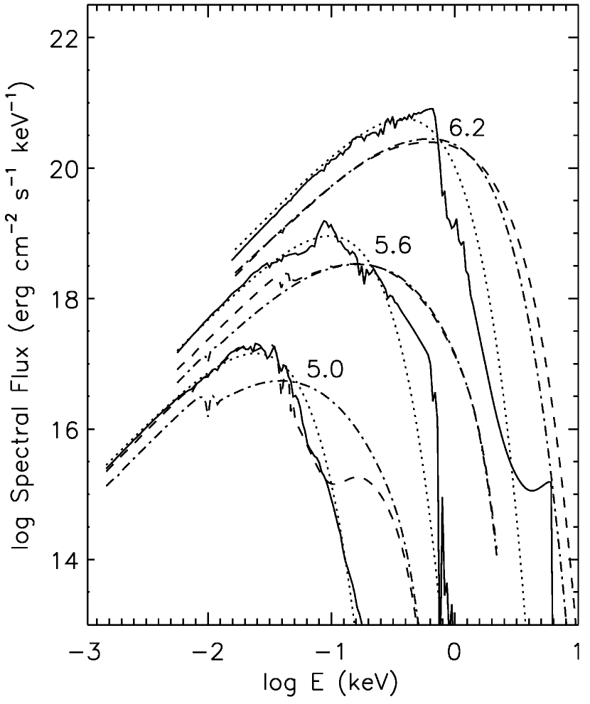
Fig. 3: Radiation energy flux densities as functions of photon energy $E=\hbar\omega$ for a photosphere composed of iron (solid lines), helium (dashed lines), and hydrogen (dot-dashed lines) as compared to the blackbody spectrum (dotted curves) at $g_{14}=2.43$ for different values of effective temperature (numbers at the curves correspond to $\log\,T_{\mathrm{eff}}$ [K]). (Fig. 3 from [213], courtesy of J. Pons and ©AAS.)

Suleimanov & Werner [227] have taken account of the Compton effect on the spectra of isolated neutron stars, using the same technique as for the bursters. They have shown that this effect results in a decrease of the high-energy flux at $\hbar\omega\gg 1$ keV for the hydrogen and helium atmospheres. It becomes considerable at high effective temperatures $T_{\mathrm{s}}>10^{6}$ K, where the spectral maximum shifts to the energies $E\gtrsim 1$ keV. This effect makes the spectra of hot hydrogen and helium atmospheres closer to the blackbody spectrum with color correction $f_{\mathrm{c}}\approx 1.6$ – 1.9.

Papers [224, 228] stand apart, being the only ones where non-LTE calculations were done for a spectrum of an iron neutron-star atmosphere. At $T=2\times 10^{5}$ K, the difference from the LTE model is about 10% for the flux in the lines and much less in the continuum [224, 208]. As noted in [208], the difference may be larger at higher temperatures, which turned out to be the case indeed in [228].

Pons et al. [213] performed a thorough study in attempt to describe the observed spectrum of the Walter star RX J1856.5 – 3754 by the nonmagnetic atmosphere models with various chemical compositions. It turned out that the hydrogen atmosphere model that reproduces the X-ray part of the spectrum predicts approximately 30 times larger optical luminosity than observed, whereas an iron-atmosphere model corresponds to a too small radius. This demonstrates once again that a neutron-star radius estimate strongly depends on the assumptions on its atmosphere. Satisfactory results have been obtained for a chemical composition corresponding to the ashes of thermonuclear burning of matter that was accreted on the star at the early stage of its life. This model, as well as other models of atmospheres composed of elements heavier than helium, predicted absorption lines in the X-ray spectrum. However, subsequent deep X-ray observations with space observatories Chandra [229] and XMM-Newton [83] have not found such lines.

The failure of the interpretation of the Walter star spectrum with nonmagnetic atmosphere models can be explained by the presence of a strong magnetic field. The field is indicated by a nearby nebula glowing in the H$\alpha$ line [230]. Such nebulae are found near pulsars, which ionize interstellar hydrogen by shock waves arising from hypersonic pulsar magnetosphere interaction with interstellar medium [52, 231]. Doubts had initially been cast on the pulsar analogy by the absence of observed pulsations of radiation of this star, but soon such pulsations were discovered [232]. Interpretation of the Walter star spectrum with magnetic atmosphere models will be considered in § 8.1.

The first successful interpretation of an isolated neutron star spectrum based on a nonmagnetic atmosphere model was done in [214]. The authors showed that the observed X-ray spectrum of the CCO in Cassiopeia A supernova remnant, which appeared around 1680, is well described by a carbon atmosphere model with the effective temperature $T_{\mathrm{eff}}\sim 2\times 10^{6}$ K. Subsequent observations revealed that $T_{\mathrm{eff}}$ appreciably decreases with time [233], which was explained by the heat-carrying neutrino emission outburst caused by the superfluid transition of neutrons [234, 235]. At $t_{*}\approx 330$ yrs this agrees with the cooling theory [97]. An independent analysis [236] confirmed the decrease of the registered flux, but the authors stressed that the statistical significance of this result is not high and that the same observational data allow other interpretations. Recently, a spectrum of one more CCO, residing in supernova remnant HESS J1731–347, was also satisfactorily described by a nonmagnetic carbon atmosphere model [237].

4.5 Atmospheres of neutron stars in qLMXBs

Many SXTs reside in globular clusters, whose distances are known with accuracies of 5 – 10%. This reduces a major uncertainty that hampers the spectral analysis. As we noted in § 3, spectra of SXTs in quiescence, called qLMXBs, are probably determined by neutron-star thermal emission. In early works, these spectra were interpreted with the Planck function, which overestimated the effective temperature and underestimated the effective radius of emitting area. However, Rutledge et al. [238, 144, 239] found that the nonmagnetic hydrogen atmosphere model provides an explanation to the SXT spectra as caused by radiation from the entire neutron-star surface with acceptable values of the temperature and radius.

Currently tens qLMXBs in globular clusters are known (they are listed in [240, 241]), and the use of hydrogen atmosphere models for their spectral analysis has become customary. For instance, the analysis of the cooling of KS 1731–260 and the other similar objects that was discussed in § 3.1 was based on the measurements of the effective temperature $T_{\mathrm{eff}}$ with the use of the models [188] and NSATMOS [209].

In many works (including [130, 132, 131]), the neutron-star mass and radius were a priori fixed to $M=1.4\,M_{\odot}$ and $R=10$ km, which entrain $g_{14}=2.43$. It was shown in [209], that such fixing of $g$ may strongly bias estimates of the neutron-star parameters (which means, in particular, that the estimates of $T_{\mathrm{eff}}$ for KS 1731–260 and MXB 1659–29, quoted in § 3.1, are unreliable). An analysis of thermal spectrum of qLMXB X7 in the globular cluster 47 Tuc, free of such fixing, gave a 90%-confidence area of $M$ and $R$ estimates, which agrees with relatively stiff EOSs of supranuclear matter [209]. However, the estimates that were obtained in [242] by an analogous analysis for five qLMXBs in globular clusters, although widely scattered, generally better agree with soft EOSs. In [243, 244], thermal spectra of two qLMXBs were analyzed using hydrogen and helium atmosphere models. It turned out that the former model leads to low estimates of $M$ and $R$, compatible with the soft EOSs, while the latter yields high values, which require a stiff EOS of superdense matter. Thus, despite the progress achieved in recent years, the estimates of neutron-star masses and radii based on the qLMXBs spectral analysis are not yet definitive.

4.6 Photospheres of millisecond pulsars

Magnetic fields of most millisecond pulsars satisfy the weak-field criteria formulated in § 4.1. Nevertheless, magnetic field does play certain role, because the open field line areas (“polar caps”) may be heated by deceleration of fast particles (see § 2.6). Therefore, one should take nonuniform temperature distribution into account, while calculating the integral spectrum.

Models of rotating neutron stars with hot spots were presented in many publications (e.g., [72, 245, 246], and references therein), however most of them used the blackbody radiation model. This model is acceptable for a preliminary qualitative description of the spectra and light curves of the millisecond pulsars, but a detailed quantitative analysis must take the photosphere into account. Let us consider results of such analyses.

The nearest and the brightest of the four millisecond pulsars with observed thermal radiation is PSR J0437 – 4715. It belongs to a binary system with a 6-billion-year-old white dwarf. The low effective temperature of the white dwarf ($\sim 4000$ K), as well as the brightness of the pulsar and a relatively low intensity of its nonthermal emission favor the analysis of the thermal spectrum. Recently, the pulsar’s thermal radiation has been extracted from the white-dwarf radiation even in the ultraviolet range [247], although the maximum of the pulsar thermal radiation lies at X-rays. Zavlin & Pavlov [248] showed that the thermal X-ray spectrum of PSR J0437 – 4715 can be explained by emission of two hot polar caps with hydrogen photospheres and a nonuniform temperature distribution, which was presented by the authors as a steplike function with a higher value $T\approx(1$ – $2)\times 10^{6}$ K in the central circle of radius $0.2$ – $0.4$ km and a lower value $T\approx(3$ – $5)\times 10^{5}$ K in the surrounding broad ring of radius about several kilometers.

Subsequent observations of the binary system J0437 – 4715 in spectral ranges from infrared to hard X-rays and their analysis in [249, 102, 250] have generally confirmed the qualitative conclusions of [248]. In particular, Bogdanov et al. [102, 250] reproduced not only the spectrum, but also the light curve of this pulsar at X-rays, using the model of a hydrogen atmosphere with a steplike temperature distribution, supplemented with a power-law component. These authors have also explained [251] the power-law spectral component by the Compton scattering of thermal polar-cap photons on energetic electrons in the magnetosphere or in the pulsar wind. Thus all the spectral components may have thermal origin. Finally, Bogdanov [252] reanalyzed the phase-resolved X-ray spectrum of PSR J0437 – 4715 using the value $M=(1.76\pm 0.20)\,M_{\odot}$ obtained from radio observations [253], the distance of 156.3 pc measured by radio parallax [254], a nonmagnetic hydrogen atmosphere model NSATMOS [209], and a three-level distribution of $T_{\mathrm{eff}}$ around the polar caps. As a result, he came to the conclusion that the radius of a neutron star of such mass cannot be smaller than 11 km, which favors the stiff equations of state of supranuclear matter.

The presence of a hydrogen atmosphere helps one to explain not only the spectrum but also the relatively large pulsed fraction (30 – 50%) in thermal radiation of this and the three other millisecond pulsars with observed thermal components of radiation (PSR J0030+0451, J2124–3358, and J1024–0719). According to [250, 116], such strong pulsations may indicate that all similar pulsars have hydrogen atmospheres. The measured spectra and light curves of all the four pulsars agree with this assumption [250].

5 Matter in strong magnetic fields

The conditions of § 4.1 are not satisfied for most of the known isolated neutron stars, therefore magnetic fields drastically affect radiative transfer in their atmospheres. Before going on to magnetized atmosphere models, it is useful to consider the magnetic-field effects on their constituent matter.

5.1 Landau quantization

Motion of charged particles in a magnetic field is quantized in Landau levels [255]. It means that only longitudinal (parallel to $\bm{B}$) momentum of the particle can change continuously. Motion of a classical charged particle across magnetic field is restricted to circular orbits, corresponding to a set of discrete quantum states, analogous to the states of a two-dimensional oscillator.

The complete theoretical description of the quantum mechanics of free electrons in a magnetic field is given in monograph [256]. It is convenient to characterize magnetic field by its strength in relativistic units, $b$, and in atomic units, $\gamma$:

$$b = {\hbar\omega_{\mathrm{c}}}/({m_{\mathrm{e}}c^{2}})=B/B_{\mathrm{QED}}={B_{12}}/{44.14}\,,$$ (37)

$$\gamma = B/B_{0}=425.44\,B_{12}.$$ (38)

We have already dealt with the atomic unit $B_{0}$ in § 4.1. The relativistic unit $B_{\mathrm{QED}}=m_{\mathrm{e}}^{2}c^{3}/(e\hbar)=B_{0}/\alpha_{\mathrm{f}}^{2}$ is the critical (Schwinger) field, above which specific QED effects become pronounced. In astrophysics, the magnetic field is called strong, if $\gamma\gg 1$, and superstrong, if $b\gtrsim 1$.

In the nonrelativistic theory, the distance between Landau levels equals the cyclotron energy $\hbar\omega_{\mathrm{c}}$. In the relativistic theory, Landau level energies equal $E_{N}=m_{\mathrm{e}}c^{2}\,(\sqrt{1+2bN}-1)$ ($N=0,1,2,\ldots$). The wave functions that describe an electron in a magnetic field have a characteristic transverse scale $\sim a_{\mathrm{m}}=(\hbar c/eB)^{1/2}=a_{\mathrm{B}}/\sqrt{\gamma}$, where $a_{\mathrm{B}}$ is the Bohr radius. The momentum projection on the magnetic field remains a good quantum number, therefore we have the Maxwell distribution for longitudinal momenta at thermodynamic equilibrium. For transverse motion, however, we have the discrete Boltzmann distribution over $N$.

In practice, the Landau quantization becomes important when the electron cyclotron energy $\hbar\omega_{\mathrm{c}}$ is at least comparable to both the electron Fermi energy $\epsilon_{\mathrm{F}}$ and the characteristic thermal energy $k_{\mathrm{B}}T$. If $\hbar\omega_{\mathrm{c}}$ is appreciably larger than both these energies, then most electrons reside on the ground Landau level in thermodynamic equilibrium, and the field is called strongly quantizing. For it to be the case, simultaneous conditions $\rho<\rho_{B}$ and $\zeta_{\mathrm{e}}\gg 1$ must be fulfilled, where

$$\rho_{B} = \frac{m_{\mathrm{i}}}{\pi^{2}\sqrt{2}\,a_{\mathrm{m}}^{3}\,Z}=7045\,\frac{A}{Z}\,B_{12}^{3/2}\text{ \mbox{g~{}cm${}^{-3}$}},$$ (39)

$$\zeta_{\mathrm{e}} = \frac{\hbar\omega_{\mathrm{c}}}{k_{\mathrm{B}}T}=134.34\,\frac{B_{12}}{T_{6}}.$$ (40)

In the neutron-star atmospheres, these conditions are satisfied, as a rule, at $B\gtrsim 10^{11}$ G. In the opposite limit $\zeta_{\mathrm{e}}\ll 1$, the Landau quantization can be neglected. Note that in the magnetospheres, which have lower densities, electrons can condensate on the lowest Landau level even at $B\sim 10^{8}$ G because of the violation of the LTE conditions (§ 5.9).

Ions in a neutron-star atmosphere can be treated as nondegenerate and nonrelativistic particles. The parameter $\zeta_{\mathrm{e}}$ is replaced for them by

$$\zeta_{\mathrm{i}}=\hbar\omega_{\mathrm{ci}}/k_{\mathrm{B}}T=0.0737\,(Z/A)B_{12}/T_{6}.$$ (41)

Here, $\omega_{\mathrm{ci}}=ZeB/(m_{\mathrm{i}}c)$ is the ion cyclotron frequency, and $\hbar\omega_{\mathrm{ci}}=6.35(Z/A)B_{12}$ eV is the ion cyclotron energy. In magnetar atmospheres, where $B_{12}\gtrsim 100$ and $T_{6}\lesssim 10$, the parameter $\zeta_{\mathrm{i}}$ is not small, therefore the Landau quantization of ion motion should be taken into account.

5.2 Interaction with radiation

The general expression for a differential cross section of absorption of a plane electromagnetic wave by a quantum-mechanical system can be written as (e.g., [257])

$$\mathrm{d}\sigma=\frac{4\pi^{2}}{\omega c}\left|\bm{e}\cdot\langle f|\bm{j}_{\mathrm{eff}}|i\rangle\right|^{2}\,\delta(E_{f}-E_{i}-\hbar\omega)\,\mathrm{d}\nu_{f},$$ (42)

where$|i\rangle$ and $|f\rangle$ are, respectively, the initial and final states of the system, $\mathrm{d}\nu_{f}$ is the number of final states in the considered energy interval $\mathrm{d}E_{f}$, $\bm{e}$ is the electromagnetic polarization vector, $\bm{j}_{\mathrm{eff}}=\sum_{i}q_{i}\mathrm{e}^{\mathrm{i}\bm{k}_{i}}\dot{\bm{r}}_{i}$ is the effective electric-current operator, and $\dot{\bm{r}}_{i}$ is the velocity operator acting on a particle with charge $q_{i}$. While calculating the matrix elements $\langle f|\bm{j}_{\mathrm{eff}}|i\rangle$, it is important to remember that $\dot{\bm{r}}_{i}$ is not proportional to the canonical momentum $\bm{p}$ in a magnetic field. For the system “electron+proton” interacting with radiation in a constant magnetic field, these matrix elements are derived analytically in [258].

In the dipole approximation, the cross section of photon interaction with a plasma particle can be expanded in three components corresponding to the longitudinal, right, and left polarizations with respect to the magnetic field (e.g., [189, 259]):

$$\sigma(\omega,\theta_{B})=\sum_{\alpha=-1}^{1}\sigma_{\alpha}^{\phantom{}}(\omega)\,\,|e_{\alpha}(\omega,\theta_{B})|^{2}.$$ (43)

Here, $\omega$ is the photon frequency, $\theta_{B}$ is the angle between $\bm{k}$ and $\bm{B}$ (Fig. 1), and $e_{0}\equiv e_{z}$ and $e_{\pm 1}\equiv{(e_{x}\pm\mathrm{i}e_{y})}/{\sqrt{2}}$ are the components of the expansion of the electromagnetic polarization vector $\bm{e}$ in a cyclic basis in the coordinate system with the $z$-axis along $\bm{B}$. Representation (43) is convenient because $\sigma_{\alpha}$ do not depend on $\theta_{B}$.

Scattering cross-sections in neutron-star photospheres are well known [260, 261, 262]. For $\alpha=-1$, the photon-electron scattering has a resonance at the cyclotron frequency $\omega_{\mathrm{c}}$. Outside a narrow (about the Doppler width) frequency interval around $\omega_{\mathrm{c}}$, the cross sections for the basic polarizations $\alpha=0,\pm 1$ are written as

$$\sigma_{\alpha}^{\mathrm{s,e}}=\frac{\omega^{2}}{(\omega+\alpha\omega_{\mathrm{c}})^{2}+\nu_{\mathrm{e},\alpha}^{2}}\,\sigma_{\mathrm{T}},$$ (44)

where $\sigma_{\mathrm{T}}$ is the nonmagnetic Thomson cross section, Eq. (31), and the effective damping factors $\nu_{\mathrm{e},\alpha}$ are equal to the half of the total rate of spontaneous and collisional decay of the electron state with energy $\hbar\omega$ (see [268]). The ion cross section looks analogously,

$$\sigma_{\alpha}^{\mathrm{s,i}}=\left(\frac{m_{\mathrm{e}}}{m_{\mathrm{i}}}\right)^{2}\frac{\omega^{2}\,Z^{4}}{(\omega-\alpha\omega_{\mathrm{ci}})^{2}+\nu_{\mathrm{i},\alpha}^{2}}\,\sigma_{\mathrm{T}}.$$ (45)

Unlike the nonmagnetic case, in superstrong fields one cannot neglect the scattering on ions, since $\sigma_{+1}^{\mathrm{s,i}}$ has a resonance at frequency $\omega_{\mathrm{ci}}$.

In the absence of magnetic field, absorption of a photon by a free electron is possible only at interaction with a third particle, which takes the difference of the total electron-photon momentum before and after the absorption. In a quantizing magnetic field, in addition, also electron transitions between the Landau levels are possible. In the nonrelativistic theory, such transitions occur between the equidistant neighboring levels at the frequency $\omega_{\mathrm{c}}$, which corresponds to the dipole approximation. In the relativistic theory, the multipole expansion leads to an appearance of cyclotron harmonics [71]. Absorption cross-sections at these harmonics were derived in [263] in the Born approximation without allowance for the magnetic quantization of electron motion, and represented in a compact form in [264].

Allowance for the quantization of electron motion leads to the appearance of cyclotron harmonics in the nonrelativistic theory as well. In [265], also in the Born approximation, photon-electron absorption cross-sections were derived for an electron, which moves in a magnetic field and interacts with a nonmoving point charge. This model is applicable at $\omega\gg\omega_{\mathrm{ci}}$. In the superstrong field of magnetars, the latter condition is unacceptable, therefore one should consider absorption of a photon by the system of finite-mass charged particles, which yields [266, 267]

$$\sigma_{\alpha}^{\mathrm{ff}}(\omega)=\frac{4\pi e^{2}}{m_{\mathrm{e}}c}\,\frac{\omega^{2}\,\nu_{\alpha}^{\mathrm{ff}}(\omega)}{(\omega+\alpha\omega_{\mathrm{c}})^{2}(\omega-\alpha\omega_{\mathrm{ci}})^{2}+\omega^{2}\tilde{\nu}_{\alpha}^{2}(\omega)},$$ (46)

where $\nu_{\alpha}^{\mathrm{ff}}$ is an effective photoabsorption collision frequency, and $\tilde{\nu}_{\alpha}$ is an effective frequency including also other collisions. We see from (46) that $\sigma_{-1}^{\mathrm{ff}}$ and $\sigma_{+1}^{\mathrm{ff}}$ have a resonance at the frequencies $\omega_{\mathrm{c}}$ and $\omega_{\mathrm{ci}}$, respectively. Expressions of the effective collision frequencies $\nu_{\alpha}^{\mathrm{ff}}$ and $\tilde{\nu}_{\alpha}$ in the electron-proton plasma are given in [266]. One can write

$$\nu_{\alpha}^{\mathrm{ff}}(\omega)=\frac{4}{3}\,\sqrt{\frac{2\pi}{m_{\mathrm{e}}T}}\,\frac{n_{\mathrm{e}}\,e^{4}}{\hbar\omega}\Lambda_{\alpha}^{\mathrm{ff}},$$ (47)

where $\Lambda_{\alpha}^{\mathrm{ff}}=(\pi/\sqrt{3})g_{\alpha}^{\mathrm{ff}}$ is a Coulomb logarithm and $g_{\alpha}^{\mathrm{ff}}$ is a Gaunt factor, and $g_{-1}^{\mathrm{ff}}=g_{+1}^{\mathrm{ff}}$. Without the magnetic field, the Gaunt factor is a smooth function of $\omega$. A calculation with allowance for the Landau quantization shows, however, that $\nu_{\alpha}^{\mathrm{ff}}(\omega)$ has peaks at the multiples of the electron and ion cyclotron frequencies for all polarizations $\alpha$.

Free-free absorption in a hydrogen plasma with account of both (electron and ion) types of the cyclotron harmonics has been first calculated in [266], a detailed consideration is given in [267], and a generalization to the case of arbitrary hydrogenlike ions and a discussion of non-Born corrections are presented in [268]. If $\omega_{\mathrm{ci}}/\omega\to 0$, then the results of Ref. [265] for the electron photoabsorption are reproduced, but one should keep in mind that the ion cyclotron harmonics cannot be obtained by a simple scaling of the electron ones. Such scaling was used in neutron-star atmosphere models starting from the work [269] until the publication [266], where it was shown to be qualitatively wrong. One can see it in Fig. 4, where the electron and ion cyclotron harmonics are shown at equal scales. In spite of the choice of the same cyclotron frequency to temperature ratio, the cyclotron peaks in the upper panel are much weaker than in the lower panel. Physical reasons and consequences of this fact are discussed in detail in [267]. It has been also demonstrated [267] that the ion cyclotron harmonics are so weak that they can be neglected in the neutron-star atmospheres.

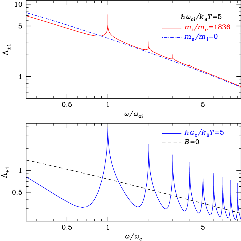
Fig. 4: Electron (lower panel) and proton (upper panel) cyclotron harmonics of the Coulomb logarithm for free-free absorption at $\hbar\omega_{\mathrm{c}}=5k_{\mathrm{B}}T$ and $\hbar\omega_{\mathrm{ci}}=5k_{\mathrm{B}}T$, respectively, for the photon polarization across the magnetic field. Solid lines show the result of the accurate calculation of $\Lambda_{1}(\omega)=\Lambda_{-1}(\omega)$ in the Born approximation, and dot-dashed line in the upper panel shows the infinite-proton-mass approximation (in the lower panel it effectively coincides with the accurate result). For comparison, the dashed line in the lower panel shows the nonmagnetic Coulomb logarithm.

5.3 Atoms

As first noticed in [270], atoms with bound states should be much more abundant at $\gamma\gg 1$ than at $\gamma\lesssim 1$ in a neutron-star atmosphere at the same temperature. This difference is caused by the magnetically-induced increase of binding energies and decrease of sizes of atoms in so-called tightly-bound states, which are characterized by electron-charge concentration at short distances to the nucleus. Therefore it is important to take account of the bound states and bound-bound transitions in a strong magnetic field even for light-element atmospheres, which would be almost fully ionized in the nonmagnetic case.

Pioneering works by Loudon, Hasegawa and Howard [271, 272] were at the origin of numerous studies of atoms in strong magnetic fields. In most of these studies the authors used the model of an atom with an infinitely heavy (fixed in space) nucleus. Their results are summarized in a number of reviews (e.g., [273, 274]). The model of an infinitely massive nucleus is too crude to describe the atoms in the strongly magnetized neutron-star atmospheres, but it is a convenient first approximation. Therefore, in this section we keep to this model, and postpone going beyond its frames to § 5.6.

According to the Thomas-Fermi model, a typical size of an atom with a large nuclear charge $Z_{\mathrm{n}}\gg 1$ is proportional to $\gamma^{-2/5}$ in the interval $Z_{\mathrm{n}}^{4/3}\ll\gamma\ll Z_{\mathrm{n}}^{3}$ [275]. At $\gamma\gtrsim Z_{\mathrm{n}}^{3}$, the usual Thomas-Fermi model becomes inapplicable for an atom [276]. In particular, it cannot describe the difference of the transverse and longitudinal atomic sizes, which becomes huge in such strong fields. In this field range, however, a good starting approximation is provided by so called adiabatic approximation, which presents each electron orbital as a product of a Landau function [256], describing free electron motion in the plane transverse to the field, and a function describing a one-dimensional motion of the electron along magnetic field lines in the field of an effective potential, similar to the Coulomb potential truncated at zero [277]. At $\gamma\gg Z_{\mathrm{n}}^{3}$, all electron shells of the atom are strongly compressed in the directions transverse to the field. In the ground state, atomic sizes along and transverse to $\bm{B}$, respectively, can be estimated as [278]

$$l_{\perp}\approx\sqrt{2Z_{\mathrm{n}}-1}\,a_{\mathrm{m}},\quad l_{\|}\approx\frac{Z_{\mathrm{n}}^{-1}a_{\mathrm{B}}}{\ln[\sqrt{\gamma}/(Z_{\mathrm{n}}\sqrt{2Z_{\mathrm{n}}-1})]}.$$ (48)

In this case, the binding energy $E^{(0)}$ of the ground state increases with increasing $\bm{B}$ approximately as $(\ln\gamma)^{2}$. Here and hereafter, the superscript (0) indicates the approximation of a nonmoving nucleus. At $Z_{\mathrm{n}}\gg 1$ and $\gamma/Z_{\mathrm{n}}^{3}\to\infty$, the asymptotic estimate reads $E^{(0)}\sim-Z_{\mathrm{n}}\hbar^{2}/(m_{\mathrm{e}}l_{\|}^{2})$ [278]. However, this asymptote is never reached in practice (see § 5.5).

Particularly many works were devoted to the simplest atom in magnetic field, the H atom. Since the electron resides on the ground Landau level $N=0$ in the hydrogen atom at $B>10^{9}$ G, its spin being directed opposite to the field, a bound state is determined by quantum numbers $s$ and $\nu$, where $s=0,1,2,\ldots$ corresponds to the electron orbital-momentum projection on the magnetic-field direction, $-\hbar s$, and $\nu=0,1,2,\ldots$ in the adiabatic approximation is equal to the number of wave-function nodes along this direction. The tightly-bound atomic states are characterized by the value $\nu=0$, while all non-zero values of $\nu$ correspond to loosely-bound states.

Calculations of the hydrogen-atom properties beyond the adiabatic approximation were performed by various methods (variational, discrete-mesh, etc.). At $\gamma\gg 1$, the most natural method of calculations is the expansion of the wave function over the Landau orbitals, which constitute a complete orthogonal functional basis in the plane perpendicular to the magnetic field [279]. Such calculations were done in [279, 280, 281] for the bound states and in [282] also for the continuum states, which allowed one to obtain the oscillator strengths as well as photoionization cross-sections. Examples of such cross-sections are presented in Fig. 5 for the hydrogen atom at rest in strong magnetic fields with account of the finite proton mass. The broad peaks correspond to transitions to excited Landau levels $N>0$, while the narrow peaks and dips near corresponding partial thresholds with $\hbar\omega\approx N\hbar\omega_{\mathrm{c}}$ are due to resonances related to autoionization of metastable states [282].

Fig. 5: Logarithm of photoionization cross-section, normalized to the Thomson cross section (31), $\log(\sigma/\sigma_{\mathrm{T}})$, as function of photon energy $\hbar\omega$ for the ground state of the hydrogen atom at rest in magnetic field $B=10^{11}$ G. The curves labelled by “+”, “$-$”, and “$\|$” display the cross sections for circular and longitudinal polarizations $\alpha=+1$, $-1$, and 0, respectively, and the curve labelled “$\perp$” is for radiation polarized perpendicular to $\bm{B}$. The wave vector $\bm{k}$ is directed along $\bm{B}$ for $\alpha\pm 1$ and perpendicular to $\bm{B}$ for the other two cases. (Fig. 4 from [282], reproduced with the permission of ©ESO.)

Analytical expressions for atomic characteristics are best suited for astrophysical modeling. However, the asymptotic estimates at $\gamma\gg 1$ do not provide the desirable accuracy. For example, the binding energy of the ground-state hydrogen atom at rest, $E^{(0)}_{s\nu}$ at $s=\nu=0$, when calculated in frames of the nonrelativistic quantum mechanics, goes to $(\ln\gamma)^{2}$ Ry in the limit $\gamma\to\infty$ [271, 277], but this estimate is in error by a factor over 2 at any $B$ values that are encountered in the neutron stars. With account of two further terms of the asymptotic expansion [272] $E^{(0)}_{00}\sim\ln^{2}(\tilde{\gamma}/\ln^{2}\tilde{\gamma})$ Ry, where $\tilde{\gamma}\approx 0.28\gamma$. But even this estimate differs from accurate results by 40 – 80 % at $B\sim 10^{12}$ – $10^{14}$ G. A possible way of solution to this problem consists in constructing analytical approximations to the results of numerical calculations. In [283] we gave accurate fitting formulae for many bound states of the hydrogen atom at $B\lesssim 10^{14}$ G. The energy levels in the infinite-mass approximation have been recently revisited by Popov and Karnakov [284], who obtained analytical expressions, applicable at $B\gtrsim 10^{11}$ G. Here we will give another approximation for the tightly-bound levels, valid at any $B$. Temporarily ignoring corrections for vacuum polarization (§ 5.5) and finite nuclear mass (§ 5.6), we present the binding energy as

$$\frac{E_{s,0}^{(0)}}{\mbox{Ry}}=\frac{(1+s)^{-2}+(1+s)\,x/a_{1}+a_{3}x^{3}+a_{4}x^{4}+a_{6}x^{6}}{1+a_{2}x^{2}+a_{5}x^{3}+a_{6}x^{4}},$$ (49)

where $x=\ln(1+a_{1}\gamma)$. Here, $a_{i}$ are numerical parameters, which we approximate as functions of $s$:

$$a_{1} = {(0.862+2.5\,s^{2})}/{(1+0.018\,s^{3})}\,,$$

$$a_{2} = 0.275+0.1763\,\delta_{s,0}+s^{2.5}/6\,,$$

$$a_{3} = 0.2775+0.0202\,s^{2.5},\qquad$$

$$a_{4} = {0.3157}/{(1+2s)^{2}}-0.26\,\delta_{s,0},$$

$$a_{5} = 0.0431,$$

$$a_{6} = {2.075\times 10^{-3}}/{(1+7s^{2})^{0.1}}+1.062\times 10^{-4}\,s^{2.5}\,.$$

Approximation (49) accurately reproduces the Zeeman shift of the lowest sublevel of each multiplet in the weak-field limit and the correct asymptote in the strong-field limit. Its inexactness is confined within 3% for $s<30$ at $\gamma>1$ and for $s<5$ at any $\gamma$, and within 0.3% for $s=0$ at any $\gamma$.

Binding energies of the loosely-bound states ($\nu\geqslant 1$) can be evaluated at $\gamma\gtrsim 1$ as

$$E_{s,\nu}^{(0)}=\frac{\mbox{1~{}Ry}}{(n+\delta)^{2}},$$ (50)

where

$$n=\frac{\nu+1}{2},\quad\delta\approx\frac{1+s/2}{1+2\sqrt{\gamma}+0.077\gamma}\quad\mbox{for odd $\nu$;}$$

$$n=\frac{\nu}{2},\quad\delta\approx\frac{1+s/8}{0.6+1.28\ln(1+0.7\gamma^{1/3})}\quad\mbox{for even $\nu$.}$$

At $\gamma\to\infty$, energies (50) tend to those of a field-free H atom ($n^{-2}$ Ry), therefore the loosely-bound states are often called “hydrogenlike” (this picture is broken by vacuum polarization, § 5.5).

In the approximation of an infinite nuclear mass, the energy of any one-electron ion is related to the hydrogen atom energy as $E(Z_{\mathrm{n}},B)=Z_{\mathrm{n}}^{2}\,E(1,B/Z_{\mathrm{n}}^{2})$ [285]. Thus one sees, in particular, that the adiabatic approximation for the single-electron ions is applicable at $\gamma\gg Z_{\mathrm{n}}^{2}$, which is a weaker condition than for many-electron atoms. Analogous similarity relations exist also for the cross sections of radiative transitions [286]. However, they are violated if one takes motion across the magnetic field into account. Even for an atom at rest, the account of the finite nuclear mass can be important at $s\neq 0$. These effects will be considered in § 5.6.

Binding energies and oscillator strengths of many-electron atoms were successfully calculated with the use of different methods: variational (e.g., [287] and references therein), density-functional [288, 289, 290], Monte Carlo [291, 292], and the Hartree-Fock method [293, 294]. In the simplest version of the Hartree-Fock method [274, 295, 296], the wave-function basis is constructed from the one-electron wave functions in the adiabatic approximation. This method is reliable for calculations of the energies, oscillator strengths, and photoionization cross sections of the helium atom [297]. But for many-electron atoms the condition of applicability of the adiabatic approximation $\gamma\gg Z_{\mathrm{n}}^{3}$ is too restrictive. It is overcome in the mesh Hartree-Fock method, where each one-electron orbital is numerically determined as a function of the longitudinal ($z$) and radial coordinates on a two-dimensional mesh [298] (see also [299], and references therein), and in the “twice self-consistent” method [300], where a transverse part of each orbital is presented as a linear superposition of the Landau functions with numerically optimized coefficients. These works gave a number of important results but were not realized in astrophysical applications. In practice, the optimal method for modeling neutron-star atmospheres containing atoms and ions of elements with $2<Z_{\mathrm{n}}\lesssim 10$ proves to be the method by Mori and Hailey [301], where corrections to the adiabatic Hartree approximation are treated by perturbation. The latter method can provide an acceptable accuracy at moderate computational expenses.

5.4 Molecules and molecular ions

Molecular properties in strong magnetic fields have been studied during almost 40 years, but remain insufficiently known. Known the best are the properties of diatomic molecules oriented along the field, especially the H₂ molecule (see [302], and references therein). Lai [303] obtained approximate expressions for its binding energy at $\gamma\gtrsim 10^{3}$, which grows approximately at the same rate $\propto(\ln\gamma)^{2}$ as the atomic binding energy. In such strong fields, the ground state of this molecule is the state where the spins of both electrons are opposite to the magnetic field and the molecular axis is parallel to it, unlike the weak fields where the ground state is ${}^{1}\Sigma_{g}$. In moderate fields, the behavior of the molecular terms is quite nontrivial. If the molecular axis is parallel to $\bm{B}$, then the states ${}^{1}\Sigma_{g}$ and ${}^{3}\Pi_{u}$ are metastable at $0.18<\gamma<12.3$, and decay into the channel ${}^{3}\Sigma_{u}$ [304]. It turns out, however, that the molecular orientation along $\bm{B}$ is not optimal in such fields: for example, at $\gamma=1$ the triplet state of the molecule oriented perpendicular to the field has the lowest energy, and at $\gamma=10$ the ground state is inclined at 37^∘ to $\bm{B}$ [305].

The ion H₂⁺ is well studied, including its arbitrary orientations in a magnetic field (e.g., [306], and references therein). An analysis by Khersonskii [307] shows that the abundance of H₂⁺ is very small in neutron-star atmospheres, therefore the these ions are unlikely to affect the observed spectra.

Strong magnetic fields stabilize the molecule He₂ and its ions He₂⁺, He₂²⁺, and He₂³⁺, which do not exist in the absence of the field. Mori and Heyl [308] have performed the most complete study of their binding energies in neutron-star atmospheres. The ions HeH⁺⁺, H₃⁺⁺, and other exotic molecular ions, which become stable in the strong magnetic fields, were also considered (see [309, 310], and references therein). Having evaluated the ionization equilibrium by the Khersonskii’s method [307], one can easily see that the abundance of such ions is extremely small at the densities, temperatures, and magnetic fields characteristic of the neutron stars. Therefore, such ions do not affect the thermal spectrum.

There are rather few results on molecules composed of atoms heavier than He. Let us note the paper [311], where the authors applied the density-functional method to calculations of binding energies of various molecules from H_n to Fe_n with $n$ from 1 through 8 at $B$ from $10^{12}$ G to $2\times 10^{15}$ G. The earlier studies of heavy molecules in strong magnetic fields are discussed in the review by Lai [303]. All these studies assumed the model of infinitely massive atomic nuclei.

5.5 Relativistic effects

One can encounter the statement that the use of the nonrelativistic quantum mechanics for calculation of atomic and molecular structure is justified only at $B<B_{\mathrm{QED}}$. However, a treatment of the hydrogen atom in strong magnetic fields based on the Dirac equation [312, 313, 314] has not revealed any significant differences from the solution to the same problem based on the Schrödinger equation. The reasons for that are clear. One can always expand a wave function over a complete basis of two-dimensional functions, such as the set of the Landau functions for all electrons. The Landau functions have the same form in the relativistic and nonrelativistic theories [256]. Coefficients of such expansion are functions of $z$ corresponding to the electron motion along $\bm{B}$. This motion is nonrelativistic for the bound electrons, because the maximal binding energy is much smaller than the electron rest energy $m_{\mathrm{e}}c^{2}=511$ keV. Therefore, a system of equations for the functions of $z$ in question can be solved in the nonrelativistic approximation, which thus provides the accurate wave function.

Nevertheless, there is a specific relativistic effect, which is non-negligible in superstrong fields. As noted by Heisenberg and Euler [315], the virtual electron-positron pairs that appear in an electromagnetic field according to the Dirac theory, modify the Maxwell equations. This effect is called vacuum polarization. To date it has not been observed, but it was studied in many theoretical works, reviewed in detail by Schubert [316]. A strong electromagnetic field creates a nonzero space charge by acting on the virtual pairs. Such charge, in particular, screens the Coulomb interaction between an electron and an atomic nucleus at distances comparable to the Compton wavelength $\lambda_{\mathrm{C}}=2\pi\hbar/(m_{\mathrm{e}}c)=2\pi\alpha_{\mathrm{f}}a_{\mathrm{B}}$. Shabad and Usov [317, 318] noted that this screening affects the even atomic levels in superstrong magnetic fields, which squeeze the atom so that its size becomes comparable to $\lambda_{\mathrm{C}}$. As a result, instead of the unlimited growth of the binding energies of the tightly-bound states that is predicted by the nonrelativistic theory for unlimited increase of $B$, these energies ultimately level off. For the same reason, the double degeneracy of the loosely-bound states that follows from Eq. (50) at $\gamma\to\infty$, does not realize.

Machet and Vysotsky [319] have thoroughly studied this effect, confirmed the qualitative conclusions of Shabad and Usov, and obtained more accurate quantitative estimates. In particular, according to their results (see also [284]), the effect of the vacuum polarization on the electron binding energies in a nonmoving Coulomb potential can be simulated by replacing the parameter $\gamma$ to $\gamma^{\ast}=\gamma/[1+\alpha_{\mathrm{f}}^{3}\gamma/(3\pi)]$. As a result, the binding energy of the hydrogen atom cannot exceed 1.71 keV at any $B$.

5.6 The effects of finite nuclear mass

An overwhelming majority of studies of atoms in strong magnetic fields assumed the nuclei to be infinitely massive (fixed in space). For magnetic neutron-star atmospheres, this approximation is very serious and often an undesirable simplification.

Let us start with an atom with a nonmoving center of mass. The nucleus of a finite mass, as any charged particle, undergoes circular oscillations in the plane perpendicular to $\bm{B}$. In the atom, these oscillations cannot be separated from the electron oscillations, therefore the longitudinal projections of the orbital moments of the electrons and the nucleus are not conserved separately. Only their difference is conserved. Different atomic quantum numbers correspond to different oscillation energies of the atomic nucleus, multiple of its cyclotron energy. As a result, the energy of every level gets an addition, which is non-negligible if the parameter $\gamma$ is not small compared to the nucleus-to-electron mass ratio. For the hydrogen atom and hydrogenlike ions, $\hbar s$ in Eq. (49) now corresponds to the difference of longitudinal projections of orbital moments of the atomic nucleus and the electron, and the sum $N+s$ plays role of a nuclear Landau number, $N$ being the electron Landau number. For the bound states in strong magnetic fields, $N=0$, therefore the nuclear oscillatory addition to the energy equals $s\hbar\omega_{\mathrm{ci}}$. Thus the binding energy of a hydrogen atom at rest is

$$E_{s\nu}=E_{s\nu}^{(0)}(\gamma^{\ast})-\hbar\omega_{\mathrm{ci}}s,$$ (51)

where $\gamma^{\ast}=\gamma/(1+4.123\times 10^{-8}\,\gamma)$ according to § 5.5. It follows that the number of $s$ values is limited for the bound states. In particular, one can easily check using Eqs. (49) and (51) that all bound states have zero moment-to-field projection ($s=0$) at $B>6\times 10^{13}$ G.

The account of the finite nuclear mass is more complicated for multielectron atoms. Al-Hujaj and Schmelcher [320] have shown that the contribution of the nuclear motion to the binding energy of a non-moving atom equals $\hbar\omega_{\mathrm{ci}}S(1+\delta(\gamma))$, where ($-S$) is the total magnetic quantum number and $|\delta(\gamma)|\ll 1$.

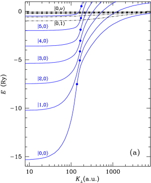
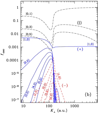
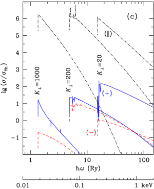
Fig. 6: (a) energies, (b) oscillator strengths, and (c) photoionization cross-sections for a hydrogen atom moving in magnetic field $B=2.35\times 10^{12}$ G. Energies of states $|s,0\rangle$ (solid curves) and $|0,\nu\rangle$ (dot-dashed curves) are shown as functions of the transverse pseudomomentum $K_{\perp}$ (in atomic units). The heavy dots on the solid curves are the inflection points at $K_{\perp}=K_{\mathrm{c}}$. The $K_{\perp}$-dependence of oscillator strengths (b) is shown for transitions from the ground state to the states $|s,0\rangle$ under influence of radiation with polarization $\alpha=+1$ (solid curves) and $\alpha=-1$ (dashed curves), and also for transitions into states $|0,\nu\rangle$ for $\alpha=0$ (dot-dashed curves). Cross sections of photoionization (c) under the influence of radiation with $\alpha=+1$ (solid curves), $\alpha=-1$ (dashed curves), and $\alpha=0$ (dot-dashed curves) are shown for the ground state as functions of the photon energy in Ry (the upper x-scale) and keV (the lower x-scale) at $K_{\perp}=20$ a.u. (the right curve), $K_{\perp}=200$ a.u. (the middle curve), and $K_{\perp}=1000$ a.u. (the left curve of every type).

The astrophysical simulations require an account of finite temperatures, hence thermal motion of particles. The theory of motion of a system of point charges in a constant magnetic field is reviewed in [321, 322]. The canonical momentum $\bm{P}$ is not conserved in this motion, but a pseudomomentum $\bm{K}=\bm{P}+(1/2c)\,\bm{B}\times\sum_{i}q_{i}\bm{r_{i}}$ is conserved. The pseudomomentum of a single charged particle has a one-to-one correspondence to the position of the guiding center in the $(xy)$ plane, perpendicular to the magnetic field, while a pseudomomentum of an atom or ion equals the sum of pseudomomenta of its constituent particles. If the system is electrically neutral as a whole, then all the components of $\bm{K}$ are good quantum numbers. For a charged system (an ion), $K^{2}$ is a good quantum number, while $K_{x}$ and $K_{y}$ do not commute. The specific effects related to collective motion of a system of charged particles are especially important in a neutron-star atmosphere at $\gamma\gg 1$. In particular, so called decentered states may become populated, where an electron is localized mostly in a “magnetic well” aside from the Coulomb center.

For a hydrogen atom, $\bm{K}=\bm{P}+({e}/{2c})\,\bm{B}\times\bm{R},$ where the vector $\bm{R}$ connects the electron to the proton. The studies of this particular case were initiated in the pioneering works [323, 324, 325]. Numerical calculations of the energy spectrum of the hydrogen atom with account of the effects of motion across a strong magnetic field were performed in [326, 327]. Probabilities of various radiative transitions were studied in a series of papers ended with [258].

Figure 6 shows the energies, oscillator strengths, and photoionization cross-sections of a hydrogen atom moving in a magnetic field with $\gamma=1000$. The negative energies in Fig. 6a correspond to bound states. The reference point is taken to be the sum of the zero-point oscillation energies of free electron and proton, $(\hbar\omega_{\mathrm{c}}+\hbar\omega_{\mathrm{ci}})/2$. At small transverse pseudomomenta $K_{\perp}$, the energies of low levels in Fig. 6a exceed the binding energy of the field-free hydrogen atom (1 Ry) by an order of magnitude. However, the total energy increases with increasing $K_{\perp}$, and it can become positive for the states with $s\neq 0$ due to the term $\hbar\omega_{\mathrm{ci}}s$ in Eq. (51). Such states are metastable. In essence, they are continuum resonances. Note that the transverse atomic velocity equals $\partial E/\partial\bm{K}$, therefore it is maximal at the inflection points ($K_{\perp}=K_{\mathrm{c}}$) on the curves in Fig. 6a and decreases with further increase of $K_{\perp}$ [327], while the average electron-proton distance continues to increase. The atom goes into the decentered state, where the electron and proton are localized near their guiding centers, separated by distance $r_{*}=(a_{\mathrm{B}}^{2}/\hbar)K_{\perp}/\gamma$.

The dependences of the binding energies on $K_{\perp}$ are approximately described at $K_{\perp}\ll K_{\mathrm{c}}$ and $K_{\perp}\gg K_{\mathrm{c}}$, respectively, by expressions

$$E_{s\nu}^{(<)} \!\!= \!\!E_{s\nu}^{(0)}-K_{\perp}^{2}/(2m_{\mathrm{eff}})-\hbar\omega_{\mathrm{ci}}s,$$ (52)

$$E_{s\nu}^{(>)} \!\!\!\!\!= \!\!\!\!\!\frac{\mbox{2\,Ry}}{\sqrt{\hat{r}_{*}^{2\phantom{/}}+(2\nu+1)\,\hat{r}_{*}^{3/2}+\ldots}}-\hbar\omega_{\mathrm{ci}}s\,,$$ (53)

where $\hat{r}_{*}\equiv r_{*}/a_{\mathrm{B}}$ and $m_{\mathrm{eff}}$ is an effective “transverse mass.” The latter is expressed through the values of $E_{s\nu}^{(0)}$ for the given and neighboring levels by the perturbation theory [328, 329]. However, for excited states even a small inaccuracy in $E_{s\nu}^{(0)}$ may lead to a fatal error in $m_{\mathrm{eff}}$. Therefore in practice it is more convenient to use the approximation $m_{\mathrm{eff}}\approx m_{\mathrm{a}}\,[1+(\gamma/\gamma_{s\nu})^{p_{s\nu}}]$, where $\gamma_{s\nu}$ and $p_{s\nu}$ are dimensionless parameters, and $m_{\mathrm{a}}$ is the true mass of the atom. For the tightly bound levels, $\gamma_{s0}\approx 6\times 10^{3}/(1+2s)^{2}$ and $p_{s\nu}\approx 0.9$. At $B\lesssim 10^{13}$ G we can approximately describe the energies of the states with $\nu=0$ at arbitrary $K_{\perp}$, if we replace the ellipsis under the square root in Eq. (53) by the expression $\hat{r}_{*}/(5+3s)+\big{(}\mbox{2~{}Ry}/E_{s\nu}^{(0)}\big{)}^{2}$, and replace the inflection point $K_{\mathrm{c}}$ by intersection of $E_{s\nu}^{(<)}(K_{\perp})$ with $E_{s\nu}^{(>)}(K_{\perp})$. At stronger fields or for $\nu\neq 0$, the transition between the centered and decentered states smears, and one has to resort to more complex fitting formulae [283].

Figure 6b shows oscillator strengths for the main dipole-allowed transitions from the ground state to excited discrete levels as functions of $K_{\perp}$. Since the atomic wave-functions are symmetric with respect to the $z$-inversion for the states with even $\nu$, and antisymmetric for odd $\nu$, only the transitions that change the parity of $\nu$ are allowed for the polarization along the field ($\alpha=0$), and only those preserving the parity for the orthogonal polarizations ($\alpha=\pm 1$). For the atom at rest, in the dipole approximation, due to the conservation of the $z$-projection of the total angular momentum of the system, absorption of a photon with polarization $\alpha=0,\pm 1$ results in the change of $s$ by $\alpha$. This selection rule for a non-moving atom manifests itself in vanishing oscillator strengths at $K_{\perp}\to 0$ for $s\neq\alpha$. In an appropriate coordinate system [324, 327], the symmetry is restored at $K_{\perp}\to\infty$, therefore the transition with $s=\alpha$ is the only one that survives also in the limit of large pseudomomenta. But in the intermediate region of $K_{\perp}$, where the transverse atomic velocity is not small, the cylindrical symmetry is broken, so that transitions to other levels are allowed. Thus the corresponding oscillator strengths in Fig. 6b have maxima at $K_{\perp}\approx K_{\mathrm{c}}$. Analytical approximations for these oscillator strengths are given in [283].

Figure 6c shows photoionization cross-sections for hydrogen in the ground state as functions of photon energy at three values of $K_{\perp}$. The leftward shift of the ionization threshold with increasing $K_{\perp}$ corresponds to the decrease of the binding energy that is shown in Fig. 6a, while the peaks and dips on the curves are caused by resonances at transitions to metastable states $|s,\nu;K\rangle$ with positive energies (see [258], for a detailed discussion).

Quantum-mechanical calculations of the characteristics of the He⁺ ion that moves in a strong magnetic field are performed in [330, 331]. The basic difference from the case of a neutral atom is that the the ion motion is restricted by the field in the transverse plane, therefore the values of $K^{2}$ are quantized [321, 322]. Clearly, the similarity relations for the ions with nonmoving nuclei (§ 5.3) do not hold anymore.

Currently there is no detailed calculation of binding energies, oscillator strengths, and photoionization cross-sections for atoms and ions other than H and He⁺, arbitrarily moving in a strong magnetic field. For such species one usually neglects the decentered states and uses a perturbation theory with respect to $K_{\perp}$ [328, 329]. Such approach was realized, e.g., in [301, 297]. It can be sufficient for simulations of relatively cool atmospheres of moderately magnetized neutron stars. Detailed conditions of applicability of the perturbation theory [328, 329] require calculations, but a rough order-of-magnitude estimate can be obtained by requiring that the mean Lorentz force acting on a bound electron because of the atomic thermal motion should be small compared to the Coulomb forces. As a result, for an atom with mass $m_{\mathrm{a}}=Am_{\mathrm{u}}$ we get the condition $k_{\mathrm{B}}T/E_{\mathrm{b}}\ll m_{\mathrm{a}}/(\gamma m_{\mathrm{e}})\approx 4A/B_{12}$, where $E_{\mathrm{b}}$ is the atomic ionization energy. If $B\lesssim 10^{13}$ G and $T\lesssim 10^{6}$ K, it is well satisfied for low-lying levels of carbon and heavier atoms.

5.7 Equation of state

Theoretical description of thermodynamics of partially ionized plasmas can be based on either “physical” of “chemical” models (see, e.g., a discussion and references in [332, 333]). In the chemical model of plasmas, bound states (atoms, molecules, ions) are treated as separate members of the thermodynamic ensemble, while in the physical model the only members of the ensemble are atomic nuclei and electrons. Each of the models can be thermodynamically self-consistent, but the physical model is more relevant from the microscopic point of view, because it does not require a distinction of electrons bound to a given nucleus. Such a distinction becomes very ambiguous at high densities, where several nuclei can attract the same electron with comparable forces. On the other hand, calculations in frames of the physical model are technically more complicated. As a rule, they are based on a diagram expansion, which requires an increase of the number of terms with the density increase. For this reason, even the most advanced equation of state for nonmagnetic photospheres that is based on the physical model [334] still restricts to the domain $\rho\lesssim 10\,T_{6}^{3}$ g cm^-3.

Studies of magnetic neutron-star photospheres, as a rule, are based on the chemical plasma model. In this case, the ionization equilibrium is evaluated by minimizing the Helmholtz free energy $F$ given by

$$F=F_{\mathrm{id}}^{(e)}+F_{\mathrm{id}}^{\mathrm{(i)}}+F_{\mathrm{int}}+F_{\mathrm{ex}},$$ (54)

where $F_{\mathrm{id}}^{(e)}$ and $F_{\mathrm{id}}^{(i)}$ describe the ideal electron and ion gases, $F_{\mathrm{int}}$ includes internal degrees of freedom for bound states, and $F_{\mathrm{ex}}$ is a nonideal component. All thermodynamic functions that are required for modeling a photosphere with a given chemical composition are expressed through derivatives of $F$ over $\rho$ and $T$ [335].

According to the Bohr-van Leeuwen theorem, magnetic field does not affect thermodynamics of classical charged particles. The situation differs in the quantum mechanics. The importance of the quantum effects depends on the parameters $\zeta_{\mathrm{e}}$ (40) and $\zeta_{\mathrm{i}}$ (41).

We use the equality [335] $F_{\mathrm{id}}^{(e)}/V=\mu_{\mathrm{e}}n_{\mathrm{e}}-P_{\mathrm{id}}^{(e)}$ where $V$ is the volume of the system, and $\mu_{\mathrm{e}}$, $n_{\mathrm{e}}$, and $P_{\mathrm{id}}^{\mathrm{(e)}}$ are, respectively, the chemical potential, number density, and pressure in the ideal electron gas model. The equation of state is determined by a relation between these quantities, which can be found from relations (e.g., [1, 90])

$$\Bigg{\{}\begin{array}[]{l}n_{\mathrm{e}}\\ P_{\mathrm{id}}^{(e)}\end{array}\Bigg{\}}=\sum_{N,\sigma}\frac{(1+2bN)^{1/4}}{\pi^{3/2}a_{\mathrm{m}}^{2}\lambda_{\mathrm{e}}}\Bigg{\{}\begin{array}[]{l}{\partial I_{1/2}(\chi_{N},\tau_{N})}/{\partial\chi_{N}}\\ k_{\mathrm{B}}T\,I_{1/2}^{\phantom{I}}(\chi_{N},\tau_{N})\end{array}\Bigg{\}},$$ (55)

where $\lambda_{\mathrm{e}}=[{2\pi\hbar^{2}}/({m_{\mathrm{e}}k_{\mathrm{B}}T})]^{1/2}$ is the thermal de Broglie wavelength, $\tau_{N}=k_{\mathrm{B}}T/(m_{\mathrm{e}}c^{2}\sqrt{1+2bN})$, $\chi_{N}=\mu_{\mathrm{e}}/(k_{\mathrm{B}}T)+\tau_{0}^{-1}-\tau_{N}^{-1}$,

$$I_{1/2}(\chi_{N},\tau_{N})\equiv\int_{0}^{\infty}\frac{\sqrt{x\,(1+\tau_{N}x/2)}}{\exp(x-\chi_{N})+1}\,{\mathrm{d}}x$$ (56)

is the Fermi-Dirac integral, and the summation is done over all $N$ and all values of spin projections on the magnetic field, $\hbar\sigma/2$, so that $\sigma=\pm 1$ for positive $N$ and $\sigma=-1$ at $N=0$.

In a strongly quantizing magnetic field, it is sufficient to retain only the term with $N=0$ in the sums (55). In this case, the electron Fermi momentum equals $p_{\mathrm{F}}=2\pi^{2}a_{\mathrm{m}}^{2}\hbar n_{\mathrm{e}}$. Therefore, with increasing $n_{\mathrm{e}}$ at a fixed $B$, the degenerate electrons begin to fill the first Landau level when $n_{\mathrm{e}}$ reaches $n_{B}=(\pi^{2}\sqrt{2}\,a_{\mathrm{m}}^{3})^{-1}$. This value just corresponds to the density $\rho_{B}$ in Eq. (39). The ratio of the Fermi momentum $p_{\mathrm{F}}$ in the strongly quantizing field to its nonmagnetic value $\hbar(3\pi^{2}n_{\mathrm{e}})^{1/3}$ equals $[{4\rho^{2}}/{(3\rho_{B}^{2})}]^{1/3}$. Therefore, the Fermi energy at a given density $\rho<\sqrt{3/4}\,\rho_{B}$ becomes smaller with increasing $B$, that is, a strongly quantizing magnetic field relieves the electron-gas degeneracy. For this reason, strongly magnetized neutron-star photospheres remain mostly nondegenerate, as it were in the absence of the field, despite their densities are orders of magnitude higher than the nonmagnetic photosphere densities.

The free energy of nondegenerate nonrelativistic ions is given by

$$\frac{F_{\mathrm{id}}^{\mathrm{(i)}}}{N_{\mathrm{i}}k_{\mathrm{B}}T} = \ln\left(2\pi\frac{n_{\mathrm{i}}\lambda_{\mathrm{i}}a_{\mathrm{m}}^{2}}{Z}\right)+\ln\left(1-\mathrm{e}^{-\zeta_{\mathrm{i}}}\right)-1$$ (57)

$$+\frac{\zeta_{\mathrm{i}}}{2}+\ln\Bigg{(}\frac{\sinh[g_{\mathrm{i}}\,\zeta_{\mathrm{i}}(2s_{\mathrm{i}}+1)/4]}{\sinh(g_{\mathrm{i}}\,\zeta_{\mathrm{i}}/4)}\Bigg{)},$$

where $\lambda_{\mathrm{i}}=[2\pi\hbar^{2}/(m_{\mathrm{i}}k_{\mathrm{B}}T)]^{1/2}$ is the thermal de Broglie wavelength for the ions, $s_{\mathrm{i}}$ is the spin number, and $g_{\mathrm{i}}$ is the spin-related g-factor (for instance, $s_{\mathrm{i}}=1/2$ and $g_{\mathrm{i}}=5.5857$ for the proton). All the terms in (57) have clear physical meanings. At $\zeta_{\mathrm{i}}\to 0$, the first and second terms give together $\ln(n_{\mathrm{i}}\lambda_{\mathrm{i}}^{3})$, which corresponds to the three-dimensional Boltzmann gas. The first term corresponds to the one-dimensional Boltzmann gas model at $\zeta_{\mathrm{i}}\gg 1$. The second-last term in (57) gives the total energy $N_{\mathrm{i}}\hbar\omega_{\mathrm{ci}}/2$ of zero-point oscillations transverse to the magnetic field. Finally, the last term represents the energy of magnetic moments in a magnetic field.

The nonideal free-energy part $F_{\mathrm{ex}}$ contains the Coulomb and exchange contributions of the electrons and the ions, and the electron-ion polarization energy. In the case of incomplete ionization $F_{\mathrm{ex}}$ includes also interactions of ions and electrons with atoms and molecules. In turn, the interaction between the ions is described differently depending on the phase state of matter. The terms that constitute $F_{\mathrm{ex}}$ depend on magnetic field only if it quantizes the motion of these interacting particles. Here we will not discuss these terms but address an interested reader to the paper [90] and references therein. This nonideality is negligible in the neutron-star atmospheres, but it determines the formation of a condensed surface, which will be considered in § 5.10.

5.8 Ionization equilibrium

For photosphere simulations, it is necessary to determine the fractions of different bound states, because they affect the spectral features that are caused by bound-bound and bound-free transitions. Solution to this problem is laborious and ambiguous. The principal difficulty in the chemical plasma model, namely the necessity to distinguish the bound and free electrons and “attribute” the bound electrons to certain nuclei, becomes especially acute at high densities, where the atomic sizes cannot be anymore neglected with respect to their distances. Current approaches to the solution of this problem are based, as a rule, on the concept of so called occupation probabilities of quantum states. For example, consider electrons in thermodynamic equilibrium with ions of the $Z$th chemical element, and let $j$ be the ionization degree of every ion (i.e., the number of lacking electrons), $\kappa$ is its quantum state, and $E_{j,\kappa}$ and $g_{\kappa}^{(j)}$ are, respectively, its binding energy and statistical weight. An occupation probability $w_{j,\kappa}$ is an additional statistical weight of the given state under the condition of plasma nonideality, that is under interaction of the ion $(Z,j,\kappa)$ with surrounding particles, with respect to its weight without such interactions. As first noted by Fermi [337], occupation probabilities $w_{j,\kappa}$ cannot be arbitrary but should be consistent with $F_{\mathrm{ex}}$. Minimizing $F$ with account of the Landau quantization leads to a system of ionization-equilibrium equations for $n_{j}\equiv\sum_{\kappa}n_{j,\kappa}$ [338, 339]

$$\frac{n_{j}}{n_{j+1}} = n_{\mathrm{e}}\lambda_{\mathrm{e}}^{3}\,\,\frac{\sinh(\zeta_{j}/2)}{\zeta_{j}}\,\frac{\zeta_{j+1}}{\sinh(\zeta_{j+1}/2)}$$ (58)

$$\times\,\frac{\tanh(\zeta_{\mathrm{e}}/2)}{\zeta_{\mathrm{e}}}\,\frac{\mathcal{Z}_{\mathrm{int},j}}{\mathcal{Z}_{\mathrm{int},j+1}}\,\exp\left(\frac{E_{j,\mathrm{ion}}}{k_{\mathrm{B}}T}\right),$$

where $\mathcal{Z}_{\mathrm{int},j}=\sum_{\kappa}g_{\kappa}^{(j)}\,w_{j,\kappa}\,\exp\left[({E_{j,\kappa}-E_{j,\mathrm{gr.st}}})/({{k_{\mathrm{B}}}T})\right]$ is internal partition function for the $j$th ion type, $E_{j,\mathrm{gr.st}}$ is its ground-state binding energy, $E_{j,\mathrm{ion}}=E_{j,\mathrm{gr.st}}-E_{j+1,\mathrm{gr.st}}$ is its ionization energy, and $\zeta_{j}$ is the magnetic quantization parameter (41). Equation (58) differs from the usual Saha equation, first, by the terms with $\zeta_{\mathrm{e}}$ and $\zeta_{j}$, representing partition functions for distributions of free electrons and ions over the Landau levels, and second, by the occupation probabilities $w_{j,\kappa}$ in the expressions for the partition functions $\mathcal{Z}_{\mathrm{int},j}$.

There were many attempts to find such approximation for the occupation probabilities that best reproduced the real plasma EOS. They were discussed, for example, by Hummer and Mihalas [340], who proposed an approximation based on the Inglis-Teller criterion [341] for dissolution of spectral lines because of their smearing due to the Stark shifts in plasma microfields. However, the translation of the spectroscopic criterion to thermodynamics is not well grounded. It is necessary to clearly distinguish between the disappearance of spectral lines of an atom and the complete destruction of this atom with increasing pressure, as was stressed, e.g., in [342, 343, 344]. In order to take this difference into account, in [345] we introduced a concept of optical occupation probabilities $\tilde{w}_{j,\kappa}$, which resemble the Hummer-Mihalas occupation probabilities and should be used for calculation of spectral opacities, but differ from the thermodynamic occupation probabilities $w_{j,\kappa}$ that are used in the EOS calculations.

Equation (58) was applied to modeling partially ionized atmospheres of neutron stars, composed of iron, oxygen, and neon [346, 339, 347, 348]. The effects related to the finite nuclear masses (§ 5.6) were either ignored or treated in the first order of the perturbation theory. Since quantum-mechanical characteristics of an atom in a strong magnetic field depend on the transverse pseudomomentum $K_{\perp}$, the atomic distribution over $K_{\perp}$ cannot be written in a closed form, and only the distribution over longitudinal momenta $K_{z}$ remains Maxwellian. The first complete account of these effects has been taken in [349] for hydrogen photospheres. Let $p_{s\nu}(K_{\perp})\,\mathrm{d}^{2}K_{\perp}$ be the probability of finding a hydrogen atom in the state $|s,\nu\rangle$ in the element $\mathrm{d}^{2}K_{\perp}$ near $\bm{K}_{\perp}$ in the plane of transverse pseudomomenta. Then the number of atoms in the element $\mathrm{d}^{3}K$ of the pseudomomentum space equals

$$\mathrm{d}N(\bm{K})=N_{s\nu}\,\frac{\lambda_{\mathrm{a}}}{2\pi\hbar}\,\exp\left(-\frac{K_{z}^{2}}{2m_{\mathrm{a}}k_{\mathrm{B}}T}\right)\,p_{s\nu}(K_{\perp})\mathrm{d}^{3}K,$$ (59)

where $m_{\mathrm{a}}$ is the mass of the atom, $\lambda_{\mathrm{a}}=[{2\pi\hbar^{2}}/({m_{\mathrm{a}}k_{\mathrm{B}}T})]^{1/2}$ is its thermal wavelength, and $N_{s\nu}=\int\mathrm{d}N_{s\nu}(\bm{K})$ is the total number of atoms with given discrete quantum numbers. The distribution $N_{s\nu}p_{s\nu}(K_{\perp})$ is not known in advance, but should be calculated in a self-consistent way by minimization of the free energy including the nonideal terms. It is convenient to define deviations from the Maxwell distribution with the use of generalized occupation probabilities $w_{s\nu}(K_{\perp})$. Then the atomic contribution $(F_{\mathrm{id}}+F_{\mathrm{int}})$ to the free energy equals [349]

$$k_{\mathrm{B}}T\sum_{s\nu}N_{s\nu}\int\ln\left[n_{s\nu}\lambda_{\mathrm{a}}^{3}\frac{w_{s\nu}(K_{\perp})}{\exp(1)\mathcal{Z}_{s\nu}}\right]p_{s\nu}(K_{\perp})\,\mathrm{d}^{2}K_{\perp},$$ (60)

where

$$\mathcal{Z}_{s\nu}=\frac{\lambda_{\mathrm{a}}^{2}}{(2\pi\hbar^{2})}\int_{0}^{\infty}w_{s\nu}(K_{\perp})\mathrm{e}^{E_{s\nu}(K_{\perp})/k_{\mathrm{B}}T}K_{\perp}\mathrm{d}K_{\perp}.$$ (61)

The nonideal part of the free energy that describes atom-atom and atom-ion interactions and is responsible for the pressure ionization has been calculated in [349] with the use of the hard-sphere model. The plasma model included also hydrogen molecules H₂ and chains H_n, which become stable in the strong magnetic fields. For this purpose, approximate formulae of Lai [303] have been used, which do not take full account of the motion effects, therefore the results of [349] are reliable only when the molecular fraction is small.

This hydrogen-plasma model underlies thermodynamic calculations of hydrogen photospheres of neutron stars with strong [266] and superstrong [350] magnetic fields. Mori and Heyl [308] applied the same approach with slight modifications to strongly magnetized helium plasmas. One of the modifications was the use of the plasma microfield distribution from [226] for calculation of $w(K_{\perp})$. Mori and Heyl considered atomic and molecular helium states of different ionization degrees. Their treated rotovibrational molecular levels by perturbation theory and considered the dependence of binding energies on orientation of the molecular axis relative to $\bm{B}$. The $K_{\perp}$-dependence of the energy, $E(K_{\perp})$, was described by an analytical fit, based on an extrapolation of adiabatic calculations at small $K_{\perp}$. The motion effects of atomic and molecular ions were not considered.

5.9 Applicability of the LTE approximation

The models of EOS and ionization balance usually assume that the LTE conditions are satisfied for the atoms and ions. In particular, the Boltzmann distribution over the Landau levels is assumed. This assumption does not apply for free electrons in the neutron-star atmospheres, if the spontaneous radiative decay rate of excited Landau levels,

$$\Gamma_{\mathrm{r}}=\frac{4}{3}\,\frac{e^{2}\omega_{\mathrm{c}}^{2}}{m_{\mathrm{e}}c^{3}}=3.877\times 10^{15}B_{12}^{2}\mbox{ s}^{-1},$$ (62)

exceeds the rate of their collisional de-excitation.

In a nonquantizing field, the characteristic frequency of electron-ion Coulomb collisions equals (see, e.g., [351])

$$\Gamma_{\mathrm{c}}=\frac{4\sqrt{2\pi}n_{\mathrm{i}}Z^{2}e^{4}\Lambda_{\mathrm{c}}}{3\sqrt{m_{\mathrm{e}}}(k_{\mathrm{B}}T)^{3/2}}=2.2\times 10^{15}\,\frac{Z^{2}}{A}\,\frac{\rho^{\prime}\Lambda_{\mathrm{c}}}{T_{6}^{3/2}}\mbox{ s}^{-1},$$ (63)

where $\rho^{\prime}\equiv\rho/$g cm^-3, and $\Lambda_{\mathrm{c}}$ is a Coulomb logarithm, which weakly depends on $T$ and $\rho$ and usually has an order of magnitude of 1 – 10. In a quantizing field, the electrons are de-excited from the first Landau level by electron-ion Coulomb collisions at the rate

$$\Gamma_{10} \!\!\!\!= \!\!\!\!\frac{4\sqrt{2\pi}\,n_{\mathrm{i}}Z^{2}e^{4}\tilde{\Lambda}_{10}}{\sqrt{m_{\mathrm{e}}}\,\,(\hbar\omega_{\mathrm{c}})^{3/2}}=4.2\times 10^{12}\,\frac{Z^{2}}{A}\,\frac{\rho^{\prime}\tilde{\Lambda}_{10}}{B_{12}^{3/2}}\mbox{~{}s}^{-1}$$ (64)

$$=4.9\times 10^{13}\,\frac{Z^{2}}{A}\frac{\rho^{\prime}\Lambda_{10}}{B_{12}\sqrt{T_{6}}}\mbox{~{}s}^{-1},$$

where $\tilde{\Lambda}_{10}=\sqrt{\zeta_{\mathrm{e}}}\Lambda_{10}$ is a new Coulomb logarithm, which has an order of unity at $\zeta_{\mathrm{e}}\gg 1$, whereas $\Lambda_{10}$ has that order at $\zeta_{\mathrm{e}}\ll 1$ [268]. Note that the rate of the inverse process of collisional excitation equals $\Gamma_{01}=\Gamma_{10}\,\mathrm{e}^{-\zeta_{\mathrm{e}}}$. Comparing (62) and (64), we see that in the weak-field ($B\lesssim 10^{10}$ G) photospheres of isolated neutron stars, at typical $\rho\gtrsim 10^{-3}$ g cm^-3 and $T_{6}\sim 1$, the LTE conditions are fulfilled (it may not be the case in the magnetosphere due to the lower densities). In a strong field ($B\gtrsim 10^{11}$ G), the LTE is violated, and the fraction of electrons on the excited Landau levels is lower than the Boltzmann value $\mathrm{e}^{-\zeta_{\mathrm{e}}}$. However, this does not entail any consequence for the atmosphere models, because in the latter case $\mathrm{e}^{-\zeta_{\mathrm{e}}}$ is vanishingly small.

For the ions, the spontaneous decay rate of the excited Landau levels $\Gamma_{\mathrm{ri}}$ differs from $\Gamma_{\mathrm{r}}$ by a factor of $Z\,(Zm_{\mathrm{e}}/m_{\mathrm{i}})^{3}\sim 10^{-10}$. The statistical distribution of ions over the Landau levels has been studied in [268]. The authors showed that the fraction of the ions on the first excited Landau level is accurately given by

$$\frac{n_{1}}{n_{0}}=\mathrm{e}^{-\zeta_{\mathrm{i}}}\,\frac{1+\epsilon\,(\Gamma_{\mathrm{ri}}/\Gamma_{\mathrm{10,i}})/(1-\mathrm{e}^{-\zeta_{\mathrm{i}}})}{1+\Gamma_{\mathrm{ri}}/\Gamma_{\mathrm{10,i}}+\epsilon\,(\Gamma_{\mathrm{ri}}/\Gamma_{\mathrm{10,i}})/(\mathrm{e}^{\zeta_{\mathrm{i}}}-1)},$$ (65)

where $\epsilon=J_{\omega}/\mathcal{B}_{\omega,T}$ at $\omega=\omega_{\mathrm{ci}}$, and $\Gamma_{\mathrm{10,i}}$ is the collisional frequency of the first level, which differs from Eq. (64) by the factor $\sqrt{m_{\mathrm{i}}/m_{\mathrm{e}}}$ and the value of the Coulomb logarithm. The parameter $\epsilon$ is small in the outer layers of the photospheres, therefore the distribution over the levels is determined by the ratio $\Gamma_{\mathrm{ri}}/\Gamma_{\mathrm{10,i}}$. If $\Gamma_{\mathrm{ri}}/\Gamma_{\mathrm{10,i}}\ll 1$, then the Boltzmann distribution is recovered, that is, the LTE approximation holds; otherwise the excited levels are underpopulated. According to [268],

$$\frac{\Gamma_{\mathrm{10,i}}}{\Gamma_{\mathrm{ri}}}\sim\frac{\rho^{\prime}}{(B_{12}/300)^{7/2}}\,.$$ (66)

In the atmospheres and at the radiating surfaces of the ordinary neutron stars this ratio is large, because the denominator is small, and for magnetars with $B\lesssim 10^{15}$ G the ratio is large because $\rho^{\prime}$ is large (see (22)). Moreover, as shown in [268], even in the outer atmospheres of magnetars, where $\Gamma_{\mathrm{ri}}/\Gamma_{\mathrm{10,i}}\ll 1$, deviations from the LTE should not affect the spectral modeling. The reason is that absorption coefficients are mainly contributed from the second-order quantum transitions that do not change the Landau number $N$. Therefore the depletion of the upper states is unimportant, so that the Kirchhoff law, which holds at the LTE, remains approximately valid also in this case.

5.10 Condensed surface

Ruderman [352] suggested that a strong magnetic field can stabilize polymer chains directed along the field lines, and that the dipole-dipole attraction of these chains may result in a condensed phase. Later works have shown that such chains indeed appear in the fields $B\sim 10^{12}$ – $10^{13}$ G, but only for the chemical elements lighter than oxygen, and they polymerize into a condensed phase either in superstrong fields, or at relatively low temperatures, the sublimation energy being much smaller than Ruderman assumed (see [353], and references therein).

From the thermodynamics point of view, the magnetic condensation is nothing but the plasma phase transition caused by the strong electrostatic attraction between the ionized plasma particles. This attraction gives a negative contribution to pressure $P_{\mathrm{ex}}$, which is not counterbalanced at low temperatures (at $\Gamma_{\mathrm{Coul}}\gtrsim 1$) until the electrons become degenerate with increasing density. In the absence of a magnetic field, such phase transitions were studied theoretically since 1930s (see [354], for a review). In this case, the temperature of the outer layers of a neutron star $T\gtrsim(10^{5}-10^{6})$ K exceeds the critical temperature $T_{\mathrm{crit}}$ for the plasma phase transition. However, we have seen in § 5.7 that a quantizing magnetic field lifts electron degeneracy. As a result, $T_{\mathrm{crit}}$ increases with increasing $B$, which may enable such phase transition.

Lai [303] estimated the condensed-surface density as

$$\rho_{\mathrm{s}}\approx 561\,\eta\,AZ^{-3/5}B_{12}^{6/5}\mbox{~{}\mbox{g~{}cm${}^{-3}$}},$$ (67)

where $\eta$ is an unknown factor of the order of unity. In the ion-sphere model [355], the electrons are replaced by a uniform negative background, and the potential energy per ion is estimated as the electrostatic energy of the ionic interaction with the negative background contained in the sphere of radius $a_{\mathrm{i}}=(4\pi n_{\mathrm{i}}/3)^{-1/3}$. By equating $|P_{\mathrm{ex}}|$ to the pressure of degenerate electrons $P_{\mathrm{e}}$, one obtains Eq. (67) with $\eta=1$. This estimate disregards the ion correlation effects, the electron-gas polarizability, and bound state formation. Taking account of the electron polarization by different versions of the Thomas-Fermi method, one gets quite different results: for example, the zero-temperature Thomas-Fermi data for a magnetized iron at $10^{10}\mbox{~{}G}\leqslant B\leqslant 10^{13}$ G [356] can be described by Eq. (67) with $\eta\approx 0.2+0.01/B_{12}^{0.56}$, and in a finite-temperature Thomas-Fermi model [357] there is no phase transition at all.

At $1\lesssim B_{12}\lesssim 10^{3}$, the EOS of partially ionized, strongly magnetized hydrogen [349] that was described in § 5.8 predicts a phase transition with the critical temperature $T_{\mathrm{crit}}\approx 3\times 10^{5}\,B_{12}^{0.39}$ K and critical density $\rho_{\mathrm{crit}}\approx 143\,B_{12}^{1.18}\mbox{~{}\mbox{g~{}cm${}^{-3}$}}$, which corresponds to $\eta\approx 1/4$. With decreasing temperature below $T_{\mathrm{crit}}$, the condensed-phase density increases and tends asymptotically to Eq. (67) with $\eta\approx 1/2$, while the density of the gaseous phase quickly decreases, and the atmosphere becomes optically thin. Lai and Salpeter [358] obtained qualitatively similar results from calculations of density of saturated vapor above the condensed surface, but with 3–4 times lower $T_{\mathrm{crit}}$. The quantitative differences may be caused by the less accurate approximate treatment of the molecular contribution in [349], on one hand, and by the less accurate account of the effects of atomic motion across the magnetic field in [358], on the other hand.

Medin and Lai [353] treated the condensation energy by the density functional method. In [359] they calculated the equilibrium density of a saturated vapor of the atoms and polymer chains of helium, carbon, and iron above the respective condensed surfaces at $1\lesssim B_{12}\leqslant 10^{3}$. By equating this density to $\rho_{\mathrm{s}}$, they found $T_{\mathrm{crit}}$ at several $B$ values. Unlike previous authors, Medin and Lai [353, 359] have taken a self-consistent account of the electron band structure in the condensed phase. Meanwhile, they did not take account of the effects of atomic and molecular motion across the magnetic field in the gaseous phase and treated the excited-states contribution rather roughly. They calculated the condensed-surface density assuming that the linear atomic chains, being unchanged as such, form a rectangular lattice in the plane, perpendicular to ${\bm{B}}$. As shown in [90], such evaluated values of $\rho_{\mathrm{s}}$ can be described by Eq. (67) with $\eta=0.517+0.24/B_{12}^{1/5}\pm 0.011$ for carbon and $\eta=0.55\pm 0.11$ for iron, and the critical temperature can be evaluated as $T_{\mathrm{crit}}\sim 5\times 10^{4}\,Z^{1/4}\,B_{12}^{3/4}$ K. For comparison, in the fully-ionized plasma model $T_{\mathrm{crit}}\approx 2.5\times 10^{5}\,Z^{0.85}\,B_{12}^{0.4}$ K and $\eta=[1+1.1\,(T/T_{\mathrm{crit}})^{5}]^{-1}$. Hopefully, the present uncertainty in $\rho_{\mathrm{s}}$ and $T_{\mathrm{crit}}$ estimates may be diminished with an analysis of future neutron-star observations.

When magnetic field increases from $10^{12}$ G to $10^{15}$ G, the cohesive energy, calculated in [359] for the condensed surface, varies monotonically from 0.07 keV to 5 keV for helium, from 0.05 keV to 20 keV for carbon, and from 0.6 keV to 70 keV for iron. The power-law interpolation gives order-of-magnitude estimates between these limits. The electron work function changes in the same $B$ range from 100 eV to $(600\pm 50)$ eV. With the calculated energy values, the authors [359] determined the conditions of electron and ion emission in the vacuum gap above the polar cap of a pulsar and the conditions of gap formation, and calculated the pulsar death lines on the $\mathcal{P}$ – $\dot{\mathcal{P}}$ plane.

6 Magnetic atmospheres

6.1 Radiative transfer in normal modes

Propagation of electromagnetic waves in magnetized plasmas was studied in many works, the book by Ginzburg [189] being the most complete of them. At radiation frequency $\omega$ much larger than the electron plasma frequency $\omega_{\mathrm{pe}}=\left({4\pi e^{2}n_{\mathrm{e}}/m_{\mathrm{e}}^{\ast}}\right)^{1/2}$, where $m_{\mathrm{e}}^{\ast}\equiv m_{\mathrm{e}}\sqrt{1+p_{\mathrm{F}}^{2}/(m_{\mathrm{e}}c)^{2}}$ is the effective dynamic mass of an electron at the Fermi surface, the waves propagate in the form of two polarization modes, extraordinary (hereafter denoted by subscript or superscript $j=1$ or X) and ordinary ($j=2$ or O). They have different polarization vectors $\bm{e}_{j}$ and different absorption and scattering coefficients, which depend on the angle $\theta_{B}$ (Fig. 1). The modes interact with one another through scattering. Ventura [260] performed an analysis of the polarization modes in application to the neutron stars from the physics point of view. Gnedin and Pavlov [360] formulated the radiative transfer problem in terms of these modes. They showed that in the strongly magnetized neutron-star atmospheres, as a rule, except narrow frequency ranges near resonances, a strong Faraday depolarization occurs. In this case, it is sufficient to consider specific intensities of the two normal modes instead of the four components of the Stokes vector. The radiative transfer equation for these specific intensities is a direct generalization of Eq. (27) [261]:

$$\cos\theta_{k}\frac{\mathrm{d}I_{\omega,j}(\hat{\mathbf{k}})}{\mathrm{d}y_{\mathrm{col}}}=\varkappa_{\omega,j}(\hat{\mathbf{k}})I_{\omega,j}(\hat{\mathbf{k}})-\frac{1}{2}\,\varkappa_{\omega,j}^{\mathrm{a}}(\hat{\mathbf{k}})\mathcal{B}_{\omega,T}$$

$$-\sum_{j^{\prime}=1}^{2}\int_{(4\pi)}\varkappa_{\omega,j^{\prime}j}^{\mathrm{s}}(\hat{\mathbf{k}}^{\prime},\hat{\mathbf{k}})I_{\omega,j^{\prime}}(\hat{\mathbf{k}}^{\prime})\,\mathrm{d}\hat{\mathbf{k}}^{\prime},$$ (68)

where $\varkappa_{\omega,j}(\hat{\mathbf{k}})\equiv\varkappa_{\omega,j}^{\mathrm{a}}(\hat{\mathbf{k}})+\sum_{j^{\prime}=1}^{2}\int_{(4\pi)}\varkappa_{\omega,j^{\prime}j}^{\mathrm{s}}(\hat{\mathbf{k}}^{\prime},\hat{\mathbf{k}})\,\mathrm{d}\hat{\mathbf{k}}^{\prime}$. The dependence of the opacities $\varkappa$ on ray directions $(\hat{\mathbf{k}},\hat{\mathbf{k}}^{\prime})$ is affected by the magnetic-field direction. Therefore, the emission of a magnetized atmosphere, unlike the nonmagnetic one, depends not only on the angle $\theta_{k}$ that determines the ray inclination to the stellar surface, but also on the angles $\theta_{\mathrm{n}}$ and $\varphi_{k}$ in Fig. 1. For hydrostatic and energy balance, we can keep Eqs. (28), (29), and (32), if we put $I_{\omega}=\sum_{j=1}^{2}I_{\omega,j}$ by definition.

The diffusion equation for the normal modes in these approximations was derived in [361, 261]. For the plane-parallel photosphere it reads [116]

$$\frac{\mathrm{d}}{\mathrm{d}y_{\mathrm{col}}}D_{\omega,j}\frac{\mathrm{d}}{\mathrm{d}y_{\mathrm{col}}}J_{\omega,j}=\bar{\varkappa}_{\omega,j}^{\mathrm{a}}\,\left[J_{\omega,j}-\frac{\mathcal{B}_{\omega,T}}{2}\right]$$

$$+\bar{\varkappa}_{\omega,12}^{\mathrm{s}}\left[J_{\omega,j}-J_{\omega,3-j}\right].\hskip 20.00003pt$$ (69)

Here,

$$J_{\omega,j} = \frac{1}{4\pi}\int_{(4\pi)}I_{\omega,j}(\hat{\mathbf{k}})\,\mathrm{d}\hat{\mathbf{k}},$$

$$\bar{\varkappa}_{\omega,j}^{\mathrm{a}} = \frac{1}{4\pi}\int_{(4\pi)}\varkappa_{\omega,12}^{\mathrm{a}}\,\mathrm{d}\hat{\mathbf{k}},$$

$$\bar{\varkappa}_{\omega,j}^{\mathrm{s}} = \frac{1}{4\pi}\int_{(4\pi)}\mathrm{d}\hat{\mathbf{k}}^{\prime}\int_{(4\pi)}\mathrm{d}\hat{\mathbf{k}}\,\,\varkappa_{\omega,12}^{\mathrm{s}}(\hat{\mathbf{k}}^{\prime},\hat{\mathbf{k}})\,,$$

and the effective diffusion coefficient equals

$$D_{\omega,j}=\frac{1}{3\varkappa_{\omega,j}^{\mathrm{eff}}}=\frac{\cos^{2}\theta_{\mathrm{n}}}{3\varkappa_{\omega,j}^{\|}}+\frac{\sin^{2}\theta_{\mathrm{n}}}{3\varkappa_{\omega,j}^{\perp}},$$ (70)

where $\theta_{\mathrm{n}}$ is the angle between $\bm{B}$ and intensity gradient,

$$\left\{\begin{array}[]{c}(\varkappa_{j}^{\|})^{-1}\\ (\varkappa_{j}^{\perp})^{-1\rule{0.0pt}{6.02777pt}}\end{array}\right\}=\frac{3}{4}\int_{0}^{\pi}\left\{\begin{array}[]{c}2\cos^{2}\theta_{B}\\ \sin^{2}\theta_{B}\end{array}\right\}\frac{\sin\theta_{B}\,\mathrm{d}\theta_{B}}{\varkappa_{j}(\theta_{B})}\,.$$ (71)

The effective opacity for nonpolarized radiation is $\varkappa^{\mathrm{eff}}={2}/(3D_{\omega,1}+3D_{\omega,2}).$ The diffusion approximation (69) serves as a starting point in an iterative method [362], which allows one to solve the system (68) more accurately.

6.2 Plasma polarizability

In the Cartesian coordinate system with the $z$-axis along $\bm{B}$, the plasma dielectric tensor is [189]

$$\bm{\varepsilon}=\mathbf{I}+4\pi\chi=\left(\begin{array}[]{ccc}\varepsilon_{\perp}&i\varepsilon_{\wedge}&0\\ -i\varepsilon_{\wedge}&\varepsilon_{\perp}&0\\ 0&0&\varepsilon_{\|}\end{array}\right),$$ (72)

where $\mathbf{I}$ is the unit tensor, $\chi=\chi^{\mathrm{H}}+\mathrm{i}\chi^{\mathrm{A}}$ is the complex polarizability tensor of plasma, $\chi^{\mathrm{H}}$ and $\chi^{\mathrm{A}}$ are its Hermitian and anti-Hermitian parts, respectively. Under the assumption that the electrons and ions lose their regular velocity, acquired in an electromagnetic wave, by collisions with an effective frequency $\nu_{\mathrm{eff}}$ independent of the velocities, then the cyclic components of the polarizability tensor are ([189], § 10)

$$\chi_{\alpha}=-\frac{1}{4\pi}\,\frac{\omega_{\mathrm{pe}}^{2}}{(\omega+\alpha\omega_{\mathrm{c}})\,(\omega-\alpha\omega_{\mathrm{ci}})+\mathrm{i}\omega\nu_{\mathrm{eff}}}\,$$ (73)

$(\alpha=0,\pm 1)$. A more rigorous kinetic theory leads to results which cannot be described by Eq. (73) with the same frequency $\nu_{\mathrm{eff}}$ for the Hermitian and anti-Hermitian components $\chi^{\mathrm{H}}_{\alpha}$ and $\chi^{\mathrm{A}}_{\alpha}$ ([189], § 6).

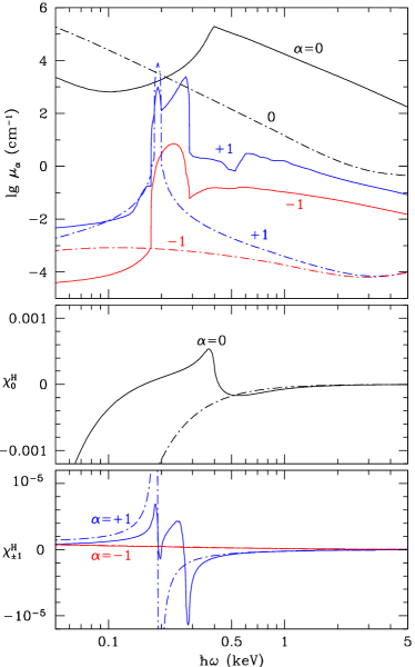
Fig. 7: Absorption coefficients (top panel) and polarizability coefficients $\chi^{\mathrm{H}}_{0}$ (middle panel) and $\chi^{\mathrm{H}}_{\pm 1}$ (bottom panel) in the partially ionized (solid curves) and fully ionized (dot-dashed curves) plasma models at $B=3\times 10^{13}$ G, $\rho=1$ g cm^-3 and $T=3.16\times 10^{5}$ K.

The anti-Hermitian part of the polarizability tensor determines the opacities: $\varkappa_{\alpha}(\omega)=4\pi\omega\chi^{\mathrm{A}}_{\alpha}(\omega)/(\rho c)$. Then the Kramers-Kronig relation gives [363, 364]

$$\chi^{\mathrm{H}}_{\alpha}(\omega) = \frac{c\rho}{4\pi^{2}\omega}\,\bigg{\{}\!\int_{0}^{\omega}\!\big{[}\,\varkappa_{\alpha}(\omega+\omega^{\prime})-\varkappa_{\alpha}(\omega-\omega^{\prime})\,\big{]}\frac{\mathrm{d}\omega^{\prime}}{\omega^{\prime}}$$ (74)

$$+ \int_{2\omega}^{\infty}\frac{\varkappa_{\alpha}(\omega^{\prime})}{\omega^{\prime}-\omega}\,\mathrm{d}\omega^{\prime}-\int_{0}^{\infty}\frac{\varkappa_{-\alpha}(\omega^{\prime})}{\omega^{\prime}+\omega}\,\mathrm{d}\omega^{\prime}\bigg{\}}.$$

Thus we can calculate the polarizability tensor $\bm{\chi}$ from the opacities $\varkappa_{\alpha}(\omega)$. It has been done in [363] for a gas of neutral hydrogen atoms and in [364] for partially ionized hydrogen plasmas.

Figure 7 shows the cyclic components of absorption coefficients, $\mu_{\alpha}=\rho\varkappa_{\alpha}$ in the top panel, and corresponding polarizability components $\chi^{\mathrm{H}}_{\alpha}$ in the middle and bottom panels, for a partially ionized hydrogen plasma at $B=3\times 10^{13}$ G, $\rho=1$ g cm^-3, and $T=3.16\times 10^{5}$ K. In this case, the neutral fraction is 89%. For comparison we show the results of an analogous calculation for the fully-ionized plasma model. In addition to the proton cyclotron resonance at $\hbar\omega=0.19$ keV that is present in both models, the absorption coefficients show rather pronounced features due to atomic transitions in the partially ionized plasma model. Most remarkable are the absorption features due to bound-bound transitions at $\hbar\omega\approx 0.2$–0.3 keV for $\mu_{+1}$ and the photoionization jump (partly smeared by the magnetic broadening) at $\hbar\omega=0.4$ keV for $\mu_{0}$. These features have clear imprints on the behavior of $\chi^{\mathrm{H}}_{+1}$ and $\chi^{\mathrm{H}}_{0}$.

6.3 Vacuum polarization

In certain ranges of density $\rho$ and frequency $\omega$, normal-mode properties are dramatically affected by a specific QED effect called vacuum polarization (its other manifestation has already been considered in § 5.5). The influence of the vacuum polarization on the neutron-star emission has been first evaluated in [365, 366] and studied in detail in the review [367]. If the vacuum polarization is weak, then it can be linearly added to the plasma polarization. Then the complex dielectric tensor can be written as $\bm{\varepsilon}^{\prime}=\mathbf{I}+4\pi\chi+4\pi\chi^{\mathrm{vac}},$ where

$$\bm{\chi}^{\mathrm{vac}}=(4\pi)^{-1}\,\mathrm{diag}(\bar{a},\bar{a},\bar{a}+\bar{q})$$ (75)

is the vacuum polarizability tensor, and diag(…) denotes the diagonal matrix. Magnetic susceptibility of vacuum is determined by expression

$$\bm{\mu}^{-1}=\mathbf{I}+\mathrm{diag}(\bar{a},\bar{a},\bar{a}+\bar{m}).$$ (76)

Adler [368] obtained the vacuum polarizability coefficients $\bar{a}$, $\bar{q}$, and $\bar{m}$ that enter Eqs. (75) and (76) in an explicit form at $b\ll 1$, Heyl and Hernquist [369] expressed them in terms of special functions in the limits of $b\ll 1$ and $b\gg 1$. Kohri and Yamada [370] presented their numerical calculations. Finally, in [364] we found simple but accurate expressions

$$\bar{a}=-\frac{2\alpha_{\mathrm{f}}}{9\pi}\ln\bigg{(}1+\frac{b^{2}}{5}\,\frac{1+0.25487\,b^{3/4}}{1+0.75\,b^{5/4}}\bigg{)},$$ (77)

$$\bar{q}=\frac{7\alpha_{\mathrm{f}}}{45\pi}\,b^{2}\,\frac{1+1.2\,b}{1+1.33\,b+0.56\,b^{2}},$$ (78)

$$\bar{m}=-\frac{\alpha_{\mathrm{f}}}{3\pi}\,\frac{b^{2}}{3.75+2.7\,b^{5/4}+b^{2}}.$$ (79)

The coefficients (77) – (79) are not small at $B\gtrsim 10^{16}$ G, therefore the vacuum refraction coefficients substantially differ from unity. In such strong fields, the vacuum that surrounds a neutron star acts as a lens, distorting its radiation [371, 372, 373]. At smaller $B$, the vacuum polarization results in a resonance, which manifests in the coincidence of the normal-mode polarization vectors at a certain frequency, depending on plasma density. In the photospheres with $B\gtrsim 10^{13}$ G, this resonance falls in the range $\sim 0.1$ – 1 keV and affects the thermal spectrum.

6.4 Polarization vectors of the normal modes

Shafranov [374] obtained the polarization vectors $\bm{e}_{j}$ for fully ionized plasmas. Ho and Lai [375] presented their convenient expressions in terms of the coefficients $\varepsilon_{\perp}$, $\varepsilon_{\|}$, $\varepsilon_{\wedge}$, $\bar{a}$, $\bar{q}$, and $\bar{m}$, including the contributions of electrons, ions, and vacuum polarization. In the Cartesian coordinate system ($xyz$) with the $z$-axis along the wave vector $\bm{k}$ and with $\bm{B}$ in the plane $x$–$z$, one has

$$\bm{e}_{j}=\left(\begin{array}[]{c}e^{j}_{x}\\ e^{j}_{y}\\ e^{j}_{z}\end{array}\right)=\frac{1}{\sqrt{1+K_{j}^{2}+K_{z,j}^{2}}}\,\left(\begin{array}[]{c}\mathrm{i}K_{j}\\ 1\\ \mathrm{i}K_{z,j}\end{array}\right),$$ (80)

where

$$K_{j}=\beta\left\{1+(-1)^{j}\left[1+\frac{1}{\beta^{2}}+\frac{\bar{m}}{1+\bar{a}}\frac{\sin^{2}\theta_{B}}{\beta^{2}}\right]^{1/2}\right\},\hskip 20.00003pt$$ (81)

$$K_{z,j}=-\frac{(\varepsilon_{\perp}^{\prime}-\varepsilon_{\|}^{\prime})K_{j}\cos\theta_{B}+\varepsilon_{\wedge}}{\varepsilon_{\perp}^{\prime}\sin^{2}\theta_{B}+\varepsilon_{\|}^{\prime}\cos^{2}\theta_{B}}\,\sin\theta_{B},\hskip 20.00003pt$$ (82)

$$\beta=\frac{\varepsilon_{\|}^{\prime}-\varepsilon_{\perp}^{\prime}+\varepsilon_{\wedge}^{2}/\varepsilon_{\perp}^{\prime}+\varepsilon_{\|}^{\prime}\,\bar{m}/(1+\bar{a})}{2\,\varepsilon_{\wedge}}\,\,\frac{\varepsilon_{\perp}^{\prime}}{\varepsilon_{\|}^{\prime}}\,\,\frac{\sin^{2}\theta_{B}}{\cos\theta_{B}},\hskip 20.00003pt$$ (83)

$\varepsilon_{\perp}^{\prime}=\varepsilon_{\perp}+\bar{a}$, and $\varepsilon_{\|}^{\prime}=\varepsilon_{\|}+\bar{a}+\bar{q}$. If the plasma and vacuum polarizabilities are small ($|\chi^{\mathrm{H}}_{\alpha}|\ll(4\pi)^{-1}$ and $|\bar{a}|,\bar{q},|\bar{m}|\ll 1$), as usual,

$$\beta\approx\frac{2\chi^{\mathrm{H}}_{0}-\chi^{\mathrm{H}}_{+1}-\chi^{\mathrm{H}}_{-1}+(\bar{q}+\bar{m})/(2\pi)}{2\,(\chi^{\mathrm{H}}_{+1}-\chi^{\mathrm{H}}_{-1})}\,\frac{\sin^{2}\theta_{B}}{\cos\theta_{B}}.$$ (84)

6.5 Opacities

In the approximation of isotropic scattering, at a given frequency $\omega$, the opacities can be presented in the form

$$\varkappa_{j}^{\mathrm{a}}=\sum_{\alpha=-1}^{1}|e_{j,\alpha}(\theta_{B})|^{2}\,\frac{\sigma_{\alpha}^{\mathrm{a}}}{m_{\mathrm{i}}},$$ (85)

$$\varkappa_{jj^{\prime}}^{\mathrm{s}}\!=\!\!{\frac{3}{4}}\!\!\sum_{\alpha=-1}^{1}\!\!|e_{j,\alpha}(\theta_{B})|^{2}\,\frac{\sigma_{\alpha}^{\mathrm{s}}}{m_{\mathrm{i}}}\int_{0}^{\pi}\!\!\!|e_{j^{\prime},\alpha}(\theta_{B}^{\prime})|^{2}\sin\theta_{B}^{\prime}\,\mathrm{d}\theta_{B}^{\prime},$$ (86)

where $\sigma_{\alpha}$ are the cross sections for the three basic polarizations according to Eq. (43). The partial cross sections $\sigma_{\alpha}^{\mathrm{a,s}}$ include contributions of photon interaction with free electrons or ions (free-free transitions) as well as with bound states of atoms and ions (bound-bound and bound-free transitions). The latter implies, in particular, averaging of the cross sections of photon and atom absorption over all values of $K_{\perp}$. Since the distribution over $K_{\perp}$ is continuous for the atoms and discrete for the ions, such averaging for atoms reduces to an integration over $K_{\perp}$, analogous to Eq. (61), whereas for ions it implies summation with an appropriate statistical weight. To date, such calculation has been realized for atoms of hydrogen [266, 350] and helium [308].

Figure 8 presents opacities for the two normal modes propagating at the angle $\theta_{B}=10^{\circ}$ to the magnetic field under the same physical conditions as in Fig. 7. One can clearly distinguish the features reflecting the peaks at the ion cyclotron frequency and the resonant atomic frequencies, and the line crossings related to the behavior of the plasma polarizability as function of frequency. For comparison, we show also opacities for the fully ionized plasma model under the same conditions. They miss the features related to the atomic resonances, and their values is underestimated by orders of magnitude in a wide frequency range.

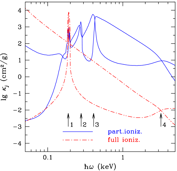
Fig. 8: Logarithm of spectral opacities ($\log\varkappa_{j}$) for two normal modes, propagating at the angle $\theta_{B}=10^{\circ}$ to the magnetic field lines in a hydrogen plasma at $B=3\times 10^{13}$ G, $T=3.16\times 10^{5}$ K, $\rho=1$ g cm^-3. Solid curves: partially ionized plasma model; dot-dashed curves: fully-ionized plasma model. The lower (upper) curve of each type corresponds to the extraordinary (ordinary) wave. The arrows indicate the features at resonant frequencies: 1– the ion cyclotron resonance $\omega=\omega_{\mathrm{ci}}$; 2 – energy threshold for a transition between the lowest two levels $\hbar\omega=|E_{0,0}^{(0)}-E_{1,0}^{(0)}|$; 3 – the ground-state binding energy $\hbar\omega=|E_{0,0}^{(0)}|$; 4 – the vacuum resonance.

6.6 Spectra of magnetic photospheres

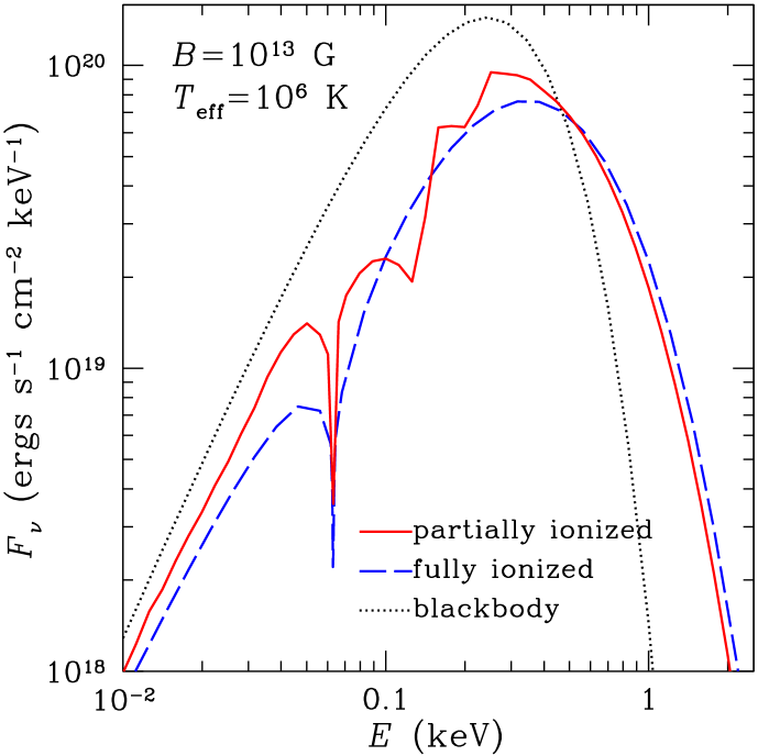
Fig. 9: Local spectrum of hydrogen photosphere with $B=10^{13}$ G (the field is normal to the surface) and $T_{\mathrm{eff}}=10^{6}$ K. The solid line presents a self-consistent model of a partially ionized photosphere, the dashed line presents the fully-ionized atmosphere model, and the dots show the blackbody spectrum. (The figure is provided by W. C. G. Ho.)

Shibanov and coworkers [376] were the first to perform detailed calculations of the spectra of radiation formed in the strongly magnetized neutron-star photospheres, using the fully ionized plasma model, and created a database of magnetic hydrogen spectra [269]. They have shown that the spectra of magnetic hydrogen and helium atmospheres are softer than the respective nonmagnetic spectra, but harder than the blackbody spectrum with the same temperature. In addition to the spectral energy distribution, these authors have also studied the polar diagram and polarization of the outgoing emission, which proved to be quite nontrivial because of redistribution of energy between the normal modes. The thermal radiation of a magnetized photosphere is strongly polarized, and the polarization sharply changes at the cyclotron resonance with increasing frequency. At contrast to the isotropic blackbody radiation, radiation of a magnetic photosphere consists of a narrow ($<5^{\circ}$) pencil beam along the magnetic field and a broad fan beam with typical angles $\sim 20^{\circ}-60^{\circ}$ [377] (see also [378]). These calculations have thus fully confirmed the early analysis by Gnedin and Sunyaev [11].

Later, analogous calculations were performed by other research groups [379, 375, 378]. They paid special attention to manifestations of the ion cyclotron resonance in observed spectra in the presence of superstrong magnetic fields, which was prompted by tentative magnetar discoveries. It was shown in [380] that the vacuum polarization leads in the superstrong fields to a conversion of the normal modes, when a photon related to one mode transforms, with certain probability, into a photon of the other mode while crossing a surface with a certain critical density. The latter density is related to the photon energy as

$$\rho=0.00964\,(A/Z)\,(\hbar\omega/\mbox{keV})^{2}\,B_{12}^{2}/f_{B}^{2}~{}\mbox{g~{}cm${}^{-3}$},$$ (87)

where $f_{B}^{2}=\alpha_{\mathrm{f}}b^{2}/[15\pi(\bar{q}+\bar{m})]$, while $\bar{q}$ and $\bar{m}$ are given by Eqs. (78), (79); $f_{B}$ weakly depends on $B$, and $f_{B}\approx 1$ at $B\lesssim 10^{14}$ G. The energy $\hbar\omega$ in Eq. (87) corresponds to the line crossing in Fig. 8, indicated by arrow 4. It follows from Eq. (87) that in the field of $B\sim 10^{14}$ G this energy coincides with the ion cyclotron energy at the density where the atmosphere is optically thin for the extraordinary mode, but optically thick for the ordinary mode. Under such conditions, the mode conversion strongly suppresses the ion cyclotron feature in the emission spectrum.

In the first computations of partially ionized photospheres of neutron stars with magnetic fields $B\sim 10^{12}$ – $10^{13}$ G that were presented in [346] and [339], the properties of the atoms in magnetic fields were calculated by the adiabatic Hartree-Fock method (§ 5.3). The atomic motion was either ignored [346], or treated approximately by the perturbation theory [339].

In [364], a hydrogen photosphere model has been constructed beyond the framework of the adiabatic approximation, taking the full account of the partial ionization as well as the atomic motion effects in the strong magnetic fields. Figure 9 gives an example of radiation spectrum going out of such photosphere with $B=10^{13}$ G. We see a narrow absorption line at the proton cyclotron energy $E=0.063$ keV and the features at higher energies, related to atomic transitions. For comparison, a spectrum calculated in the fully-ionized plasma model and the Planck spectrum are shown. The comparison shows that the two photospheric models have similar spectral shapes, but the model that allows for the partial ionization has additional features. The spectral maximum of both models is shifted to higher energies relative to the Planck maximum. This demonstrates that an attempt of interpretation of the hydrogen spectra with the blackbody model would strongly overestimate the effective temperature, while the fully-ionized photosphere model yields a more realistic temperature, but does not reproduce the spectral features caused by atomic transitions.

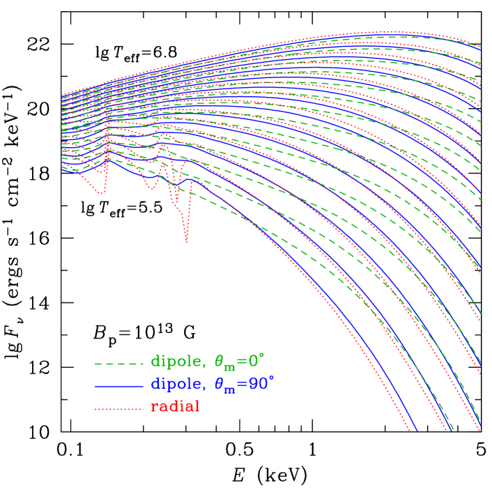
Fig. 10: Integral spectra of a hydrogen atmosphere of a neutron star with $M=1.4\,M_{\odot}$, $R=12$ km, and with different effective temperatures $T_{\mathrm{eff}}$ ($\log T_{\mathrm{eff}}$ (K) from 5.5 to 6.8 with step 0.1). The dashed and solid lines represent the model with a dipole field of strength $B_{\mathrm{p}}=10^{13}$ G at the pole and oriented along and across the line of sight, respectively. For comparison, the dotted curve shows the model with a constant field $B=10^{13}$ G, normal to the surface.

Magnetic fields and temperatures of neutron stars vary from one surface point to another. In order to reproduce the radiation spectrum that comes to an observer, one can use Eq. (15). The problem is complicated, because the surface distributions of the magnetic field and the temperature are not known in advance. As a fiducial model one conventionally employs the relativistic dipole model (16), (17), while the temperature distribution, consistent with the magnetic-field distribution, is found from calculations of heat transport in neutron-star envelopes (e.g., [84]). Results of such calculations, performed in [381], are shown in Fig. 10. We see that the spectral features are strongly smeared by the averaging over the surface, and the spectrum depends on the magnetic axis orientation $\theta_{\mathrm{m}}$. When the star rotates, the latter dependence leads to pulsations of the measured spectrum.

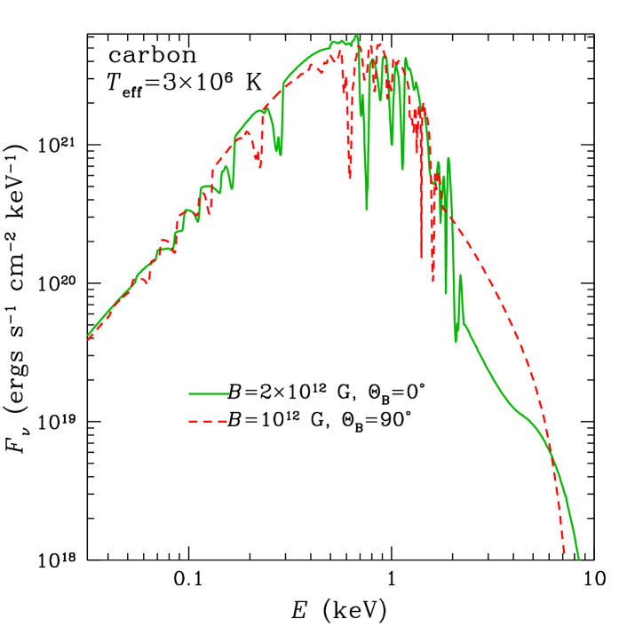
Fig. 11: Local spectra at the magnetic pole (solid curve) and equator (dashed curve) for a neutron star with carbon atmosphere, the dipole field with polar strength of $B_{\mathrm{p}}=2\times 10^{12}$ G (neglecting the relativistic corrections) and uniform effective temperature $3\times 10^{6}$ K. (Fig. 20 from [348], reproduced with permission of the authors and © Oxford University Press.)

Mori et al. [347, 348] calculated model spectra of neutron-star photospheres composed of the atoms and ions of elements with $Z_{\mathrm{n}}\lesssim 10$. They calculated the quantum-mechanical properties of the atoms and ions by the method of Mori and Hailey [301] and treated the atomic motion effects by the perturbation theory (§ 5.6). The equation of state and ionization equilibrium were determined by the methods described in § 5.8, the plasma polarizability was calculated by Eq. (74), and the opacities were treated according to § 6.5. As an example, Fig. 11 demonstrates local spectra of the carbon photosphere with magnetic field $B=2\times 10^{12}$ G, normal to the surface, and the field $B=10^{12}$ G parallel to the surface, which approximately (with account of neither relativistic corrections nor temperature nonuniformity) corresponds to the local spectra at the magnetic pole and equator of a star with a dipole magnetic field. By analogy to the case of hydrogen photosphere, the integration over the surface between the pole and equator should smear the spectral features between the two limiting curves shown in the figure.

The results described in this section have been used to produce databases of spectra of partially ionized, strongly magnetized neutron-star photospheres composed of hydrogen [381] and heavier elements up to neon [348].

7 Spectra of neutron stars with condensed surfaces

7.1 Radiation of a naked neutron star

As we have seen in § 5.10, the stars with a very low effective temperature and a superstrong magnetic field can have a liquid or solid condensed surface. In this case, thermal emission can escape directly from the metallic surface without transformation in a gaseous atmosphere, and then the spectrum is determined by the emission properties of this surface. Formation of thermal spectra at a condensed surface of a strongly magnetized neutron star depends on its reflection properties, which were considered in [383, 384, 385, 115, 386, 387, 388]. The first works [383, 384] gave order-of-magnitude estimates. A method of detailed calculation of the reflectivity was proposed in [385] and then was used with some modifications in [385, 115, 386, 387, 388]. It is as follows. First, the normal-mode polarization vectors $\bm{e}_{1,2}^{\mathrm{(t)}}$ in the medium under the surface, Eqs. (80) – (82), and the complex refraction coefficients are expressed as functions of the angles $\theta_{k}$ and $\varphi_{k}$ that determine the direction of a reflected ray (Fig. 1), using the standard dispersion equation for the transmitted wave and the Snell’s law. Second, the complex electric amplitudes of the incident, reflected, and transmitted waves are expanded over the respective basic polarization vectors $\bm{e}_{1,2}^{\mathrm{(i,r,t)}}$. Then the Maxwell boundary conditions yield a system of equations, which determine the coefficients of these expansions. These reflected-wave expansion coefficients form the reflection matrix $\{r_{jj^{\prime}}\}$ and determine the surface reflectivity for each incident-wave polarization, $r_{\omega,j}=\sum_{j^{\prime}}r_{\omega,jj^{\prime}}$. Then the total emissivity $\varepsilon_{\omega}=1-\frac{1}{2}(r_{\omega,1}+r_{\omega,2})$.

The early works assumed that the ions are firmly fixed at the crystalline lattice sites in the metal. In [386, 387, 388] the authors have considered not only this model, but also the opposite limit of free ions. It is assumed [386] that the real reflectivity of the surface lies between the limits given by these two models, although this problem has not yet been definitely solved.

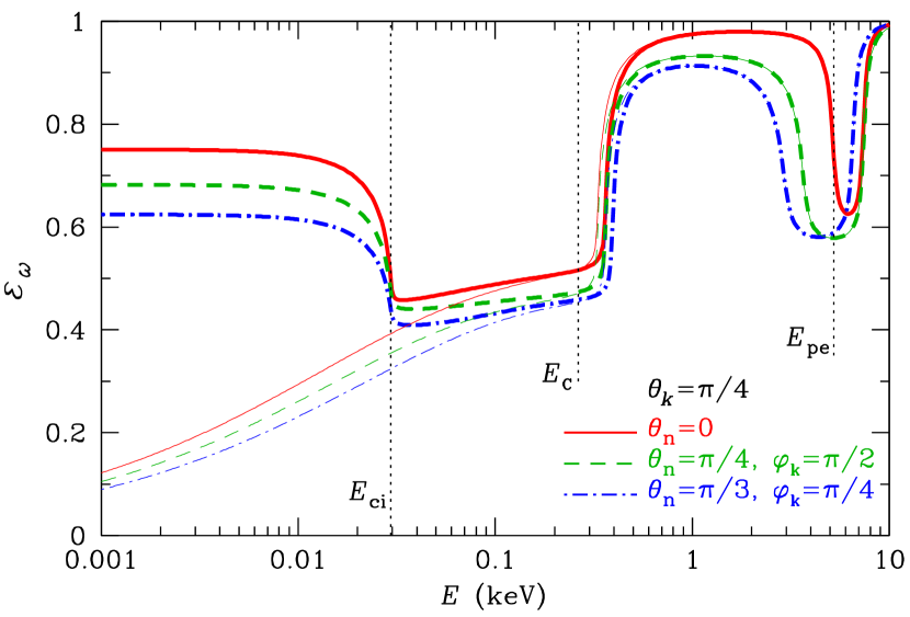
Fig. 12: Emissivity of a condensed iron surface at $B=10^{13}$ G and $T=10^{6}$ K, averaged over polarizations, is shown as a function of energy of a photon emitted at the angle $\theta_{k}=45^{\circ}$, for different magnetic-field inclination angles $\theta_{\mathrm{n}}$ and azimuthal angles $\varphi_{k}$. The thick and thin curves are obtained, respectively, in the models of free and fixed ions. Vertical dotted lines mark positions of the characteristic energies: the ion cyclotron energy $E_{\mathrm{ci}}=\hbar\omega_{\mathrm{ci}}$, the electron plasma energy $E_{\mathrm{pe}}=\hbar\omega_{\mathrm{pe}}$, and the hybrid energy $E_{\mathrm{C}}$.

Figure 12 shows examples of the emissivity $\varepsilon_{\omega}$, normalized to the blackbody emissivity, as a function of photon energy $E=\hbar\omega$, according to the free- and fixed-ions models, for different values of the angles $\theta_{\mathrm{n}}$, $\theta_{k}$, and $\varphi_{k}$ that are defined in Fig. 1. The characteristic energies $E_{\mathrm{ci}}=\hbar\omega_{\mathrm{ci}}$, $E_{\mathrm{pe}}=\hbar\omega_{\mathrm{pe}}$, and $E_{\mathrm{C}}=E_{\mathrm{ci}}+E_{\mathrm{pe}}^{2}/\hbar\omega_{\mathrm{c}}$ are marked. The spectral features near these energies are explained in [386]. For instance, the emissivity suppression at $E_{\mathrm{ci}}\lesssim E\lesssim E_{\mathrm{C}}$ is due to the strong damping of one of the two normal modes in the plasma in this energy range. In the fixed-ions mode, $\omega_{\mathrm{ci}}\to 0$, therefore there is no kink of the spectrum at $E\approx E_{\mathrm{ci}}$ in this model. The results almost coincide in the two alternative models at $E\gg E_{\mathrm{ci}}$, but strongly differ at $E\lesssim E_{\mathrm{ci}}$, which may be important for magnetar spectra. Near the electron plasma energy $E_{\mathrm{pe}}=\hbar\omega_{\mathrm{pe}}$, there is a resonant absorption, depending on the directions of the incident wave and the magnetic field.

The local flux density of radiation from a condensed surface is equal to the Planck function $\mathcal{B}_{\omega,T}$ (18), multiplied by the normalized emissivity $\varepsilon_{\omega}$. Since $\varepsilon_{\omega}$ depends on the frequency $\omega$ and on the angles $\theta_{\mathrm{n}}$, $\theta_{k}$, and $\varphi_{k}$ (Fig. 1), thermal radiation depends on the frequency and angles in a nontrivial way. In Fig. 12, the emissivity is averaged over polarizations. But $r_{\omega,1}\neq r_{\omega,2}$, hence the thermal emission of a condensed surface is polarized, the polarization depending in an equally nontrivial way on the frequency and angles. For example, the degree of linear polarization can reach tens percent near the frequencies $\omega_{\mathrm{ci}}$ and $\omega_{\mathrm{pe}}$, which makes promising the polarization diagnostics of neutron stars with condensed surfaces. Both the intensity and the polarization degree can be evaluated using analytical expressions, which have been constructed in [388] for the reflectivity matrix of a condensed iron surface for $B=10^{12}$ – $10^{14}$ G.

7.2 Thin and layered atmospheres

Motch, Zavlin, and Haberl [389] suggested that some neutron stars can possess a hydrogen atmosphere of a finite thickness above the solid iron surface. If the optical depth of such atmosphere is small for some wavelengths and large for other ones, this should lead to a peculiar spectrum, different from the spectra of thick atmospheres. Such spectra were calculated in [390, 391, 392] using simplified boundary conditions for the radiative transfer equation at the inner boundary of the atmosphere. More accurate boundary conditions have been suggested in [388], where the authors have taken into account that an extraordinary or ordinary wave, falling from outside on the interface, gives rise to reflected waves of both polarizations, whose intensities add to the respective intensities of the waves emitted by the condensed surface:

$$I_{\omega,j}(\theta_{k},\varphi) = \sum_{j^{\prime}=1,2}r_{\omega,jj^{\prime}}(\theta_{k},\varphi)\,I_{\omega,j^{\prime}}(\pi-\theta_{k},\varphi)$$ (88)

$$+\textstyle\frac{1}{2}\big{[}1-r_{\omega,j}(\theta_{k},\varphi)\big{]}\,\mathcal{B}_{\omega,T}.$$

In Ref. [388], the reflectivity matrix was calculated and fitted for linear polarizations, and then converted into the reflectivity matrix $\{r_{\omega,jj^{\prime}}\}$ for normal modes pertinent to Eq. (88), using an approximate relation valid for a sufficiently rarefied photosphere.

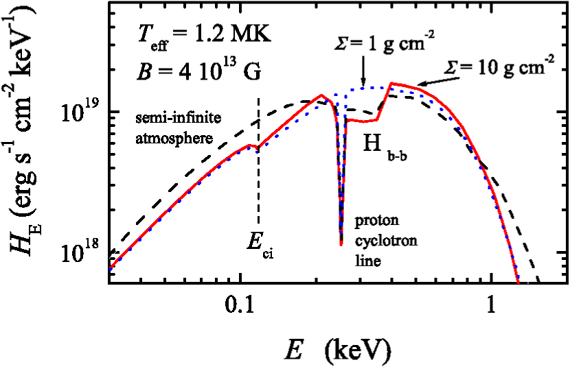
Fig. 13: Comparison of the radiation spectrum of a neutron star with a partially ionized thick hydrogen photosphere (dashed line) with the spectra that are formed at hydrogen column densities of 1 g cm^-2 (dots) and 10 g cm^-2 (solid line) over the iron surface of the star (Fig. 12 from [388], provided by V. F. Suleimanov, reproduced with permission of the author and ©ESO.)

In Fig. 13 we show local spectra of radiation emitted by hydrogen atmospheres of different thicknesses over the iron neutron-star surface with the magnetic field $B=4\times 10^{13}$ G, normal to the surface with effective temperature $T_{\mathrm{s}}=1.2\times 10^{6}$ K. The narrow absorption line corresponds to the proton cyclotron resonance in the atmosphere. The feature to the right of it is related to atomic transitions (H_b-b). It has a large width because of the motion effects (§ 5.6). This feature is formed mainly at depths $\sim 2$ g cm^-2, that is why it is almost invisible in the spectrum of the thinnest atmosphere that has the column density of 1 g cm^-2. The kink at $E_{\mathrm{ci}}=0.12$ keV corresponds to the ion cyclotron energy of iron, therefore it is absent for the pure hydrogen atmosphere. The spectrum of the moderately deep atmosphere (10 g cm^-2) reveals all the three features. At high energies ($E\gtrsim 1$ keV), the spectrum is determined by the condensed-surface emission, because both finite atmospheres are almost transparent at such energies. The spectrum of the pure hydrogen atmosphere is harder in this spectral range (cf. § 6.6).

The origin of the thin atmospheres remains hazy. Ho et al. [390] discussed three possible scenarios. First, it is the accretion from the interstellar medium. But its rate should be very low, in order to accumulate the hydrogen mass $4\pi R^{2}y_{\mathrm{col}}\sim 10^{-20}M_{\odot}$ in $\sim 10^{6}$ years. Another scenario assumes diffusive nuclear burning of a hydrogen layer, fell back soon after the formation of the neutron star [112]. But this process is too fast at the early cooling epoch, when the star is relatively hot, and would have rapidly consumed all the hydrogen on the surface [393]. The third possibility is a self-regulating mechanism that is driven by nuclear spallation in collisions with ultrarelativistic particles at the regions of open field lines, which leads to creation of protons and alpha-particles. The estimate (23) for the penetration depth of the magnetospheric accelerated particles indicates that this process could create a hydrogen layer of the necessary thickness $y_{\mathrm{col}}\sim 1$ g cm^-2.

It is natural to consider also an atmosphere having a helium layer beneath the hydrogen layer. Indeed, all three scenarios assume that a hydrogen-helium mixture appears originally at the surface, and the strong gravity quickly separates these two elements. Such “sandwich atmosphere” was considered in [391], where the authors showed that its spectrum can have two or three absorption lines in the range $E\sim(0.2$ – 1) keV at $B\sim 10^{14}$ G.

8 Theoretical interpretation of observed spectra

As we have seen in § 4, theoretical models of nonmagnetic atmospheres are successfully applied to analyses of spectra of many neutron stars with relatively weak magnetic fields $B\lesssim 10^{9}$ G. There are only a few such examples for the stars with strong magnetic fields. They will be discussed in this section. At the end of the section we will give a general compilation of modern estimates of masses and radii of neutron stars with weak and strong magnetic fields, based on the photosphere models.

8.1 RX J1856.5–3754

As we discussed in § 4.4, there is no satisfactory description of the spectrum of the “Walter star” RX J1856.5–3754 based on nonmagnetic atmosphere models. Simple models of magnetic atmospheres also failed to solve this problem. It was necessary to explain simultaneously the form of the spectrum in the X-ray and optical ranges that reveal substantially different color temperatures $T_{\mathrm{bb}}^{\infty}$, along with the complete absence of absorption lines or other spectral features that was confirmed at a high significance level. To solve this problem, Ho [390, 394] involved the model of a partially ionized hydrogen atmosphere of finite thickness above a condensed iron surface with a strong magnetic field. He managed to reproduce the measured spectrum of RX J1856.5–3754 in the entire range from X-rays to optical within observational errorbars. The best agreement between the theoretical and observed spectra has been achieved at the atmosphere column density $y_{\mathrm{col}}=1.2$ g cm^-2, $B\sim(3$ – $4)\times 10^{12}$ G, $T_{\mathrm{eff}}^{\infty}=(4.34\pm 0.03)\times 10^{5}$ K, $z_{g}=0.25\pm 0.05$, and $R_{\infty}=17.2^{+0.5}_{-0.1}\,D_{140}$ km. Here, the errors are given at the $1\sigma$ significance level, and $D_{140}\equiv D/(140$ pc). Note that a fit of the observed X-ray spectrum with the Planck function yields a 70% higher temperature and a 3.5 times smaller radius of the emitting surface. Such huge difference exposes the importance of a correct physical interpretation of an observed spectrum for evaluation of neutron-star parameters.

With the aid of expressions (6) – (8) and Eq. (3), we obtain from these estimates $T_{\mathrm{eff}}=(5.4\pm 1.1)\times 10^{5}$ K, $R=13.8^{+0.9}_{-0.6}\,D_{140}$ km, and $M=1.68^{+0.22}_{-0.15}\,D_{140}\,M_{\odot}$. Forgetting for a moment the factor $D_{140}$, one might conclude that this radius is too large for such mass. However, the distance to the star is not very accurately known. The value $D=140$ pc was adopted in [390] from [395] and lies between alternative estimates $D\approx 117$ pc [396] and $D\approx(160$ – 170) pc [397, 398]. More recently, a more accurate estimate of the distance was obtained, $D=123^{+11}_{-15}$ pc [399]. With the latter estimate, we obtain $R=12.1^{+1.3}_{-1.6}$ km and $M=1.48^{+0.16}_{-0.19}\,M_{\odot}$, which removes all the contradictions. Nevertheless, the given interpretation of the spectrum is not indisputable, since it does not agree with the magnetic-field estimate $B\approx 1.5\times 10^{13}$ G that has been obtained for this star from Eq. (1) in [400].

Using the same thin-atmosphere model, Ho [394] analyzed the light curve of RX J1856.5–3754 and obtained constraints on the angles $\alpha$ and $\zeta$ (Fig. 1). It turned out that the light curve can be explained if one of these angles is small ($<6^{\circ}$), while the other angle lies between $20^{\circ}$ and $45^{\circ}$. In this case, the radio emission around the magnetic poles does not cross the line of sight. As noted in [394], this may explain the non-detection of this star as a radio pulsar [165].

8.2 RBS 1223

Hambaryan et al. [401] analyzed the spectrum of the X-ray source RBS 1223, by a method analogous to the case of RX J1856.5–3754 described in § 8.1. RBS 1223 reveals a complex structure of the X-ray spectrum, which can be described by a wide absorption line centered around $\hbar\omega=0.3$ keV, superposed on the Planck spectrum, with the line parameters depending on the stellar rotation phase. Using all 2003 – 2007 XMM-Newton observations of this star, the authors [401] obtained a set of X-ray spectra for different rotation phases. They tried to interpret these spectra with different models, assuming magnetic fields $B\sim 10^{13}$ – $10^{14}$ G, different atmosphere compositions, possible presence of a condensed surface and a finite atmosphere. Different surface temperature distributions were described by a self-consistent parametric model of Ref. [46].

As a result, the authors [401] managed to describe the observed spectrum and its rotational phase dependence with the use of the model of the iron surface covered by partially ionized hydrogen atmosphere with $y_{\mathrm{col}}\sim 1$ – 10 g cm^-2, with mutually consistent asymmetric bipolar distributions of the magnetic field and the temperature, with the polar values $B_{\textrm{p1}}=B_{\textrm{p2}}=(0.86\pm 0.02)\times 10^{14}$ G, $T_{\mathrm{p1}}=1.22^{+0.02}_{-0.05}$ MK, and $T_{\mathrm{p2}}=1.15\pm 0.04$ MK. The magnetic field and temperature proved to be rather smoothly distributed over the surface. When compared to the theoretical model [46], it implies the absence of a superstrong toroidal component of the crustal magnetic field. The integral effective temperature is $T_{\mathrm{eff}}\approx 0.7$ MK. The gravitational redshift is estimated to be $z_{g}=0.16^{+0.03}_{-0.01}$, which converts into $(M/M_{\odot})/R_{6}=0.87^{+0.13}_{0.05}$ and suggests a stiff EOS of the neutron-star matter.

We must note that the paper [401] preceded the work [388], which was discussed in § 7. For this reason, the authors of [401] used rough approximations for the iron-surface emissivity, published before, and simplified boundary conditions for the radiative transfer equations. An analysis of the same spectra with the use of the improved results for the emissivity and more accurate boundary conditions, described in § 7, remains to be done in the future.

Table 1: Estimates of neutron-star masses and radii based on atmosphere models.

Object	$R$ (km)	$M$ ($M_{\odot}$)	$D$ (kpc)	Ref.	Notes
qLMXB X7 in 47 Tuc	$14.5^{+1.8}_{-1.6}$	$1.4$ [a]	4.85 [a]	[209]	[b]
qLMXB XTE 1701–462	$10.5\pm 2.5$ [c]	1.4 [a]	8.8 [a]	[136]	[b]
qLMXB EXO 0748–676	$13.7^{+1.0}_{-2.7}$	$1.8^{+0.4}_{-0.6}$	7.1 [a]	[134]	[b]
same object	$11.8^{+0.7}_{-2.2}-15.2^{+1.5}_{-3.0}$	$1.5^{+0.5}_{-0.5}-2.1^{+0.4}_{-0.8}$	$5.9-8.3$	[134]	[d], [e]
qLMXB in M28	$10.5^{+2.0}_{-2.9}$	$1.25^{+0.54}_{-0.63}$	$5.5$ [a]	[242]	[b]
same object	$9^{+3}_{-3*}$	$1.4^{+0.4}_{-0.9*}$	$5.5$ [a]	[243]	[b]
same object	$14^{+3}_{-8*}$	$2.0^{+0.5}_{-1.5*}$	$5.5$ [a]	[243]	[e]
qLMXB in NGC 6397	$6.6^{+1.2}_{-1.1}$	$0.84^{+0.30}_{-0.28}$	$2.02$ [a]	[242]	[b]
qLMXB in M13	$10.1^{+3.7}_{-2.8}$	$1.27^{+0.71}_{-0.63}$	$6.5$ [a]	[242]	[b]
same object	$10.6^{+2.1}_{-2.2}$	1.4 [a]	7.7 [a]	[244]	[b]
same object	$14.6^{+3.5}_{-3.1}$	1.4 [a]	7.7 [a]	[244]	[e]
qLMXB in $\omega$ Cen	$20.1^{+7.4}_{-7.2}$	$1.8^{+1.0}_{-1.1}$	$4.8$ [a]	[242]	[b]
qLMXB in NGC 6304	$9.6^{+4.9}_{-3.4}$	$1.16^{+0.90}_{-0.56*}$	$6.22$ [a]	[242]	[b]
CCO in Cas A	$15.6^{+1.3}_{-2.7}$	$1.4$ [a]	3.4 [a]	[214]	[f]
same object	$8-17$	$1.5-2.4$	$3.3-3.7$	[214]	[d], [f]
CCO in HESS J1731	$12.6^{+2.1}_{-5.3}-15.6^{+3.6}_{-5.3}$	$1.5^{+0.4}_{-0.6}-2.2^{+0.3}_{-0.9}$	$3.2-4.5$	[237]	[d], [f]
Burster 4U 1724–307	$14.7\pm 0.8$	$1.9\pm 0.4$	5.3–7.7	[151]	[b]
same object	$18\pm 3.5$	$1.05^{+0.55}_{-0.4}$	5.3–7.7	[151]	[e]
Burster GS 1826–24	$<8.2$	$<1.3$	$<4.3$ [g]	[219]	[b]
same object	$<19.8$	$<2.8$	$<9.7$ [g]	[219]	[e]
PSR J0437–4715	$>11.1$ ($3\sigma$)	1.76 [a]	0.1563 [a]	[252]	[b]; see § 4.6
XDINS RX J1856	$12.1^{+1.3}_{-1.6}$	$1.48^{+0.16}_{-0.19}$	$0.123^{+0.011}_{-0.015}$ [h]	[390]	[c], [i], [j]; see § 8.1
XDINS RBS 1223	$16^{+1}_{-2}$	1.4 [a]	$0.380^{+0.015}_{-0.030}$	[401]	[c], [i], [k]; see § 8.2

Notes: Errors are listed at significance level 90%, unless otherwise stated. The asterisk at a value of an error signifies that a hard limit of a model was reached. [a] The parameter is fixed. [b] Nonmagnetic H atmosphere. [c] Errors at the significance level $1\sigma$ (68%). [d] Results for selected limiting $D$ from a range of possible values. [e] Nonmagnetic He atmosphere. [f] Nonmagnetic C atmosphere. [g] Constraint on $D\xi_{\mathrm{b}}^{1/2}$ is given, where $\xi_{\mathrm{b}}$ is the anisotropy factor. [h] $D$ is adopted from [399]. [i] Partially ionized thin H atmosphere over iron surface. [j] $y_{\mathrm{col}}=1.2$ g cm^-2, $B\sim(3$ – $4)\times 10^{12}$ G. [k] $y_{\mathrm{col}}\sim 1$ g cm^-2, mutually consistent distributions of magnetic field $B\sim 8\times 10^{13}$ G and temperature $T_{\mathrm{s}}\sim 0.7$ MK.

8.3 1E 1207.4–5209

The discovery of absorption lines in the spectrum of CCO 1E 1207.4–5209 at energies $E\sim 0.7\,N$ keV ($N=1,2,\ldots$) immediately entrained the natural assumption that they are caused by cyclotron harmonics [172]. As we have seen in § 5.2, such harmonics can be only electronic, as the ion harmonics are unobservable. Therefore, this interpretation implies $B\approx 7\times 10^{10}$ G. Mori et al. [173] showed that only the first and second lines in the spectrum of 1E 1207.4–5209 are statistically significant, but some authors take also the third and fourth lines into account. This hypothesis was developed in [264], where the authors include in the treatment both types of the electron cyclotron harmonics that were discussed in § 5.2: the quantum oscillations of the Gaunt factor and the relativistic thermal harmonics. It is possible that the analogous explanation of the shape of the spectrum may be applied also to CCO PSR J0821–4300 [167].

Mori et al. [347, 348] have critically analyzed the earlier hypotheses about the origin of the absorption lines in the spectrum of 1E 1207.4–5209 and suggested their own explanation. They analyzed and rejected such interpretations as the lines of molecular hydrogen ions, helium ions, and also as the cyclotron lines and their harmonics. One of the arguments against the latter interpretation is that the fundamental cyclotron line should have much larger depth in the atmosphere spectrum than actually observed. Another argument is that the cyclotron lines and harmonics have small widths at a fixed $B$, therefore their observed width in the integral spectrum is determined by the $B$ distribution. Thus their width should be the same, in contradiction to observations [347]. These arguments were neglected in [264]. It has to be noted that in [347], as well as in [264], the authors studied the cyclotron harmonics in spectra of fully ionized plasmas. The effect of the partial ionization on the model spectrum remains unexplored.

As an alternative, Mori et al. [347, 348] suggested models of atmospheres composed of mid-$Z$ elements. An example of such spectrum is shown in Fig. 11. Its convolution with the telescope point-spread function smears the line groups, producing wide and shallow suppressions of the spectral flux, similar to the observed ones. Integration of the local spectrum over the stellar surface, whose necessity we mentioned in § 6.6, should lead to an additional smearing of the spectral features. The authors [348] found that an oxygen atmosphere with magnetic field $B=10^{12}$ G provides a spectrum similar to the observed one. However, the constraint $B<3.3\times 10^{11}$ G that was obtained in [166] disagrees with this model, but rather favors the cyclotron interpretation of the lines.

Unlike the cases of RX J1856.5–3754 and RBS 1223 that were considered above, there is no published results of a detailed fitting of the observed spectrum of 1E 1207.4–5209 with a theoretical model. Thus the applicability of any of them remains hypothetical.

8.4 PSR J1119–6127

Recently, the partially ionized, strongly magnetized hydrogen photosphere model [381] has been successfully applied to interpret the observations of pulsar J1119–6127 [146], for which the estimate (1) gives an atypically high field $B=4\times 10^{13}$ G. In the X-ray range, it emits pulsed radiation, which has apparently mostly thermal nature. At fixed $D=8.4$ kpc and $R=13$, the bolometric flux gives an estimate of the mean effective temperature $T_{\mathrm{eff}}\approx 1.1$ MK. It was difficult to explain, however, the large pulsed fraction ($48\pm 12$%) by the thermal emission. The authors [146] managed to reproduce the X-ray light curve of this pulsar assuming that one of its magnetic poles is surrounded by a heated area, which occupies 1/3 of the surface, is covered by hydrogen and heated to $1.5$ MK, while the temperature of the opposite polar cap is below $0.9$ MK.

8.5 Masses and radii: the results

Table 1 presents modern estimates of neutron-star masses and radii, obtained from analyses of their thermal spectra with the atmosphere models. The estimates that fixed surface gravity in advance are not listed here, because they are strongly biased, as shown, e.g., in [209].

In most cases determination of the neutron-star radii remains unreliable. The estimates are done, as a rule, at a fixed distance $D$. An evaluation of $R$ is also often performed for a fixed mass $M$. In most cases it is stipulated by the fact that a joint evaluation of $R$ and $M$ (let alone $R$, $M$, and $D$) from the currently available thermal spectra leaves too large uncertainties and almost does not constrain $M$ and $D$. A comparison of the results obtained for the same objects with different assumptions on $D$ values readily shows that a choice of $D$ can drastically affect the $R$ estimate. In addition, the estimate of $R$ is strongly affected by assumptions on the photosphere composition, as one can see, for example, from a comparison of the results obtained by assuming hydrogen and helium photospheres for the qLMXBs in globular clusters M28 [243] and M13 [244].

9 Conclusions

We have considered the main features of neutron-star atmospheres and radiating surfaces and outlined the current state of the theory of the formation of their spectra. The observations of bursters and neutron stars in low-mass X-ray binaries are well described by the nonmagnetic atmosphere models and yield ever improving information on the key parameters such as the neutron-star masses, radii, and temperatures. The interpretation of observations enters a qualitatively new phase, unbound from the blackbody spectrum or the “canonical model” of neutron stars. Absorption lines have been discovered in thermal spectra of strongly magnetized neutron stars. On the agenda is their detailed theoretical description, which provides information on the surface composition, temperature and magnetic field distributions. Indirectly it yields information on heat transport and electrical conductivity in the crust, neutrino emission, nucleon superfluidity, and proton superconductivity in the core. In order to clear up this information, it still remains to solve a number of problems related to the theory of the magnetic atmospheres and radiating surfaces. Let us mention just a few of them.

First, the calculations of the quantum-mechanical properties of atoms and molecules in strong magnetic fields beyond the adiabatic approximation have been so far performed only for atoms with $Z_{\mathrm{n}}\lesssim 10$ and for one- and two-electron molecules and molecular ions. The thermal motion effect on these properties has been rigorously treated only for the hydrogen atom and helium ion, and approximately for the heavier atoms. It is urgent to treat the finite nuclear mass effects for heavier atoms, molecules, and their ions, including not only binding energies and characteristic sizes, but also cross sections of interaction with radiation. This should underlie computations of photospheric ionization equilibrium and opacities, following the technique that is already established for the hydrogen photospheres. In the magnetar photospheres, one can anticipate the presence of a substantial fraction of exotic molecules, including polymer chains. The properties of such molecules and their ions are poorly known. In particular, nearly unknown are their radiative cross sections that are needed for the photosphere modeling.

Second, the emissivities of condensed magnetized surfaces have been calculated in frames of the two extreme models of free and fixed ions. It will be useful to do similar calculations using a more realistic description of ionic bonding in a magnetized condensed matter. This should be particularly important in the frequency range $\omega\lesssim\omega_{\mathrm{ci}}$, which is observable for the thermal spectrum in the superstrong magnetic fields.

Third, the radiative transfer theory, currently used for neutron-star photospheres, implies the electron plasma frequency to be much smaller than photon frequencies. In superstrong magnetic fields, this condition is violated in a substantial frequency range. Thus the theory of magnetar spectra requires a more general treatment of radiative transfer in a magnetic field.

In conclusion, I would like to thank my colleagues, with whom I had a pleasure to work on some of the problems described in this review: V.G. Bezchastnov, G. Chabrier, W.C.G. Ho, D. Lai, Z. Medin, G.G. Pavlov, Yu.A. Shibanov, V.F. Suleimanov, M. van Adelsberg, J. Ventura, K. Werner. My special thanks are to Vasily Beskin, Wynn Ho, Alexander Kaminker, Igor Malov, Dmitry Nagirner, Yuri Shibanov, and Valery Suleimanov for useful remarks on preliminary versions of this article. This work is partially supported by the Russian Ministry of Education and Science (Agreement 8409, 2012), Russian Foundation for Basic Research (Grant 11-02-00253), Programme for Support of the Leading Scientific Schools of the Russian Federation (Grant NSh–294.2014.2), and PNPS (CNRS/INSU, France).

References

- Haensel et al. [2007] Haensel P, Potekhin A Y, Yakovlev D G Neutron Stars 1: Equation of State and Structure (New York: Springer, 2007)
- Fortov [2009] Fortov V E Phys. Usp. 52 615 (2009)
- Potekhin [2010] Potekhin A Y Phys. Usp. 53 1235 (2010)
- Haensel et al. [2002] Haensel P, Zdunik J L, Douchin F Astron. Astrophys. 385 301 (2002)
- Demorest et al. [2010] Demorest P et al. Nature 467 1081 (2010)
- Antoniadis et al. [2013] Antoniadis J et al. Science 340 448 (2013)
- Zhang et al. [2008] Zhang W, Woosley S L, Heger A Astrophys. J. 679 639 (2008)
- Pejcha et al. [2012] Pejcha O, Thompson T A, Kochanek C S Mon. Not. R. astron. Soc. 424 1570 (2012)
- Kramer & Stairs [2008] Kramer M, Stairs I H Annu. Rev. Astron. Astrophys. 46 541 (2008)
- Lattimer [2012] Lattimer J M Annu. Rev. Nucl. Particle Sci. 62 485 (2012)
- Gnedin & Sunyaev [1974] Gnedin Yu N, Sunyaev R A Astron. Astrophys. 36 379 (1974)
- [12] Trümper J et al. Astrophys. J. 219 L105 (1978)
- Coburn et al. [2002] Coburn W et al. Astrophys. J. 580 394 (2002)
- Rodes-Roca et al. [2009] Rodes-Roca J J et al. Astron. Astrophys. 508 395 (2009)
- Pottschmidt et al. [2012] Pottschmidt K et al. AIP Conf. Proc. 1427 60 (2012)
- Boldin et al. [2013] Boldin P A, Tsygankov S S, Lutovinov A A Astron. Lett. 39 375 (2013)
- Baushev & Bisnovatyi-Kogan [1999] Baushev A N, Bisnovatyi-Kogan G S Astron. Rep. 43 241 (1999)
- Araya-Góchez & Harding [2000] Araya-Góchez R A, Harding A K Astrophys. J. 544 1067 (2000)
- Terada et al. [2006] Terada Y et al. Astrophys. J. 648 L139 (2006)
- Becker et al. [2012] Becker P A et al. Astron. Astrophys. 544 A123 (2012)
- Poutanen et al. [2013] Poutanen J et al. Astrophys. J. 777 115 (2013)
- Nishimura [2014] Nishimura O Astrophys. J. 781 30 (2014)
- Deutsch [1955] Deutsch A J Ann. d’Astrophys. 18 1 (1955)
- Manchester & Taylor [1977] Manchester R, Taylor J Pulsars (San Francisco: Freeman, 1977)
- Beskin [1999] Beskin V S Phys. Usp. 42 1071 (1999)
- Michel [2004] Michel F C Adv. Space Res. 33 542 (2004)
- Spitkovsky [2011] Spitkovsky A, in High-Energy Emission from Pulsars and their Systems (Eds N Rea, D F Torres) (Berlin: Springer, 2011)
- Beskin et al. [2013] Beskin V S, Istomin Ya N, Philippov A A Phys. Usp. 56 164 (2013)
- Petri [2012] Petri J Mon. Not. R. astron. Soc. 424 605 (2012)
- Tchekhovskoy et al. [2013] Tchekhovskoy A, Spitkovsky A, Li J G Mon. Not. R. astron. Soc. 435 L1 (2013)
- Timokhin & Arons [2013] Timokhin A N, Arons J Mon. Not. R. astron. Soc. 429 20 (2013)
- Beskin et al. [1983] Beskin V S, Gurevich A V, Istomin Ya N Sov. Phys. JETP 58 235 (1983)
- Beskin et al. [1993] Beskin V S, Gurevich A V, Istomin Ya N Physics of the Pulsar Magnetosphere (Cambridge: Cambridge Univ. Press, 1993)
- Spitkovsky [2006] Spitkovsky A Astrophys. J. 648 51 (2006)
- Manchester et al. [2005] Manchester R N et al. Astron. J. 129 1993 (2005); http://www.atnf.csiro.au/research/pulsar/psrcat/
- Bisnovatyi-Kogan [2006] Bisnovatyi-Kogan G S Phys. Usp. 49 53 (2006)
- Lorimer [2008] Lorimer D R Living Rev. Relativity 11 8 (2008); http://www.livingreviews.org/lrr-2008-8
- Duncan & Thompson [1992] Duncan R C, Thompson C Astrophys. J. 392 L9 (1992)
- Popov & Prokhorov [2002] Popov S B, Prokhorov M E Astrophysics of isolated neutron stars: radio quiet neutron stars and magnetars (Moscow: SAI MSU, 2002); arXiv:astro-ph/0205298 [in Russian]
- Mereghetti [2008] Mereghetti S Astron. Astrophys. Rev. 15 225 (2008)
- Mereghetti [2013] Mereghetti S Braz. J. Phys. 43 35 (2013)
- Rea [2013] Rea N in Neutron Stars and Pulsars: Challenges and Opportunities after 80 years (Proc. IAU Symp. 291), (Ed. J van Leeuwen) (Cambridge: Cambridge University Press, 2013) p. 11
- Dall’Osso et al. [2009] Dall’Osso S, Shore S N, Stella L Mon. Not. R. astron. Soc. 398 1869 (2009)
- Ardeljan et al. [2005] Ardeljan N V, Bisnovatyi-Kogan G S, Moiseenko S G Mon. Not. R. astron. Soc. 359 333 (2005)
- Geppert et al. [2006] Geppert U, Küker M, Page D Astron. Astrophys. 457 937 (2006)
- Pérez-Azorin et al. [2006] Pérez-Azorin J F, Miralles J A, Pons J A Astron. Astrophys. 451 1009 (2006)
- Akgün et al. [2013] Akgün T et al. Mon. Not. R. astron. Soc. 433 2445 (2013)
- Gavriil et al. [2002] Gavriil F P, Kaspi V M, Woods P M Nature 419 142 (2002)
- Kaspi [2010] Kaspi V Proc. Nat. Acad. Sci. USA 107 7147 (2010)
- Rea et al. [2014] Rea N et al. Astrophys. J. 781 L17 (2014)
- Rea et al. [2013] Rea N et al. Astrophys. J. 770 65 (2013)
- Kaspi et al. [2006] Kaspi V M, Roberts M S E, Harding A K in Compact Stellar X-Ray Sources (Eds W H G Lewin, M van der Klis) (Cambridge: Cambridge Univ. Press, 2006) p. 279
- Marsden et al. [2001] Marsden D et al. Astrophys. J. 550 397 (2001)
- Ertan et al. [2007] Ertan Ü et al. Astrophys. Space Sci. 308 73 (2007)
- Trümper et al. [2013] Trümper J et al. Astrophys. J. 764 49 (2013)
- Bisnovatyi-Kogan & Ikhsanov [2014] Bisnovatyi-Kogan G S, Ikhsanov N R Astron. Rep. 58 217 (2014); arXiv:1401.2634
- Malov & Machabeli [2009] Malov I F, Machabeli G Z Anomalous pulsars (Moscow: Nauka, 2009) [in Russian]
- Malov [2010] Malov I F Astron. Rep. 54 925 (2010)
- Boshkaev et al. [2013] Boshkaev K et al. Astron. Astrophys. 555 A151 (2013)
- Chandrasekhar & Fermi [1953] Chandrasekhar S, Fermi E Astrophys. J. 118 116 (1953)
- Lai & Shapiro [1991] Lai D, Shapiro E E Astrophys. J. 383 745 (1991)
- Bocquet et al. [1995] Bocquet M et al. Astron. Astrophys. 301 757 (1995)
- Cardall et al. [2001] Cardall C, Prakash M, Lattimer J M Astrophys. J. 554 322 (2001)
- Kiuchi & Kotake [2008] Kiuchi K, Kotake K Mon. Not. R. astron. Soc. 385 1327 (2008)
- Frieben & Rezzolla [2012] Frieben J, Rezzolla L Mon. Not. R. astron. Soc. 427 3406 (2012)
- Shabad & Usov [2006] Shabad A E, Usov V V Phys. Rev. D 73 125021 (2006)
- Pechenick et al. [1983] Pechenick K R, Ftaclas C, Cohen J M Astrophys. J. 274 846 (1983)
- Page [1995] Page, D Astrophys. J. 442 273 (1995)
- Pavlov & Zavlin [2000] Pavlov G G, Zavlin V E Astrophys. J. 529 1011 (2000)
- Beloborodov [2002] Beloborodov A M Astrophys. J. 566 L85 (2002)
- Zheleznyakov [1996] Zheleznyakov V V Radiation in Astrophysical Plasmas (Dordrecht: Kluwer, 1996)
- Poutanen & Gierliński [2006] Poutanen J, Gierliński M Mon. Not. R. astron. Soc. 343 1301 (2003)
- Poutanen & Beloborodov [2006] Poutanen J, Beloborodov A M Mon. Not. R. astron. Soc. 373 836 (2006)
- Ginzburg & Ozernoi [1964] Ginzburg V L, Ozernoi L M Sov. Phys. JETP 20 689 (1965)
- Muslimov & Tsygan [1986] Muslimov A G, Tsygan A I Sov. Astron. 30 567 (1986)
- Petri [2013] Petri J Mon. Not. R. astron. Soc. 433 986 (2013)
- Wilms et al. [2000] Wilms J, Allen A, McCray R Astrophys. J. 542 914 (2000)
- Romanova et al. [2012] Romanova M M et al. Mon. Not. R. astron. Soc. 421 63 (2012)
- La Palombara et al. [2012] La Palombara N et al. Astron. Astrophys. 539 A82 (2012)
- Harding & Lai [2006] Harding A K, Lai D Rep. Prog. Phys. 69 2631 (2006)
- Medin & Lai [2010] Medin Z, Lai D Mon. Not. R. astron. Soc. 406 1379 (2010)
- Beloborodov [2013] Beloborodov A M Astrophys. J. 762 13 (2013)
- Burwitz et al. [2003] Burwitz V et al. Astron. Astrophys. 399 1109 (2003)
- Potekhin et al. [2003] Potekhin A Y et al. Astrophys. J. 594 404 (2003); arXiv:astro-ph/0305256
- Pons et al. [2009] Pons J A, Miralles J A, Geppert U Astron. Astrophys. 496 207 (2009)
- Lorenz et al. [1993] Lorenz C P, Ravenhall D G, Pethick C J Phys. Rev. Lett. 70 379 (1993)
- Pethick & Potekhin [1998] Pethick C J, Potekhin A Y Phys. Lett. B 427 7 (1998); arXiv:astro-ph/9803154
- Pearson et al. [2011] Pearson J M, Goriely S, Chamel N Phys. Rev. C 83 065810 (2011)
- Potekhin & Chabrier [2000] Potekhin A Y, Chabrier G Phys. Rev. E 62 8554 (2000); corrected version: arXiv:astro-ph/0009261v2
- Potekhin & Chabrier [2013] Potekhin A Y, Chabrier G Astron. Astrophys. 550 A43 (2013); corrected version: arXiv:1212.3405v2
- Alcock & Illarionov [1980] Alcock C, Illarionov A Astrophys. J. 235 534 (1980)
- Hameury et al. [1983] Hameury J M, Heyvaerts J, Bonazzola S Astron. Astrophys. 121 259 (1983)
- Brown et al. [2002] Brown E F, Bildsten L, Chang P Astrophys. J. 574 920 (2002)
- Chang et al. [2010] Chang P, Bildsten L, Arras P Astrophys. J. 723 719 (2010)
- Beznogov & Yakovlev [2013] Beznogov M V, Yakovlev D G Phys. Rev. Lett. 111 161101 (2013)
- Gudmundsson et al. [1983] Gudmundsson E H, Pethick C J, Epstein R I Astrophys. J. 272 286 (1983)
- Yakovlev & Pethick [2003] Yakovlev D G, Pethick C J Annu. Rev. Astron. Astrophys. 42 169 (2004)
- Ventura & Potekhin [2001] Ventura J, Potekhin A Y, in The Neutron Star – Black Hole Connection (Eds C Kouveliotou, E P J van den Heuvel, J Ventura) (Dordrecht: Kluwer, 2001) p. 393; arXiv:astro-ph/0104003
- Sobolev [1969] Sobolev V V Course in Theoretical Astrophysics (Springfield: NASA, 1969)
- Shibanov et al. [1998] Shibanov Yu A et al., in The Many Faces of Neutron Stars (Eds M A Alpar, R Buccheri, J van Paradijs) (Dordrecht: Kluwer, 1998), p. 553
- Tsai [1974] Tsai Y-S Rev. Mod. Phys. 46 815 (1974)
- Bogdanov et al. [2007] Bogdanov S, Rybicki G B, Grindlay J E Astrophys. J. 670 668 (2007)
- Rosseland [1924] Rosseland S Mon. Not. R. astron. Soc. 84 525 (1924)
- Mihalas [1978] Mihalas D Stellar Atmospheres (2nd ed.) (San Francisco: Freeman, 1978)
- Potekhin et al. [2007] Potekhin A Y, Chabrier G, Yakovlev D G Astrophys. Space Sci. 308 353 (2007); corrected version: arXiv:astro-ph/0611014v3
- Kotov et al. [1986] Kotov Yu D, Kel’ner S R, Bogovalov S V Sov. Astron. Lett. 12 168 (1986)
- Shklovsky [1968] Shklovskii I S Supernovae (New York: Wiley, 1968)
- Shvartsman [1971] Shvartsman V F Sov. Astron. 15 342 (1971)
- Blaes et al. [1992] Blaes O M et al. Astrophys. J. 199 634 (1992)
- Lipunov [1987] Lipunov V M Astrophysics of Neutron Stars (Berlin: Springer, 1992)
- Chiu & Salpeter [1964] Chiu H Y, Salpeter E E Phys. Rev. Lett. 12 413 (1964)
- Chang & Bildsten [2003] Chang P, Bildsten L Astrophys. J. 585 464 (2003)
- Rosen [1968] Rosen L C Astrophys. Space Sci. 1 372 (1968)
- Jones [1978] Jones P Mon. Not. R. astron. Soc. 184 807 (1978)
- Turolla et al. [2004] Turolla R, Zane S, Drake J J Astrophys. J. 603 265 (2004)
- Zavlin [2009] Zavlin V E, in Neutron Stars and Pulsars (Ed. W Becker) (New York: Springer, 2009) p. 181
- Haensel & Zdunik [1990] Haensel P, Zdunik J L Astron. Astrophys. 227 431 (1990)
- Haensel & Zdunik [2008] Haensel P, Zdunik J L Astron. Astrophys. 480 459 (2008)
- Bisnovatyi-Kogan & Chechetkin [1974] Bisnovatyi-Kogan G S, Chechetkin V M Astrophys. Space Sci. 26 25 (1974)
- Bisnovatyi-Kogan & Chechetkin [1979] Bisnovatyi-Kogan G S, Chechetkin V M Sov. Phys. Usp. 22 89 (1979)
- Yakovlev et al. [2004] Yakovlev D G et al. Astron. Astrophys. 417 169 (2004)
- Levenfish & Haensel [2007] Levenfish K P, Haensel P Astrophys. Space Sci. 308 457 (2007)
- Ho [2011] Ho W C G Mon. Not. R. astron. Soc. 418 L99 (2011)
- Wijnands et al. [2013] Wijnands R, Degenaar N, Page D Mon. Not. R. astron. Soc. 432 2366 (2013)
- Brown et al. [1998] Brown E F, Bildsten L, Rutledge R E Astrophys. J. 504 L95 (1998)
- Sunyaev et al. [1990] Sunyaev R et al. Sov. Astron. Lett. 16 59 (1990)
- Wijnands et al. [2001] Wijnands R et al. Astrophys. J. 560 L159 (2001)
- Shternin et al. [2007] Shternin P S et al. Mon. Not. R. astron. Soc. 382 L43 (2007); arXiv:0708.0086
- Jones [2004] Jones P B Mon. Not. R. astron. Soc. 351 956 (2004)
- Cackett et al. [2006] Cackett E M et al. Mon. Not. R. astron. Soc. 372 479 (2006)
- Cackett et al. [2010] Cackett E M et al. Astrophys. J. 722 L137 (2010)
- Cackett et al. [2008] Cackett E M et al. Astrophys. J. 687 L87 (2008)
- Cackett et al. [2013] Cackett E M et al. Astrophys. J. 774 131 (2013)
- Diaz Trigo et al. [2011] Diaz Trigo M et al. Astron. Astrophys. 528 A150 (2011)
- Degenaar et al. [2013] Degenaar N, Wijnands R, Miller J M Astrophys. J. 767 L31 (2013)
- Fridriksson et al. [2011] Fridriksson J K et al. Astrophys. J. 736 162 (2011)
- Page & Reddy [2013] Page D, Reddy S, Phys. Rev. Lett. 111 241102 (2013)
- Turlione et al. [2013] Turlione A, Aguilera D, Pons J, arXiv:1309.3909
- Degenaar et al. [2013] Degenaar N et al. Astrophys. J. 775 48 (2013)
- Heinke et al. [2009] Heinke C O et al. Astrophys. J. 691 1035 (2009)
- Coti Zelati et al. [2014] Coti Zelati F et al. Mon. Not. R. astron. Soc. 438 2634 (2014)
- Cackett et al. [2010b] Cackett E M et al. Astrophys. J. 720 1325 (2010)
- Degenaar & Wijnands [2012] Degenaar N, Wijnands R Mon. Not. R. astron. Soc. 422 581 (2012)
- Rutledge et al. [2002a] Rutledge R E et al. Astrophys. J. 577 346 (2002)
- Becker & Trümper [1997] Becker W, Trümper J Astron. Astrophys. 326 682 (1997)
- Ng et al. [2012] Ng C-Y et al. Astrophys. J. 761 65 (2012)
- [147] Shapiro S L, Teukolsky S A Black Holes, White Dwarfs, and Neutron Stars: The Physics of Compact Objects (New York: Wiley, 1983)
- van Paradijs [1978] van Paradijs J Nature 274 650 (1978)
- Strohmayer & Bildsten [2006] Strohmayer T, Bildsten L in Compact Stellar X-Ray Sources (Eds W H G Lewin, M van der Klis) (Cambridge: Cambridge Univ. Press, 2006) p. 113
- Hoffman et al. [1978] Hoffman J A, Marshall H L, Lewin W H G Nature 271 630 (1978)
- Suleimanov et al. [2011] Suleimanov V et al. Astrophys. J. 742 122 (2011)
- Basko & Sunyaev [1976] Basko M M, Sunyaev R A Mon. Not. R. astron. Soc. 175 395 (1976)
- Lapidus et al. [1985] Lapidus I I, Sunyaev R A, Titarchuk L G Astrophysics 23 663 (1985)
- Inogamov & Sunyaev [1999] Inogamov N A, Sunyaev R A Astron. Lett. 25 269 (1999)
- Inogamov & Sunyaev [2010] Inogamov N A, Sunyaev R A Astron. Lett. 36 848 (2010)
- Gilfanov et al. [2003] Gilfanov M, Revnivtsev M, Molkov S Astron. Astrophys. 410 217 (2003)
- Revnivtsev et al. [2013] Revnivtsev M G, Suleimanov V F, Poutanen J Mon. Not. R. astron. Soc. 434 2355 (2013)
- Malofeev et al. [2007] Malofeev V M, Malov O I, Teplykh D A Astrophys. Space Sci. 308 211 (2007)
- Teplykh et al. [2011] Teplykh D et al. AIP Conf. Proc. 1357 201 (2011)
- De Luca [2008] De Luca A AIP Conf. Proc. 983 311 (2008)
- Harding [2013] Harding A K Front. Phys. 8 679 (2013)
- Haberl [2007] Haberl F Astrophys. Space Sci. 308 181 (2007)
- Turolla [2009] Turolla R, in Neutron Stars and Pulsars (Ed. W Becker) (New York: Springer, 2009) p. 141
- Kaplan & van Kerkwijk [2011] Kaplan D L, van Kerkwijk M H Astrophys. J. 740 L30 (2011)
- Kondratiev et al. [2009] Kondratiev V I et al. Astrophys. J. 702 692 (2009); erratum: ibid. 708 910 (2010)
- Halpern & Gotthelf [2010] Halpern J P, Gotthelf E V Astrophys. J. 709 436 (2010)
- Gotthelf et al. [2013] Gotthelf E V, Halpern J P, Alford J Astrophys. J. 765 58 (2013)
- Shabaltas & Lai [2012] Shabaltas N, Lai D Astrophys. J. 748 148 (2012)
- Rutledge et al. [2008] Rutledge R E, Fox D B, Shevchuk A H Astrophys. J. 672 1137 (2008)
- Halpern et al. [2013] Halpern J P, Bogdanov S, Gotthelf E V Astrophys. J. 778 120 (2013)
- Sanwal et al. [2002] Sanwal D et al. Astrophys. J. 574 L61 (2002)
- Bignami et al. [2003] Bignami G F et al. Nature 423 725 (2003)
- Mori et al. [2005] Mori K, Chonko J C, Hailey, C J Astrophys. J. 631 1082 (2005)
- Haberl et al. [2004] Haberl F et al. Astron. Astrophys. 420 635 (2004)
- Hambaryan et al. [2009] Hambaryan V et al. Astron. Astrophys. 497 L9 (2009)
- Schwope et al. [2007] Schwope A D et al. Astrophys. Space Sci. 308 619 (2007)
- Cropper et al. [2007] Cropper M et al. Astrophys. Space Sci. 308 161 (2007)
- Kaplan & van Kerkwijk [2009] Kaplan D, van Kerkwijk M Astrophys. J. 692 L62 (2009)
- Schwope et al. [2009] Schwope A D et al. Astron. Astrophys. 499 267 (2009)
- van Kerkwijk et al. [2004] van Kerkwijk M H et al. Astrophys. J. 608 432 (2004)
- Haberl et al. [2004] Haberl F et al. Astron. Astrophys. 419 1077 (2004)
- Walter et al. [1996] Walter F M, Wolk S J, Neuhäuser R Nature 379 233 (1996)
- Burwitz et al. [2001] Burwitz V et al. Astron. Astrophys. 399 1109 (2001)
- Tiengo et al. [2013] Tiengo A et al. Nature 500 312 (2013)
- Strohmayer & Ibrahim [2000] Strohmayer T E, Ibrahim A I Astrophys. J. 537 L111 (2000)
- Ibrahim et al. [2002] Ibrahim A I et al. Astrophys. J. 574 L51 (2002)
- Kargaltsev et al. [2012] Kargaltsev O et al. Science 337 946 (2012)
- Zavlin et al. [1996] Zavlin V E, Pavlov G G, Shibanov Yu A Astron. Astrophys. 315 141 (1996)
- Ginzburg [1970] Ginzburg V L The Propagation of Electromagnetic Waves in Plasmas (2nd ed.) (London: Pergamon, 1970)
- Donati & Landstreet [2009] Donati J-F, Landstreet J D Annu. Rev. Astron. Astrophys. 47 333 (2009)
- Ivanov [1973] Ivanov V V Transfer of Radiation in Spectral Lines (Washington, DC: Nat. Bureau of Standards, 1973)
- Chandrasekhar [1950] Chandrasekhar S Radiative Transfer (Oxford: Clarendon Press, 1950)
- Haakonsen et al. [2012] Haakonsen C B et al. Astrophys. J. 749 52 (2012)
- Suleimanov et al. [2012] Suleimanov V, Poutanen J, Werner K Astron. Astrophys. 545 A120 (2012)
- Paczyński [1983] Paczyński B Astrophys. J. 267 315 (1983)
- Ishimaru [1978] Ishimaru A Wave Propagation and Scattering in Random Media, Vol. I: Single scattering and transport theory (New York: Academic Press, 1978)
- Kompaneets [1957] Kompaneets A S Sov. Phys. JETP 4 730 (1957)
- Zavlin & Shibanov [1991] Zavlin V E, Shibanov Yu A Sov. Astron. 35 499 (1991)
- Grebenev & Sunyaev [2002] Grebenev S A, Sunyaev R A Astron. Lett. 28 150 (2002)
- Suleimanov & Poutanen [2006] Suleimanov V F, Poutanen J Mon. Not. R. astron. Soc. 369 2036 (2006)
- Suleimanov et al. [2011] Suleimanov V F, Poutanen J, Werner K Astron. Astrophys. 527 A139 (2011)
- Carson [1976] Carson T R Annu. Rev. Astron. Astrophys. 14 95 (1976)
- Rogers & Iglesias [1998] Rogers F J, Iglesias C A Space Sci. Rev. 85 61 (1998)
- Iglesias & Rogers [1996] Iglesias C A, Rogers F J Astrophys. J. 464 , (9)43 (1996)
- Seaton [1997] Seaton M J Mon. Not. R. astron. Soc. 362 , (L)1 (2005)
- Paxton et al. [2013] Paxton B et al. Astrophys. J. Suppl. Ser. 208 4 (2013); http://mesa.sourceforge.net/
- Romani [1987] Romani R W Astrophys. J. 313 718 (1987)
- Gänsicke et al. [2002] Gänsicke B T, Braje T M, Romani R W Astron. Astrophys. 386 1001 (2002)
- Heinke et al. [2006] Heinke C O et al. Astrophys. J. 644 1090 (2006)
- Arnaud [1996] Arnaud K A ASP Conf. Ser. 101 17 (1996); http://starchild.gsfc.nasa.gov/xanadu/xspec/
- Suleimanov et al. [2014] Suleimanov V F et al. Astrophys. J. Suppl. Ser. 210 13 (2014);
- Rajagopal & Romani [1996] Rajagopal M, Romani R W Astrophys. J. 461 327 (1996)
- Pons et al. [2002] Pons J A et al. Astrophys. J. 564 981 (2002)
- Ho & Heinke [2009] Ho W C G, Heinke C O Nature 462 71 (2009)
- London et al. [1984] London R A, Howard W M, Taam R E Astrophys. J. 287 L27 (1984)
- London et al. [1986] London R A, Taam R E, Howard W M Astrophys. J. 306 170 (1986)
- Lapidus et al. [1986] Lapidus I I, Sunyaev R A, Titarchuk L G Sov. Astron. Lett. 12 383 (1986)
- Kaminker et al. [1989] Kaminker A D et al. Astron. Astrophys. 220 , (1)17 (1989)
- Zamfir et al. [2012] Zamfir M, Cumming A, Galloway D K Astrophys. J. 749 69 (2012)
- Heger et al. [2007] Heger A et al. Astrophys. J. 671 L141 (2007)
- Özel et al. [2010] Özel F, Baym G, Güver T Phys. Rev. D 82 101301 (2010)
- Özel [2013] Özel F Rep. Prog. Phys. 76 016901 (2013)
- Güver & Özel [2013] Güver T, Özel F Astrophys. J. 765 L1 (2013)
- Werner & Deetjen [2000] Werner K, Deetjen J, in Pulsar Astronomy – 2000 and beyond (Eds M Kramer, N Wex, R Wielebinski) (San Francisco: ASP, 2000) p. 623
- Sobelman et al. [1981] Sobelman I I, Vainshtein L A, Yukov E A Excitation of Atoms and Broadening of Spectral Lines (Berlin: Springer, 1981)
- Potekhin et al. [2002] Potekhin A Y, Gilles D, Chabrier G, Phys. Rev. E 65 036412 (2002); arXiv:physics/0201015
- Suleimanov & Werner [2007] Suleimanov V F, Werner K Astron. Astrophys. 466 661 (2007)
- Rauch et al. [2008] Rauch T, Suleimanov V, Werner K Astron. Astrophys. 490 1127 (2008)
- Drake et al. [2002] Drake J J et al. Astrophys. J. 572 996 (2002)
- van Kerkwijk & Kulkarni [2001] van Kerkwijk M H, Kulkarni S R Astron. Astrophys. 380 221 (2001)
- Gaensler & Slan [2006] Gaensler B M, Slane P O Annu. Rev. Astron. Astrophys. 44 17 (2006)
- Tiengo & Mereghetti [2007] Tiengo A, Mereghetti S Astrophys. J. 657 L101 (2007)
- Heinke & Ho [2010] Heinke C O, Ho W C G Astrophys. J. 719 L167 (2010)
- Page et al. [2011] Page D et al. Phys. Rev. Lett. 106 081101 (2011)
- Shternin et al. [2011] Shternin P S et al. Mon. Not. R. astron. Soc. 412 L108 (2011)
- Posselt et al. [2013] Posselt B et al. Astrophys. J. 186 18 (2013)
- Klochkov et al. [2013] Klochkov D et al. Astron. Astrophys. 556 A41 (2013)
- Rutledge et al. [1999] Rutledge R E et al. Astrophys. J. 514 945 (1999)
- Rutledge et al. [2002b] Rutledge R E et al. Astrophys. J. 580 413 (2002)
- Heinke et al. [2003] Heinke C O et al. Astrophys. J. 598 501 (2003)
- Guillot et al. [2009] Guillot S et al. Mon. Not. R. astron. Soc. 392 665 (2009)
- Guillot et al. [2013] Guillot S et al. Astrophys. J. 772 7 (2013)
- Servillat et al. [2012] Servillat M et al. Mon. Not. R. astron. Soc. 423 1556 (2012)
- Catuneanu et al. [2013] Catuneanu A et al. Astrophys. J. 764 145 (2013)
- Cadeau et al. [2007] Cadeau C et al. Astrophys. J. 654 458 (2007)
- Garasyov et al. [2011] Garasyov M A, Derishev E V, Kocharovsky Vl V Radiophys. Quant. Electronics 54 304 (2011)
- Durant et al. [2012] Durant M et al. Astrophys. J. 746 6 (2012)
- Zavlin & Pavlov [1998] Zavlin V E, Pavlov G G Astron. Astrophys. 329 583 (1998)
- Zavlin et al. [2002] Zavlin V E et al. Astrophys. J. 569 894 (2002)
- Bogdanov et al. [2008] Bogdanov S, Grindlay J E, Rybicki G B Astrophys. J. 689 407 (2008)
- Bogdanov et al. [2006] Bogdanov S, Grindlay J E, Rybicki G B Astrophys. J. 648 L55 (2006)
- Bogdanov [2013] Bogdanov S Astrophys. J. 762 96 (2013)
- Verbiest et al. [2008] Verbiest J P W et al. Astrophys. J. 679 675 (2008)
- Deller et al. [2008] Deller A T et al. Astrophys. J. 685 , (L)67 (2008)
- Landau [1930] Landau L D Z. f. Physik 64 629 (1930)
- Sokolov & Ternov [1986] Sokolov A A, Ternov I M Radiation from Relativistic Electrons (New York: Am. Inst. Phys., 1986)
- Armstrong & Nicholls [1972] Armstrong B M, Nicholls R W Emission, Absorption and Transfer of Radiation in Heated Atmospheres (Oxford: Pergamon, 1972)
- Potekhin & Pavlov [1997] Potekhin A Y, Pavlov G G Astrophys. J. 483 414 (1997); arXiv:astro-ph/9702004
- Ventura et al. [1979] Ventura J, Nagel W, Mészáros P Astrophys. J. 233 L125 (1979)
- Ventura [1979] Ventura J Phys. Rev. D 19 1684 (1979)
- Kaminker et al. [1982] Kaminker A D, Pavlov G G, Shibanov Yu A Astrophys. Space Sci. 86 249 (1982)
- Mészáros [1992] Mészáros P High-Energy Radiation from Magnetized Neutron Stars (Chicago: University of Chicago Press, 1992)
- Pavlov et al. [1980] Pavlov G G, Shibanov Yu A, Yakovlev D G Astrophys. Space Sci. 73 33 (1980)
- Suleimanov et al. [2012] Suleimanov V F, Pavlov G G, Werner K Astrophys. J. 751 15 (2012)
- Pavlov & Panov [1976] Pavlov G G, Panov A N Sov. Phys. JETP 44 300 (1976)
- Potekhin & Chabrier [2003] Potekhin A Y, Chabrier G Astrophys. J. 585 955 (2003); corrected version: arXiv:astro-ph/0212062v4
- Potekhin [2010] Potekhin A Y Astron. Astrophys. 518 A24 (2010); arXiv:1003.5106
- Potekhin & Lai [2007] Potekhin A Y, Lai D Mon. Not. R. astron. Soc. 376 793 (2007); arXiv:astro-ph/0701285
- Pavlov et al. [1995] Pavlov G G et al. in The Lives of the Neutron Stars (Eds M A Alpar, Ü Kiziloğlu, J van Paradijs) (Dordrecht: Kluwer, 1995) p. 71
- Cohen et al. [1970] Cohen R, Lodenquai J, Ruderman M Phys. Rev. Lett. 25 467 (1970)
- Loudon [1959] Loudon R Am. J. Phys. 27 649 (1959)
- Hasegawa & Howard [1961] Hasegawa H, Howard R E J. Phys. Chem. Solids 21 179 (1961)
- Garstang [1977] Garstang R H Rep. Prog. Phys. 40 105 (1977)
- Ruder et al. [1994] Ruder H et al. Atoms in Strong Magnetic Fields (Berlin: Springer, 1994)
- Kadomtsev [1970] Kadomtsev B B Sov. Phys. JETP 31 945 (1970)
- Lieb et al. [1992] Lieb E H, Solovej J P, Yngvason J Phys. Rev. Lett. 69 749 (1992)
- Haines & Roberts [1969] Haines L K, Roberts D H, Am. J. Phys. 37 1145 (1969)
- Kadomtsev & Kudryavtsev [1971] Kadomtsev B B, Kudryavtsev V S JETP Lett. 13 42 (1971)
- Simola & Virtamo [1978] Simola J, Virtamo J J. Phys. B: At. Mol. Phys. 11 . (3)309 (1978)
- Rösner et al. [1984] Rösner W et al. J. Phys. B: At. Mol. Phys. 17 29 (1984)
- Forster et al. [1984] Forster H et al. J. Phys. B: At. Mol. Opt. Phys. 17 1301 (1984)
- Potekhin et al. [1997] Potekhin A Y, Pavlov G G, Ventura J Astron. Astrophys. 317 618 (1997); arXiv:atom-ph/9605001
- Potekhin [1998] Potekhin A Y J. Phys. B: At. Mol. Opt. Phys. 31 49 (1998); corrected version: arXiv:physics/9710046v3
- Popov & Karnakov [2012] Popov V S, Karnakov B M JETP 114 1 (2012)
- Surmelian & O’Connel [1974] Surmelian G L, O’Connel R F Astrophys. J. 190 741 (1974)
- Wunner et al. [1982] Wunner G et al. Mon. Not. R. astron. Soc. 198 769 (1982)
- Al-Hujaj & Schmelcher [2004] Al-Hujaj O-A, Schmelcher P Phys. Rev. A 70 023411 (2004)
- Jones [1985] Jones P B Mon. Not. R. astron. Soc. 216 503 (1985)
- Relovsky & Ruder [1996] Relovsky B M, Ruder H Phys. Rev. A 53 4068 (1996)
- Braun [2002] Braun M Phys. Rev. A 65 033415 (2002)
- Jones et al. [1997] Jones M D, Ortiz G, Ceperley D M Phys. Rev. E 55 6202 (1997)
- Bücheler et al. [2007] Bücheler S et al. Phys. Rev. A 76 032501 (2007)
- Fock [1976] Fock V A Fundamentals of Quantum Mechanics (Moscow: Mir Publishers, 1978)
- Froese Fischer [1977] Froese Fischer C The Hartree – Fock Method for Atoms: A Numerical Approach (New York: Wiley, 1977)
- Miller & Neuhauser [1991] Miller M C, Neuhauser D Mon. Not. R. astron. Soc. 253 107 (1991)
- Engel et al. [2009] Engel D, Klews M, Wunner G Computer Physics Comm. 180 302 (2009)
- Medin et al. [2008] Medin Z, Lai D, Potekhin A Y Mon. Not. R. astron. Soc. 383 161 (2008); arXiv:0704.1598
- Ivanov [1991] Ivanov M V J. Phys. B: At. Mol. Opt. Phys. 27 4513 (1994)
- Ivanov & Schmelcher [2000] Ivanov M V, Schmelcher P Phys. Rev. A 61 022505 (2000)
- Schimeczek et al. [2012] Schimeczek C, Engel D, Wunner G Computer Physics Comm. 183 1502 (2012)
- Mori & Hailey [2002] Mori K, Hailey C J Astrophys. J. 564 914 (2002)
- Schmelcher et al. [2001] Schmelcher P, Detmer T, Cederbaum L S Phys. Rev. A 64 023410 (2001)
- Lai [2001] Lai D Rev. Mod. Phys. 73 629 (2001)
- Detmer et al. [1998] Detmer T, Schmelcher P, Cederbaum L S Phys. Rev. A 57 1767 (1998)
- Kubo [2007] Kubo A J. Phys. Chem. A 111 5572 (2007)
- Kappes & Schmelcher [1996] Kappes U, Schmelcher P Phys. Rev. A 53 3869 (1996)
- Khersonskii [1987b] Khersonskii V K Sov. Astron. 31 646 (1987)
- Mori & Heyl [2007] Mori K, Heyl J, Mon. Not. R. astron. Soc. 376 895 (2007)
- Turbiner [2007] Turbiner A V Astrophys. Space Sci. 308 267 (2007)
- Turbiner et al. [2010] Turbiner A V, López Vieyra J C, Guevara N L Phys. Rev. A 81 042503 (2010)
- Medin & Lai [2006] Medin Z, Lai D Phys. Rev. A 74 062507 (2006)
- Lindgren & Virtamo [1979] Lindgren K A U, Virtamo J T, J. Phys. B: At. Mol. Phys. 12 3465 (1979).
- Chen & Goldman [1992] Chen Z, Goldman S P Phys. Rev. A 45 1722 (1992).
- Nakashima & Nakatsuji [2010] Nakashima H, Nakatsuji H Astrophys. J. 725 528 (2010)
- Heisenberg & Euler [1936] Heisenberg W, Euler H Z. f. Physik 98 714 (1936)
- Schubert [2000] Schubert C Nucl. Phys. B 585 407 (2000)
- Shabad & Usov [2007] Shabad A E, Usov V V Phys. Rev. Lett. 98 180403 (2007)
- Shabad & Usov [2008] Shabad A E, Usov V V Phys. Rev. D 77 025001 (2008)
- Machet & Vysotsky [2011] Machet B, Vysotsky M I Phys. Rev. D 83 025022 (2011)
- Al-Hujaj & Schmelcher [2003] Al-Hujaj O-A, Schmelcher P Phys. Rev. A 67 023403 (2003)
- Johnson et al. [1983] Johnson B R, Hirschfelder J O, Yang K H Rev. Mod. Phys. 55 109 (1983)
- Baye & Vincke [1990] Baye D, Vincke M Phys. Rev. A 42 391 (1990)
- Gor’kov & Dzyaloshinskiĭ [1967] Gor’kov L P, Dzyaloshinskiĭ I E Sov. Phys. JETP 26 449 (1968)
- Burkova et al. [1976] Burkova L A et al. Sov. Phys. JETP 44 276 (1976)
- Ipatova et al. [1984] Ipatova I P, Maslov A Yu, Subashiev A V Sov. Phys. JETP 60 1037 (1984)
- Vincke et al. [1992] Vincke M, Le Dourneuf M, Baye D J. Phys. B: At. Mol. Phys. 25 2787 (1992)
- Potekhin [1994] Potekhin A Y J. Phys. B: At. Mol. Opt. Phys. 27 1073 (1994)
- Vincke & Baye [1988] Vincke M, Baye D J. Phys. B: At. Mol. Phys. 21 2407 (1988)
- Pavlov & Mészáros [1993] Pavlov G G, Mészáros P Astrophys. J. 416 752 (1993)
- Bezchastnov et al. [1998] Bezchastnov V G, Pavlov G G, Ventura J Phys. Rev. A 58 180 (1998)
- Pavlov & Bezchastnov [2005] Pavlov G G, Bezchastnov V G Astrophys. J. 635 L61 (2005)
- Däppen [1992] Däppen W, Rev. Mex. Astron. Astrofis. 23 141 (1992)
- Rogers [2000] Rogers F J, Phys. Plasm. 7 51 (2000)
- [Rogers et al. [1996] Rogers F J, Swenson F J, Iglesias C A Astrophys. J. 456 902 (1996)
- Landau & Lifshitz [1980] Landau L D, Lifshitz E M Statistical Physics, Part 1, 3rd ed. (Oxford: Butterworth-Heinemann, 1980)
- van Leeuwen [1921] van Leeuwen H-J J. de Physique et le Radium, Ser. VI 2 361 (1921)
- Fermi [1924] Fermi E Z. f. Physik 26 54 (1924)
- Khersonskii [1987a] Khersonskii V K, Sov. Astron. 31 225 (1987)
- Rajagopal et al. [1997] Rajagopal M, Romani R, Miller M C, Astrophys. J. 479 347 (1997)
- Hummer & Mihalas [1988] Hummer D G, Mihalas D, Astrophys. J. 331 794 (1988)
- Inglis & Teller [1939] Inglis D R, Teller E, Astrophys. J. 90 439 (1939)
- Ecker & Kröll [1963] Ecker G, Kröll W, Phys. Fluids 6 62 (1963)
- Rogers [1986] Rogers F J, Astrophys. J. 310 723 (1986)
- Stehlé & Jacquemot [1993] Stehlé C, Jacquemot S, Astron. Astrophys. 271 348 (1993)
- Potekhin [1996] Potekhin A Y, Phys. Plasmas 3 4156 (1996); arXiv:plasm-ph/9607001
- Miller [1992] Miller M C Mon. Not. R. astron. Soc. 255 129 (1992)
- Mori & Hailey [2006] Mori K, Hailey C J, Astrophys. J. 648 1139 (2006)
- Mori & Ho [2007] Mori K, Ho W C G Mon. Not. R. astron. Soc. 377 905 (2007)
- Potekhin et al. [1999] Potekhin A Y, Chabrier G, Shibanov Yu A Phys. Rev. E 60 2193 (1999); erratum: ibid. 63 019901 (2000); arXiv:astro-ph/9907006
- Potekhin & Chabrier [2004] Potekhin A Y, Chabrier G Astrophys. J. 600 317 (2004); arXiv:astro-ph/0309310
- Callen [2006] Callen J D Fundamentals of Plasma Physics (Madison: Univ. Wisconsin, 2006)
- Ruderman [1971] Ruderman M A Phys. Rev. Lett. 27 1306 (1971)
- Medin & Lai [2006] Medin Z, Lai D Phys. Rev. A 74 062508 (2006)
- Ebeling & Norman [2003] Ebeling W, Norman G J. Stat. Phys. 110 861 (2003)
- Salpeter [1961] Salpeter E E Astrophys. J. 134 669 (1961)
- Rögnvaldsson et al. [1993] Rögnvaldsson, Ö E et al. Astrophys. J. 416 276 (1993)
- Thorolfsson et al. [1998] Thorolfsson A et al. Astrophys. J. 502 847 (1998)
- Lai & Salpeter [1997] Lai D, Salpeter E E Astrophys. J. 491 270 (1997)
- Medin & Lai [2007] Medin Z, Lai D Mon. Not. R. astron. Soc. 382 1833 (2007)
- Gnedin & Pavlov [1974] Gnedin Yu N, Pavlov G G Sov. Phys. JETP 38 903 (1974)
- Nagel [1980] Nagel W Astrophys. J. 236 904 (1980)
- Shibanov & Zavlin [1995] Shibanov Yu A, Zavlin V E Astron. Lett. 21 3 (1995)
- Bulik & Pavlov [1996] Bulik T, Pavlov G G Astrophys. J. 469 373 (1996)
- Potekhin et al. [2004] Potekhin A Y et al. Astrophys. J. 612 1034 (2004); arXiv:astro-ph/0405383
- Novick et al. [1977] Novick R et al. Astrophys. J. 215 L117 (1977)
- Gnedin et al. [1978] Gnedin Yu N, Pavlov G G, Shibanov Yu A Sov. Astron. Lett. 4 117 (1978)
- Pavlov & Gnedin [1984] Pavlov G G, Gnedin Yu N Sov. Sci. Rev. E: Astrophys. Space Phys. 3 197 (1984)
- Adler [1971] Adler S L Ann. Phys. (N.Y.) 67 599 (1971)
- Heyl & Hernquist [1997] Heyl J S, Hernquist L Phys. Rev. D 55 2449 (1997)
- Kohri & Yamada [2002] Kohri K, Yamada S Phys. Rev. D 65 043006 (2002)
- Shaviv et al. [1999] Shaviv N J, Heyl J S, Lithwick Y Mon. Not. R. astron. Soc. 306 333 (1999)
- Heyl & Shaviv [2002] Heyl J S, Shaviv N J Phys. Rev. D 66 023002 (2002)
- van Adelsberg & Perna [2009] van Adelsberg M, Perna R Mon. Not. R. astron. Soc. 399 1523 (2009)
- Shafranov [1967] Shafranov V D, in Reviews of Plasma Physics Vol. 3, Ed. M A Leontovich (New York: Consultants Bureau, 1967) p. 1
- Ho & Lai [2003] Ho W C G, Lai D Mon. Not. R. astron. Soc. 338 233 (2003)
- Shibanov et al. [1992] Shibanov Yu A et al. Astron. Astrophys. 266 313 (1992)
- Zavlin et al. [1995] Zavlin V E et al. Astron. Astrophys. 297 441 (1995)
- van Adelsberg & Lai [2006] van Adelsberg M, Lai D Mon. Not. R. astron. Soc. 373 1495 (2006)
- Zane et al. [2001] Zane S et al. Astrophys. J. 560 384 (2001)
- Lai & Ho [2002] Lai D, Ho W C G Astrophys. J. 566 373 (2002)
- Ho et al. [2008] Ho W C G, Potekhin A Y, Chabrier G Astrophys. J. Suppl. Ser. 178 102 (2008); arXiv:0802.2957
- Ho [2014] Ho W C G, in Magnetic Fields Throughout Stellar Evolution (Proc. IAU Symp. 302), (Eds M Jardine, P Petit, H C Spruit) (Cambridge: Cambridge University Press, 2014) p. 435; arXiv:1311.5583
- Itoh [1975] Itoh N Mon. Not. R. astron. Soc. 173 1P (1975)
- Lenzen & Trümper [1978] Lenzen R, Trümper J Nature 271 216 (1978)
- Brinkmann [1980] Brinkmann W Astron. Astrophys. 82 352 (1980)
- van Adelsberg et al. [2005] van Adelsberg M et al. Astrophys. J. 628 902 (2005); arXiv:astro-ph/0406001
- Pérez-Azorín et al. [2005] Pérez-Azorín J F, Miralles J A, Pons J A Mon. Not. R. astron. Soc. 433 275 (2005)
- Potekhin et al. [2012] Potekhin A Y et al. Astron. Astrophys. 546 A121 (2012); arXiv:1208.6582
- Motch et al. [2003] Motch C, Zavlin V E, Haberl F Astron. Astrophys. 408 323 (2003)
- Ho et al. [2007] Ho W C G et al. Mon. Not. R. astron. Soc. 375 821 (2007); arXiv:astro-ph/0612145
- Suleimanov et al. [2009] Suleimanov V, Potekhin A Y, Werner K Astron. Astrophys. 500 891 (2009); arXiv:0905.3276
- Suleimanov et al. [2010] Suleimanov V et al. Astron. Astrophys. 522 A111 (2010); arXiv:1006.3292
- Chang & Bildsten [2004] Chang P, Bildsten L Astrophys. J. 605 830 (2004)
- Ho [2007] Ho W C G Mon. Not. R. astron. Soc. 380 71 (2007)
- Kaplan et al. [2002] Kaplan D L, van Kerkwijk M H, Anderson J Astrophys. J. 571 447 (2002)
- Walter & Lattimer [2002] Walter F M, Lattimer J M Astrophys. J. 576 L145 (2002)
- van Kerkwijk & Kaplan [2007] van Kerkwijk M H, Kaplan D L Astrophys. Space Sci. 308 191 (2007)
- Kaplan et al. [2007] Kaplan D L, van Kerkwijk M H, Anderson J Astrophys. J. 660 1428 (2007)
- Walter et al. [2010] Walter F M et al. Astrophys. J. 724 669 (2010)
- van Kerkwijk & Kaplan [2008] van Kerkwijk M H, Kaplan D L Astrophys. J. 673 L163 (2008)
- Hambaryan et al. [2011] Hambaryan V et al. Astron. Astrophys. 534 A74 (2011)