Intersection of paraboloids and application to Minkowski-type problems

Abstract.

In this article, we study the intersection (or union) of the convex hull of N confocal paraboloids (or ellipsoids) of revolution. This study is motivated by a Minkowski-type problem arising in geometric optics. We show that in each of the four cases, the combinatorics is given by the intersection of a power diagram with the unit sphere. We prove the complexity is $O(N)$ for the intersection of paraboloids and $\Omega(N^{2})$ for the intersection and the union of ellipsoids. We provide an algorithm to compute these intersections using the exact geometric computation paradigm. This algorithm is optimal in the case of the intersection of ellipsoids and is used to solve numerically the far-field reflector problem.

Introduction

The computation of intersection of half-spaces is a well-studied problem in computational geometry, which by duality is equivalent to the computation of a convex hull. Similarly, the computation of intersections or unions of spheres is also well studied and can be done by using power diagrams [2]. In this article, we study the computation and the complexity of the intersection of the convex hull of confocal paraboloids of revolution, showing that it is equivalent to intersecting a certain power diagram with the unit sphere. Union of convex hull of confocal paraboloids of revolution, and intersection or union of convex hull of confocal ellipsoids of revolution can be studied using the same tools. These studies are motivated by inverse problems similar to Minkowski problem that arise in geometric optics. We show how the algorithm we developed to compute the intersection of paraboloids are used to solve large instances of one of these problems.

Minkowski-type problems.

A theorem of Minkowski asserts that given a family of directions $(y_{i})_{1\leqslant i\leqslant N}$ and a family of non-negative numbers $(\alpha_{i})_{1\leqslant i\leqslant N}$, one can construct a convex polytope with exactly $N$ facets, such that the $i$th facet has exterior normal $y_{i}$ and area $\alpha_{i}$. Aurenhammer, Hoffman and Aronov [3] studied a variant of this problem involving power diagrams and showed its equivalence with the so-called constrained least-square matching problem. This article is motivated by yet another problem of Minkowski-type that arises in geometric optics, which is called the far-field reflector problem in the literature [9, 8]. Recall that a paraboloid of revolution is defined by three parameters: its focal point, its focal distance $\lambda$ and its direction $y$. We assume that all paraboloids are focused at the origin, and we denote $P(y,\lambda)$ the convex hull of a paraboloid of revolution with direction $y$ and focal distance $\lambda$. We will say in the following that $P(y,\lambda)$ is a solid paraboloid. Paraboloids of revolution have the well-known optical property that any ray of light emanating from the origin is reflected by the surface $\partial P(y,\lambda)$ in the direction $y$. Assume first that one wants to send the light emited from the origin in $N$ prescribed directions $y_{1},\ldots,y_{N}$. From the property of a paraboloid of revolution, this can be done by considering a surface made of pieces of paraboloids of revolution whose directions are among the $(y_{i})$. In the far-field reflector problem, one would also like to prescribe the amount of light $\alpha_{i}$ that is reflected in the direction $y_{i}$. A theorem of Oliker-Caffarelli [9] ensures the existence of a solution to this problem: there exist unique (up to a common multiplicative constant) focal distances $\lambda_{1},\ldots,\lambda_{N}$ such that the surface $\partial(\cap_{1\leqslant i\leqslant N}P(y_{i},\lambda_{i}))$ reflects exactly the amount $\alpha_{i}$ in each direction $y_{i}$. Other types of inverse problems in geometric optics can be formulated as Minkowski-type problems involving the union of confocal solid paraboloids, and the union or intersection of confocal ellipsoids [17, 14].

Contributions.

Motivated by these Minkowski-type problems, our goal is to compute the union and intersection of solid confocal paraboloids and ellipsoids of revolution. Using a radial parameterization, each of these computations is equivalent to the computation of a decomposition of the unit sphere into cells, that are not necessarily connected. Our contributions are the following:

• We show that each of the four types of cells can be computed by intersecting a certain power diagram with the unit sphere (Propositions 1, 5 and 7). The approach is similar to the computation of union and intersection of balls using power diagrams in [2], or to the computation of multiplicatively weighted power diagrams in $\mathbb{R}^{d-1}$ using power diagrams in $\mathbb{R}^{d}$ [5].

• We show that the complexity bounds of these four diagram types are different. In the case of intersection of solid confocal paraboloids in $\mathbb{R}^{3}$, the complexity of the intersection diagram is $O(N)$ (Theorem 2). This is in contrast with the $\Omega(N^{2})$ complexity of the intersection of a power diagram with a paraboloid in $\mathbb{R}^{3}$ [5]. In the case of the union and intersection of solid confocal ellipsoids, we recover this $\Omega(N^{2})$ complexity (Theorem 8). Finally, the case of the union of paraboloids is very different from the case of the intersection of paraboloids. Indeed, in the latter case, the corresponding cells on the sphere are connected, while in the former case the number of connected component of a single cell can be $\Omega(N)$ (Proposition 6). The complexity of the diagram in this case is unknown.

• In Section 3, we describe an algorithm for computing the intersection of a power diagram with the unit sphere. This algorithm uses the exact geometric computation paradigm and can be applied to the four types of unions and intersections. It is optimal for the union and intersection of ellipsoids, but its optimality for the case of intersection of paraboloids is open.

• This algorithm is then used for the numerical resolution of the far-field reflector problem. Using a known optimal transport formulation [21, 11] and similar techniques to [3], we cast this problem into a concave maximization problem in Theorem 12. This allows us to solve instances with up to 15k paraboloids, improving by several order of magnitudes upon existing numerical implementations [8].

1. Intersection of confocal paraboloids of revolution

Because of their optical properties, finite intersections of solid paraboloids of revolutions with the same focal point play a crucial role in an inverse problem called the far-field reflector problem. This inverse problem is explained in more detail in Section 4. Here we study the computation and complexity of such an intersection when the focal point lies at the origin. We call this type of intersection a paraboloid intersection diagram.

1.1. Paraboloid intersection diagram

A paraboloid of revolution in $\mathbb{R}^{d}$ with focal point at the origin is uniquely defined by two parameters: its focal distance $\lambda$ and its direction, described by a unit vector $y$. We denote the convex hull of such a paraboloid by $P(y,\lambda)$. The boundary surface $\partial P(y,\lambda)$ can be parameterized in spherical coordinates by the radial map $u\in\mathcal{S}^{d-1}\mapsto\rho_{y,\lambda}(u)\ u$, where the function $\rho_{y,\lambda}$ is defined by:

(1.1) $$\rho_{y,\lambda}:u\in\mathcal{S}^{d-1}\mapsto\frac{\lambda}{1-\langle y|u\rangle}.$$

Given a family $Y=(y_{i})_{1\leqslant i\leqslant N}$ of unit vectors and a family $\lambda=(\lambda_{i})_{1\leqslant i\leqslant N}$ of positive focal distances, the boundary of the intersection of the solid paraboloids $(P(y_{i},\lambda_{i}))_{1\leqslant i\leqslant N}$ is parameterized in spherical coordinates by the function:

(1.2) $$\rho_{Y,\lambda}(u):=\min_{1\leqslant i\leqslant N}\rho_{y_{i},\lambda_{i}}(u)=\min_{y\in Y}\frac{\lambda_{i}}{1-\langle y_{i}|u\rangle}.$$

Definition 1.1.

The paraboloid intersection diagram associated to a family of solid paraboloids $(P(y_{i},\lambda_{i}))_{1\leqslant i\leqslant N}$ is a decomposition of the unit sphere into $N$ cells defined by:

$$\operatorname{PI}_{Y}^{\lambda}(y_{i}):=\{u\in\mathcal{S}^{d-1};~{}\forall j\in\{1,\ldots,N\},\rho_{y_{i},\lambda_{i}}(u)\leqslant\rho_{y_{j},\lambda_{j}}(u)\}.$$

The paraboloid intersection diagram corresponds to the decomposition of the unit sphere given by the lower envelope of the functions $(\rho_{y_{i},\lambda_{i}})_{1\leqslant i\leqslant N}$.

1.2. Power diagram formulation

We show in this section that each cell of the paraboloid intersection diagram is the intersection of a cell of a certain power diagram with the unit sphere. We first recall the definition of a power diagram. Let $P=(p_{i})_{1\leqslant i\leqslant N}$ be a family of points in $\mathbb{R}^{d}$ and $(\omega_{i})_{1\leqslant i\leqslant N}$ a family of weights. The power diagram is a decomposition of $\mathbb{R}^{d}$ into $N$ convex cells, called power cells, defined by

$$\operatorname{Pow}_{P}^{\omega}(p_{i}):=\Big{\{}x\in\mathbb{R}^{d},\ \forall j\in\{1,\ldots,N\}\ \left\|x-p_{i}\right\|^{2}+\omega_{i}\leqslant\left\|x-p_{j}\right\|^{2}+\omega_{j}\Big{\}}.$$

Proposition 1.

Let $(P(y_{i},\lambda_{i}))_{1\leqslant i\leqslant N}$ be a family of confocal paraboloids. One has

$$\forall i\in\{1,\ldots,N\}\quad\operatorname{PI}_{Y}^{\lambda}(y_{i})=\mathcal{S}^{d-1}\cap\operatorname{Pow}_{P}^{\omega}(p_{i}),$$

where $P=(p_{i})_{1\leqslant i\leqslant N}$ and $(\omega_{i})_{1\leqslant i\leqslant N}$ are defined by $p_{i}=-(\lambda_{i}^{-1}/2)y_{i}$ and $\omega_{i}=-\lambda_{i}^{-1}-\lambda_{i}^{-2}/4$.

Proof.

For any point $u\in\mathcal{S}^{d-1}$, we have the following equivalence :

$$u\hbox{ belongs to }\operatorname{PI}_{Y}^{\lambda}(y_{k})\Longleftrightarrow k=\arg\min_{1\leqslant i\leqslant N}\frac{\lambda_{i}}{1-\langle y_{i}|u\rangle}\Longleftrightarrow k=\arg\max_{1\leqslant i\leqslant N}\lambda_{i}^{-1}-\langle u|\lambda_{i}^{-1}y_{i}\rangle.$$

An easy computation gives :

$$\begin{array}[]{rl}\max_{1\leqslant i\leqslant N}\lambda_{i}^{-1}-\langle u|\lambda_{i}^{-1}y_{i}\rangle&=\max_{1\leqslant i\leqslant N}\lambda_{i}^{-1}-\left\|u+\frac{1}{2}\lambda_{i}^{-1}y_{i}\right\|^{2}+\left\|u\right\|^{2}+\frac{1}{4}\left\|\lambda_{i}^{-1}y_{i}\right\|^{2}\\ &=\left\|u\right\|^{2}-\min_{1\leqslant i\leqslant N}\left(\left\|u+\frac{1}{2}\lambda_{i}^{-1}y_{i}\right\|^{2}-\lambda_{i}^{-1}-\frac{1}{4}\lambda_{i}^{-2}\right).\end{array}$$

This implies that a unit vector $u$ belongs to the paraboloid intersection cell $\operatorname{PI}_{Y}^{\lambda}(y_{i})$ if and only if it lies in the power cell $\operatorname{Pow}_{P}^{\omega}(p_{i})$. ∎

One can remark that the paraboloid intersection diagram does not change if all the focal distances $\lambda_{i}$ are multiplied by the same positive constant. This implies that the intersection with the sphere of the power cells defined in the above proposition does not change under a uniform scaling by $\lambda$ (even though the whole power cells change).

1.3. Complexity of the paraboloid intersection diagram in $\mathbb{R}^{3}$

In this section, we show that in dimension three, the complexity of the paraboloids intersection diagram is linear in the number of paraboloids.

Theorem 2.

Let $(P(y_{i},\lambda_{i}))_{1\leqslant i\leqslant N}$ be a family of solid paraboloids of $\mathbb{R}^{3}$. Then the number of edges, vertices and faces of its paraboloid intersection diagram is in $O(N)$.

The proof of this theorem strongly relies on the following proposition, which shows that each cell $\operatorname{PI}_{Y}^{\lambda}(y_{i})$ can be transformed into a finite intersection of discs, and is thus connected. Note that while it is stated only in dimension $3$, this proposition holds in any ambient dimension.

Proposition 3.

For any two solid paraboloids $P(y,\lambda)$ and $P(z,\mu)$, the projection of the set $\mathcal{L}:=(\partial P(y,\lambda))\cap P(z,\mu)$ onto the plane $\{y\}^{\bot}$ orthogonal to $y$ is a disc with center and radius

$$c[(y,\lambda),(z,\mu)]=2\lambda\pi_{y}(z)/\|y-z\|^{2}\qquad r[(y,\lambda),(z,\mu)]=2\sqrt{\lambda\mu}/\|y-z\|,$$

where $\pi_{y}$ denotes the orthogonal projection on $\{y\}^{\bot}$. Moreover, given a solid paraboloid $P(y,\lambda)$, the following map is one-to-one:

$$\begin{array}[]{rl}F_{(y,\lambda)}:(\mathcal{S}^{d-1}\setminus\{y\})\times\mathbb{R}^{+}&\to\{y\}^{\bot}\times\mathbb{R}^{+}\\ (z,\mu)&\mapsto\left(c[(y,\lambda),(z,\mu)],r[(y,\lambda),(z,\mu)]\right).\end{array}$$

Proof.

The proof of the first half of this proposition can be found in [7], but we include it here for the sake of completeness. We first show that the orthogonal projection onto the plane $\{y\}^{\bot}$ of the intersection $\mathcal{L}^{\prime}:=\partial P(y,\lambda)\cap\partial P(z,\nu)$ is a circle. Without loss of generality, we assume that $y$ is the last basis vector $(0,\ldots,0,1)$. Recall that a paraboloid of revolution $\partial P(y,\lambda)$ is defined implicitly by the relation $\left\|x\right\|=\langle x|y\rangle+\lambda$. Hence, any point $x$ in $\mathcal{L}^{\prime}$ belongs to the hyperplane defined by $\langle x|z-y\rangle=\lambda-\mu$. If we denote by $z^{\prime}=\pi_{y}(z)$, $z_{d}=\langle z|y\rangle$, $x^{\prime}=\pi_{y}(x)$ and $x_{d}=\langle x|y\rangle$, one has

$$x_{d}=\frac{\langle z^{\prime}|x^{\prime}\rangle}{1-z_{d}}+\frac{\mu-\lambda}{1-z_{d}}.$$

The surface $\partial P(y,\lambda)$ can be parameterized over the plane $\{y\}^{\bot}$ by the equation $x_{d}=\left\|x^{\prime}\right\|^{2}/2\lambda-\lambda/2$. Combining this with the relations $\left\|z^{\prime}\right\|^{2}+z_{d}^{2}=1$ and $\left\|y-z\right\|^{2}=2(1-z_{d})$, we get

$$\left\|x^{\prime}-\frac{2\lambda}{\left\|y-z\right\|^{2}}z^{\prime}\right\|^{2}=\frac{4\lambda\mu}{\left\|y-z\right\|^{2}}.$$

We deduce that the projection of $\mathcal{L}^{\prime}$ onto the plane $\{y\}^{\prime}$ is a circle of center $c=2\lambda z^{\prime}/\|y-z\|^{2}$ and of radius $r=2\sqrt{\lambda\mu}/\|y-z\|$. Therefore, the projection $\pi_{y}(\mathcal{L})$ is either the disc enclosed by this circle or its complementary. In order to exclude the latter case, we remark that the intersection $P(y,\lambda)\cap P(z,\mu)$ is a compact set, because it is convex and does not include a ray (assuming $y\neq z$). Hence, the projection $\pi_{y}(\mathcal{L})\subseteq\pi_{y}(P(y,\lambda)\cap P(z,\mu))$ is also compact, and therefore it is the disc of center $c$ and radius $r$.

Let us now show that the map $F_{(y,\lambda)}$ is one-to-one. For a fixed positive $\mu$, let $c(z)=c([y,\lambda],[z,\mu])$. For every point $z$ in $\mathcal{S}^{2}\setminus\{\pm y\}$, denote $\pi_{y}^{1}(z)=\pi_{y}(z)/\left\|\pi_{y}(z)\right\|$. This point belongs to the unit circle in $\{y\}^{\bot}$, which coincides with the equator $E_{y}$ of the sphere $\mathcal{S}^{2}$ which is equidistant to the points $\{\pm y\}$. Then, given any constant-speed geodesic $z(.)$ such that $z(\pm 1)=\pm y$ and such that $z(0)=z_{0}\in E_{y}$, i.e., $z(t)=\sin(t\pi/2)y+\cos(t\pi/2)z_{0}$, the following formula holds

$$c(z(t))=2\lambda\frac{\left\|\pi_{y}(z(t))\right\|}{\left\|y-z(t)\right\|^{2}}z_{0}=\lambda\frac{\cos(t\pi/2)}{1-\sin(t\pi/2)}z_{0}.$$

One easily checks that the function $t\in[-1,1)\mapsto\frac{\cos(t\pi/2)}{1-\sin(t\pi/2)}$ is increasing and maps $[-1,1)$ to $[0,+\infty)$. The mapping $z\in\mathcal{S}^{2}\setminus\{y\}\mapsto c(z)\in\{y\}^{\bot}$ thus transforms bijectively every geodesic arc joining the points $-y$ and $y$ into a ray joining the origin to the infinity on the plane $\{y\}^{\bot}$, and is therefore bijective. From the bijectivity of $c$ and the formula defining the radius, one deduces that the map $F_{(y,\lambda)}$ is one-to-one. ∎

Proof of Theorem 2.

Proposition 3 implies that the projection of the set

$${\mathcal{L}}_{i}=\{\rho_{Y,\lambda}(u)u,u\in\operatorname{PI}_{Y}^{\lambda}(y_{i})\}=(\partial P(y_{i},\lambda_{i}))\cap\Big{(}\bigcap_{j\neq i}P(y_{j},\lambda_{j})\Big{)}$$

onto the plane orthogonal to $y_{i}$ is a finite intersection of discs, and therefore convex. Since the surface $\partial P(y_{i},\lambda_{i})$ is a graph over the plane $\{y_{i}\}^{\bot}$, we deduce that $\mathcal{L}_{i}$ is connected. This implies that its radial projection on the sphere, namely the paraboloid intersection cell $\operatorname{PI}_{Y}^{\lambda}(y_{i})$, is also connected. We denote by $V$ (resp. $E$, $F$) the number of vertices (resp. edges, faces). Since, each cell $\operatorname{PI}_{Y}^{\lambda}(y_{i})$ is connected, the number of faces $F$ is bounded by $N$. Moreover, since there are at least three incident edges for each vertex, we have that $3V\leqslant 2E$. Then, by Euler’s formula, we have that $V\leqslant 2F-4$ and $E\leqslant 3F-6$. ∎

Even though the complexity of the paraboloid intersection diagram is $O(N)$, it can not be computed faster than $\Omega(N\log N)$, as stated in the proposition below. We first define the genericity condition used in the statement of this proposition.

Definition 1.2.

A family of solid paraboloids $(P(y_{i},\lambda_{i}))_{1\leqslant i\leqslant N}$ in $\mathbb{R}^{3}$ is called in generic position if for any subset $(i_{k})_{1\leqslant k\leqslant 4}$ of $\{1,\ldots,N\}$, the intersection $\bigcap_{1\leqslant k\leqslant 4}\partial P(y_{i_{k}},\lambda_{i_{k}})$ is empty.

Remark that the intersection of four paraboloids $(\partial P(y_{i_{1}},\lambda_{i_{k}}))_{1\leqslant k\leqslant 4}$ contains a point $x$ if and only if the projection $u=x/\left\|x\right\|$ of this point on the unit sphere satisfies the equations $\left\|u-p_{i_{1}}\right\|^{2}+\omega_{i_{1}}=\ldots=\left\|u-p_{i_{4}}\right\|^{2}+\omega_{i_{4}}$, where the points $(p_{i})$ and the weights $(\omega_{i})$ are defined by Proposition 1. The genericity condition is then equivalent to the condition that for any quadruple of weighted points $(p_{i_{k}},\omega_{i_{k}})_{1\leqslant k\leqslant 4}$, the weighted circumcenter does not lie on $\mathcal{S}^{2}$.

Proposition 4.

The complexity of the computation of the paraboloid intersection diagram is $\Omega(N\log(N))$ under the algebraic tree model, and even under an assumption of genericity.

Proof.

We take a family of $N$ real numbers $(t_{i})_{1\leqslant i\leqslant N}$. For every $i\in\{1,\ldots,N\}$, we put $\lambda_{i}=1$ and $y_{i}=\varphi(t_{i})$ , where the map $\varphi:\mathbb{R}\to\mathbb{R}^{3}$ defined by $\varphi(t)=(\frac{t^{2}-1}{1+t^{2}},\frac{2t}{1+t^{2}},0)$ is a parameterization of the equator $\mathcal{S}^{2}\cap\{z=0\}$ from which we removed the point $(1,0,0)$. The family of paraboloids $(P(y_{i},\lambda))_{1\leqslant i\leqslant N}$ is such that every cell $\operatorname{PI}_{Y}^{\lambda}(y_{i})$ is delimited by two half great circles between the two poles, each of these half circles being shared by two cells. We add the points $y_{N+1}=(1,0,0)$, $y_{N+2}=(0,1,0)$, $y_{N+3}=(-1,0,0)$, $y_{N+4}=(0,0-1,0)$, $y_{N+5}=(0,0,1)$ and $y_{N+6}=(0,0,-1)$, so that $(P(y_{i},\lambda))_{1\leqslant i\leqslant N+6}$ is in general position. More precisely, the four points $y_{N+1},\ldots,y_{N+4}$ are added to ensure that every points of the equator is at a distance strictly less than $\sqrt{2}/2$ from $\{y_{1},\ldots,y_{N+4}\}$. The cells of the two poles $y_{N+5}$ and $y_{N+6}$ then do not intersect the equator and we keep the property that there exists a cycle with the $N+4$ vertices of $\{y_{1},\ldots,y_{N+4}\}$ in the dual of the paraboloid intersection diagram. Finding this cycle then amounts to sorting the values $(t_{i})_{1\leqslant i\leqslant N+4}$. The conclusion holds from the fact that a sorting algorithm has a complexity $\Omega(N\log(N))$ under the algebraic tree model. ∎

2. Other types of union and intersections

Other quadrics, such as the ellipsoid of revolution, or one sheet of a two-sheeted hyperboloid of revolution can also be parametrized over a unit sphere by the inverse of an affine map [19]. In this section, we study the combinatorics of the intersection of solid ellipsoids, one of whose focal points lie at the origin. Note that this intersection naturally appears in the near-field reflector problem, where one wants to illuminate points in the space instead of directions (as in the far-field reflector problem) [14]. Furthermore, for both the ellipsoid and the paraboloid cases, we also study the union of the convex hulls. We show that in these three cases, the combinatorics is still given by the intersection of a power diagram with the unit sphere. However, the complexity might be higher. We show that there exists configuration of $N$ ellipsoids whose intersection and union have complexity $\Omega(N^{2})$. An algorithm that matches this lower bound is provided in Section 3.

2.1. Union of confocal paraboloids of revolution

The union of a family of solid paraboloids $(P(y_{i},\lambda_{i}))_{1\leqslant i\leqslant N}$ is star-shaped with respect to the origin. Moreover, its boundary can be parameterized by the radial function $u\in\mathcal{S}^{d-1}\mapsto\left(\max_{1\leqslant i\leqslant N}\rho_{y_{i},\lambda_{i}}(u)\right)\cdot u.$ The paraboloid union diagram is a decomposition of the sphere into cells associated to the upper envelope of the functions $(\rho_{y_{i},\lambda_{i}})_{1\leqslant i\leqslant N}$:

$$\operatorname{PU}_{Y}^{\lambda}(y_{i}):=\{u\in\mathcal{S}^{d-1};~{}\forall j\in\{1,\ldots,N\},\rho_{y_{i},\lambda_{i}}(u)\geqslant\rho_{y_{j},\lambda_{j}}(u)\}.$$

As before, these cells can be seen as the intersection of certain power cells with the unit sphere.

Proposition 5.

Given a family $(P(y_{i},\lambda_{i}))_{1\leqslant i\leqslant N}$ of solid paraboloids, one has for all $i$,

$$\operatorname{PU}_{Y}^{\lambda}(y_{i})=\mathcal{S}^{d-1}\cap\mathrm{Pow}_{P}^{\omega}(p_{i}),$$

where the points and weights are given by $p_{i}=\frac{1}{2}\lambda_{i}^{-1}y_{i}$ and $\omega_{i}=\lambda_{i}^{-1}-\frac{1}{4}\lambda_{i}^{-2}.$

Proposition 3 implies that for every $i$, the projection of ${\mathcal{L}}_{i}=(\partial P(y_{i},\lambda_{i}))\cap\partial\left(\bigcup_{1\leqslant j\leqslant N}P(y_{j},\lambda_{j})\right)$ onto the plane orthogonal to $y_{i}$ is a finite intersection of complements of discs. In particular, this set does not need to be connected in general, and neither does the corresponding cell. This situation can happen in practice (see Proposition 6). Consequently, one cannot use the connectedness argument as in the proof of Theorem 2 to show that the paraboloid union diagram has complexity $O(N)$ in dimension three. Actually, the following proposition shows that a unique cell may have $\Omega(N)$ distinct connected component.

Proposition 6.

One can construct a family of paraboloids $(P(y_{i},\lambda_{i}))_{0\leqslant i\leqslant N}$ such that the paraboloid union cell $\operatorname{PU}_{Y}^{\lambda}(y_{0})$ has $\Omega(N)$ connected components.

Proof.

Let $y_{0}$ be an arbitrary point on the sphere, and let $\lambda_{0}=1$. Now, consider a family of disks $D_{i}$ in the plane $H=\{y_{0}\}^{\bot}$ with centers and radii $(c_{i},r_{i})_{1\leqslant i\leqslant N}$, and such that the set

$$U=\bigcup_{i=1}^{N}(H\setminus D_{i})=H\setminus\bigcup_{i=1}^{N}D_{i}$$

has $\Omega(N)$ connected components. This is possible by setting up a flower shape (see Figure 1), i.e., $D_{1}$ is the unit ball and $D_{2},\ldots,D_{N}$ are set up in a flower shape around $D_{1}$. By the second part of Proposition 3, one can construct paraboloids $(P(y_{i},\lambda_{i}))_{1\leqslant i\leqslant N}$ such that $F_{(y_{0},\lambda_{0})}(y_{i},\lambda_{i})=(c_{i},r_{i})$. Then, the first part of Proposition 3 shows that the paraboloid union cell $\operatorname{PU}_{Y}^{\lambda}(y_{0})$ is homeomorphic to $U$, and has therefore $\Omega(N)$ connected components. ∎

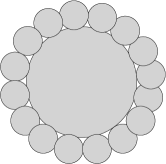
Figure 1. A flower

One can also underline that the complexity of each cell is $O(N)$. This is a direct consequence of Proposition 3 and the fact that the complexity of the union of $N$ planar discs is $O(N)$ [2, Lemma 1].

2.2. Intersection and union of confocal ellipsoids of revolution

An ellipsoid of revolution whose one focal point lies at the origin is characterized by two other parameters: its second focal point $y$ and its eccentricity $e$ in $(0,1)$. We denote the convex hull of such an ellipsoid of revolution $E(y,e)$. The surface $\partial E(y,e)$ of this set is parameterized in spherical coordinates by the function

$$\sigma_{y,e}(m):=\frac{d}{1-e\langle m|\frac{y}{\|y\|}\rangle}\quad\mbox{where }d=\frac{\|y\|(1-e^{2})}{2e}.$$

Note that the value $d$ is fully determined by $e$ and $y$ and is introduced only to simplify the computations.

Let $Y=(y_{i})_{1\leqslant i\leqslant N}$ be a family of distinct points in $\mathbb{R}^{d}$ and $e=(e_{i})_{1\leqslant i\leqslant N}$ be a family of real numbers in the interval $(0,1)$. The boundary of the intersection of solid ellipsoids $\bigcap_{1\leqslant i\leqslant N}E(y_{i},e_{i})$ is parameterized in spherical coordinates by the lower envelope of the functions $(\sigma_{y_{i},e_{i}})_{1\leqslant i\leqslant N}$. The ellipsoid intersection diagram of this family of ellipsoids is the decomposition of the unit sphere into cells associated to the lower envelope of the functions $(\sigma_{y_{i},e_{i}})_{1\leqslant i\leqslant N}$:

(2.3) $$\operatorname{EI}_{Y}^{e}(y_{i}):=\{u\in\mathcal{S}^{d-1};~{}\forall j\in\{1,\ldots,N\},\sigma_{y_{i},e_{i}}(u)\leqslant\sigma_{y_{j},e_{j}}(u)\}.$$

Similarly, the cells of the ellipsoid union diagram are associated to the upper envelope of the functions $(\sigma_{y_{i},e_{i}})_{1\leqslant i\leqslant N}$ as follows:

(2.4) $$\operatorname{EU}_{Y}^{e}(y_{i}):=\{u\in\mathcal{S}^{d-1};~{}\forall j\in\{1,\ldots,N\},\sigma_{y_{i},e_{i}}(u)\geqslant\sigma_{y_{j},e_{j}}(u)\}.$$

As in the case of paraboloids, the computation of each diagram amounts to compute the intersection of a power diagram with the unit sphere.

Proposition 7.

Let $(E(y_{i},e_{i}))_{1\leqslant i\leqslant N}$ be a family of solid confocal ellipsoids. Then,

• The cells of the ellipsoid intersection diagram are given by $\operatorname{EI}_{Y}^{e}(y_{i})=\mathcal{S}^{d-1}\cap\mathrm{Pow}_{P}^{\omega}(p_{i}),$ where $p_{i}=-\frac{e_{i}}{2d_{i}}\frac{y_{i}}{\|y_{i}\|}$ and $\omega_{i}=-\frac{1}{d_{i}}-\frac{e_{i}^{2}}{4d_{i}^{2}}.$

• The cells of the ellipsoid union diagram are given by : $\operatorname{EU}_{Y}^{e}(y_{i})=\mathcal{S}^{d-1}\cap\mathrm{Pow}_{P}^{\omega}(p_{i}),$ where $p_{i}=\frac{e_{i}}{2d_{i}}\frac{y_{i}}{\|y_{i}\|}$ and $\omega_{i}=\frac{1}{d_{i}}-\frac{e_{i}^{2}}{4d_{i}^{2}}.$

The theorem below shows that in dimension three the complexity of these diagrams can be quadratic in the number of ellipsoids. This is in sharp contrast with the case of the paraboloid intersection diagram, where the complexity is linear in the number of paraboloids.

Theorem 8.

In $\mathbb{R}^{3}$, there exists a configuration of confocal ellipsoids of revolution such that the number of vertices and edges in the ellipsoid intersection diagram (resp. the ellipsoids union diagram) is $\Omega(N^{2})$.

The proof of this theorem strongly relies on the following lemma, that transfers the problem to a complexity problem of power diagrams intersected by the unit sphere.

Lemma 9.

Let $(p_{i},\omega_{i})_{1\leqslant i\leqslant N}$ be a family of weighted points such that no point $p_{i}$ lie at the origin. Then, there exists:

• a family of ellipsoids $(E(y_{i},e_{i}))_{1\leqslant i\leqslant N}$, such that for all $i$, $\operatorname{EI}_{Y}^{e}(y_{i})=\mathcal{S}^{d-1}\cap\mathrm{Pow}_{P}^{\omega}(p_{i}).$

• a family of ellipsoids $(E(y_{i},e_{i}))_{1\leqslant i\leqslant N}$, such that for all $i$, $\operatorname{EU}_{Y}^{e}(y_{i})=\mathcal{S}^{d-1}\cap\mathrm{Pow}_{P}^{\omega}(p_{i}).$

Proof.

We prove only the first assertion, the second one being similar. Let $i\in\{1,\ldots,N\}$. By inverting the equations $p_{i}=-\frac{e_{i}}{2d_{i}}\frac{y_{i}}{\|y_{i}\|}$ and $\omega_{i}=\frac{1}{d_{i}}+\frac{e_{i}^{2}}{4d_{i}^{2}}$, we get

$$y_{i}=\frac{-4}{(\omega_{i}+\left\|p_{i}\right\|^{2})^{2}-4\left\|p_{i}\right\|^{2}}\ p_{i}\quad\mbox{and}\quad e_{i}=\frac{-2\left\|p_{i}\right\|}{\omega_{i}+\left\|p_{i}\right\|^{2}}.$$

The condition $e_{i}\in(0,1)$ is equivalent to $\omega_{i}<-\left\|p_{i}\right\|^{2}\mbox{ and }\omega_{i}<-\left\|p_{i}\right\|^{2}-\left\|p_{i}\right\|$. These inequalities can always be satisfied by substracting a large constant to all the weights $\omega_{i}$, an operation that does not change the power cells. ∎

We recall that the Voronoi diagram of a point cloud $(p_{i})_{1\leqslant i\leqslant N}$ of $\mathbb{R}^{3}$ is the decomposition of the space in $N$ convex cells defined by

$$\mathrm{Vor}_{P}(p_{i}):=\{x\in\mathbb{R}^{3},\ \left\|x-p_{i}\right\|\leqslant\left\|x-p_{j}\right\|\}.$$

The next proof is illustrated by Figure 2.

Proof of Theorem 8.

Thanks to Lemma 9, it is sufficient to build an example of Voronoi diagram whose intersection with $\mathcal{S}^{2}$ has a quadratic number of edges and vertices. We can consider without restriction that $N=2k$ is even. Let $\varepsilon>0$ be a small number. We let $p_{1},\ldots,p_{k}$ be $k$ points uniformly distributed on the circle centered at the origin in the plane $\{z=0\}$, and with radius $2-\varepsilon$. We also consider $k$ evenly distributed points $q_{1},\ldots,q_{k}$ on $(A,B)\setminus\{O\}$, where $A=(0,0,-\varepsilon/4)$, $B=(0,0,\varepsilon/4)$ and $O=(0,0,0)$. Our goal is now to show that for any $i$ and $j$ in between $1$ and $k$, the intersection $\operatorname{Vor}_{P}(p_{i})\cap\operatorname{Vor}_{P}(q_{j})\cap\mathcal{S}^{2}$ is non-empty, where $P=\{p_{i}\}\cup\{q_{j}\}$. We denote by $m_{i,j}$ the unique point which is equidistant from $p_{i}$ and $q_{j}$, and which lies in the horizontal plane containing $q_{j}$ and in the (vertical) plane passing through $p_{i}$, $q_{j}$ and the origin. A simple computation shows that the distance $\delta_{i,j}$ between $m_{i,j}$ and $q_{j}$ satisfies $\delta_{i,j}\leqslant 1-\varepsilon/2+\varepsilon^{2}/(64-32\varepsilon)$. Taking $\varepsilon$ small enough, this implies that the point $m_{i,j}$ belongs to the unit ball. The line passing through $m_{i,j}$ and orthogonal to the plane passing through $p_{i}$, $q_{j}$ and the origin cuts the unit sphere at two points $r^{\pm}_{i,j}$. These two points belong to the same horizontal plane as $q_{j}$, and they both belong to $\operatorname{Vor}_{P}(q_{j})$. Moreover, the distance between $m_{i,j}$ and each of these two points is less than $(1-\delta_{i,j}^{2})^{1/2}$. We can take $\varepsilon$ small enough so that this distance is less than $\sin(\pi/k)$. This implies that the points $r_{i,j}^{\pm}$ also belong to the Voronoi cell $\mathrm{Vor}(p_{i})$ and therefore to the intersection $\operatorname{Vor}_{P}(p_{i})\cap\operatorname{Vor}_{P}(q_{j})\cap\mathcal{S}^{2}$. Thus, the intersection between the Voronoi diagram and the sphere has at least $k^{2}=\frac{1}{4}N^{2}$ spherical edges. ∎

Figure 2. An $\Omega(N^{2})$ construction. From a total of $N$ sites, half of them in a segment inside the sphere, and half of them on a circle outside the sphere, we obtain a total of $\Omega(N^{2})$ edges embedded on the sphere.

3. Computing the intersection of a power diagram with a sphere

In this section, we describe a robust and efficient algorithm to compute the intersection between the power diagram of weighted points $(P,\omega)$ and the unit sphere. We call this intersection diagram. Given the set of weighted points $(p_{i},\omega_{i})$, we define the $i$th intersection cell as $\operatorname{ID}_{P}^{\omega}(p_{i})=\mathcal{S}^{2}\cap\operatorname{Pow}_{P}^{\omega}(p_{i})$. This algorithm is implemented using the Computational Geometry Algorithms Library (CGAL) [1], and bears some similarity to [5, 10]. We concentrate our efforts in obtaining the exact combinatorial structure of the diagram on the sphere for weighted points whose coordinates and weight are rational. Exact constructions can be obtained, but are not our focus, since in our applications, the results of this section are used as input of a numerical optimization procedure; see Section 4.

Note that the intersection diagram has complex combinatorics. If one assumes that the weighted points are given by a paraboloid intersection diagram, Proposition 3 shows that the intersection cells are connected. But even in this case, the intersection between two intersection cells $\operatorname{ID}_{P}^{\omega}(p_{i})$ and $\operatorname{ID}_{P}^{\omega}(p_{j})$ can have multiple connected components. Consequently, one cannot hope to be able to reconstruct these cells from the adjacency graph (i.e., the graph that contains the points in $P$ as vertices, and where two vertices are connected by an arc if the two cells intersect in a non-trivial circular arc), even in this simple case. In general, the cells of the intersection diagram can be disconnected and they can have holes, as shown in Figure 3. In the next paragraph, we propose an algorithm to compute a boundary representation of these cells. Recall the following definitions concerning power diagrams:

Definition 3.1.

When two power cells $\operatorname{Pow}_{P}^{\omega}(p_{i})\cap\operatorname{Pow}_{P}^{\omega}(p_{j})$ intersect in a $2$-dimensional set, that is a (possibly unbounded) polygon in $\mathbb{R}^{3}$, they determine a facet of the power diagram. Similarly, a ridge is a $1$-dimensional intersection $\operatorname{Pow}_{P}^{\omega}(p_{i})\cap\operatorname{Pow}_{P}^{\omega}(p_{j})\cap\operatorname{Pow}_{P}^{\omega}(p_{k})$ between three power cells. A ridge can be either a ray or a segment. The boundary of each facet can be written as a finite union of ridges.

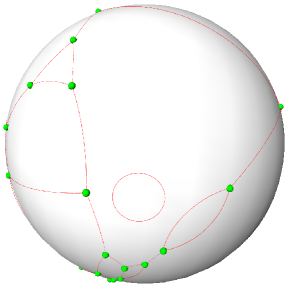
(a) general

(b) cube

Figure 3. Examples of diagram on the sphere. Left: an intersection diagram containing faces with no vertices, faces with holes and faces with two vertices or more. Right: a diagram corresponding to the intersection of a cube and a sphere; there are seven faces, six faces with no vertices, and a face with no vertices and six holes.

In the remainder of this section, we explain how to compute a single intersection cell $\operatorname{ID}_{P}^{\omega}(p_{i})$, for a given $p_{i}$, without any assumption on the points and weights. This intersection cell can be quite intricate (multiple connected components, holes), and will therefore be represented by its oriented boundary. More precisely, the boundary $\operatorname{ID}_{P}^{\omega}(p_{i})$ is a finite union of closed curves called cycles. These cycles are oriented so that for someone walking on the sphere following a cycle, the intersection cell $\operatorname{ID}_{P}^{\omega}(p_{i})$ lies to the right. The cell is uniquely determined by its oriented boundary. The following theorem is the main result of this section.

Theorem 10.

There is an $O(N\log N+C)$ algorithm for obtaining the intersection diagram of a set $P$ of $N$ weighted points in $\mathbb{R}^{3}$, where $C$ is the complexity of the power diagram of $P$.

From Theorem 8, the size of the output in the worst case for the intersection (or union) of confocal ellipsoids is $\Omega(N^{2})$. This implies that the algorithm described below is optimal for computing an ellipsoid intersection (or union) diagram. The optimality of the algorithm for the paraboloid intersection diagram is an open problem, which can be phrased as follows:

Open Question 11.

Is the complexity of the power diagram given by Proposition 1 bounded by $O(N)$ ?

Remark.

Even if the question above has a negative answer, at least for the particular case of the intersection diagram of confocal paraboloids, there exists an easy randomized incremental algorithm attaining the lower bound in Proposition 4. If the input is $N$ confocal paraboloids, from Theorem 2, we know that the complexity of the paraboloid intersection diagram is $O(N)$. Moreover the resulting cells are connected. Adopting the randomized incremental construction paradigm (see [20, 16] for a comprehensive study), this means that the expected complexity of the cell of the $i$th inserted paraboloid is $O(N)/i$. Besides, thanks to the connectedness of the cells, we can detect the conflicts with a breadth-first search in linear time as well, without any additional structure. Therefore, the total expected cost is $\sum_{i=1}^{n}O(N)/i$, which is in $O(N\log{N})$. Notice that this analysis relies on the fact that the cells are connected, which is not necessarily true in the case of union of paraboloids and in the ellipsoids cases. In our application, we always use the generic and robust algorithm based on the intersections of power cells, using CGAL.

3.1. Predicates

Geometric algorithms often rely on predicates, i.e., estimation of finite-valued geometric quantities such as the orientation of a quadruple of points in $3$D, or the number of intersections between a straight line and a surface. These predicates need to be evaluated exactly: if this is not the case, some geometric algorithm may even not terminate [12]. We adopt the dynamic filtering technique for the computation of our predicates in CGAL. This means that for every arithmetic operation, we also compute an error bound for the result. This can be automatized using interval arithmetic [6]. If the error bound is too large to determine the result of the predicate, the arithmetic operation is performed again with exact rational arithmetic, allowing us to return an exact answer for the predicate. Our algorithm requires the following three predicates:

• has_on(Point p) returns $+1$, $0$, or $-1$, if the point is outside, on, or inside the unit sphere respectively.

• number_of_intersections(Ridge r) returns the number of intersections between $r$ and the unit sphere ($0,1$ or $2$), where $r$ can be a segment or a ray. By convention, segment or ray touching the sphere tangentially has two intersection points, with same coordinates. Remark that the result of the first predicate can be obtained directly from the intermediate computations of this predicate. As we use them intertwined, this shortcut is adopted in our implementation.

• plane_crossing_sphere(Facet f) returns the number of intersections between the supporting plane of $f$ and the sphere ($0,1$ or $+\infty$). One may notice that this predicate is just the dual of the first one.

Even though the algorithm below is presented as working directly on the cells of the power diagram, our actual implementation uses CGAL, and we work with the regular triangulation of the set of points (that is, the dual of the power diagram). This triangulation is a simplicial complex with $0$-, $1$-, $2$- and $3$-simplices. In CGAL, only the $0$- and $3$-simplices are actually stored in memory, but it remains possible to traverse the whole structure in linear time in the number of simplices. In order to handle the boundary simplices, CGAL takes the usual approach of adding a point at infinity to the initial set of points. In practice, this means the following. A ridge of the power digram can be either a segment or a ray, and is dual of a $2$-simplex in the triangulation. In CGAL, such a ridge corresponds to two adjacent tetrahedra, one of whom may contain the point at infinity. The predicates above need to be adapted in order to handle $k$-simplices that are incident to the point at infinity. The general predicates have been implemented, but the details are omitted here.

3.2. Computation of the oriented boundary

The output of our algorithm is the oriented boundary of the intersection cell $\operatorname{ID}_{P}^{\omega}(p_{i})$. Note that this is a purely combinatorial object, and no geometric construction are performed during its computation. It is described as a sequence of vertices on the sphere, oriented arcs, and oriented cycles.

(a) inside

(b) intersecting

(c) enclosing

Figure 4. Obtaining the arcs of $\operatorname{ID}_{P}^{\omega}(p_{i})$. Three distinct cases: (a) inside the circle, (b) intersecting the circle, and (c) enclosing the circle. There is still a case not depict above, $f$ can be outside the circle as well. The arcs with zero length, such as the one in (b) can be removed from the diagram depending on its use.

$\bullet$ A vertex on the sphere is the result of an intersection between a ridge of the power diagram and the unit sphere. A vertex on the sphere is not constructed explicitly, but stored as an ordered pair of extremities of the corresponding ridge. Since a ridge $[x_{1},x_{2}]$ can intersect the sphere twice, the order determines which intersection point to consider, i.e., the pair $(x_{1},x_{2})$ describes the intersection point that is closest to $x_{1}$. This convention allows us to handle infinite ridges, and to uniquely identify vertices on the sphere. In degenerate cases, vertices may correspond to different ordered pairs, but having the same coordinates.

$\bullet$ An oriented arc corresponds to the (oriented) intersection between $\operatorname{Pow}_{P}^{\omega}(p_{i})$, another cell $\operatorname{Pow}_{P}^{\omega}(p_{j})$ and the unit sphere. Two situations arise. Either the arc is a complete circle, in which case it is also a cycle. Or the two extreme points are vertices as defined above, that is, they are the intersection between ridges and the unit sphere. An arc is oriented so that, when walking on the sphere from the first point to the second, the cell lies on the right.

$\bullet$ An oriented cycle is a connected component of the oriented boundary of $\operatorname{ID}_{P}^{\omega}(p_{i})$. A cycle can have two or more vertices on the sphere, in this case, they are represented by a cyclic sequence of arcs. However, a cycle can also have no vertices, and in such a case, it is represented by a single full arc. The orientation of a cycle is given by the orientation of its arcs.

Notice that the boundary of a power cell is composed of several convex facets, that can possibly be unbounded. The intersection of such facets with the unit sphere gives the arcs of the intersection diagram. Our algorithm constructs the oriented boundary of the intersection cell $\operatorname{ID}_{P}^{\omega}(p_{i})$ by iterating over each facet of the power cell $\operatorname{Pow}_{P}^{\omega}(p_{i})$ and obtaining implicitly both the set of vertices on the sphere $V$ and the set of oriented arcs $E$. The oriented graph $G=(V,E)$ is called the boundary graph. Once $G$ is constructed, the oriented cycles in the boundary $\partial\operatorname{ID}_{p}^{\omega}(p_{i})$ coincide with the (oriented) connected components of $G$, and can be obtained by a simple traversal. In the next paragraph, we explain the construction of $G=(V,E)$.

3.3. Computation of the boundary graph

We start by discarding the facets that do not contribute to the intersection diagram. We iterate over all facets $f$ of $\operatorname{Pow}_{P}^{\omega}(p_{i})$, and keep $f$ only if the predicate plane_crossing_sphere$(f)$ returns $\infty$. (The case where it returns $1$ corresponds to a trivial intersection between the facet and the sphere and can be safely ignored.) Assuming that $f$ is not discarded, the intersection of its supporting plane with the unit sphere is a circle in $3$D. If all vertices of $f$ are on or inside the sphere (i.e., has_on$\leqslant 0$), then $f$ is inside or only touching the circle, and is discarded. See Figure LABEL:sub@fig:obtaining_arcs:inside.

Given a facet $f=\operatorname{Pow}_{P}^{\omega}(p_{i})\cap\operatorname{Pow}_{P}^{\omega}(p_{j})$ that was not discarded previously, we build a sequence of vertices on the sphere by traversing $f$ in a clockwise sequence of ridges, oriented with respect to the vector $p_{j}-p_{i}$ . We distinguish two different kinds of vertices on the sphere, the source vertices and the target vertices, as shown on Figure LABEL:sub@fig:obtaining_arcs:intersecting. Given an oriented ridge $r=[x_{1},x_{2}]$, we compute the value of number_of_intersections(r). If the ridge has zero intersections with the sphere, we skip it. If there is only one intersection between $r$ and the unit sphere, the corresponding vertex is a source if $x_{1}$ is inside the sphere (i.e., has_on(x_1) $\leqslant 0$) and it is a target vertex in the other case. Finally, if the ridge intersects the sphere twice, the oriented pair $(x_{1},x_{2})$ describes the target vertex, and the pair $(x_{2},x_{1})$ is the source vertex. The arcs of the boundary graph $G$ corresponding to this facet are obtained by matching each source vertex with a target vertex using the same cyclic sequence. They are represented by an ordered pair of vertex indices.

Finally, we need to consider the case where none of the ridges of $f$ intersect the sphere. There are two possibilities: either the facet $f$ encloses the circle $\pi\cap\mathcal{S}^{2}$, where $\pi$ is the affine plane spanned by $f$, or the circle is completely outside from $f$. In the former case, we obtain an arc without vertex in the boundary of $\operatorname{ID}_{P}^{\omega}(p_{i})$, as shown in Figure LABEL:sub@fig:obtaining_arcs:enclosing. Its orientation is clockwise with respect to the vector $p_{j}-p_{i}$. To detect whether this happens, we simply need to determine whether the center of the circle lies inside or outside the convex polygon $f$. This is a classical routine that can be performed using signed volumes. For this test, we only need to use rational numbers because the center of the circle is the projection of the origin on a plane described with rational coordinates.

Proof of Theorem 10.

First we build the regular triangulation of the set of $N$ weighted points in $O(N\log N+C)$ time. Running the algorithm described in this section for every $p_{i}$ makes us visiting each $1$-simplex, $2$-simplex, and $3$-simplex of the primal no more than two, three, and four times respectively; and for each visit, it takes $O(1)$ time, since we compute constant-degree predicates. Then we visit each generated cycle at most twice. Therefore, the complexity of our algorithm is in $O(N\log N+C+D)$, where $D$ is the complexity of the diagram on the sphere. The fact that $D=O(C)$ completes the proof. ∎

4. Application to Minkowski-type problems involving paraboloids

This section deals with the far-field reflector problem [9], which is a Minkowski-type problem involving intersection of confocal paraboloids of revolution. Consider a point source light located at the origin $O$ of $\mathbb{R}^{d}$ that emits lights in all directions. The intensity of the light emitted in the direction $x\in\mathcal{S}^{d-1}$ is denoted by $\rho(x)$. Now, consider a hypersurface $R$ of $\mathbb{R}^{d}$. By Snell’s law, every ray $x$ emitted by the source light that intersects $R$ at a point whose normal vector is $n$ is reflected in the direction $y=x-2\langle x|n\rangle n$. This means that after reflection on $R$, the distribution of light at the origin given by $\rho$ is transformed into a distribution $\nu_{R}$ on the set of directions at infinity, a set that can also be described by the unit sphere. The far-field reflector problem consists in the following inverse problem: given a density $\rho$ on the source sphere $\mathcal{S}^{2}$ and a distribution $\mu$ on the sphere at infinity, the problem is to find an hypersurface $R$ such that $\mu_{R}$ coincides with $\mu$. For computational purposes, we assume that the target measure $\nu$ is supported on a finite set of directions $Y:=(y_{i})_{1\leqslant i\leqslant N}$, and it is thus natural to consider a reflector made of pieces of paraboloids with directions $Y$. This problem is numerically solved using an optimal transport formulation due to [21, 11].

(a) Initial $(\lambda_{i})_{1\leqslant i\leqslant N}$

(b) Final $(\lambda_{i})_{1\leqslant i\leqslant N}$

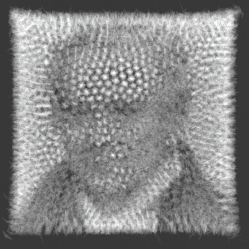
(c) Rendering

(d) Final $(\lambda_{i})_{1\leqslant i\leqslant N}$

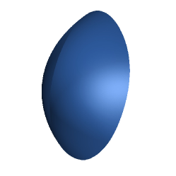
(e) Reflector

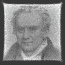
(f) Rendering

Figure 5. Numerical computation. Calculations were done with $N=1000$ paraboloids for the first row and $N=15000$ paraboloids for the second row. (a) Paraboloid intersection diagram for an initial $(\lambda_{i})_{1\leqslant i\leqslant N}$. (b,d) Final intersection diagram after optimization. (e) Reflector surface defined by the intersection of paraboloids. (c,f) Simulation of the illumination at infinity from a punctual light source lighting uniformly $\mathcal{S}_{-}^{2}$, using LuxRender, a physically accurate raytracer engine.

4.1. Far-field reflector problem.

We consider a finite family $Y=(y_{1},\ldots,y_{N})$ of unit vectors that describe directions at infinity, non-negative numbers $(\alpha_{i})_{1\leqslant i\leqslant N}$ such that $\sum_{1\leqslant i\leqslant N}\alpha_{i}=1$ and a probability density $\rho$ on the unit sphere. The far-field reflector problem consists in finding a vector of non-negative focal distances $(\lambda_{i})_{1\leqslant i\leqslant N}$, such that

(FF) $$\forall i\in\{1,\ldots,N\},~{}~{}\rho(\operatorname{PI}_{Y}^{\lambda}(y_{i}))=\alpha_{i},$$

where for a subset $X$ of the sphere, $\rho(X):=\int_{X}\rho(u)\mathrm{d}u$ is the weighted area of $X$. The far-field reflector problem can be transformed into the maximization of a concave functional, combining ideas from [21, 11, 3].

Theorem 12.

A vector of focal distances $(\lambda_{i})_{1\leqslant i\leqslant N}$ solves the far-field reflector problem (FF) if and only if the vector $(\gamma_{i})_{1\leqslant i\leqslant N}$ defined by $\gamma_{i}=\log(\lambda_{i})$ is a global maximizer of the following $\mathcal{C}^{1}$ concave function:

(4.5) $$\Phi(\gamma):=\left[\sum_{i=1}^{N}\int_{\operatorname{PI}_{Y}^{\exp\gamma}(y_{i})}(c(u,y_{i})+\gamma_{i})\rho(u)\mathrm{d}u\right]-\sum_{i=1}^{N}\gamma_{i}\alpha_{i}$$

where $c(u,v):=-\log(1-\langle u|v\rangle)$ and with the convention $\log(0)=-\infty$. Moreover, the gradient of the function $\Phi$ is given by

(4.6) $$\nabla\Phi(\gamma):=(\rho(\operatorname{PI}_{Y}^{\exp(\gamma)}(y_{i}))-\alpha_{i})_{1\leqslant i\leqslant N}.$$

There is a similar formulation for a reflector defined by the union of solid confocal paraboloids [11]. However, there is no known variational formulation for the reflector problem involving intersection of ellipsoids. A numerical approach has been proposed in [18].

We now turn to the proof of Theorem 12. This proof combines the results of Section 5 of [3] with the optimal transport formulation of the far-field reflector problem [21, 11]. Let us first recall some properties of supdifferential of concave functions. Given a function $\Phi$ and $\lambda$ in $\mathbb{R}^{N}$, the supdifferential of $\Phi$ at $\lambda$, denoted $\partial^{+}\Phi(\lambda)$ is the set of vectors $v$ such that

$$\forall\kappa\in\mathbb{R}^{N},~{}\Phi(\kappa)\leqslant\Phi(\lambda)+\langle\kappa-\lambda|v\rangle.$$

A function $\Phi$ is concave if and only if for every $\lambda$, the supdifferential $\partial^{+}\Phi(\lambda)$ is nonempty. If this is the case, $\Phi$ is differentiable almost everywhere, and at points of differentiability the supdifferential $\partial^{+}\Phi(\lambda)$ coincides with the singleton $\{\nabla\Phi(\lambda)\}$. Finally, $\lambda$ is a global maximum of $\Phi$ if and only if $\partial^{+}\Phi(\lambda)$ contains the zero vector.

Proof of Theorem 12.

We consider a vector $\gamma$ in $\mathbb{R}^{N}$. First remark that $c(u,y_{i})+\gamma_{i}=\log(\exp(\gamma_{i})/(1-\langle u|y_{i}\rangle)$. Therefore,

$$u\in\operatorname{PI}_{Y}^{\exp(\gamma)}(y_{i}) \Longleftrightarrow\forall j\in\{1,\ldots,N\},\frac{\exp(\gamma_{i})}{1-\langle u|y_{i}\rangle}\leqslant\frac{\exp(\gamma_{j})}{1-\langle u|y_{j}\rangle}$$

$$\Longleftrightarrow\forall j\in\{1,\ldots,N\},c(u,y_{i})+\gamma_{i}\leqslant c(u,y_{j})+\gamma_{j}$$

Therefore, the function $\Phi$ can be reformulated as follows:

$$\Phi(\gamma)=\int_{\mathcal{S}^{d-1}}\left(\min_{1\leqslant i\leqslant N}c(u,y_{i})+\gamma_{i}\right)\rho(u)\mathrm{d}u-\sum_{i=1}^{N}\gamma_{i}\alpha_{i}.$$

We now define $T_{\gamma}$ as the function that maps a point $u$ on the unit sphere to the point $y_{i}$ such that $u$ belongs to $\operatorname{PI}_{Y}^{\exp(\gamma)}(y_{i})$. Then,

(4.7) $$\Phi(\gamma)=\int_{\mathcal{S}^{d-1}}(c(u,T_{\gamma}(u))+\gamma_{T_{\gamma}(u)})\rho(u)\mathrm{d}u-\sum_{i=1}^{N}\gamma_{i}\alpha_{i}.$$

Moreover, for any $\kappa$ in $\mathbb{R}^{d}$, one has $\min_{1\leqslant i\leqslant N}c(u,y_{i})+\kappa_{i}\leqslant c(u,T_{\gamma}(u))+\kappa_{T_{\gamma}(u)}$. Integrating this inequality, and substracting (4.7), we get

$$\Phi(\kappa)-\Phi(\gamma) \leqslant\int_{\mathcal{S}^{d-1}}(\kappa_{T_{\gamma}(u)}-\gamma_{T_{\gamma}(u)})\rho(u)\mathrm{d}u-\sum_{1\leqslant i\leqslant N}(\kappa_{i}-\gamma_{i})\alpha_{i}$$

$$\leqslant\sum_{1\leqslant i\leqslant N}\left(\int_{\operatorname{PI}_{Y}^{\exp\gamma}(y_{i})}\rho(u)\mathrm{d}u-\alpha_{i}\right)(\kappa_{i}-\gamma_{i})=\langle D\Phi(\gamma)|\kappa-\gamma\rangle$$

(4.8) $$\hbox{where }D\Phi(\gamma) :=(\rho(\operatorname{PI}_{Y}^{\exp(\gamma)}(y_{i}))-\alpha_{i})_{1\leqslant i\leqslant N}.$$

The above inequality shows that $D\Phi(\gamma)$ lies in $\partial^{+}\Phi(\gamma)$, i.e., this set is never empty and the function $\Phi$ is concave. Since the vector $D\Phi(\gamma)$ depends continuously on $\gamma$, we deduce that the function $\Phi$ is $\mathcal{C}^{1}$ smooth, and that $\nabla\Phi(\gamma)=D\Phi(\gamma)$ everywhere. By Equation (4.8), a vector $\lambda:=\exp(\gamma)$ solves the far-field reflector problem (FF) if and only if $D\Phi(\gamma)=0$, i.e., if and only if $\gamma$ is a global maximizer of $\Phi$. ∎

4.2. Implementation details.

The implementation of the maximization of the functional $\Phi$ follows closely [15]. We rely on a quasi-Newton method, which only requires being able to evaluate the value of $\Phi$ and the value of its gradient at any point $\gamma$, as given by Equations (4.5)–(4.6). The computations of these values are performed in two steps. First, we compute the boundary of the paraboloid intersection cells $\operatorname{PI}_{Y}^{\exp(\gamma)}(y_{i})$, using the algorithm described in Section 3. These cells are then tessellated, and the integrals in Equations (4.5)–(4.6) are evaluated numerically using a simple Gaussian quadrature. In the experiments illustrated in Figure 5, we constructed the measure $\sum_{i}\alpha_{i}\delta_{y_{i}}$ so as to approximate a picture of Gaspard Monge (projected on a part of the half-sphere $\mathcal{S}^{2}_{+}:=\mathcal{S}^{2}\cap\{z\geqslant 0\}$). The density $\rho$ is constant in the half-sphere $\mathcal{S}^{2}_{-}$ and vanishes in the other half. To the best of our knowledge, the only other numerical implementation of this formulation of the far-field reflector problem has been proposed in [8]. The authors develop an algorithm, called Supporting paraboloids which bears resemblance to Bertsekas’ auction algorithm for the assignment problem [4]. They use it to solve the far-field reflector problem with 19 paraboloids. Using the quasi-Newton approach presented above, and the algorithm developed in Section 3, we are able to solve this problem for 15,000 paraboloids in less than 10 minutes on a desktop computer. Note that the algorithm of Section 3 would probably also allow a faster and robust implementation of the Supporting paraboloids algorithm [8].

5. Conclusion

In addition to the open problems mentioned earlier, let us mention a perspective. In a recent article [13], the algorithm of supporting paraboloids was extended to optimal transport problems involving a cost function $c$ that satisfies the so-called Ma-Trudinger-Wang regularity condition. For this algorithm to be practical, one needs to compute the generalized Voronoi cells efficiently, defined for any function $\psi:Y\to\mathbb{R}$ by

$$\operatorname{Vor}_{c}^{\psi}(y)=\{x\in X;~{}\forall z\in Y,~{}c(x,y)+\psi(y)\leqslant c(x,z)+\psi(z)\}.$$

For general costs, and even in $2$D, one cannot hope to do this in time below $\Omega(N^{2})$. However, the MTW regularity condition ensures an analog of Proposition 3 and in particular, it implies that these generalized Voronoi cells are connected. One might wonder whether a randomized iterative construction could be used in this setting to yield a construction in expected time $O(N\log N)$ in $2$D. This would open the way to practical algorithms for the resolution of optimal transport problems that are intractable to PDE-based methods.

5.1. Acknowledgements.

The authors would like to thank Dominique Attali, Olivier Devillers and Francis Lazarus for interesting discussions. Olivier Devillers suggested the approach used in the proof of the lower complexity bound for intersection of ellipsoids. The first author is supported by grant FACEPE/INRIA,APQ-0055-1.03/12. The second and third author would like to acknowledge the support of the French Agence Nationale de la Recherche (ANR) under reference ANR-11-BS01-014-01 (TOMMI) and ANR-13-BS01-0008-03 (TOPDATA) respectively.

References

- [1] Cgal, Computational Geometry Algorithms Library, http://www.cgal.org.
- [2] F. Aurenhammer, Power diagrams: properties, algorithms and applications, SIAM Journal of Computing 16 (1987), 78–96.
- [3] F. Aurenhammer, F. Hoffmann, and B. Aronov, Minkowski-type theorems and least-squares clustering, Algorithmica 20 (1998), no. 1, 61–76.
- [4] D. P. Bertsekas and J. Eckstein, Dual coordinate step methods for linear network flow problems, Mathematical Programming 42 (1988), no. 1, 203–243.
- [5] J.-D. Boissonnat and M. I. Karavelas, On the combinatorial complexity of euclidean Voronoi cells and convex hulls of d-dimensional spheres, Proceedings of the fourteenth annual ACM-SIAM symposium on Discrete algorithms (Philadelphia, PA, USA), SODA ’03, Society for Industrial and Applied Mathematics, 2003, pp. 305–312.
- [6] H. Brónnimann, C. Burnikel, and S. Pion, Interval arithmetic yields efficient dynamic filters for computational geometry, Discrete Applied Mathematics 109 (2001), 25–47.
- [7] L. A. Caffarelli, C. E. Gutiérrez, and Q. Huang, On the regularity of reflector antennas, Annals of Mathematics-Second Series 167 (2008), no. 1, 299.
- [8] L. A. Caffarelli, S. Kochengin, and V. I. Oliker, On the numerical solution of the problem of reflector design with given far-field scattering data, Contemporary Mathematics 226 (1999), 13–32.
- [9] L. A. Caffarelli and V. I. Oliker, Weak solutions of one inverse problem in geometric optics, Journal of Mathematical Sciences 154 (2008), no. 1, 39–49.
- [10] C. Delage, Cgal-based first prototype implementation of moebius diagram in 2D, 2008.
- [11] T. Glimm and V. Oliker, Optical design of single reflector systems and the monge–kantorovich mass transfer problem, Journal of Mathematical Sciences 117 (2003), no. 3, 4096–4108.
- [12] L. Kettner, K. Mehlhorn, S. Schirra, and C. K. Yap, Classroom examples of robustness problems in geometric computations, Computational Geometry: Theory and Applications 40 (2008), 61–79.
- [13] Jun Kitagawa, An iterative scheme for solving the optimal transportation problem, arXiv preprint arXiv:1208.5172 (2012).
- [14] S. A. Kochengin and V. I. Oliker, Determination of reflector surfaces from near-field scattering data, Inverse Problems 13 (1997), no. 2, 363.
- [15] Q. Mérigot, A multiscale approach to optimal transport, Computer Graphics Forum, vol. 30, Wiley Online Library, 2011, pp. 1583–1592.
- [16] K. Mulmuley (ed.), Computational geometry - an introduction through randomized algorithms., Prentice Hall, 1994.
- [17] V. I. Oliker, Mathematical aspects of design of beam shaping surfaces in geometrical optics, Trends in Nonlinear Analysis (2003), 193–224.
- [18] by same author, A rigorous method for synthesis of offset shaped reflector antennas, Computing Letters 2 (2006), no. 1-2, 1–2.
- [19] by same author, A characterization of revolution quadrics by a system of partial differential equations, Proceedings of the American Mathematical Society 138 (2010), no. 11, 4075–4080.
- [20] J.-R. Sack and J. Urrutia (eds.), Handbook of computational geometry, North-Holland Publishing Co., 2000.
- [21] X.J. Wang, On the design of a reflector antenna ii, Calculus of Variations and Partial Differential Equations 20 (2004), no. 3, 329–341.