Multi-Objective Resource Allocation for Secure Communication in Cognitive Radio Networks with Wireless Information and Power Transfer

Abstract

In this paper, we study resource allocation for multiuser multiple-input single-output (MISO) secondary communication systems with multiple system design objectives. We consider cognitive radio (CR) networks where the secondary receivers are able to harvest energy from the radio frequency when they are idle. The secondary system provides simultaneous wireless power and secure information transfer to the secondary receivers. We propose a multi-objective optimization framework for the design of a Pareto optimal resource allocation algorithm based on the weighted Tchebycheff approach. In particular, the algorithm design incorporates three important system design objectives: total transmit power minimization, energy harvesting efficiency maximization, and interference power leakage-to-transmit power ratio minimization. The proposed framework takes into account a quality of service (QoS) requirement regarding communication secrecy in the secondary system and the imperfection of the channel state information (CSI) of potential eavesdroppers (idle secondary receivers and primary receivers) at the secondary transmitter. The proposed framework includes total harvested power maximization and interference power leakage minimization as special cases. The adopted multi-objective optimization problem is non-convex and is recast as a convex optimization problem via semidefinite programming (SDP) relaxation. It is shown that the global optimal solution of the original problem can be constructed by exploiting both the primal and the dual optimal solutions of the SDP relaxed problem. Besides, two suboptimal resource allocation schemes for the case when the solution of the dual problem is unavailable for constructing the optimal solution are proposed. Numerical results not only demonstrate the close-to-optimal performance of the proposed suboptimal schemes, but also unveil an interesting trade-off between the considered conflicting system design objectives.

I Introduction

The explosive growth of the demand for ubiquitous, secure, and high data rate wireless communication services has led to a tremendous solicitation of limited radio resources such as bandwidth and energy. In practice, fixed spectrum allocation has been implemented for resource sharing in traditional wireless communication systems. Although interference can be avoided by assigning different wireless services to different licensed frequency bands, such a fixed spectrum allocation strategy may result in spectrum under utilization. In fact, the Federal Communications Commission (FCC) has reported that $70$ percent of the allocated spectrum in the United States is not fully utilized, cf. [2]. As a result, cognitive radio (CR) has emerged as one of the most promising solutions to improve spectrum efficiency [3]. In particular, CR enables a secondary system to access the spectrum of a primary system as long as the interference from the secondary system does not severely degrade the quality of service (QoS) of the primary system [2]–[11]. CR is not only applicable to traditional cellular networks, but also has the potential to improve the performance of wireless sensor networks [5, 6]. In [7] and [8], cooperative spectrum sensing and the sensing-throughput trade-off were studied for single antenna systems, respectively. In [9], joint beamforming and power control was studied for transmit power minimization in multiple-transmit-antenna CR downlink systems. In [10] and [11], by taking into account the imperfectness of channel state information, robust beamforming designs were proposed for CR networks with single and multiple secondary users, respectively. Furthermore, a detailed performance analysis of transmit antenna selection in multiple-antenna networks was presented in [12] for multi-relay networks and then extended to CR relay networks in [13]. However, since the transmit precoding strategies in [12] and [13] are not optimized, they do not fully exploit the available degrees of freedom in the network for maximizing the system performance.

Although the current spectrum scarcity may be partially overcome by CR technology, wireless communication devices, such as wireless sensors, are often powered by batteries with limited energy storage capacity. This constitutes another major bottleneck for providing communication services and extending the lifetime of networks. On the other hand, energy harvesting is envisioned to provide a perpetual energy source to facilitate self-sustainability of power-constrained communication devices [14]–[24]. In addition to conventional renewable energy sources such as biomass, wind, and solar, wireless power transfer has emerged as a new option for prolonging the lifetime of battery-powered wireless devices. Specifically, the transmitter can transfer energy to the receivers via electromagnetic waves in radio frequency (RF). Nowadays, energy harvesting circuits are able to harvest microwatt to milliwatt of power over the range of several meters for a transmit power of $1$ Watt and a carrier frequency of less than $1$ GHz [14]. Thus, RF energy can be a viable energy source for devices with low-power consumption, e.g. wireless sensors [16, 17]. The integration of RF energy harvesting capabilities into communication systems provides the possibility of simultaneous wireless information and power transfer (SWIPT) [16]–[24]. As a result, in addition to the traditional QoS constraints such as communication reliability, efficient energy transfer is expected to play an important role as a new QoS requirement. This new requirement introduces a paradigm shift in the design of both resource allocation algorithms and transceiver signal processing. In [19] and [20], the fundamental trade-off between the maximum achievable data rate and energy transfer was studied for a noisy single-user communication channel and a pair of noisy coupled-inductor circuits, respectively. Then, in [21], the authors extended the trade-off study to a two-user multiple-antenna transceiver system. In [22], the authors proposed separated receivers for SWIPT to facilitate low-complexity receiver design; these receivers can be built by using off-the-shelf components. In [23], different resource allocation algorithms were designed for broadband far field wireless systems with SWIPT. In [24], the authors showed that the energy efficiency of a communication system can be improved by RF energy harvesting at the receivers. Nevertheless, resource allocation algorithms maximizing the energy harvesting efficiency of SWIPT CR systems have not been reported in the literature yet. Besides, two conflicting system design objectives arise naturally for a CR network providing SWIPT service to the secondary receivers in practice. On the one hand, the secondary transmitter should transmit with high power to facilitate energy transfer to the energy harvesting receivers. On the other hand, the secondary transmitter should transmit with low power to cause minimal interference at the primary receivers. Thus, considering these conflicting system design objectives, the single objective resource allocation algorithms proposed in [19]–[24] may not be applicable in SWIPT CR networks. Furthermore, transmitting with high signal power may also cause substantial information leakage and high vulnerability to eavesdropping.

Recently, physical (PHY) layer security has attracted much attention in the research community for preventing eavesdropping [25]–[34]. In [25], the authors proposed a beamforming scheme for maximization of the energy efficiency of secure communication systems. In [26] and [27], the spatial degrees of freedom offered by multiple antennas were used to degrade the channel of the eavesdroppers deliberately via artificial noise transmission. Thereby, communication secrecy was guaranteed at the expense of allocating a large portion of the transmit power to artificial noise generation. In [28], the authors addressed the power allocation problem in CR secondary systems with PHY layer security provisioning. However, the resource allocation algorithm designs in [25]–[28] cannot be directly extended to the case of of RF energy harvesting due to the differences in the underlying system models. On the other hand, [1] and [30] studied different resource allocation algorithms for providing secure communication in systems with separated information and energy harvesting receivers. Yet, the assumption of having perfect channel state information (CSI) of the energy harvesting receivers in [1] and [30] may be too optimistic if the energy harvesting receivers do not interact with the transmitter periodically. In [29], the case where the transmitter has only imperfect CSI of the energy harvesting receivers was considered and a robust beamforming design was proposed to minimize the total transmit power of a system with simultaneous energy and secure information transfer. In [31], the authors studied resource allocation algorithm design for secure information and renewable green energy transfer to mobile receivers in distributed antenna communication systems. In [32] and [33], beamforming algorithm design and secrecy outage capacity was studied for multiple-antenna potential eavesdropper and passive eavesdroppers, respectively. However, the beamforming algorithms developed in [29]–[32] may not be applicable in CR networks. Furthermore, in [34], the secrecy outage probability of CR networks was investigated in the presence of a passive eavesdropper.

Form the above discussions, we conclude that for CR communication systems providing simultaneous wireless energy transfer and secure communication services, conflicting system design objectives such as total transmit power minimization, energy harvesting efficiency maximization, and interference power leakage-to-transmit power ratio minimization play an important role for resource allocation. However, the problem formulations in [19]–[34] focus on a single system design objective and cannot be used to study the trade-off between the aforementioned conflicting design goals. In this paper, we address the above issues and the contributions of the paper are summarized as follows:

• Different from our previous work in [29], in this paper, we propose a new non-convex multi-objective optimization problem with the aim to jointly minimize the total transmit power, maximize the energy harvesting efficiency, and minimize the interference power leakage-to-transmit power ratio for CR networks with SWIPT. The problem formulation takes into account the imperfectness of the CSI of potential eavesdroppers (idle secondary receivers) and primary receivers in secondary multiuser multiple-input single-output (MISO) systems with RF energy harvesting receivers. The solution of the optimization problem leads to a set of Pareto optimal resource allocation policies.

• The considered non-convex optimization problem is recast as a convex optimization problem via semidefinite programming (SDP) relaxation. We show that the global optimal solution of the original problem can be constructed by exploiting both the primal and the dual optimal solutions of the SDP relaxed problem.

• The obtained solution structure is also applicable to the multi-objective optimization of the total harvested power, the interference power leakage, and the total transmit power.

• Two suboptimal resource allocation schemes are proposed for the case when the solution of the dual problem of the SDP relaxed problem is unavailable for construction of the optimal solution.

Our results unveil a non-trivial trade-off between the considered system design objectives which can be summarized as follows: (1) A resource allocation policy minimizing the total transmit power also leads to a low total interference power leakage in general; (2) energy harvesting efficiency maximization and transmit power minimization are conflicting system design objectives; (3) the maximum energy harvesting efficiency is achieved at the expense of high interference power leakage and high transmit power.

II System Model

In this section, we first introduce the notation used in this paper. Then, we present the adopted CR downlink channel model for secure communication with SWIPT.

II-A Notation

We use boldface capital and lower case letters to denote matrices and vectors, respectively. For a square-matrix $\mathbf{S}$, $\operatorname{\mathrm{Tr}}(\mathbf{S})$ denotes the trace of matrix $\mathbf{S}$. $\mathbf{S}\succ\mathbf{0}$ and $\mathbf{S}\succeq\mathbf{0}$ indicate that $\mathbf{S}$ is a positive definite and a positive semidefinite matrix, respectively. $(\mathbf{S})^{H}$ and $\operatorname{\mathrm{Rank}}(\mathbf{S})$ denote the conjugate transpose and the rank of matrix $\mathbf{S}$, respectively. $\mathbf{I}_{N}$ denotes an $N\times N$ identity matrix. $\mathbb{C}^{N\times M}$ and $\mathbb{R}^{N\times M}$ denote the space of $N\times M$ matrices with complex and real entries, respectively. $\mathbb{H}^{N}$ represents the set of all $N$-by-$N$ complex Hermitian matrices. $\lvert\cdot\rvert$ and $\lVert\cdot\rVert$ denote the absolute value of a complex scalar and the Euclidean norm of a matrix/vector, respectively. $\operatorname{\mathrm{diag}}(x_{1},\cdots,x_{K})$ denotes a diagonal matrix with the diagonal elements given by $\{x_{1},\cdots,x_{K}\}$. $\mathrm{Re}(\cdot)$ extracts the real part of a complex-valued input. The distribution of a circularly symmetric complex Gaussian (CSCG) vector with mean vector $\mathbf{x}$ and covariance matrix $\mathbf{\Sigma}$ is denoted by ${\cal CN}(\mathbf{x},\mathbf{\Sigma})$, and $\sim$ means “distributed as”. ${\cal E}\{\cdot\}$ represents statistical expectation. For a real valued continuous function $f(\cdot)$, $\nabla_{\mathbf{X}}f(\mathbf{X})$ denotes the gradient of $f(\cdot)$ with respect to matrix $\mathbf{X}$. $[x]^{+}$ stands for $\max\{0,x\}$.

II-B Downlink Channel Model

We consider a CR secondary network for short distance downlink communication. There are one secondary transmitter equipped with $N_{\mathrm{T}}>1$ antennas, $K$ secondary receivers, one primary transmitter, and $J$ primary receivers. The primary transmitter, primary receivers, and secondary receivers are single-antenna devices that share the same spectrum, cf. Figure 1. We assume $N_{\mathrm{T}}>J$ to enable efficient communication in the CR secondary network. The secondary transmitter provides SWIPT services to the secondary receivers while the primary transmitter provides broadcast services to the primary receivers. In practice, the CR secondary operator may rent spectrum from the primary operator under the condition that the interference leakage from the secondary system to the primary system is properly controlled. We assume that the secondary receivers are ultra-low power devices, such as wireless sensors, which either harvest energy or decode information from the received radio signals in each time instant, but are not able to perform both concurrently due to hardware limitations [22, 24]. In each scheduling slot, the secondary transmitter not only conveys information to a given secondary receiver, but also transfers energy to the remaining $K-1$ idle secondary receivers to extend their lifetimes.

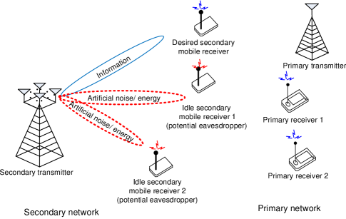
Figure 1: A CR network where $K=3$ secondary receivers (1 active and 2 idle receivers) share the same spectrum with $J=2$ primary receivers. The secondary transmitter conveys information and transfers power(/energy) to the $K$ secondary receivers simultaneously. The red dotted ellipsoids illustrate the dual use of artificial noise for providing security and facilitating efficient energy transfer to the secondary receivers.

We note that only one secondary receiver is selected for information transfer to reduce the multiple access interference leakage to the primary receivers [28]. On the other hand, the information signal of the desired secondary receiver is overheard by both the $K-1$ idle secondary receivers and the $J$ primary receivers. Hence, if the idle secondary receivers and the primary receivers are malicious, they may eavesdrop the signal of the selected secondary receiver, which has to be taken into account for resource allocation design to provide communication secrecy in the secondary network. Thus, for guaranteeing communication security, the secondary transmitter has to employ a resource allocation algorithm that accounts for this unfavourable scenario and treat both idle secondary receivers and primary receivers as potential eavesdroppers. We assume a frequency flat slow fading channel. The received signals at the desired secondary receiver, idle secondary receiver $k\in\{1,\ldots,K-1\}$, and primary receiver $j\in\{1,\ldots,J\}$ are given by, respectively,

$$y = \mathbf{h}^{H}\mathbf{x}+q\sqrt{P^{\mathrm{PU}}}d+z,$$ (1)

$$y_{k}^{\mathrm{Idle}} = \mathbf{g}_{k}^{H}\mathbf{x}+f_{k}\sqrt{P^{\mathrm{PU}}}d+z_{k},\,\forall k\in\{1,\ldots,K-1\},\,\mbox{and}$$ (2)

$$y_{j}^{\mathrm{PU}} = \mathbf{l}_{j}^{H}\mathbf{x}+t_{j}\sqrt{P^{\mathrm{PU}}}d+z_{\mathrm{PU}_{j}},\,\,\forall j\in\{1,\ldots,J\}.$$ (3)

Here, $\mathbf{x}\in\mathbb{C}^{N_{T}\times 1}$ denotes the symbol vector transmitted by the secondary transmitter. $\mathbf{h}^{H}\in\mathbb{C}^{1\times N_{T}}$, $\mathbf{g}_{k}^{H}\in\mathbb{C}^{1\times N_{T}}$, and $\mathbf{l}^{H}_{j}\in\mathbb{C}^{1\times N_{T}}$ are the channel vectors between the secondary transmitter and the desired secondary receiver, idle receiver (potential eavesdropper) $k$, and primary receiver (potential eavesdropper) $j$, respectively. $P^{\mathrm{PU}}$ and $d\in\mathbb{C}^{1\times 1}$ are the transmit power of the primary transmitter and the information signal intended for the primary receivers, respectively. $q\in\mathbb{C}^{1\times 1}$, $f_{k}\in\mathbb{C}^{1\times 1}$, and $t_{j}\in\mathbb{C}^{1\times 1}$ are the communication channels between the primary transmitter and desired secondary receiver, idle secondary receiver $k$, and primary receiver $j$, respectively. $z_{\mathrm{PU}_{j}}$ includes the joint effects of the thermal noise and the signal processing noise at primary receiver $j$ and is modelled as additive white Gaussian noise (AWGN) with zero mean and variance $\sigma_{\mathrm{PU}}^{2}$. $z$ and $z_{k}$ include the joint effects of thermal noise and signal processing noise at the desired secondary receiver and idle secondary receiver $k$, respectively, and are modeled as AWGN. Besides, the equivalent noises at the desired and idle secondary receivers, which capture the joint effect of the received interference from the primary transmitter, i.e., $q\sqrt{P^{\mathrm{PU}}}d$ and $f_{k}\sqrt{P^{\mathrm{PU}}}d$, thermal noise, and signal processing noise, are also modeled as AWGN with zero mean and variances $\sigma_{\mathrm{z}}^{2}$ and $\sigma_{\mathrm{z}_{k}}^{2}$, respectively.

Remark 1

In this paper, we assume that the primary network is a legacy system and the primary transmitter does not actively participate in transmit power control. Furthermore, we assume that the primary transmitter transmits a Gaussian signal and we focus on quasi-static fading channels such that all channel gains remain constant within the coherence time of the secondary system. These assumptions justify modelling the interference from the primary transmitter to the secondary receivers as additive white Gaussian noise with different powers for different secondary receivers. This model has been commonly adopted in the literature for resource allocation algorithm design [10, 28, 36].

To guarantee secure communication and to facilitate an efficient power transfer in the secondary system, artificial noise is generated at the secondary transmitter and is transmitted concurrently with the information signal. In particular, the transmit signal vector

$$\mathbf{x}=\underbrace{\mathbf{w}s}_{\mbox{desired signal}}+\underbrace{\mathbf{v}}_{\mbox{artificial noise}}$$ (4)

is adopted at the secondary transmitter, where $s\in\mathbb{C}^{1\times 1}$ and $\mathbf{w}\in\mathbb{C}^{N_{\mathrm{T}}\times 1}$ are the information bearing signal for the desired receiver and the corresponding beamforming vector, respectively. We assume without loss of generality that ${\cal E}\{\lvert s\rvert^{2}\}=1$. $\mathbf{v}\in\mathbb{C}^{N_{\mathrm{T}}\times 1}$ is the artificial noise vector generated by the secondary transmitter to combat the potential eavesdroppers. Specifically, $\mathbf{v}$ is modeled as a complex Gaussian random vector with mean $\mathbf{0}$ and covariance matrix $\mathbf{V}\in\mathbb{H}^{N_{\mathrm{T}}},\mathbf{V}\succeq\mathbf{0}$. We note that $\mathbf{w}$ and $\mathbf{V}$ have to be optimized such that the transmit signal of the secondary transmitter does not interfere severely with the primary users.

III Resource Allocation Problem Formulation

In this section, we define different quality of service (QoS) measures for the secondary CR network for providing wireless power transfer and secure communication to the secondary receivers while protecting the primary receivers. Then, we formulate three resource allocation problems reflecting three different system design objectives. For convenience, we define the following matrices: $\mathbf{H}=\mathbf{h}\mathbf{h}^{H}$, $\mathbf{G}_{k}=\mathbf{g}_{k}\mathbf{g}_{k}^{H},k\in\{1,\ldots,K-1\}$, and $\mathbf{L}_{j}=\mathbf{l}_{j}\mathbf{l}_{j}^{H},j\in\{1,\ldots,J\}$.

III-A System Achievable Rate and Secrecy Rate

Given perfect CSI at the receiver, the achievable rate (bit/s/Hz) between the secondary transmitter and the desired secondary receiver is given by

$$C=\log_{2}\Big{(}1+\Gamma\Big{)}\,\,\,\,\mbox{and}\,\,\,\,\Gamma=\frac{\mathbf{w}^{H}\mathbf{H}\mathbf{w}}{\operatorname{\mathrm{Tr}}(\mathbf{H}\mathbf{V})+\sigma_{\mathrm{z}}^{2}},$$ (5)

where $\Gamma$ is the received signal-to-interference-plus-noise ratio (SINR) at the desired secondary receiver. On the other hand, the achievable rates between the secondary transmitter and idle secondary receiver $k\in\{1,\ldots,K-1\}$ and primary receiver $j\in\{1,\ldots,J\}$ are given by

$$C^{\mathrm{Idle}}_{k} = \log_{2}\Big{(}1+\Gamma^{\mathrm{Idle}}_{k}\Big{)},\,\,\,\,\,\Gamma^{\mathrm{Idle}}_{k}=\frac{\mathbf{w}^{H}\mathbf{G}_{k}\mathbf{w}}{\operatorname{\mathrm{Tr}}(\mathbf{G}_{k}\mathbf{V})+\sigma_{\mathrm{z}_{k}}^{2}},\,\mbox{and}$$ (6)

$$C^{\mathrm{PU}}_{j} = \log_{2}\Big{(}1+\Gamma^{\mathrm{PU}}_{j}\Big{)},\,\,\,\,\,\Gamma^{\mathrm{PU}}_{j}=\frac{\mathbf{w}^{H}\mathbf{L}_{j}\mathbf{w}}{\operatorname{\mathrm{Tr}}(\mathbf{L}_{k}\mathbf{V})+\sigma_{\mathrm{PU}}^{2}},$$ (7)

respectively, where $\Gamma^{\mathrm{Idle}}_{k}$ and $\Gamma^{\mathrm{PU}}_{j}$ are the received SINRs at idle secondary receiver $k$ and primary receiver $j$, respectively. Since both the idle secondary receivers and the primary receivers are potential eavesdroppers, the maximum achievable secrecy rate between the secondary transmitter and the desired receiver is given by

$$C_{\mathrm{sec}}=\Big{[}C-\underset{\underset{j\in\{1,\ldots,J\}}{k\in\{1,\ldots,K-1\}}}{\max}\{C^{\mathrm{Idle}}_{k},C^{\mathrm{PU}}_{j}\}\Big{]}^{+}.$$ (8)

In the literature, the secrecy rate, i.e., (8), is commonly adopted as a QoS requirement for system design to ensure secure communication [26, 27]. In particular, $C_{\mathrm{sec}}$ quantifies the maximum achievable data rate at which a transmitter can reliably send secret information to the intended receiver such that the eavesdroppers are unable to decode the received signal [37] even if the eavesdroppers have unbounded computational capability.

III-B Energy Harvesting Efficiency

In the considered CR system, the secondary receivers harvest energy from the RF when they are idle to extend their lifetimes. The energy harvesting efficiency plays an important role in the system design of such secondary networks and has to be considered in the problem formulation. To this end, we define the energy harvesting efficiency in the secondary system as the ratio of the total power harvested at the idle secondary receivers and the total power radiated by the secondary transmitter. The total amount of energy harvested by the $K-1$ idle secondary receivers is modeled as

$$\mathrm{HP}(\mathbf{w},\mathbf{V})=\sum_{k=1}^{K-1}\eta_{k}\Big{(}\mathbf{w}^{H}\mathbf{G}_{k}\mathbf{w}+\operatorname{\mathrm{Tr}}(\mathbf{G}_{k}\mathbf{V})\Big{)},$$ (9)

where $\eta_{k}$ is a constant, $0\leq\eta_{k}\leq 1,\forall k$, which represents the RF energy conversion efficiency of idle secondary receiver $k$ in converting the received radio signal to electrical energy. We note that the power received at the secondary receivers from the primary transmitter and the AWGN power are neglected in (9) as we focus on the worst-case scenario for robust energy harvesting system design.

On the other hand, the power radiated by the transmitter can be expressed as

$$\mathrm{TP}(\mathbf{w},\mathbf{V})=\lVert\mathbf{w}\rVert^{2}+\operatorname{\mathrm{Tr}}(\mathbf{V}).$$ (10)

Thus, the energy harvesting efficiency of the considered secondary CR system is given by

$$\eta_{\mathrm{eff}}(\mathbf{w},\mathbf{V})=\frac{\mathrm{HP}(\mathbf{w},\mathbf{V})}{\mathrm{TP}(\mathbf{w},\mathbf{V})}.$$ (11)

III-C Interference Power Leakage-to-Transmit Power Ratio

In the considered CR network, the secondary receivers and the primary receivers share the same spectrum resource. However, the primary receivers are licensed users and thus the secondary transmitter is required to ensure the QoS of the primary receivers via a careful resource allocation design. Strong interference may impair the primary network when the secondary transmitter increases its transmit power for providing SWIPT services to the secondary receivers. As a result, the interference power leakage-to-transmit power ratio (IPTR) is an important performance measure for designing the secondary CR network and should be captured in the resource allocation algorithm design. To this end, we first define the total interference power received by the $J$ primary receivers as

$$\mathrm{IP}(\mathbf{w},\mathbf{V})=\sum_{j=1}^{J}\Big{(}\mathbf{w}^{H}\mathbf{L}_{j}\mathbf{w}+\operatorname{\mathrm{Tr}}(\mathbf{L}_{j}\mathbf{V})\Big{)}.$$ (12)

Thus, the IPTR of the considered secondary CR network is defined as

$$\mathrm{IP}_{\mathrm{ratio}}(\mathbf{w},\mathbf{V})=\frac{\mathrm{IP}(\mathbf{w},\mathbf{V})}{\mathrm{TP}(\mathbf{w},\mathbf{V})}.$$ (13)

III-D Channel State Information

In this paper, we focus on a Time Division Duplex (TDD) communication system with slowly time-varying channels. In practice, handshaking is performed between the secondary transmitter and the secondary receivers at the beginning of each scheduling slot. This allows the secondary transmitter to obtain the statuses and the QoS requirements of the secondary receivers. As a result, by exploiting the channel reciprocity, the downlink CSI of the secondary transmitter to the secondary receivers can be obtained by measuring the uplink training sequences embedded in the handshaking signals. Thus, we assume that the secondary-transmitter-to-secondary-receiver fading gains, $\mathbf{h}$ and $\mathbf{g}_{k},\forall k\in\{1,\ldots,K-1\}$, can be reliably estimated at the secondary transmitter at the beginning of each scheduling slot with negligible estimation error. Then, during the transmission, the desired secondary receiver is required to send positive acknowledgement (ACK) packets to inform the secondary transmitter of successful reception of the information packets. Hence, the transmitter is able to update the CSI estimate of the desired receiver frequently via the training sequences in each ACK packet. Therefore, perfect CSI for the secondary-transmitter-to-desired-secondary-receiver link, i.e., $\mathbf{h}$, is assumed over the entire transmission period. However, the remaining $K-1$ secondary receivers are idle and there is no interaction between them and the secondary transmitter after handshaking. As a result, the CSI of the idle secondary receivers becomes outdated during transmission. To capture the impact of the CSI imperfection and to isolate specific channel estimation methods from the resource allocation algorithm design, we adopt a deterministic model [40]–[43] for the resulting CSI uncertainty. In particular, the CSI of the link between the secondary transmitter and idle secondary receiver $k$ is modeled as

$$\mathbf{g}_{k} = \mathbf{\hat{g}}_{k}+\Delta\mathbf{g}_{k},\,\forall k\in\{1,\ldots,K-1\},\mbox{ and}$$ (14)

$${\Omega}_{k} \triangleq \Big{\{}\Delta\mathbf{g}_{k}\in\mathbb{C}^{N_{\mathrm{T}}\times 1}:\Delta\mathbf{g}_{k}^{H}\Delta\mathbf{g}_{k}\leq\varepsilon_{k}^{2}\Big{\}},\forall k,$$ (15)

where $\mathbf{\hat{g}}_{k}\in\mathbb{C}^{N_{\mathrm{T}}\times 1}$ is the CSI estimate available at the secondary transmitter at the beginning of a scheduling slot and $\Delta\mathbf{g}_{k}$ represents the unknown channel uncertainty due to the time varying nature of the channel during transmission. The continuous set ${\Omega}_{k}$ in (15) defines a Euclidean sphere and contains all possible channel uncertainties. Specifically, the radius $\varepsilon_{k}$ represents the size of the sphere and defines the uncertainty region of the CSI of idle secondary receiver (potential eavesdropper) $k$. In practice, the value of $\varepsilon_{k}^{2}$ depends on the coherence time of the associated channel and the duration of transmission.

Furthermore, to capture the imperfectness of the CSI of the primary receiver channels at the secondary transmitter, we adopt the same CSI error model as for the idle secondary receivers. In fact, the primary receivers are not directly interacting with the secondary transmitter. Besides, the primary receivers may be silent for non-negligible periods of time due to bursty data communication. As a result, the CSI of the primary receivers can be obtained only occasionally at the secondary transmitter when the primary receivers communicate with a primary transmitter. Hence, we model the CSI of the link between the secondary transmitter and primary receiver $j$ as

$$\mathbf{l}_{j} = \mathbf{\hat{l}}_{j}+\Delta\mathbf{l}_{j},\,\forall j\in\{1,\ldots,J\},\mbox{ and}$$ (16)

$${\Psi}_{j} \triangleq \Big{\{}\Delta\mathbf{l}_{j}\in\mathbb{C}^{N_{\mathrm{T}}\times 1}:\Delta\mathbf{l}_{j}^{H}\Delta\mathbf{l}_{j}\leq\upsilon_{j}^{2}\Big{\}},\forall j,$$ (17)

where $\mathbf{\hat{l}}_{j}$ is the estimate of the channel of primary receiver $j$ at the secondary transmitter and $\Delta\mathbf{l}_{j}$ denotes the associated channel uncertainty. ${\Psi}_{j}$ and $\upsilon_{j}^{2}$ in (17) define the continuous set of all possible channel uncertainties and the size of the uncertainty region of the estimated CSI of primary receiver $j$, respectively. We note that, in practice, the channel estimation qualities for primary receivers and secondary receivers at the secondary transmitter may be different which leads to different values for $\varepsilon_{k}$ and $\upsilon_{j}$.

III-E Optimization Problem Formulations

We first propose three problem formulations for single-objective system design for secure communication in the secondary CR network. In particular, each single-objective problem formulation considers one aspect of the system design. Then, we consider the three system design objectives jointly under the framework of multi-objective optimization. In particular, the adopted multi-objective optimization enables the design of a set of Pareto optimal resource allocation policies. The first problem formulation aims at maximizing the energy harvesting efficiency while providing secure communication in the secondary CR network. The problem formulation is as follows:

Problem 1

Energy Harvesting Efficiency Maximization:

$$\underset{\mathbf{V}\in\mathbb{H}^{N_{\mathrm{T}}},\mathbf{w}}{\operatorname{\mathrm{maximize}}}\,\,\,\,\min_{\Delta\mathbf{g}_{k}\in{\Omega}_{k}}\,\,\eta_{\mathrm{eff}}(\mathbf{w},\mathbf{V})$$

s.t. $$\mbox{C1: }\frac{\mathbf{w}^{H}\mathbf{H}\mathbf{w}}{\operatorname{\mathrm{Tr}}(\mathbf{H}\mathbf{V})+\sigma_{\mathrm{z}}^{2}}\geq\Gamma_{\mathrm{req}},$$ (18)

$$\mbox{C2: }\max_{\Delta\mathbf{g}_{k}\in{\Omega}_{k}}\frac{\mathbf{w}^{H}\mathbf{G}_{k}\mathbf{w}}{\operatorname{\mathrm{Tr}}(\mathbf{G}_{k}\mathbf{V})+\sigma_{\mathrm{z}_{k}}^{2}}\leq\Gamma_{\mathrm{tol}_{k}},\forall k\in\{1,\ldots,K-1\},$$

$$\mbox{C3: }\max_{\Delta\mathbf{l}_{j}\in{\Psi}_{j}}\,\,\frac{\mathbf{w}^{H}\mathbf{L}_{j}\mathbf{w}}{\operatorname{\mathrm{Tr}}(\mathbf{L}_{j}\mathbf{V})+\sigma_{\mathrm{PU}}^{2}}\leq\Gamma_{\mathrm{tol}_{j}}^{\mathrm{PU}},\forall j\in\{1,\ldots,J\},$$

$$\mbox{C4: }\lVert\mathbf{w}\rVert^{2}+\operatorname{\mathrm{Tr}}(\mathbf{V})\leq P_{\max},\quad\quad\mbox{C5:}\,\,\mathbf{V}\succeq\mathbf{0}.$$

The system objective in (III-E) is to maximize the worst case energy harvesting efficiency of the system for channel estimation errors $\Delta\mathbf{g}_{k}$ belonging to set $\Omega_{k}$. Constant $\Gamma_{\mathrm{req}}$ in C1 specifies the minimum required received SINR of the desired secondary receiver for information decoding. $\Gamma_{\mathrm{tol}_{k}},\forall k\in\{1,\ldots,K-1\}$, and $\Gamma_{\mathrm{tol}_{j}}^{\mathrm{PU}},\forall j\in\{1,\ldots,J\}$, in C2 and C3, respectively, are given system parameters which denote the maximum tolerable received SINRs at the potential eavesdroppers in the secondary network and the primary network, respectively. In practice, depending on the considered application, the system operator chooses the values of $\Gamma_{\mathrm{req}}$, $\Gamma_{\mathrm{tol}_{k}},\forall k\in\{1,\ldots,K-1\}$, and $\Gamma_{\mathrm{tol}_{j}}^{\mathrm{PU}},\forall j\in\{1,\ldots,J\}$, such that $\Gamma_{\mathrm{req}}\gg\Gamma_{\mathrm{tol}_{k}}>0$ and $\Gamma_{\mathrm{req}}\gg\Gamma_{\mathrm{tol}_{j}}^{\mathrm{PU}}>0$. In other words, the secrecy rate of the system is bounded below by $C_{\mathrm{sec}}\geq\log_{2}(1+\Gamma_{\mathrm{req}})-\log_{2}(1+\underset{k,j}{\max}\{\Gamma_{\mathrm{tol}_{k}},\Gamma_{\mathrm{tol}_{j}}^{\mathrm{PU}}\})>0$. We note that although $\Gamma_{\mathrm{req}}$, $\Gamma_{\mathrm{tol}_{k}}$, and $\Gamma_{\mathrm{tol}_{j}}^{\mathrm{PU}}$ in C1, C2, and C3, respectively, are not optimization variables in this paper, a balance between secrecy rate and system achievable rate can be struck by varying their values. $P_{\max}$ in C4 specifies the maximum transmit power in the power amplifier of the analog front-end of the secondary transmitter. C5 and $\mathbf{V}\in\mathbb{H}^{N_{\mathrm{T}}}$ are imposed since covariance matrix $\mathbf{V}$ has to be a positive semidefinite Hermitian matrix.

To facilitate the presentation and without loss of generality, we rewrite Problem 1 in (III-E) in the equivalent form [44]:

$$\underset{\mathbf{V}\in\mathbb{H}^{N_{\mathrm{T}}},\mathbf{w}}{\operatorname{\mathrm{minimize}}}\,\,\,\,\max_{\Delta\mathbf{g}_{k}\in{\Omega}_{k}}\,\,-\eta_{\mathrm{eff}}(\mathbf{w},\mathbf{V})$$

s.t. $$\mbox{C1 -- C5}.$$ (19)

The second system design objective is the minimization of the total transmit power of the secondary transmitter and can be mathematically formulated as:

Problem 2

Total Transmit Power Minimization:

$$\underset{\mathbf{V}\in\mathbb{H}^{N_{\mathrm{T}}},\mathbf{w}}{\operatorname{\mathrm{minimize}}}\,\,\,\,\mathrm{TP}(\mathbf{w},\mathbf{V})$$

s.t. $$\mbox{C1 -- C5}.$$ (20)

Problem 2 yields the minimum total transmit power of the secondary transmitter while ensuring that the QoS requirement on secure communication is satisfied. We note that Problem 2 does not take into account the energy harvesting capability of the idle secondary receivers and focuses only on the requirement of secure communication via constraints C1, C2, and C3. Besides, although transmit power minimization has been studied in the literature in different contexts [1, 45, 46], combining Problem 2 with the new Problems 1 and 3 (see below) offers new insights for the design of CR networks providing secure wireless information and power transfer to secondary receivers.

The third system design objective concerns the minimization of the worst case IPTR while providing secure communication in the secondary CR network. The problem formulation is given as:

Problem 3

Interference Power Leakage-to-Transmit Power Ratio Minimization:

$$\underset{\mathbf{V}\in\mathbb{H}^{N_{\mathrm{T}}},\mathbf{w}}{\operatorname{\mathrm{minimize}}}\,\,\,\,\max_{\Delta\mathbf{l}_{j}\in{\Psi}_{j}}\,\,\mathrm{IP}_{\mathrm{ratio}}(\mathbf{w},\mathbf{V})$$

s.t. $$\mbox{C1 -- C5}.$$ (21)

Remark 2

In (III-E) and (III-E), the maximization of the energy harvesting efficiency and the minimization of the IPTR are chosen as design objectives, respectively. Alternative design objectives are the maximization of the total harvested power, $\underset{\mathbf{V}\in\mathbb{H}^{N_{\mathrm{T}}},\mathbf{w}}{\operatorname{\mathrm{maximize}}}\,\,\underset{{\Delta\mathbf{g}_{k}\in{\Omega}_{k}}}{\min}\mathrm{HP}(\mathbf{w},\mathbf{V})$, and the minimization of the total interference power leakage, $\underset{\mathbf{V}\in\mathbb{H}^{N_{\mathrm{T}}},\mathbf{w}}{\operatorname{\mathrm{minimize}}}\,\,\,\,\underset{\Delta\mathbf{l}_{j}\in{\Psi}_{j}}{\max}\mathrm{IP}(\mathbf{w},\mathbf{V})$. We will show later that the maximization of the energy harvesting efficiency in (III-E) and the minimization of the IPTR in (III-E) subsume the total harvested power maximization and the total interference power leakage minimization as special cases, respectively. Please refer to Remark 7 for the solution of the total interference power leakage minimization and total harvested power maximization problems.

Remark 3

In fact, the optimization problem in (III-E) can be extended to the minimization of the maximum received interference leakage per primary receiver. However, such problem formulation does not facilitate the study of the trade-off between interference leakage, energy harvesting, and total transmit power as the system performance is always limited by those primary users which have strong channels with respect to the secondary transmitter.

In practice, the system design objectives in Problems $1$–$3$ are all desirable for the system operators of secondary CR networks in providing simultaneous power and secure information transfer. Yet, theses objectives are usually conflicting with each other and each objective focuses on only one aspect of the system. In the literature, multi-objective optimization has been proposed for studying the trade-off between conflicting system design objectives via the concept of Pareto optimality. For facilitating the following exposition, we denote the objective function and the optimal objective value for problem formulation $p\in\{1,2,3\}$ as $F_{p}(\mathbf{w},\mathbf{V})$ and $F_{p}^{*}$, respectively. We define a resource allocation policy which is Pareto optimal as:

Definition [47]: A resource allocation policy, $\{\mathbf{w,V}\}$, is Pareto optimal if and only if there does not exist another policy, $\{\mathbf{w^{\prime},V^{\prime}}\}$, such that $F_{i}(\mathbf{w}^{\prime},\mathbf{V}^{\prime})\leq F_{i}(\mathbf{w},\mathbf{V}),\forall i\in\{1,2,3\}$, and $F_{j}(\mathbf{w}^{\prime},\mathbf{V}^{\prime})<F_{j}(\mathbf{w},\mathbf{V})$ for at least one index $j\in\{1,2,3\}$.

The set of all Pareto optimal resource allocation polices is called the Pareto frontier or the Pareto optimal set. In this paper, we adopt the weighted Tchebycheff method [47] for investigating the trade-off between objective functions 1, 2, and 3. In particular, the weighted Tchebycheff method can provide the complete Pareto optimal set despite the non-convexity (if any) of the considered problems; it provides a necessary condition for Pareto optimality. The complete Pareto optimal set can be achieved by solving the following multi-objective problem:

Problem 4

Multi-Objective Optimization – Weighted Tchebycheff Method:

$$\underset{\mathbf{V}\in\mathbb{H}^{N_{\mathrm{T}}},\mathbf{w}}{\operatorname{\mathrm{minimize}}}\,\,\max_{p\in\{\,1,\,2,\,3\}}\,\,\Bigg{\{}\lambda_{p}\Big{(}\frac{F_{p}\big{(}\mathbf{w},\mathbf{V}\big{)}-F_{p}^{*}}{\lvert F_{p}^{*}\rvert}\Big{)}\Bigg{\}}$$

s.t. $$\hskip 8.53581pt\mbox{C1 -- C5},$$ (22)

In fact, by varying the values of $\lambda_{p}$, Problem 4 yields the complete Pareto optimal set [47, 48]. Besides, Problem 4 is a generalization of Problems 1, 2, and 3. In particular, Problem 4 is equivalent to Problem $p$ when $\lambda_{p}=1$ and $\lambda_{i}=0,\forall i\neq p$. For instance, if the secondary energy harvesting receivers do not require wireless power transfer from the secondary transmitter, without loss of generality, we can set $\lambda_{1}=0$ in Problem 4 to study the tradeoff between the remaining two system design objectives. In addition, this commonly adopted approach also provides a non-dimensional objective function, i.e., the unit of the objective function is normalized.

Remark 4

Finding the Pareto optimal set of the multi-objective optimization problem provides a set of Pareto optimal resource allocation policies. Then, depending on the preference of the system operator, a proper resource allocation policy can be selected from the set for implementation. We note that the resource allocation algorithm in [29] cannot be directly applied to the problems considered in this paper since it was designed for single-objective optimization, namely for the for minimization of the total transmit power.

Remark 5

Another possible problem formulation for the considered system model is to move some of the objective functions in (III-E), (III-E), and (III-E) to the set of constraints and constrain each of them by some constant. Then, by varying the constants, trade-offs between different objectives can be struck. However, in general, such a problem formulation does not reveal the Pareto optimal set due to the non-convexity of the problem.

IV Solution of the Optimization Problems

The optimization problems in (III-E), (III-E), and (III-E) are non-convex with respect to the optimization variables. In particular, the non-convexity arises from objective function 1, objective function 3, and constraint C1. In order to obtain tractable solutions for the problems, we recast Problems 1, 2, 3, and 4 as convex optimization problems by semidefinite programming (SDP) relaxation [49, 50] and study the tightness of the adopted relaxation in this section.

IV-A Semidefinite Programming Relaxation

To facilitate the SDP relaxation, we define

$$\mathbf{W}=\mathbf{w}\mathbf{w}^{H},\,\mathbf{W}=\frac{\overline{\mathbf{W}}}{\xi},\mathbf{V}=\frac{\overline{\mathbf{V}}}{\xi},\,\xi=\frac{1}{\operatorname{\mathrm{Tr}}({\mathbf{W}})+\operatorname{\mathrm{Tr}}({\mathbf{V}})},$$ (23)

and rewrite Problems 1 – 4 in terms of new optimization variables $\overline{\mathbf{W}}$, $\overline{\mathbf{V}}$, and $\xi$.

Transformed Problem 1

Energy Harvesting Efficiency Maximization:

$$\underset{\overline{\mathbf{V}},\overline{\mathbf{W}}\in\mathbb{H}^{N_{\mathrm{T}}},\xi}{\operatorname{\mathrm{minimize}}}\,\,\max_{\Delta\mathbf{g}_{k}\in{\Omega}_{k}}-\sum_{k=1}^{K-1}\eta_{k}\operatorname{\mathrm{Tr}}(\mathbf{G}_{k}(\overline{\mathbf{W}}+\overline{\mathbf{V}}))$$

s.t. $$\mbox{$\overline{\mbox{C1}}$:}\frac{\operatorname{\mathrm{Tr}}(\mathbf{H}\overline{\mathbf{W}})}{\operatorname{\mathrm{Tr}}(\mathbf{H}\overline{\mathbf{V}})+\sigma_{\mathrm{z}}^{2}\xi}\geq\Gamma_{\mathrm{req}},$$ (24)

$$\mbox{$\overline{\mbox{C2}}$: }\max_{\Delta\mathbf{g}_{k}\in{\Omega}_{k}}\frac{\operatorname{\mathrm{Tr}}(\mathbf{G}_{k}\overline{\mathbf{W}})}{\operatorname{\mathrm{Tr}}(\mathbf{G}_{k}\overline{\mathbf{V}})+\sigma_{\mathrm{z}_{k}}^{2}\xi}\leq\Gamma_{\mathrm{tol}_{k}},\forall k,$$

$$\mbox{$\overline{\mbox{C3}}$: }\max_{\Delta\mathbf{l}_{j}\in{\Psi}_{j}}\frac{\operatorname{\mathrm{Tr}}(\mathbf{L}_{j}\overline{\mathbf{W}})}{\operatorname{\mathrm{Tr}}(\mathbf{L}_{j}\overline{\mathbf{V}})+\sigma_{\mathrm{PU}}^{2}\xi}\leq\Gamma_{\mathrm{tol}_{j}}^{\mathrm{PU}},\forall j,$$

$$\mbox{$\overline{\mbox{C4}}$: }\operatorname{\mathrm{Tr}}(\overline{\mathbf{W}})+\operatorname{\mathrm{Tr}}(\overline{\mathbf{V}})\leq P_{\max}\xi,$$

$$\mbox{$\overline{\mbox{C5}}$:}\,\,\mathbf{\overline{W}},\mathbf{\overline{V}}\succeq\mathbf{0},\hskip 14.22636pt\mbox{$\overline{\mbox{C6}}$:}\,\,\xi\geq 0,$$

$$\mbox{$\overline{\mbox{C7}}$:}\,\,\operatorname{\mathrm{Tr}}(\overline{\mathbf{W}})+\operatorname{\mathrm{Tr}}(\overline{\mathbf{V}})=1,\,\,\mbox{$\overline{\mbox{C8}}$:}\,\,\operatorname{\mathrm{Rank}}(\mathbf{\overline{W}})=1,$$

where $\overline{\mathbf{W}}\succeq\mathbf{0}$, $\overline{\mathbf{W}}\in\mathbb{H}^{N_{\mathrm{T}}}$, and $\operatorname{\mathrm{Rank}}(\overline{\mathbf{W}})=1$ in (IV-A) are imposed to guarantee that $\overline{\mathbf{W}}=\xi\mathbf{w}\mathbf{w}^{H}$ after optimizing $\mathbf{\overline{W}}$.

Transformed Problem 2

Total Transmit Power Minimization:

$$\underset{\overline{\mathbf{V}},\mathbf{\overline{W}}\in\mathbb{H}^{N_{\mathrm{T}}},\xi}{\operatorname{\mathrm{minimize}}} \,\,\frac{1}{\xi}$$ (25)

$$\mbox{s.t. }\,\mbox{$\overline{\mbox{C1}}$ -- $\overline{\mbox{C8}}$}.$$

Transformed Problem 3

Interference Power Leakage-to-Transmit Power Ratio Minimization:

$$\underset{\overline{\mathbf{V}},\mathbf{\overline{W}}\in\mathbb{H}^{N_{\mathrm{T}}},\xi}{\operatorname{\mathrm{minimize}}} \,\,\max_{\Delta\mathbf{l}_{j}\in{\Psi}_{j}}\sum_{j=1}^{J}\operatorname{\mathrm{Tr}}(\mathbf{L}_{j}(\overline{\mathbf{W}}+\overline{\mathbf{V}}))$$ (26)

$$\mbox{s.t. }\,\mbox{$\overline{\mbox{C1}}$ -- $\overline{\mbox{C8}}$}.$$

Transformed Problem 4

Multi-Objective Optimization:

$$\hskip 28.45274pt\underset{\overline{\mathbf{V}},\mathbf{\overline{W}}\in\mathbb{H}^{N_{\mathrm{T}}},\xi,\tau}{\operatorname{\mathrm{minimize}}}\,\,\,\tau$$

$$\hskip 22.76228pt\mbox{s.t. }\,\mbox{$\overline{\mbox{C1}}$ -- $\overline{\mbox{C8}}$},$$

$$\mbox{$\overline{\mbox{C9}}$a: }\frac{\lambda_{1}}{\lvert F_{1}^{*}\rvert}(\overline{F_{1}}-F_{1}^{*})\leq\tau,\,\,\,\mbox{$\overline{\mbox{C9}}$b: }\frac{\lambda_{2}}{\lvert F_{2}^{*}\rvert}(\overline{F_{2}}-F_{2}^{*})\leq\tau,$$

$$\mbox{$\overline{\mbox{C9}}$c: }\frac{\lambda_{3}}{\lvert F_{3}^{*}\rvert}(\overline{F_{3}}-F_{3}^{*})\leq\tau,$$ (27)

where $\overline{F_{1}}=\underset{\Delta\mathbf{g}_{k}\in{\Omega}_{k}}{\min}-\sum_{k=1}^{K-1}\varepsilon_{k}\operatorname{\mathrm{Tr}}(\mathbf{G}_{k}(\overline{\mathbf{W}}+\overline{\mathbf{V}}))$, $\overline{F_{2}}=\frac{1}{\xi}$, $\overline{F_{3}}=\underset{\Delta\mathbf{l}_{j}\in{\Psi}_{j}}{\max}\sum_{j=1}^{J}\operatorname{\mathrm{Tr}}(\mathbf{L}_{j}(\overline{\mathbf{W}}+\overline{\mathbf{V}}))$, $\tau$ is an auxiliary optimization variable, and (IV-A) is the epigraph representation [44] of (III-E).

Proposition 1

The above transformed Problems (IV-A)–(IV-A) are equivalent to the original problems in (III-E)–(III-E), respectively. Specifically, we can recover the solutions of the original problems from the solutions of the transformed problems based on (23).

Proof:

Please refer to Appendix A. ∎

Since transformed Problem 4 is a generalization of transformed Problems 1, 2, and 3, we focus on the methodology for solving transformed Problem 4. In practice, the considered problems may be infeasible when the channels are in unfavourable conditions and/or the QoS requirements are too stringent. However, in the sequel, for studying the trade-off between different system design objectives and the design of different resource allocation schemes, we assume that the problem is always feasible.

First, we address constraints $\overline{\mbox{C2}}$, $\overline{\mbox{C3}}$, and $\overline{\mbox{C9}}$. We note that although these constraints are convex with respect to the optimization variables, they are semi-infinite constraints which are generally intractable. For facilitating the design of a tractable resource allocation algorithm, we introduce two auxiliary optimization variables $E_{k}^{\mathrm{SU}}$ and $I_{j}^{\mathrm{PU}}$ and rewrite transformed Problem 4 in (IV-A) as

$$\underset{\mathbf{\overline{W}},\overline{\mathbf{V}}\in\mathbb{H}^{N_{\mathrm{T}}},I_{j}^{\mathrm{PU}},E_{k}^{\mathrm{SU}},\xi,\tau,}{\operatorname{\mathrm{minimize}}}\,\,\,\tau$$

$$\mbox{s.t. }\,\mbox{$\overline{\mbox{C1}}$ -- $\overline{\mbox{C8}}$},$$

$$\mbox{$\overline{\mbox{C9}}$a: }\lambda_{1}\Big{(}\sum_{k=1}^{K-1}E_{k}^{\mathrm{SU}}-F_{1}^{*}\Big{)}\leq\tau\lvert F_{1}^{*}\rvert,$$

$$\mbox{$\overline{\mbox{C9}}$b: }\lambda_{2}(\overline{F_{2}}-F_{2}^{*})\leq\tau\lvert F_{2}^{*}\rvert,$$

$$\mbox{$\overline{\mbox{C9}}$c: }\lambda_{3}\Big{(}\sum_{j=1}^{J}I_{j}^{\mathrm{PU}}-F_{3}^{*}\Big{)}\leq\tau\lvert F_{3}^{*}\rvert,$$

$$\mbox{$\overline{\mbox{C10}}$: }E_{k}^{\mathrm{SU}}\geq\max_{\Delta\mathbf{g}_{k}\in{\Omega}_{k}}-\eta_{k}\operatorname{\mathrm{Tr}}(\mathbf{G}_{k}(\overline{\mathbf{W}}+\overline{\mathbf{V}})),\forall k,$$

$$\mbox{$\overline{\mbox{C11}}$: }I_{j}^{\mathrm{PU}}\geq\max_{\Delta\mathbf{l}_{j}\in{\Psi}_{j}}\operatorname{\mathrm{Tr}}(\mathbf{L}_{j}(\overline{\mathbf{W}}+\overline{\mathbf{V}})),\forall j.$$ (28)

In fact, the introduced auxiliary variables $E_{k}^{\mathrm{SU}}$ and $I_{j}^{\mathrm{PU}}$ decouple the original two nested semi-infinite constraints into two semi-infinite constraints and two affine constraints, i.e., $\overline{\mbox{C10}}$, $\overline{\mbox{C11}}$ and $\overline{\mbox{C9}}$a, $\overline{\mbox{C9}}$c, respectively. It can be verified that (IV-A) is equivalent to (26), i.e., constraints $\overline{\mbox{C10}}$ and $\overline{\mbox{C11}}$ are satisfied with equality for the optimal solution. Next, we transform constraints $\overline{\mbox{C2}}$, $\overline{\mbox{C3}}$, $\overline{\mbox{C10}}$, and $\overline{\mbox{C11}}$ into linear matrix inequalities (LMIs) using the following lemma:

Lemma 1 (S-Procedure [44])

Let a function $f_{m}(\mathbf{x}),m\in\{1,2\},\mathbf{x}\in\mathbb{C}^{N\times 1},$ be defined as

$$f_{m}(\mathbf{x})=\mathbf{x}^{H}\mathbf{A}_{m}\mathbf{x}+2\mathrm{Re}\{\mathbf{b}_{m}^{H}\mathbf{x}\}+c_{m},$$ (29)

where $\mathbf{A}_{m}\in\mathbb{H}^{N}$, $\mathbf{b}_{m}\in\mathbb{C}^{N\times 1}$, and $c_{m}\in\mathbb{R}$. Then, the implication $f_{1}(\mathbf{x})\leq 0\Rightarrow f_{2}(\mathbf{x})\leq 0$ holds if and only if there exists a $\delta\geq 0$ such that

$$\delta\begin{bmatrix}\mathbf{A}_{1}&\mathbf{b}_{1}\\ \mathbf{b}_{1}^{H}&c_{1}\\ \end{bmatrix}-\begin{bmatrix}\mathbf{A}_{2}&\mathbf{b}_{2}\\ \mathbf{b}_{2}^{H}&c_{2}\\ \end{bmatrix}\succeq\mathbf{0},$$ (30)

provided that there exists a point $\mathbf{\hat{x}}$ such that $f_{k}(\mathbf{\hat{x}})<0$.

Now, we apply Lemma 1 to constraint $\overline{\mbox{C2}}$. In particular, we substitute $\mathbf{g}_{k}=\mathbf{\hat{g}}_{k}+\Delta\mathbf{g}_{k}$ into constraint $\overline{\mbox{C2}}$. Therefore, the implication,

$$\Delta\mathbf{g}_{k}^{H}\Delta\mathbf{g}_{k}\leq\varepsilon_{k}^{2}$$ (31)

$$\Rightarrow\, \mbox{$\overline{\mbox{C2}}$: }0\geq\max_{\Delta\mathbf{g}_{k}\in{\Omega}_{k}}\Delta\mathbf{g}_{k}^{H}\big{(}\frac{\overline{\mathbf{W}}}{\Gamma_{\mathrm{tol}_{k}}}-\overline{\mathbf{V}}\big{)}\Delta\mathbf{g}_{k}$$

$$+2\mathrm{Re}\Big{\{}\mathbf{\hat{g}}_{k}^{H}\big{(}\frac{\overline{\mathbf{W}}}{\Gamma_{\mathrm{tol}_{k}}}-\overline{\mathbf{V}}\big{)}\Delta\mathbf{g}_{k}\Big{\}}+\mathbf{\hat{g}}_{k}^{H}\big{(}\frac{\overline{\mathbf{W}}}{\Gamma_{\mathrm{tol}_{k}}}-\overline{\mathbf{V}}\big{)}\mathbf{\hat{g}}_{k}-\xi\sigma_{\mathrm{z}_{k}}^{2},\forall k,$$

holds if and only if there exists a $\delta_{k}\geq 0$ such that the following LMI constraint holds:

$$\overline{\mbox{C2}} \mathbf{S}_{\mathrm{\overline{C2}}_{k}}(\overline{\mathbf{W}},\overline{\mathbf{V}},\xi,\delta_{k})$$: (32)

$$= \begin{bmatrix}\delta_{k}\mathbf{I}_{N_{\mathrm{T}}}+\overline{\mathbf{V}}-\frac{\overline{\mathbf{W}}}{\Gamma_{\mathrm{tol}_{k}}}&(\overline{\mathbf{V}}-\frac{\overline{\mathbf{W}}}{\Gamma_{\mathrm{tol}_{k}}})\mathbf{\hat{g}}_{k}\\ \mathbf{\hat{g}}_{k}^{H}(\overline{\mathbf{V}}-\frac{\overline{\mathbf{W}}}{\Gamma_{\mathrm{tol}_{k}}})&-\delta_{k}\varepsilon_{k}^{2}+\xi\sigma_{\mathrm{z}_{k}}^{2}+\mathbf{\hat{g}}_{k}^{H}(\overline{\mathbf{V}}-\frac{\overline{\mathbf{W}}}{\Gamma_{\mathrm{tol}_{k}}})\mathbf{\hat{g}}_{k}\\ \end{bmatrix}$$

$$= \begin{bmatrix}\delta_{k}\mathbf{I}_{N_{\mathrm{T}}}+\overline{\mathbf{V}}&\overline{\mathbf{V}}\mathbf{\hat{g}}_{k}\\ \mathbf{\hat{g}}_{k}^{H}\overline{\mathbf{V}}&-\delta_{k}\varepsilon_{k}^{2}+\xi\sigma_{\mathrm{z}_{k}}^{2}+\mathbf{\hat{g}}_{k}^{H}\overline{\mathbf{V}}\mathbf{\hat{g}}_{k}\\ \end{bmatrix}$$

$$- \frac{1}{\Gamma_{\mathrm{tol}_{k}}}\mathbf{U}_{\mathbf{g}_{k}}^{H}\overline{\mathbf{W}}\mathbf{U}_{\mathbf{g}_{k}}\succeq\mathbf{0},\forall k,$$

for $\delta_{k}\geq 0,k\in\{1,\ldots,K-1\}$ where $\mathbf{U}_{\mathbf{g}_{k}}=\Big{[}\mathbf{I}_{N_{\mathrm{T}}}\quad\mathbf{\hat{g}}_{k}\Big{]}$.

Similarly, we rewrite constraints $\overline{\mbox{C3}}$, $\overline{\mbox{C10}}$, and $\overline{\mbox{C11}}$ in the form of (29) which leads to

$$\overline{\mbox{C3}} 0\geq\max_{\Delta\mathbf{l}_{j}\in{\Psi}_{j}}\Delta\mathbf{l}_{j}^{H}\big{(}\frac{\overline{\mathbf{W}}}{\Gamma_{\mathrm{tol}_{j}}^{\mathrm{PU}}}-\overline{\mathbf{V}}\big{)}\Delta\mathbf{l}_{j}$$:

$$+2\mathrm{Re}\Big{\{}\mathbf{\hat{l}}_{j}^{H}\big{(}\frac{\overline{\mathbf{W}}}{\Gamma_{\mathrm{tol}_{j}}^{\mathrm{PU}}}-\overline{\mathbf{V}}\big{)}\Delta\mathbf{l}_{j}\Big{\}}+\mathbf{\hat{l}}_{j}^{H}\big{(}\frac{\overline{\mathbf{W}}}{\Gamma_{\mathrm{tol}_{j}}^{\mathrm{PU}}}-\overline{\mathbf{V}}\big{)}\mathbf{\hat{l}}_{j}-\xi\sigma_{\mathrm{PU}}^{2},\forall k,$$

$$\overline{\mbox{C10}} 0\geq\max_{\Delta\mathbf{g}_{k}\in{\Omega}_{k}}-\eta_{k}\Big{\{}\Delta\mathbf{g}_{k}^{H}\big{(}\overline{\mathbf{W}}+\overline{\mathbf{V}}\big{)}\Delta\mathbf{g}_{k}$$:

$$+2\mathrm{Re}\Big{\{}\mathbf{\hat{g}}_{k}^{H}\big{(}\overline{\mathbf{W}}+\overline{\mathbf{V}}\big{)}\Delta\mathbf{g}_{k}\Big{\}}+\mathbf{\hat{g}}_{k}^{H}\big{(}\overline{\mathbf{W}}+\overline{\mathbf{V}}\big{)}\mathbf{\hat{g}}_{k}\Big{\}}-E_{k}^{\mathrm{SU}},\forall k,\,\mbox{and}$$

$$\overline{\mbox{C11}} 0\geq\max_{\Delta\mathbf{l}_{j}\in{\Psi}_{j}}\Delta\mathbf{l}_{j}^{H}\big{(}\overline{\mathbf{W}}+\overline{\mathbf{V}}\big{)}\Delta\mathbf{l}_{j}$$:

$$+2\mathrm{Re}\Big{\{}\mathbf{\hat{l}}_{j}^{H}\big{(}\overline{\mathbf{W}}+\overline{\mathbf{V}}\big{)}\Delta\mathbf{l}_{j}\Big{\}}+\mathbf{\hat{l}}_{j}^{H}\big{(}\overline{\mathbf{W}}+\overline{\mathbf{V}}\big{)}\mathbf{\hat{l}}_{j}-I_{j}^{\mathrm{PU}},\forall j,$$

respectively.

$$\hskip 85.35826pt\underset{\mathbf{\Theta}}{\operatorname{\mathrm{minimize}}}\,\,\,\tau$$

$$\hskip 5.69046pt\mbox{s.t. }\,\mbox{$\overline{\mbox{C1}}$, $\overline{\mbox{C4}}$ -- $\overline{\mbox{C7}}$},\,\mbox{$\overline{\mbox{C8}}$: }\operatorname{\mathrm{Rank}}(\overline{\mathbf{W}})=1,\,\mbox{$\overline{\mbox{C9}}$a},\,\mbox{$\overline{\mbox{C9}}$b},\,\mbox{$\overline{\mbox{C9}}$c},$$

$$\mbox{$\overline{\mbox{C2}}$: }\mathbf{S}_{\mathrm{\overline{C2}}_{k}}(\overline{\mathbf{W}},\overline{\mathbf{V}},\xi,\delta_{k})\succeq\mathbf{0},\forall k,\hskip 31.2982pt\mbox{$\overline{\mbox{C3}}$: }\mathbf{S}_{\mathrm{\overline{C3}}_{j}}(\overline{\mathbf{W}},\overline{\mathbf{V}},\xi,\gamma_{j})\succeq\mathbf{0},\forall j,$$

$$\mbox{$\overline{\mbox{C10}}$: }\mathbf{S}_{\mathrm{\overline{C10}}_{k}}(\overline{\mathbf{W}},\overline{\mathbf{V}},E_{k}^{\mathrm{SU}},\varphi_{k})\succeq\mathbf{0},\forall k,\hskip 8.53581pt\mbox{$\overline{\mbox{C11}}$: }\mathbf{S}_{\mathrm{\overline{C11}}_{j}}(\overline{\mathbf{W}},\overline{\mathbf{V}},I_{j}^{\mathrm{PU}},\omega_{j})\succeq\mathbf{0},\forall j,$$

$$\mbox{$\overline{\mbox{C12}}$: }\delta_{k}\geq 0,\forall k,\,\,\,\,\,\,\,\,\,\,\,\,\mbox{$\overline{\mbox{C13}}$: }\gamma_{j}\geq 0,\forall j,\,\,\,\,\,\mbox{$\overline{\mbox{C14}}$: }\varphi_{k}\geq 0,\forall k,\,\,\,\,\,\,\,\,\mbox{$\overline{\mbox{C15}}$: }\omega_{j}\geq 0,\forall j,$$ (39)

By using Lemma 1, constraint $\overline{\mbox{C3}}$, $\overline{\mbox{C10}}$, and $\overline{\mbox{C11}}$ can be equivalently written as

$$\mbox{$\overline{\mbox{C3}}$: }\mathbf{S}_{\mathrm{\overline{C3}}_{j}}(\overline{\mathbf{W}},\overline{\mathbf{V}},\xi,\gamma_{j})$$

$$= \begin{bmatrix}\gamma_{j}\mathbf{I}_{N_{\mathrm{T}}}+\overline{\mathbf{V}}&\overline{\mathbf{V}}\mathbf{\hat{l}}_{j}\\ \mathbf{\hat{l}}_{j}^{H}\overline{\mathbf{V}}&-\gamma_{j}\upsilon_{j}^{2}+\xi\sigma_{\mathrm{PU}}^{2}+\mathbf{\hat{l}}_{j}^{H}\overline{\mathbf{V}}\mathbf{\hat{l}}_{j}\\ \end{bmatrix}$$

$$- \frac{\mathbf{U}_{\mathbf{l}_{j}}^{H}\overline{\mathbf{W}}\mathbf{U}_{\mathbf{l}_{j}}}{\Gamma_{\mathrm{tol}_{j}}^{\mathrm{PU}}}\succeq\mathbf{0},\forall j,$$

$$\mbox{$\overline{\mbox{C10}}$: }\mathbf{S}_{\mathrm{\overline{C10}}_{k}}(\overline{\mathbf{W}},\overline{\mathbf{V}},E_{k}^{\mathrm{SU}},\varphi_{k})$$

$$= \begin{bmatrix}\varphi_{k}\mathbf{I}_{N_{\mathrm{T}}}+\overline{\mathbf{V}}&\overline{\mathbf{V}}\mathbf{\hat{g}}_{k}\\ \mathbf{\hat{g}}_{h}^{H}\overline{\mathbf{V}}&-\varphi_{k}\varepsilon_{k}^{2}+\frac{E_{k}^{\mathrm{SU}}}{\eta_{k}}+\mathbf{\hat{g}}_{k}^{H}\overline{\mathbf{V}}\mathbf{\hat{g}}_{k}\\ \end{bmatrix}$$

$$+ \mathbf{U}_{\mathbf{g}_{k}}^{H}\overline{\mathbf{W}}\mathbf{U}_{\mathbf{g}_{k}}\succeq\mathbf{0},\forall k,$$

$$\mbox{$\overline{\mbox{C11}}$: }\mathbf{S}_{\mathrm{\overline{C11}}_{j}}(\overline{\mathbf{W}},\overline{\mathbf{V}},I_{j}^{\mathrm{PU}},\omega_{j})$$

$$= \begin{bmatrix}\omega_{j}\mathbf{I}_{N_{\mathrm{T}}}-\overline{\mathbf{V}}&-\overline{\mathbf{V}}\mathbf{\hat{l}}_{j}\\ -\mathbf{\hat{l}}_{j}^{H}\overline{\mathbf{V}}&-\omega_{j}\upsilon_{j}^{2}+I_{j}^{\mathrm{PU}}-\mathbf{\hat{l}}_{j}^{H}\overline{\mathbf{V}}\mathbf{\hat{l}}_{j}\\ \end{bmatrix}$$

$$- \mathbf{U}_{\mathbf{l}_{j}}^{H}\overline{\mathbf{W}}\mathbf{U}_{\mathbf{l}_{j}}\succeq\mathbf{0},\forall j,$$ (38)

respectively, with $\mathbf{U}_{\mathbf{l}_{j}}=\Big{[}\mathbf{I}_{N_{\mathrm{T}}}\quad\mathbf{\hat{l}}_{j}\Big{]}$ and new auxiliary optimization variables $\gamma_{j}\geq 0,j\in\{1,\ldots,J\},$ $\varphi_{k}\geq 0,k\in\{1,\ldots,K-1\},$ and $\omega_{j}\geq 0,j\in\{1,\ldots,J\}$. We note that now constraints $\mbox{$\overline{\mbox{C2}}$},\mbox{$\overline{\mbox{C3}}$},\mbox{$\overline{\mbox{C10}}$}$, and $\overline{\mbox{C11}}$ involve only a finite number of convex constraints which facilitates an efficient resource allocation algorithm design. As a result, we obtain the following equivalent optimization problem on the top of this page in (IV-A), where $\mathbf{\Theta}\triangleq\{\mathbf{I}^{\mathrm{PU}},\mathbf{E}^{\mathrm{SU}},\xi,\tau,\boldsymbol{\gamma},\boldsymbol{\delta},\boldsymbol{\varphi},\boldsymbol{\omega},\overline{\mathbf{V}}\in\mathbb{H}^{N_{\mathrm{T}}},\mathbf{\overline{W}}\in\mathbb{H}^{N_{\mathrm{T}}}\}$ denotes the set of optimization variables after transformation; $\mathbf{I}^{\mathrm{PU}}$ and $\mathbf{E}^{\mathrm{SU}}$ are auxiliary variable vectors with elements ${I}_{j}^{\mathrm{PU}},\forall j\in\{1,\ldots,J\},$ and ${E}_{k}^{\mathrm{SU}},\forall k\in\{1,\ldots,K-1\}$, respectively; $\boldsymbol{\delta},\boldsymbol{\gamma},\boldsymbol{\varphi}$, and $\boldsymbol{\omega}$ are auxiliary optimization variable vectors with elements $\delta_{k},\gamma_{j},\varphi_{k}$, and $\omega_{j}\geq 0$ connected to the constraints in (32)–(IV-A), respectively.

The remaining non-convexity of problem (IV-A) is due to the combinatorial rank constraint in $\overline{\mbox{C8}}$ on the beamforming matrix $\overline{\mathbf{W}}$. In fact, by relaxing constraint $\mbox{$\overline{\mbox{C8}}$: }\operatorname{\mathrm{Rank}}(\overline{\mathbf{W}})=1$, i.e., removing it from (IV-A), the considered problem is a convex SDP and can be solved efficiently by numerical solvers such as SeDuMi [51] and CVX [52]. Besides, if the obtained solution for the relaxed SDP problem admits a rank-one matrix $\overline{\mathbf{W}}$, i.e., $\operatorname{\mathrm{Rank}}(\overline{\mathbf{W}})=1$, then it is the optimal solution of the original problem. In general, the adopted SDP relaxation may not yield a rank-one solution and the result of the relaxed problem serves as a performance upper bound for the original problem. Nevertheless, in the following, we show that there always exists an optimal solution for the relaxed problem with $\operatorname{\mathrm{Rank}}(\mathbf{\overline{W}})=1$. In particular, the optimal solution of the relaxed version of (IV-A) with $\operatorname{\mathrm{Rank}}(\mathbf{\overline{W}})=1$ can be obtained from the solution of the dual problem of the SDP relaxed version of (IV-A). In other words, we can obtain the global optimal solutions of non-convex Problems 1, 2, 3, and 4. Furthermore, we propose two suboptimal resource allocation schemes which do not require the solution of the dual problem of the SDP relaxed problem.

IV-B Optimality Condition for SDP Relaxation

In this subsection, we first reveal the tightness of the proposed SDP relaxation. The existence of a rank-one solution matrix $\overline{\mathbf{W}}$ for the relaxed SDP version of transformed Problem 4 is summarized in the following theorem which is based on [30, Proposition 4.1].

Theorem 1

Suppose the optimal solution for the SDP relaxed version of (IV-A) is denoted as $\mathbf{\Lambda}^{*}\triangleq\{\mathbf{I}^{\mathrm{PU}*},\mathbf{E}^{\mathrm{SU}*},\xi^{*},\tau^{*},\boldsymbol{\gamma^{*}},\boldsymbol{\delta^{*}},\boldsymbol{\varphi^{*}},\boldsymbol{\omega^{*}},\overline{\mathbf{V}}^{*},\mathbf{\overline{W}}^{*}\}$ and $\operatorname{\mathrm{Rank}}(\overline{\mathbf{W}}^{*})>1$. Then, there exists a feasible solution for the SDP relaxed version of (IV-A), denoted as $\mathbf{\widetilde{\Lambda}}\triangleq\{\mathbf{\widetilde{I}}^{\mathrm{PU}},\mathbf{\widetilde{E}}^{\mathrm{SU}},\widetilde{\xi},\widetilde{\tau},\boldsymbol{\widetilde{\gamma}},\boldsymbol{\widetilde{\delta}},\boldsymbol{\widetilde{\varphi}},\boldsymbol{\widetilde{\omega}},$ ${\mathbf{\widetilde{V}}},\mathbf{{\widetilde{W}}}\}$, which not only achieves the same objective value as $\mathbf{\Lambda}^{*}$, but also admits a rank-one matrix $\mathbf{\widetilde{W}}$, i.e., $\operatorname{\mathrm{Rank}}(\mathbf{\widetilde{W}})=1$. The solution $\mathbf{\widetilde{\Lambda}}$ can be constructed exploiting $\mathbf{\Lambda}^{*}$ and the solution of the dual problem of the relaxed version of (IV-A).

Proof:

Please refer to Appendix B for the proof of Theorem 1 and the method for constructing the optimal solution. ∎

Since there always exists an achievable optimal solution with a rank-one beamforming matrix $\mathbf{\widetilde{W}}$, the global optimum of (IV-A) can be obtained despite the SDP relaxation. By utilizing Theorem 1, we specify the optimal solution of transformed Problems $1$–$3$ in the following corollary.

$$\hskip 128.0374pt\underset{\mathbf{\Theta}_{\mathrm{sub}}}{\operatorname{\mathrm{minimize}}}\,\,\tau$$

$$\mbox{s.t.}\hskip 71.13188pt\mbox{$\overline{\mbox{C9}}$a},\,\,\mbox{$\overline{\mbox{C9}}$b},\,\,\mbox{$\overline{\mbox{C9}}$c},\mbox{$\overline{\mbox{C12}}$}-\mbox{$\overline{\mbox{C15}}$},$$

$$\mbox{$\overline{\mbox{C1}}$: }\frac{P_{b}\operatorname{\mathrm{Tr}}(\mathbf{H}\overline{\mathbf{W}}_{\mathrm{sub}})}{\operatorname{\mathrm{Tr}}(\mathbf{H}\overline{\mathbf{V}})+\sigma_{\mathrm{z}}^{2}}\geq\Gamma_{\mathrm{req}},\,\,\mbox{$\overline{\mbox{C2}}$: }\mathbf{S}_{\mathrm{\overline{C2}}_{k}}(P_{b}\overline{\mathbf{W}}_{\mathrm{sub}},\overline{\mathbf{V}},\xi,\delta_{k})\succeq\mathbf{0},\forall k,$$

$$\mbox{$\overline{\mbox{C3}}$: }\mathbf{S}_{\mathrm{\overline{C3}}_{j}}(P_{b}\overline{\mathbf{W}}_{\mathrm{sub}},\overline{\mathbf{V}},\xi,\gamma_{j})\succeq\mathbf{0},\forall j,\quad\mbox{$\overline{\mbox{C4}}$: }P_{b}\operatorname{\mathrm{Tr}}(\overline{\mathbf{W}}_{\mathrm{sub}})+\operatorname{\mathrm{Tr}}(\overline{\mathbf{V}})\leq P_{\max}\xi,$$

$$\mbox{$\overline{\mbox{C5}}$:}\,\,P_{b}\geq 0,\mathbf{\overline{V}}\succeq\mathbf{0},\quad\mbox{$\overline{\mbox{C6}}$:}\,\,\xi\geq 0,\quad\mbox{$\overline{\mbox{C7}}$:}\,\,P_{b}\operatorname{\mathrm{Tr}}(\overline{\mathbf{W}}_{\mathrm{sub}})+\operatorname{\mathrm{Tr}}(\overline{\mathbf{V}})=1,\quad$$

$$\mbox{$\overline{\mbox{C10}}$: }\mathbf{S}_{\mathrm{\overline{C10}}_{k}}(P_{b}\overline{\mathbf{W}}_{\mathrm{sub}},\overline{\mathbf{V}},{E}^{\mathrm{SU}}_{k},\varphi_{k})\succeq\mathbf{0},\forall k,\quad\mbox{$\overline{\mbox{C11}}$: }\mathbf{S}_{\mathrm{\overline{C11}}_{j}}(P_{b}\overline{\mathbf{W}}_{\mathrm{sub}},\overline{\mathbf{V}},{I}^{\mathrm{PU}}_{j},\omega_{j})\succeq\mathbf{0},\forall j,$$ (41)

Corollary 1

Transformed Problems $1$–$3$ can be solved optimally by applying SDP relaxation and the solution of each problem can be obtained with the method provided in the proof of Theorem $1$. In particular, Problem $p$ can be solved by solving Problem 4 with $\lambda_{p}=1$, $\lambda_{i}=0,\forall i\neq p$, $i\in\{1,2,3\}$, and setting $F_{p}^{*},\forall p\in\{1,2,3\},$ to any non-negative and finite constant.

Remark 6

The computational complexity of the proposed optimal algorithm with respect to the numbers of secondary users $K$, the number of primary users $J$, and transmit antennas $N_{\mathrm{T}}$ at the secondary transmitter can be characterized as

$$\operatorname{\cal O}\Bigg{(}\Big{(}\sqrt{2N_{\mathrm{T}}}\log\big{(}\frac{1}{\kappa}\big{)}\Big{)}\Big{(}(2K+2J)(2N_{\mathrm{T}})^{3}$$

$$+(2N_{\mathrm{T}})^{2}(2K+2J)^{2}+(2K+2J)^{3}\Big{)}\Bigg{)}$$ (40)

for a given solution accuracy $\kappa>0$, where $\operatorname{\cal O}(\cdot)$ is the big-O notation. We note that polynomial time computational complexity algorithms are considered to be fast algorithms in the literature [53, Chapter 34] and are desirable for real time implementation. Besides, the computational complexity can be further reduced by adopting a tailor made interior point method [54, 55]. Also, we would like to emphasize that in practice, $\lambda_{1},\lambda_{2},$ and $\lambda_{3}$ are given parameters and thus we only need to compute one point of the trade-off region.

IV-C Suboptimal Resource Allocation Schemes

As discussed in Appendix B, constructing the optimal solution $\mathbf{\widetilde{\Lambda}}$ with $\operatorname{\mathrm{Rank}}(\mathbf{\widetilde{W}})=1$ requires the solution of the dual problem of problem (IV-A) as the Lagrange multiplier matrix $\mathbf{Y}^{*}$ is needed in (50). Nevertheless, $\mathbf{Y}^{*}$ may not be provided by some numerical solvers and thus the construction of a rank-one solution matrix $\mathbf{\widetilde{W}}$ may not be possible. In the following, we propose two suboptimal resource allocation schemes based on the solution of the primal problem of the relaxed version of (IV-A) which do not require knowledge of $\mathbf{Y}^{*}$ when $\operatorname{\mathrm{Rank}}(\overline{\mathbf{W}}^{*})>1$.

IV-C1 Suboptimal Resource Allocation Scheme 1

The first proposed suboptimal resource allocation scheme is a hybrid scheme and is based on the solution of the relaxed version of (IV-A). We first solve (IV-A) by SDP relaxation. If the solution admits a rank-one $\overline{\mathbf{W}}$, then the global optimal solution of (IV-A) is obtained. Otherwise, we construct a suboptimal beamforming matrix $\overline{\mathbf{W}}_{\mathrm{sub}}$. Suppose $\overline{\mathbf{W}}$ is a matrix with rank $N$. Then $\overline{\mathbf{W}}$ can be written as $\overline{\mathbf{W}}=\sum_{t=1}^{N}\vartheta_{t}\mathbf{e}_{t}\mathbf{e}^{H}_{t}$, where $\vartheta_{t}$ and $\mathbf{e}_{t}\in\mathbb{C}^{N_{\mathrm{T}}\times 1}$ are the descending eigenvalues, i.e., $\vartheta_{1}\geq\vartheta_{2}\geq,\ldots,\geq\vartheta_{t},\ldots,\geq\vartheta_{N}$, and eigenvectors associated with $\overline{\mathbf{W}}$, respectively. Now, we introduce the suboptimal beamforming vector $\overline{\mathbf{w}}_{\mathrm{sub}}=\mathbf{e}_{1}$ such that $\overline{\mathbf{W}}_{\mathrm{sub}}=\overline{\mathbf{w}}_{\mathrm{sub}}\overline{\mathbf{w}}_{\mathrm{sub}}^{H}$. Then, we define a scalar optimization variable $P_{b}$ which controls the power of the suboptimal beamforming matrix. As a result, a new optimization problem is then given by (IV-B) on the top of this page, where $\mathbf{\Theta}_{\mathrm{sub}}\triangleq\{P_{b},\mathbf{I}^{\mathrm{PU}},\mathbf{E}^{\mathrm{SU}},\xi,\tau,\boldsymbol{\gamma},\boldsymbol{\delta},\boldsymbol{\varphi},\boldsymbol{\omega},\overline{\mathbf{V}}\in\mathbb{H}^{N_{\mathrm{T}}}\}$ is the new set of optimization variables for suboptimal resource allocation scheme 1. The problem formulation in (IV-B) is jointly convex with respect to the optimization variables and can be solved by using efficient numerical solvers. Besides, the solution of (IV-B) satisfies the constraints of (IV-A), thus the solution of (IV-B) serves as a suboptimal solution for (IV-A) since the beamforming matrix $\overline{\mathbf{W}}_{\mathrm{sub}}$ is fixed which leads to reduced degrees of freedom for resource allocation.

IV-C2 Suboptimal Resource Allocation Scheme 2

The second proposed suboptimal resource allocation scheme is also a hybrid scheme. It adopts a similar approach to solve the problem as suboptimal resource allocation scheme $1$, except for the choice of the suboptimal beamforming matrix $\overline{\mathbf{W}}_{\mathrm{sub}}$ when $\operatorname{\mathrm{Rank}}(\overline{\mathbf{W}}^{*})>1$. Here, the choice of beamforming matrix $\overline{\mathbf{W}}_{\mathrm{sub}}$ is based on the rank-one Gaussian randomization scheme [56]. Specifically, we calculate the eigenvalue decomposition of $\overline{\mathbf{W}}^{*}=\mathbf{U}\mathbf{\Sigma}\mathbf{U}^{H}$, where $\mathbf{U}=\Big{[}\mathbf{e}_{1}\ldots\mathbf{e}_{N}\Big{]}$ and $\mathbf{\Sigma}=\operatorname{\mathrm{diag}}\big{(}{\vartheta_{1}},\ldots,{\vartheta_{N}}\big{)}$ are an $N_{\mathrm{T}}\times N_{\mathrm{T}}$ unitary matrix and a diagonal matrix, respectively. Then, we adopt the suboptimal beamforming vector $\overline{\mathbf{w}}_{\mathrm{sub}}=\mathbf{U}\mathbf{\Sigma}^{1/2}\mathbf{r},\overline{\mathbf{W}}_{\mathrm{sub}}=P_{b}\overline{\mathbf{w}}_{\mathrm{sub}}\overline{\mathbf{w}}_{\mathrm{sub}}^{H}$, where $\mathbf{r}\in{\mathbb{C}}^{N_{\mathrm{T}}\times 1}$ and $\mathbf{r}\sim{\cal CN}(\mathbf{0},\mathbf{I}_{N_{\mathrm{T}}})$. Subsequently, we follow the same approach as in (IV-B) for optimizing $\mathbf{\Theta}_{\mathrm{sub}}$ and obtain a suboptimal rank-one solution $P_{b}\overline{\mathbf{W}}_{\mathrm{sub}}$. We note that suboptimal resource allocation scheme $2$ provides flexibility for trading computational complexity and system performance which is not offered by scheme $1$. In fact, by executing scheme $2$ repeatedly for different Gaussian distributed random vectors $\mathbf{r}$, the performance of scheme $2$ can be improved by selecting the best $\overline{\mathbf{w}}_{\mathrm{sub}}=\mathbf{U}\mathbf{\Sigma}^{1/2}\mathbf{r}$ over different trials.

Remark 7

We note that the solution of the total received interference power minimization ($\underset{\mathbf{V}\in\mathbb{H}^{N_{\mathrm{T}}},\mathbf{w}}{\operatorname{\mathrm{minimize}}}\,\underset{\Delta\mathbf{l}_{j}\in{\Psi}_{j}}{\max}$ $\mathrm{IP}(\mathbf{w},\mathbf{V})$) and total harvested power maximization ($\underset{\mathbf{V}\in\mathbb{H}^{N_{\mathrm{T}}},\mathbf{w}}{\operatorname{\mathrm{maximize}}}\,\underset{{\Delta\mathbf{g}_{k}\in{\Omega}_{k}}}{\min}\mathrm{HP}(\mathbf{w},\mathbf{V})$) problems can be obtained by applying Corollary 1 and solving Problem 4 after setting $\zeta=1$ and removing constraint $\overline{\mbox{C7}}$.

V Results

We evaluate the system performance of the proposed resource allocation schemes using simulations. The important simulation parameters are summarized in Table I. A reference distance of $2$ meters for the path loss model is selected. There are $K$ receivers uniformly distributed between the reference distance and the maximum service distance of $20$ meters in the secondary network. Besides, we assume that the primary transmitter is $40$ meters away from the secondary transmitter. In particular, there are $J$ primary receivers uniformly distributed between $20$ meters and $40$ from the secondary transmitter, cf. Figure 2. Because of path loss and channel fading, different secondary receivers experience different interference powers from the primary transmitter. To facilitate the presentation, in the sequel, we define the normalized maximum channel estimation errors of primary receiver $j$ and idle secondary receiver $k$ as $\sigma_{\mathrm{PU}_{j}}^{2}=\frac{\upsilon^{2}_{j}}{\lVert\mathbf{l}_{j}\rVert^{2}}$ and $\sigma_{\mathrm{SU}_{k}}^{2}=\frac{\varepsilon^{2}_{k}}{\lVert\mathbf{g}_{k}\rVert^{2}}$, respectively, with $\sigma_{\mathrm{PU}_{a}}^{2}=\sigma_{\mathrm{PU}_{b}}^{2},\forall a,b\in\{1,\ldots,J\}$, for all primary receivers and $\sigma_{\mathrm{SU}_{c}}^{2}=\sigma_{\mathrm{SU}_{d}}^{2},\forall c,d\in\{1,\ldots,K-1\}$, for all secondary receivers, respectively. Unless specified otherwise, we assume normalized maximum channel estimation errors of idle secondary receiver $k$ and primary receiver $j$ of $\sigma_{\mathrm{SU}_{k}}^{2}=0.01,\sigma_{\mathrm{PU}_{j}}^{2}=0.05,\forall k,j$. Besides, we study the trade-off between the different objective functions via the solution of Problem 4 for two cases. In particular, in Case I, we study the trade-off between the objective functions for total harvested power maximization, total interference power leakage minimization, and total transmit power minimization, cf. Remark 2 and Remark 7; in Case II, we study the trade-off between the objective functions for energy harvesting efficiency maximization, average IPTR minimization, and average total transmit power minimization. The average system performance shown in the following sections is obtained by averaging over different realizations of both path loss and multipath fading.

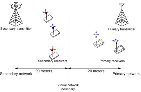
Figure 2: CR SWIPT network simulation topology.

TABLE I: System parameters.

Carrier center frequency	915 MHz
Path loss model	TGn path loss model E [57]
Multipath fading distribution	Rician fading with Rician factor $3$ dB
Total noise variance, $\sigma_{\mathrm{s}}^{2}$	$-23$ dBm
Transmit antenna gain	$10$ dBi
Number of transmit antennas at the secondary transmitter, $N_{\mathrm{T}}$	$8$
Max. transmit power allowance at the secondary transmitter, $P_{l}^{T_{\max}}$	$30$ dBm
Min. required SINR of the desired secondary receiver, $\Gamma_{\mathrm{req}}$	$20$ dB
Max. tolerable SINR at the potential eavesdroppers, $\Gamma_{\mathrm{tol}_{k}}=\Gamma_{\mathrm{tol}_{j}}^{\mathrm{PU}}$	$0$ dB
Minimum required secrecy rate, $\log_{2}(1+\Gamma_{\mathrm{req}})-\log_{2}(1+\Gamma_{\mathrm{tol}_{k}})$	$5.6582$ bit/s/Hz
Transmit power of primary transmitter	$5$ dBm

V-A Trade-off Regions for Case I and Case II

Figures 3(a) and 3(b) depict the trade-off regions for the system objectives for Case I and Case II achieved by the proposed optimal resource allocation scheme, respectively. There are one active secondary receiver, $K-1=3$ idle secondary receivers, and $J=2$ primary receivers. The trade-off regions in Figures 3(a) and 3(b) are obtained by solving Problem $4$ via varying the values of $0\leq\lambda_{p}\leq 1,\forall p\in\{1,2,3\}$, uniformly for a step size of $0.04$ such that $\sum_{p}\lambda_{p}=1$. We use asterisk markers to denote the trade-off region achieved by the considered resource allocation scheme and colored circles to represent the Pareto frontier [47].

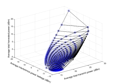
(a) System objective trade-off region for Case I.

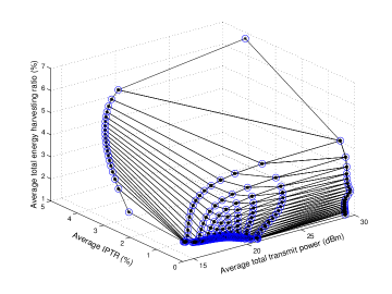
(b) System objective trade-off region for Case II.

Figure 3: Three-dimensional system objective trade-off regions achieved by the proposed optimal resource allocation scheme. Asterisk markers denote the trade-off region achieved by the resource allocation scheme and colored circles represent the Pareto frontier.

For the trade-off region for Case I in Figure 3(a), it can be observed that although the system design objectives of total transmit power minimization and total interference power leakage minimization do not share the same optimal solution (a single point which is the minimum of both objective functions), these two objectives are partially aligned with each other. Specifically, a large portion of the trade-off region is concentrated at the bottom of the figure. In other words, a resource allocation policy which minimizes the total transmit power can also reduce the total interference power leakage effectively and vice versa. On the contrary, the objective of total harvested power maximization conflicts with the other two objective functions. In particular, in order to maximize the total harvested power, the secondary transmitter has to transmit with full power in every time instant despite the imperfection of the CSI. The associated resource allocation policy with full power transmission corresponds to the top corner point in Figure 3(a). Besides, if the secondary transmitter employs a large transmit power, a high average total interference power leakage at the primary receivers will result. Furthermore, the total harvested power in the system is in the order of milliwatt which is sufficient to charge the sensor type idle secondary receivers, despite the existence of the primary receivers, cf. footnote 2.

For the trade-off region for Case II in Figure 3(b), it can be seen that a significant portion of the trade-off region is concentrated near the bottom and the remaining parts spread over the entire space of the figure. The fact that the trade-off region is condensed near the bottom indicates that resource allocation policies which minimize the total transmit power can also reduce the IPTR to a certain extent and vice versa. However, there also exist resource allocation policies that incur a high transmit power while achieving a low IPTR, i.e., the points located near an average total transmit power of $30$ dBm and average IPTR $=0.1\%$. This can be explained by the fact that the objective functions for energy harvesting efficiency maximization and IPTR minimization are invariant to a simultaneous positive scaling of both $\mathbf{W}$ and $\mathbf{V},$ e.g. $\frac{\mathrm{HP}(c\mathbf{W},c\mathbf{V})}{\mathrm{TP}(c\mathbf{W},c\mathbf{V})}=\frac{\mathrm{HP}(\mathbf{W},\mathbf{V})}{\mathrm{TP}(\mathbf{W},\mathbf{V})}$ and $\frac{\mathrm{IP}(c\mathbf{W},c\mathbf{V})}{\mathrm{TP}(c\mathbf{W},c\mathbf{V})}=\frac{\mathrm{IP}(\mathbf{W},\mathbf{V})}{\mathrm{TP}(\mathbf{W},\mathbf{V})}$ for $c>0$. As a result, if total transmit power minimization is not a system design objective in Problem $4$, i.e., $\lambda_{2}=0$, optimal solutions of Problem $4$ in the trade-off region may exist such that the secondary transmitter transmits with a high power while still satisfying all constraints. On the other hand, to achieve the maximum energy harvesting efficiency in the secondary network, i.e., the top corner point in Figure 3(b), the secondary transmitter has to transmit with maximum power which leads to a high average IPTR.

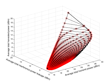
(a) System objective trade-off region for Case I.

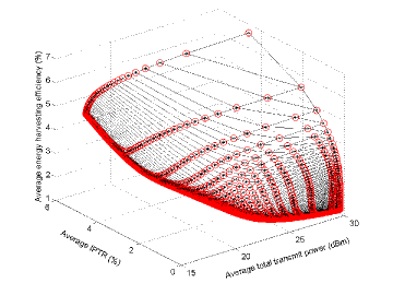
(b) System objectives trade-off region for Case II.

Figure 4: Three-dimensional system objective trade-off regions achieved by the baseline scheme. Asterisk markers denote the trade-off region achieved by the baseline resource allocation scheme and colored circles represent the Pareto frontier with respect to the baseline resource allocation scheme.

For comparison, in Figure 4, we plot the trade-off regions achieved by a baseline resource allocation scheme for Case I and Case II in Figure 3. For the baseline scheme, we adopt maximum ratio transmission (MRT) with respect to the desired secondary receiver for information beamforming matrix ${\mathbf{W}}$. In other words, the beamforming direction of matrix ${\mathbf{W}}$ is fixed and it has a rank-one structure. Then, we optimize the artificial noise covariance matrix $\mathbf{{V}}$ and the power of ${\mathbf{W}}$ in Problem $4$ via varying the values of $0\leq\lambda_{p}\leq 1,\forall p\in\{1,2,3\}$. We note that the proposed baseline scheme requires the same amount of CSI as the proposed optimal scheme. However, the baseline scheme does not fully exploit the available CSI for resource allocation optimization and, as a result, the required computational complexity is reduced roughly by half compared to the proposed optimal scheme.

As can be observed from Figures 3(a), 3(b), 4(a), and 4(b), the baseline scheme is effective in maximizing the energy harvesting efficiency and the total harvested power in the high transmit power regime and is able to approach the optimal trade-off region achieved by the proposed optimal SDP based resource allocation scheme. This can be explained by the fact that both the optimal scheme and the baseline scheme optimize the covariance matrix of the artificial noise which contributes most of the power transferred to the idle secondary receivers. In particular, by exploiting the spatial degrees of freedom offered by the multiple antennas, multiple narrow energy beams can be created via the proposed optimization framework for transfer of the artificial noise. The narrow energy beams help in focusing energy on the idle secondary receivers which increases the energy transfer efficiency. Nevertheless, when the total transmit power budget of the secondary transmitter is small, the baseline scheme may not be able to satisfy the QoS constraints which leads to a smaller trade-off region compared to the proposed optimal scheme.

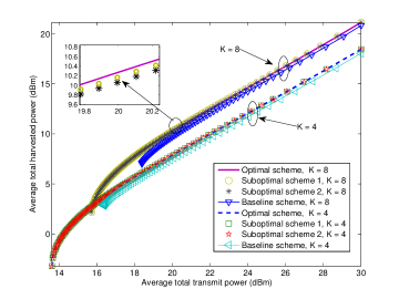
(a) Average total harvested power.

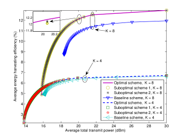
(b) Average energy harvesting efficiency.

Figure 5: Average total harvested power and average energy harvesting efficiency versus the average total transmit power of the secondary system for different resource allocation schemes and different numbers of secondary receivers, $K$.

V-B Average Total Harvested Power and Average Energy Harvesting Efficiency

Figures 5(a) and 5(b) depict the average total harvested power and the average energy harvesting efficiency of the secondary system versus the average total transmit power for different numbers of secondary receivers, $K$, respectively. The curves in Figures 5(a) and 5(b) are obtained for Case I and Case II, respectively. Specifically, for each case, we solve Problem 4 for $\lambda_{3}=0$ and $0\leq\lambda_{p}\leq 1,\forall p\in\{1,2\}$, where the values of $\lambda_{p},p\in\{1,2\},$ are uniformly varied for a step size of $0.01$ such that $\sum_{p}\lambda_{p}=1$. It can be observed from Figures 5(a) and 5(b) that the average total harvested power and the average energy harvesting efficiency are monotonically increasing functions with respect to the total transmit power. In other words, total harvested power/energy harvesting efficiency maximization and total transmit power minimization are conflicting system design objectives. Also, the proposed optimal scheme outperforms the baseline scheme. In particular, the proposed optimal scheme fully utilizes the available CSI and provides a larger trade-off region, e.g. $2.7$ dB less transmit power in the considered scenario compared to the baseline scheme in Figure 5(a). Besides, the two proposed suboptimal schemes perform close to the trade-off region achieved by the optimal SDP resource allocation scheme. Furthermore, all trade-off curves are shifted in the upper-right direction if the number of secondary receivers is increased. This is due to the fact that for a larger number of secondary users, there are more idle secondary receivers in the system harvesting the power radiated by the transmitter which improves the energy harvesting efficiency and the total harvested power. Also, having additional idle secondary receivers means that there are more potential eavesdroppers in the system. Thus, more artificial noise generation is required for neutralizing information leakage. We note that in all the considered scenarios, the proposed resource allocation schemes are able to guarantee the minimum secrecy data rate requirement of $C_{\mathrm{sec}}\geq 5.6582$ bit/s/Hz despite the imperfectness of the CSI.

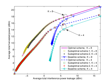
(a) Average total harvested power.

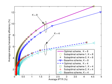
(b) Average energy harvesting efficiency.

Figure 6: Average total harvested power and average energy harvesting efficiency of the secondary system versus the average total interference power leakage and the average IPTR, respectively, for different resource allocation schemes and different numbers of secondary receivers, $K$.

Figures 6(a) and 6(b) show the average total harvested power and the average energy harvesting efficiency of the secondary system versus the average total interference power leakage and the average IPTR, respectively, for different numbers of desired secondary receivers, $K$. The curves in Figures 6(a) and 6(b) are obtained by solving Problem 4 for $\lambda_{2}=0$ and varying the values of $0\leq\lambda_{p}\leq 1,\forall p\in\{1,3\}$, uniformly for a step size of $0.01$ such that $\sum_{p}\lambda_{p}=1$ for Case I and Case II, respectively. The average total harvested power and the average energy harvesting efficiency increase with increasing average total interference power leakage and increasing average IPTR, respectively. This observation indicates that total harvested power maximization and energy harvesting efficiency maximization are conflicting with total interference power leakage minimization and IPTR minimization, respectively. Besides, the two proposed suboptimal schemes perform close to the trade-off curve achieved by the optimal resource allocation scheme. Furthermore, all the trade-off curves are shifted in the upper-right direction as the number of secondary receivers is increased. In fact, there are more potential eavesdroppers in the system when the number of idle secondary receivers increases. Thus, more artificial noise has to be radiated by the secondary transmitter for guaranteeing communication security which leads to a higher IPTR and a higher interference power leakage. On the other hand, the baseline scheme achieves a smaller trade-off region in both Figures 6(a) and 6(b) compared to the proposed optimal and suboptimal schemes. This performance gap reveals the importance of the optimization of beamforming matrix $\overline{\mathbf{W}}$ for minimizing the total interference power leakage and the IPTR.

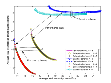
(a) Average total interference power leakage.

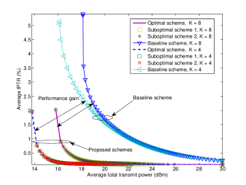
(b) Average IPTR.

Figure 7: Average total interference power leakage and average IPTR of the secondary system versus the average total transmit power for different resource allocation schemes and different numbers of secondary receivers, $K$. The double-sided arrows indicate the performance gain achieved by the proposed schemes compared to the baseline scheme.

V-C Average Total Interference Power Leakage and Average IPTR

Figures 7(a) and 7(b) depict the average total interference power leakage and the average IPTR of the secondary system versus the average total transmit power for different numbers of secondary receivers, $K$, respectively. The curves in Figures 7(a) and 7(b) are obtained by solving Problem 4 for Case I and Case II, respectively, by setting $\lambda_{1}=0$ and varying the values of $0\leq\lambda_{p}\leq 1,\forall p\in\{2,3\}$, uniformly for a step size of $0.01$ such that $\sum_{p}\lambda_{p}=1$. Interestingly, we observe from Figures 7(a) and 7(b) that a higher transmit power may not correspond to a stronger interference leakage to the primary system or a higher IPTR, if the degrees of freedom offered by the multiple antennas are properly exploited. Furthermore, the baseline scheme achieves a significantly worse trade-off compared to the proposed optimal and suboptimal schemes, e.g. $10$ dB more interference leakage in Figure 7(a). Also, a resource allocation policy that minimizes the total transmit power can only minimize the total interference power leakage simultaneously to a certain extent or vice versa in general. For minimizing the total interference power leakage, the secondary transmitter sacrifices some degrees of freedom to reduce the received strengths of both information signal and artificial noise at the primary receivers. Thus, fewer degrees of freedom are available for providing reliable and secure communication to the secondary receivers such that a higher transmit power is required. In fact, in the proposed optimal scheme, both the beamforming matrix $\mathbf{\overline{W}}$ and the artificial noise covariance matrix $\mathbf{\overline{V}}$ are jointly optimized for performing resource allocation based on the CSI of all receivers. In contrast, in the baseline scheme, the direction of the beamforming matrix is fixed which leads to fewer degrees of freedom for resource allocation. Thus, the baseline scheme performs worse than the proposed schemes. On the other hand, for a given required average interference leakage power or average IPTR, increasing the number of secondary receivers induces a higher transmit power in both cases. Indeed, constraint C2 on communication secrecy becomes more stringent for an increasing number of secondary receivers. In other words, it leads to a smaller feasible solution set for resource allocation optimization. As a result, the efficiency of the resource allocation schemes in jointly optimizing the multiple objective functions decreases for a larger number of secondary receivers $K$.

VI Conclusions

In this paper, we studied the resource allocation algorithm design for CR secondary networks with simultaneous wireless power transfer and secure communication based on a multi-objective optimization framework. We focused on three system design objectives: transmit power minimization, energy harvesting efficiency maximization, and IPTR minimization. Besides, the proposed multi-objective problem formulation includes total harvested power maximization and interference power leakage minimization as special cases. In addition, our problem formulation takes into account the imperfectness of the CSI of the idle secondary receivers and the primary receivers at the secondary transmitter. By utilizing the primal and dual optimal solutions of the SDP relaxed problem, the global optimal solution of the original problem can be constructed. Furthermore, two suboptimal resource allocation schemes were proposed for the case when the solution of the dual problem is unavailable. Simulation results illustrated the performance gains of the proposed schemes compared to a baseline scheme, and unveiled the trade-off between the considered system design objectives: (1) A resource allocation policy minimizing the total transmit power also leads to a low total interference power leakage in general; (2) energy harvesting efficiency maximization and transmit power minimization are conflicting system design objectives; (3) maximum energy harvesting efficiency is achieved at the expense of high interference power leakage and high transmit power.

Appendix

VI-A Proof of Proposition 1

The proof is based on the Charnes-Cooper transformation [27, 58]. By applying the change of variables in (23) to (III-E), Problem $1$ in (III-E) can be equivalently transformed to

$$\underset{\overline{\mathbf{W}},\overline{\mathbf{V}}\in\mathbb{H}^{N_{\mathrm{T}}},\xi}{\operatorname{\mathrm{minimize}}}\,\,\,\,\frac{-\sum_{k=1}^{K-1}\eta_{k}\operatorname{\mathrm{Tr}}(\mathbf{G}_{k}(\overline{\mathbf{W}}+\overline{\mathbf{V}}))}{\operatorname{\mathrm{Tr}}(\overline{\mathbf{W}})+\operatorname{\mathrm{Tr}}(\overline{\mathbf{V}})}$$ (42)

s.t. $$\mbox{$\overline{\mbox{C1}}$}-\mbox{$\overline{\mbox{C5}}$},\,\,\mbox{$\overline{\mbox{C6}}$:}\,\,\xi>0,\mbox{$\overline{\mbox{C7}}$:}\,\,\operatorname{\mathrm{Tr}}(\overline{\mathbf{W}})+\operatorname{\mathrm{Tr}}(\overline{\mathbf{V}})=1,\mbox{$\overline{\mbox{C8}}$}.$$

Now, we show that (42) is equivalent to

$$\underset{\overline{\mathbf{W}},\overline{\mathbf{V}}\in\mathbb{H}^{N_{\mathrm{T}}},\xi}{\operatorname{\mathrm{minimize}}}\,\,\,\,-\sum_{k=1}^{K-1}\eta_{k}\operatorname{\mathrm{Tr}}(\mathbf{G}_{k}(\overline{\mathbf{W}}+\overline{\mathbf{V}}))$$ (43)

s.t. $$\mbox{$\overline{\mbox{C1}}$}-\mbox{$\overline{\mbox{C5}}$},\,\,\mbox{$\overline{\mbox{C6}}$:}\,\,\xi\geq 0,\,\,\mbox{$\overline{\mbox{C7}}$:}\,\,\operatorname{\mathrm{Tr}}(\overline{\mathbf{W}})+\operatorname{\mathrm{Tr}}(\overline{\mathbf{V}})=1,\mbox{ $\overline{\mbox{C8}}$}.$$

We denote the optimal solution of (43) as $(\overline{\mathbf{W}}^{*},\overline{\mathbf{V}}^{*},\xi^{*})$. If $\xi^{*}=0$, then $\overline{\mathbf{W}}=\overline{\mathbf{V}}=\mathbf{0}$ according to $\overline{\mbox{C3}}$. Yet, this solution cannot satisfy $\overline{\mbox{C1}}$ for $\Gamma_{\mathrm{req}}>0$. As a result, without loss of generality and optimality, constraint $\xi>0$ can be replaced by $\xi\geq 0$. The equivalence between transformed Problems 2, 3, and 4 and their original problem formulations can be proved by following a similar approach as above.

VI-B Proof of Theorem 1

The proof is divided into two parts. In the first part, we investigate the structure of the optimal solution $\mathbf{\overline{W}}^{*}$ of the relaxed version of problem (IV-A). Then, in the second part, we propose a method to construct a solution $\mathbf{\widetilde{\Lambda}}\triangleq\{\mathbf{\widetilde{I}}^{\mathrm{PU}},\mathbf{\widetilde{E}}^{\mathrm{SU}},\widetilde{\xi},\widetilde{\tau},\boldsymbol{\widetilde{\gamma}},\boldsymbol{\widetilde{\delta}},\boldsymbol{\widetilde{\varphi}},\boldsymbol{\widetilde{\omega}},{\mathbf{\widetilde{V}}},\mathbf{{\widetilde{W}}}\}$ that achieves the same objective value as $\mathbf{\Lambda}^{*}\triangleq\{\mathbf{I}^{\mathrm{PU}*},\mathbf{E}^{\mathrm{SU}*},\xi^{*},\tau^{*},$ $\boldsymbol{\gamma^{*}},\boldsymbol{\delta^{*}},\boldsymbol{\varphi^{*}},\boldsymbol{\omega^{*}},\overline{\mathbf{V}}^{*},\mathbf{\overline{W}}^{*}\}$ but admits a rank-one $\mathbf{\widetilde{W}}$.

It can be shown that the relaxed version of problem (IV-A) is jointly convex with respect to the optimization variables and satisfies Slater’s constraint qualification. As a result, the Karush-Kuhn-Tucker (KKT) conditions are necessary and sufficient conditions [44] for the optimal solution of the relaxed version of problem (IV-A). The Lagrangian function of the relaxed version of problem (IV-A) is given by

$${\cal L} = \operatorname{\mathrm{Tr}}\Big{(}\big{(}\mathbf{I}_{N_{\mathrm{T}}}(\alpha+\mu)-\mathbf{Y}-\beta\mathbf{H}\big{)}\overline{\mathbf{W}}\Big{)}$$ (44)

$$- \sum_{k=1}^{K-1}\operatorname{\mathrm{Tr}}\Big{(}\mathbf{S}_{\mathrm{\overline{C2}}_{k}}\big{(}\overline{\mathbf{W}},\overline{\mathbf{V}},\delta_{k}\big{)}\mathbf{D}_{\mathrm{\overline{C2}}_{k}}\Big{)}$$

$$- \sum_{j=1}^{J}\operatorname{\mathrm{Tr}}\Big{(}\mathbf{S}_{\mathrm{\overline{C3}}_{j}}\big{(}\overline{\mathbf{W}},\overline{\mathbf{V}},\xi,\gamma_{j}\big{)}\mathbf{D}_{\mathrm{\overline{C3}}_{j}}\Big{)}$$

$$- \sum_{j=1}^{J}\operatorname{\mathrm{Tr}}\Big{(}\mathbf{S}_{\mathrm{\overline{C11}}_{j}}\big{(}\overline{\mathbf{W}},\overline{\mathbf{V}},\xi,\omega_{j}\big{)}\mathbf{D}_{\mathrm{\overline{C11}}_{j}}\Big{)}$$

$$- \sum_{k=1}^{K-1}\operatorname{\mathrm{Tr}}\Big{(}\mathbf{S}_{\mathrm{\overline{C10}}_{k}}\big{(}\overline{\mathbf{W}},\overline{\mathbf{V}},\xi,\varphi_{k}\big{)}\mathbf{D}_{\mathrm{\overline{C10}}_{k}}\Big{)}+\Omega,$$

where $\Omega$ denotes the collection of the terms that only involve variables that are not relevant for the proof. $\beta,\alpha\geq 0$, and $\mu$ are the Lagrange multipliers associated with constraints $\overline{\mbox{C1}}$, $\overline{\mbox{C4}}$, and $\overline{\mbox{C7}}$, respectively. Matrix $\mathbf{Y}\succeq\mathbf{0}$ is the Lagrange multiplier matrix for the semidefinite constraint on matrix $\overline{\mathbf{W}}$ in $\overline{\mbox{C4}}$. $\mathbf{D}_{\mathrm{\overline{C2}}_{k}}\succeq\mathbf{0},\forall k\in\{1,\,\ldots,\,K-1\},$ and $\mathbf{D}_{\mathrm{\overline{C3}}_{j}}\succeq\mathbf{0},\forall j\in\{1,\,\ldots,\,J\}$, are the Lagrange multiplier matrices for the maximum tolerable SINRs of the idle secondary receivers and the primary receivers in $\overline{\mbox{C2}}$ and $\overline{\mbox{C3}}$, respectively. $\mathbf{D}_{\mathrm{\overline{C10}}_{k}}\succeq\mathbf{0},\forall k\in\{1,\,\ldots,\,K-1\},$ and $\mathbf{D}_{\mathrm{\overline{C11}}_{j}}\succeq\mathbf{0},\forall j\in\{1,\,\ldots,\,J\}$, are the Lagrange multiplier matrices associated with constraints $\overline{\mbox{C10}}$ and $\overline{\mbox{C11}}$, respectively. In the following, we focus on the KKT conditions related to the optimal $\mathbf{\overline{W}}^{*}$:

$$\mathbf{Y}^{*},\mathbf{D}^{*}_{\mathrm{\overline{C2}}_{k}},\mathbf{D}^{*}_{\mathrm{\overline{C3}}_{j}},\mathbf{D}^{*}_{\mathrm{\overline{C10}}_{k}},\mathbf{D}^{*}_{\mathrm{\overline{C11}}_{j}} \succeq \mathbf{0},\alpha^{*},\beta^{*}\geq 0,\mu^{*},$$ (45)

$$\mathbf{Y^{*}\overline{\mathbf{W}}^{*}} = \mathbf{0},$$ (46)

$$\nabla_{\overline{\mathbf{W}}^{*}}{\cal L} = \mathbf{0},$$ (47)

where $\mathbf{Y}^{*},\mathbf{D}^{*}_{\mathrm{\overline{C2}}_{k}},\mathbf{D}^{*}_{\mathrm{\overline{C3}}_{j}},\mathbf{D}^{*}_{\mathrm{\overline{C10}}_{k}},\mathbf{D}^{*}_{\mathrm{\overline{C11}}_{j}},\mu^{*},\beta^{*}$, and $\alpha^{*}$ are the optimal Lagrange multipliers for the dual problem of (IV-A). From the complementary slackness condition in (46), we observe that the columns of $\overline{\mathbf{W}}^{*}$ are required to lie in the null space of $\mathbf{Y}^{*}$ for $\overline{\mathbf{W}}^{*}\neq\mathbf{0}$. Thus, we study the composition of $\mathbf{Y}^{*}$ to obtain the structure of $\overline{\mathbf{W}}^{*}$. The KKT condition in (47) can be expressed as

$$\mathbf{Y}^{*}+\beta^{*}\mathbf{H}$$ (48)

$$= \mathbf{I}_{N_{\mathrm{T}}}(\mu^{*}+\alpha^{*})+\sum_{k=1}^{K-1}\mathbf{U}_{\mathbf{g}_{k}}\Big{(}\frac{\mathbf{D}^{*}_{\mathrm{\overline{C2}}_{k}}}{\Gamma_{\mathrm{tol}_{k}}}-\mathbf{D}_{\mathrm{\overline{C10}}_{k}}^{*}\Big{)}\mathbf{U}_{\mathbf{g}_{k}}^{H}$$

$$+ \sum_{j=1}^{J}\mathbf{U}_{\mathbf{l}_{j}}\Big{(}\frac{\mathbf{D}^{*}_{\mathrm{\overline{C3}}_{j}}}{\Gamma_{\mathrm{tol}_{j}}^{\mathrm{PU}}}+\mathbf{D}_{\mathrm{\overline{C11}}_{j}}^{*}\Big{)}\mathbf{U}_{\mathbf{l}_{j}}^{H}.$$

For notational simplicity, we define

$$\mathbf{A}^{*} = \mathbf{I}_{N_{\mathrm{T}}}(\mu^{*}+\alpha^{*})+\sum_{k=1}^{K-1}\mathbf{U}_{\mathbf{g}_{k}}\Big{(}\frac{\mathbf{D}^{*}_{\mathrm{\overline{C2}}_{k}}}{\Gamma_{\mathrm{tol}_{k}}}-\mathbf{D}_{\mathrm{\overline{C10}}_{k}}^{*}\Big{)}\mathbf{U}_{\mathbf{g}_{k}}^{H}$$ (49)

$$+ \sum_{j=1}^{J}\mathbf{U}_{\mathbf{l}_{j}}\Big{(}\frac{\mathbf{D}^{*}_{\mathrm{\overline{C3}}_{j}}}{\Gamma_{\mathrm{tol}_{j}}^{\mathrm{PU}}}+\mathbf{D}_{\mathrm{\overline{C11}}_{j}}^{*}\Big{)}\mathbf{U}_{\mathbf{l}_{j}}^{H}.$$

Besides, there exists at least one optimal solution with $\beta^{*}>0$, i.e., constraint $\overline{\mbox{C1}}$ is satisfied with equality. Suppose that for the optimal solution, constraint $\overline{\mbox{C1}}$ is satisfied with strict inequality, i.e., $\frac{\operatorname{\mathrm{Tr}}(\mathbf{H}\overline{\mathbf{W}}^{*})}{\operatorname{\mathrm{Tr}}(\mathbf{H}\overline{\mathbf{V}}^{*})+\sigma_{\mathrm{z}}^{2}\xi^{*}}>\Gamma_{\mathrm{req}}$. Then, we can replace $\xi^{*}$ with $\overline{\xi}^{*}=\xi^{*}c$ for $c>1$ such that $\overline{\mbox{C1}}$ is satisfied with equality. We note that the new solution $\overline{\xi}^{*}$ not only satisfies all the constraints, but also provides a larger feasible solution set for minimizing $\tau$, cf. constraints $\overline{\mbox{C4}}$ and $\overline{\mbox{C9}}$b. As a result, there always exist at least one optimal solution such that constraint $\overline{\mbox{C1}}$ is satisfied with equality. In order to obtain the optimal solution in practice, we can replace the inequality “$\geq$”with equality “$=$” in $\overline{\mbox{C2}}$ without loss of optimality. From (48) and (49), we can express the Lagrange multiplier matrix $\mathbf{Y}^{*}$ as

$$\mathbf{Y}^{*}=\mathbf{A}^{*}-\beta^{*}\mathbf{H},$$ (50)

where $\beta^{*}\mathbf{H}$ is a rank-one matrix since $\beta^{*}>0$. Without loss of generality, we define $r=\operatorname{\mathrm{Rank}}(\mathbf{A}^{*})$ and the orthonormal basis of the null space of $\mathbf{A}^{*}$ as $\mathbf{\mathbf{\Upsilon}}\in\mathbb{C}^{N_{\mathrm{T}}\times(N_{\mathrm{T}}-r)}$ such that $\mathbf{A}^{*}\mathbf{\Upsilon}=\mathbf{0}$ and $\operatorname{\mathrm{Rank}}(\mathbf{\Upsilon})=N_{\mathrm{T}}-r$. Let ${\boldsymbol{\phi}}_{t}\in\mathbb{C}^{N_{\mathrm{T}}\times 1}$, $1\leq t\leq N_{\mathrm{T}}-r$, denote the $t$-th column of $\mathbf{\Upsilon}$. By exploiting [30, Proposition 4.1], it can be shown that $\mathbf{H}\mathbf{\Upsilon}=\mathbf{0}$ and we can express the optimal solution of $\overline{\mathbf{W}}^{*}$ as

$$\overline{\mathbf{W}}^{*}=\sum_{t=1}^{N_{\mathrm{T}}-r}\psi_{t}{\boldsymbol{\phi}}_{t}{\boldsymbol{\phi}}_{t}^{H}+\underbrace{f\mathbf{u}\mathbf{u}^{H}}_{\mbox{Rank-one}},$$ (51)

where $\psi_{t}\geq 0,\forall t\in\{1,\ldots,N_{\mathrm{T}}-r\},$ and $f>0$ are positive scalars and $\mathbf{u}\in\mathbb{C}^{N_{\mathrm{T}}\times 1}$, $\lVert\mathbf{u}\rVert=1$, satisfies $\mathbf{u}^{H}\mathbf{\Upsilon}=\mathbf{0}$.

In the second part of the proof, for $\operatorname{\mathrm{Rank}}(\overline{\mathbf{W}}^{*})>1$, we construct another solution $\mathbf{\widetilde{\Lambda}}\triangleq\{\mathbf{\widetilde{I}}^{\mathrm{PU}},\mathbf{\widetilde{E}}^{\mathrm{SU}},\widetilde{\xi},\widetilde{\tau},$ $\boldsymbol{\widetilde{\gamma},\widetilde{\delta},\widetilde{\varphi},\widetilde{\omega}},{\mathbf{\widetilde{V}}},\mathbf{{\widetilde{W}}}\}$ based on (51). Let

$$\mathbf{\widetilde{W}} = f\mathbf{u}\mathbf{u}^{H}=\overline{\mathbf{W}}^{*}-\sum_{t=1}^{N_{\mathrm{T}}-r}\psi_{t}{\boldsymbol{\phi}}_{t}{\boldsymbol{\phi}}_{t}^{H},$$ (52)

$$\mathbf{\widetilde{V}} = \overline{\mathbf{V}}^{*}+\sum_{t=1}^{N_{\mathrm{T}}-r}\psi_{t}{\boldsymbol{\phi}}_{t}{\boldsymbol{\phi}}_{t}^{H},$$ (53)

$$\mathbf{\widetilde{I}}^{\mathrm{PU}} = \mathbf{I}^{\mathrm{PU}*},\,\,\mathbf{\widetilde{E}}^{\mathrm{SU}}=\mathbf{E}^{\mathrm{SU}*},\,\,\widetilde{\xi}=\xi^{*},\,\,$$ (54)

$$\widetilde{\tau} = \tau^{*},\,\,\boldsymbol{\widetilde{\gamma}}=\boldsymbol{\gamma}^{*},\,\,\boldsymbol{\widetilde{\delta}}=\boldsymbol{\delta}^{*},\,\,\boldsymbol{\widetilde{\varphi}}=\boldsymbol{\widetilde{\varphi}}^{*},\,\,\boldsymbol{\widetilde{\omega}}=\boldsymbol{\omega}^{*}.$$ (55)

Then, we substitute the constructed solution $\mathbf{\widetilde{\Lambda}}$ into the objective function and the constraints in (IV-A) which yields the equations in (56) on the top of next page.

$$\mbox{Objective value:}\quad\widetilde{\tau}=\tau^{*}$$ (56)

$$\overline{\mbox{C1}} \frac{\operatorname{\mathrm{Tr}}(\mathbf{\mathbf{H}\widetilde{W}})}{\operatorname{\mathrm{Tr}}(\mathbf{H}\mathbf{\widetilde{V}})+\widetilde{\xi}\sigma_{\mathrm{z}}^{2}}=\frac{\operatorname{\mathrm{Tr}}\big{(}\mathbf{H}(\overline{\mathbf{W}}^{*}-\sum_{t=1}^{N_{\mathrm{T}}-r}\psi_{t}{\boldsymbol{\phi}}_{t}{\boldsymbol{\phi}}_{t}^{H})\big{)}}{\operatorname{\mathrm{Tr}}(\mathbf{H}(\overline{\mathbf{V}}^{*}+\sum_{t=1}^{N_{\mathrm{T}}-r}\psi_{t}{\boldsymbol{\phi}}_{t}{\boldsymbol{\phi}}_{t}^{H}))+\xi^{*}\sigma_{\mathrm{z}}^{2}}=\frac{\operatorname{\mathrm{Tr}}(\overline{\mathbf{W}}^{*}\mathbf{H})}{\operatorname{\mathrm{Tr}}(\mathbf{H}\overline{\mathbf{V}}^{*})+\xi^{*}\sigma_{\mathrm{z}}^{2}}\geq\Gamma_{\mathrm{req}},$$:

$$\overline{\mbox{C2}} \mathbf{S}_{\mathrm{\overline{C2}}_{k}}(\mathbf{\widetilde{W}},\mathbf{\widetilde{V}},\widetilde{\xi},\widetilde{\delta}_{k})\succeq\mathbf{S}_{\mathrm{\overline{C2}}_{k}}(\overline{\mathbf{W}}^{*},\overline{\mathbf{V}}^{*},\xi^{*},\delta_{k}^{*})$$:

$$+ \mathbf{U}_{\mathbf{g}_{k}}^{H}\Big{[}\sum_{t=1}^{N_{\mathrm{T}}-r}\psi_{t}{\boldsymbol{\phi}}_{t}{\boldsymbol{\phi}}_{t}^{H}\Big{]}\mathbf{U}_{\mathbf{g}_{k}}\Big{(}1+\frac{1}{\Gamma_{\mathrm{tol}_{k}}}\Big{)}\succeq\mathbf{0},\forall k\in\{1,\ldots,K-1\},$$

$$\overline{\mbox{C3}} \mathbf{S}_{\mathrm{\overline{C3}}_{j}}(\mathbf{\widetilde{W}},\mathbf{\widetilde{V}},\widetilde{\xi},\widetilde{\gamma}_{j})\succeq\mathbf{S}_{\mathrm{\overline{C3}}_{j}}(\overline{\mathbf{W}}^{*},\overline{\mathbf{V}}^{*},\xi^{*},\gamma_{j}^{*})$$:

$$+ \mathbf{U}_{\mathbf{l}_{j}}^{H}\Big{[}\sum_{t=1}^{N_{\mathrm{T}}-r}\psi_{t}{\boldsymbol{\phi}}_{t}{\boldsymbol{\phi}}_{t}^{H}\Big{]}\mathbf{U}_{\mathbf{l}_{j}}\Big{(}1+\frac{1}{\Gamma_{\mathrm{tol}_{j}}^{\mathrm{PU}}}\Big{)}\succeq\mathbf{0},\forall j\in\{1,\ldots,J\},$$

$$\overline{\mbox{C4}} \operatorname{\mathrm{Tr}}({\mathbf{\widetilde{W}}})+\operatorname{\mathrm{Tr}}({\mathbf{\widetilde{V}}})=\operatorname{\mathrm{Tr}}(\overline{\mathbf{W}}^{*})+\operatorname{\mathrm{Tr}}(\overline{\mathbf{V}}^{*})\leq P_{\max}\widetilde{\xi},$$:

$$\overline{\mbox{C5}} \mathbf{\widetilde{W}},\mathbf{\widetilde{V}}\succeq\mathbf{0},\quad\mbox{$\overline{\mbox{C6}}$:}\,\,\widetilde{\xi}\geq 0,\quad\mbox{$\overline{\mbox{C7}}$:}\operatorname{\mathrm{Tr}}({\mathbf{\widetilde{W}}})+\operatorname{\mathrm{Tr}}({\mathbf{\widetilde{V}}})=\operatorname{\mathrm{Tr}}(\overline{\mathbf{W}}^{*})+\operatorname{\mathrm{Tr}}(\overline{\mathbf{V}}^{*})=1,$$:

$$\overline{\mbox{C9}} \frac{\lambda_{1}}{\lvert F_{1}^{*}\rvert}\Big{(}\sum_{k=1}^{K-1}\widetilde{E}_{k}^{\mathrm{SU}}-F_{1}^{*}\Big{)}\leq\widetilde{\tau},\,\,\mbox{$\overline{\mbox{C9}}$b: }\frac{\lambda_{2}}{\lvert F_{2}^{*}\rvert}\Big{(}\frac{1}{\widetilde{\xi}}-F_{2}^{*}\Big{)}\leq\widetilde{\tau},\,\,\mbox{$\overline{\mbox{C9}}$c: }\frac{\lambda_{3}}{\lvert F_{3}^{*}\rvert}\Big{(}\sum_{j=1}^{J}\widetilde{I}_{j}^{\mathrm{PU}}-F_{3}^{*}\Big{)}\leq\widetilde{\tau},$$a:

$$\overline{\mbox{C10}} \mathbf{S}_{\mathrm{\overline{C10}}_{k}}({\mathbf{\widetilde{W}}},{\mathbf{\widetilde{V}}},\widetilde{E}_{k}^{\mathrm{SU}},\widetilde{\varphi}_{k})=\mathbf{S}_{\mathrm{\overline{C10}}_{k}}(\overline{\mathbf{W}}^{*},\overline{\mathbf{V}}^{*},E_{k}^{\mathrm{SU}*},\varphi_{k}^{*})\succeq\mathbf{0},\forall k,$$:

$$\overline{\mbox{C11}} \mathbf{S}_{\mathrm{\overline{C11}}_{j}}({\mathbf{\widetilde{W}}},{\mathbf{\widetilde{V}}},\widetilde{I}_{j}^{\mathrm{PU}},\widetilde{\omega}_{j})=\mathbf{S}_{\mathrm{\overline{C11}}_{j}}(\overline{\mathbf{W}}^{*},\overline{\mathbf{V}}^{*},I_{j}^{\mathrm{PU}*},\omega_{j}^{*})\succeq\mathbf{0},\forall j,$$:

$$\mbox{$\overline{\mbox{C12}}$: }\widetilde{\delta}_{k}\geq 0,\forall k,\,\,\,\,\mbox{$\overline{\mbox{C13}}$: }\widetilde{\gamma}_{j}\geq 0,\forall j,\,\,\,\,\mbox{$\overline{\mbox{C14}}$: }\widetilde{\varphi}_{k}\geq 0,\forall k,\,\,\,\,\mbox{$\overline{\mbox{C15}}$: }\widetilde{\omega}_{j}\geq 0,\forall j.$$

It can be seen from (56) that the constructed solution set $\mathbf{\widetilde{\Lambda}}$ achieves the same optimal value as the optimal solution $\mathbf{\Lambda}^{*}$ while satisfying all the constraints. Thus, $\mathbf{\widetilde{\Lambda}}$ is also an optimal solution of (IV-A). Besides, the constructed beamforming matrix $\mathbf{\widetilde{W}}$ is a rank-one matrix, i.e., $\operatorname{\mathrm{Rank}}(\mathbf{\widetilde{W}})=1$. On the other hand, we can obtain the values of $f$ and $\psi_{t}$ in (52) by substituting the variables in (52) into the relaxed version of (IV-A) and solving the resulting convex optimization problem for $f$ and $\psi_{t}$.

References

- [1] D. W. K. Ng, L. Xiang, and R. Schober, “Multi-Objective Beamforming for Secure Communication in Systems with Wireless Information and Power Transfer,” in Proc. IEEE Personal, Indoor and Mobile Radio Commun. Sympos., Sep. 2013, pp. 7 – 12.
- [2] “Facilitating Opportunities for Flexible, Efficient, and Reliable Spectrum Use Employing Cognitive Radio Technologies,” Federal Communications Commission, Tech. Rep., 2002, FCC 02-155.
- [3] Y.-C. Liang, K.-C. Chen, G. Li, and P. Mahonen, “Cognitive Radio Networking and Communications: An Overview,” IEEE Trans. Veh. Technol., vol. 60, pp. 3386–3407, Sep. 2011.
- [4] X. Chen, H.-H. Chen, and W. Meng, “Cooperative Communications for Cognitive Radio Networks – 2014; From Theory to Applications,” IEEE Commun. Surveys Tuts., vol. 16, pp. 1180–1192, Mar. 2014.
- [5] O. Akan, O. Karli, and O. Ergul, “Cognitive Radio Sensor Networks,” IEEE Netw., vol. 23, pp. 34–40, Jul. 2009.
- [6] X. Lu, P. Wang, D. Niyato, and E. Hossain, “Dynamic Spectrum Access in Cognitive Radio Networks with RF Energy Harvesting,” IEEE Wireless Commun., vol. 21, pp. 102–110, Jun. 2014.
- [7] G. Ganesan and Y. Li, “Cooperative Spectrum Sensing in Cognitive Radio, Part I: Two User Networks,” IEEE Trans. Wireless Commun., vol. 6, pp. 2204–2213, Jun. 2007.
- [8] Y.-C. Liang, Y. Zeng, E. Peh, and A. T. Hoang, “Sensing-Throughput Tradeoff for Cognitive Radio Networks,” IEEE Trans. Wireless Commun., vol. 7, pp. 1326–1337, Apr. 2008.
- [9] H. Islam, Y.-C. Liang, and A. T. Hoang, “Joint Beamforming and Power Control in the Downlink of Cognitive Radio Networks,” in Proc. IEEE Wireless Commun. and Networking Conf., Apr. 2007, pp. 21–26.
- [10] L. Zhang, Y.-C. Liang, Y. Xin, and H. Poor, “Robust Cognitive Beamforming with Partial Channel State Information,” IEEE Trans. Wireless Commun., vol. 8, pp. 4143–4153, Aug. 2009.
- [11] G. Zheng, K.-K. Wong, and B. Ottersten, “Robust Cognitive Beamforming With Bounded Channel Uncertainties,” IEEE Trans. Signal Process., vol. 57, pp. 4871–4881, Dec. 2009.
- [12] P. Yeoh, M. Elkashlan, N. Yang, D. da Costa, and T. Duong, “Unified Analysis of Transmit Antenna Selection in MIMO Multirelay Networks,” IEEE Trans. Veh. Technol., vol. 62, pp. 933–939, Feb 2013.
- [13] P. L. Yeoh, M. Elkashlan, T. Duong, N. Yang, and D. da Costa, “Transmit Antenna Selection for Interference Management in Cognitive Relay Networks,” IEEE Trans. Veh. Technol., vol. 63, pp. 3250–3262, Sep. 2014.
- [14] Powercast Coporation, “RF Energy Harvesting and Wireless Power for Low-Power Applications, year = 2011, url = http://www.mouser.com/pdfdocs/Powercast-Overview-2011-01-25.pdf,.”
- [15] J. Yang and S. Ulukus, “Optimal Packet Scheduling in an Energy Harvesting Communication System,” IEEE Trans. Commun., vol. 60, pp. 220–230, Jan. 2012.
- [16] I. Krikidis, S. Timotheou, S. Nikolaou, G. Zheng, D. W. K. Ng, and R. Schober, “Simultaneous Wireless Information and Power Transfer in Modern Communication Systems,” IEEE Commun. Mag., vol. 52, no. 11, pp. 104–110, Nov. 2014.
- [17] Z. Ding, C. Zhong, D. W. K. Ng, M. Peng, H. A. Suraweera, R. Schober, and H. V. Poor, “Application of Smart Antenna Technologies in Simultaneous Wireless Information and Power Transfer,” IEEE Commun. Magazine, vol. 53, no. 4, pp. 86–93, Apr. 2015.
- [18] X. Chen, Z. Zhang, H.-H. Chen, and H. Zhang, “Enhancing Wireless Information and Power Transfer by Exploiting Multi-Antenna Techniques,” IEEE Commun. Magazine, no. 4, pp. 133–141, Apr. 2015.
- [19] L. Varshney, “Transporting Information and Energy Simultaneously,” in Proc. IEEE Intern. Sympos. on Inf. Theory, Jul. 2008, pp. 1612 –1616.
- [20] P. Grover and A. Sahai, “Shannon Meets Tesla: Wireless Information and Power Transfer,” in Proc. IEEE Intern. Sympos. on Inf. Theory, Jun. 2010, pp. 2363 –2367.
- [21] J. Park and B. Clerckx, “Joint Wireless Information and Energy Transfer in a Two-User MIMO Interference Channel,” IEEE Trans. Wireless Commun., vol. 12, pp. 4210–4221, Aug. 2013.
- [22] X. Zhou, R. Zhang, and C. Ho, “Wireless Information and Power Transfer: Architecture Design and Rate-Energy Tradeoff,” IEEE Trans. Commun., vol. 61, pp. 4754 – 4767, Nov. 2013.
- [23] K. Huang and E. Larsson, “Simultaneous Information and Power Transfer for Broadband Wireless Systems,” IEEE Trans. Signal Process., vol. 61, pp. 5972–5986, Dec. 2013.
- [24] D. W. K. Ng, E. S. Lo, and R. Schober, “Wireless Information and Power Transfer: Energy Efficiency Optimization in OFDMA Systems,” IEEE Trans. Wireless Commun., vol. 12, pp. 6352 – 6370, Dec. 2013.
- [25] X. Chen and L. Lei, “Energy-Efficient Optimization for Physical Layer Security in Multi-Antenna Downlink Networks with QoS Guarantee,” IEEE Commun. Lett., vol. 17, pp. 637–640, Apr. 2013.
- [26] D. W. K. Ng, E. S. Lo, and R. Schober, “Energy-Efficient Resource Allocation for Secure OFDMA Systems,” IEEE Trans. Veh. Technol., vol. 6, pp. 2572–2585, Jul. 2012.
- [27] W.-C. Liao, T.-H. Chang, W.-K. Ma, and C.-Y. Chi, “QoS-Based Transmit Beamforming in the Presence of Eavesdroppers: An Optimized Artificial-Noise-Aided Approach,” IEEE Trans. Signal Process., vol. 59, pp. 1202–1216, Mar. 2011.
- [28] Y. Pei, Y.-C. Liang, L. Zhang, K. Teh, and K. H. Li, “Secure Communication Over MISO Cognitive Radio Channels,” IEEE Trans. Wireless Commun., vol. 9, pp. 1494–1502, Apr. 2010.
- [29] D. W. K. Ng, E. S. Lo, and R. Schober, “Robust Beamforming for Secure Communication in Systems with Wireless Information and Power Transfer,” IEEE Trans. Wireless Commun., vol. 13, pp. 4599–4615, Aug. 2014.
- [30] L. Liu, R. Zhang, and K.-C. Chua, “Secrecy Wireless Information and Power Transfer with MISO Beamforming,” IEEE Trans. Signal Process., vol. 62, pp. 1850–1863, Apr. 2014.
- [31] D. W. K. Ng and R. Schober, “Secure and Green SWIPT in Distributed Antenna Networks with Limited Backhaul Capacity,” submitted to IEEE Trans. Wireless Commun., 2014. [Online]. Available: http://arxiv.org/abs/1410.3065
- [32] S. Leng, D. W. K. Ng, and R. Schober, “Power Efficient and Secure Multiuser Communication Systems with Wireless Information and Power Transfer,” in Proc. IEEE Intern. Commun. Conf., Jun. 2014.
- [33] X. Chen, J. Chen, and T. Liu, “Secure Wireless Information and Power Transfer in Large-Scale MIMO Relaying Systems with Imperfect CSI,” in Proc. IEEE Global Telecommun. Conf., Dec. 2014, pp. 4131–4136.
- [34] M. Elkashlan, L. Wang, T. Duong, G. Karagiannidis, and A. Nallanathan, “On the Security of Cognitive Radio Networks,” IEEE Trans. Veh. Technol., vol. PP, no. 99, 2014.
- [35] Texas Instruments Incorporated. (2012) Msp430f2274. [Online]. Available: http://www.ti.com/product/msp430f2274
- [36] K. Hamdi, W. Zhang, and K. Letaief, “Joint Beamforming and Scheduling in Cognitive Radio Networks,” in Proc. IEEE Global Telecommun. Conf., Nov. 2007, pp. 2977–2981.
- [37] A. D. Wyner, “The Wire-Tap Channel,” Tech. Rep., Oct 1975.
- [38] F. Philipp, P. Zhao, F. Samman, M. Glesner, K. Dassanayake, S. Maheswararajah, and S. Halgamuge, “Adaptive Wireless Sensor Networks Powered by Hybrid Energy Harvesting for Environmental Monitoring,” in IEEE Intern. Conf. on Inf. and Autom. for Sustainability, Sep. 2012, pp. 285 –289.
- [39] Y. Tan and S. Panda, “Energy Harvesting From Hybrid Indoor Ambient Light and Thermal Energy Sources for Enhanced Performance of Wireless Sensor Nodes,” IEEE Trans. on Ind. Electron., vol. 58, pp. 4424–4435, Sep. 2011.
- [40] G. Zheng, K. K. Wong, and T. S. Ng, “Robust Linear MIMO in the Downlink: A Worst-Case Optimization with Ellipsoidal Uncertainty Regions,” EURASIP J. Adv. Signal Process., vol. 2008, 2008, Article ID 609028.
- [41] C. Shen, T.-H. Chang, K.-Y. Wang, Z. Qiu, and C.-Y. Chi, “Distributed Robust Multicell Coordinated Beamforming With Imperfect CSI: An ADMM Approach,” IEEE Trans. Signal Process., vol. 60, pp. 2988–3003, Jun. 2012.
- [42] N. Vucic and H. Boche, “Robust QoS-Constrained Optimization of Downlink Multiuser MISO Systems,” IEEE Trans. Signal Process., vol. 57, pp. 714–725, Feb. 2009.
- [43] J. Wang and D. Palomar, “Worst-Case Robust MIMO Transmission With Imperfect Channel Knowledge,” IEEE Trans. Signal Process., vol. 57, pp. 3086–3100, Aug. 2009.
- [44] S. Boyd and L. Vandenberghe, Convex Optimization. Cambridge University Press, 2004.
- [45] Q. Li and W.-K. Ma, “Optimal and Robust Transmit Designs for MISO Channel Secrecy by Semidefinite Programming,” IEEE Trans. Signal Process., vol. 59, pp. 3799–3812, Aug. 2011.
- [46] I. Wajid, M. Pesavento, Y. Eldar, and D. Ciochina, “Robust Downlink Beamforming With Partial Channel State Information for Conventional and Cognitive Radio Networks,” IEEE Trans. Signal Process., vol. 61, pp. 3656–3670, Jul. 2013.
- [47] R. T. Marler and J. S. Arora, “Survey of Multi-objective Optimization Methods for Engineering,” Structural and Multidisciplinary Optimization, vol. 26, pp. 369–395, Apr. 2004.
- [48] E. Björnson and E. Jorswieck, Optimal Resource Allocation in Coordinated Multi-Cell Systems. Now Publishers Inc., 2013.
- [49] M. Bengtsson and B. Ottersten, “Optimal Downlink Beamforming using Semidefinite Optimization,” in Proc. Annual Allerton Conf. on Commun., Control and Computing, Sep. 1999, pp. 987 –996.
- [50] Z.-Q. Luo, W.-K. Ma, A.-C. So, Y. Ye, and S. Zhang, “Semidefinite Relaxation of Quadratic Optimization Problems,” IEEE Trans. Signal Process., vol. 27, pp. 20–34, May 2010.
- [51] J. F. Sturm, “Using SeDuMi 1.02, A MATLAB Toolbox for Optimization over Symmetric Cones,” Optimiz. Methods and Software, vol. 11-12, pp. 625–653, Sep. 1999.
- [52] M. Grant and S. Boyd, “CVX: Matlab Software for Disciplined Convex Programming, version 2.0 beta,” http://cvxr.com/cvx, Sep. 2013.
- [53] T. H. Cormen, C. E. Leiserson, and R. L. R. amd Clifford Stein, Introduction to Algorithms, 3rd ed. The MIT Press, 2009.
- [54] B. Choi and G. Lee, “New Complexity Analysis for Primal-Dual Interior-Point Methods for Self-Scaled Optimization Problems,” Fixed Point Theory and Applications, no. 1, p. 213, Dec. 2012.
- [55] G. Wang and Y. Bai, “A New Primal-Dual Path-Following Interior-Point Algorithm for Semidefinite Optimization,” Journal of Mathematical Analysis and Applications, vol. 353, pp. 339 – 349, 2009.
- [56] N. Sidiropoulos, T. Davidson, and Z.-Q. Luo, “Transmit Beamforming for Physical-Layer Multicasting,” IEEE Trans. Signal Process., vol. 54, pp. 2239–2251, Jun. 2006.
- [57] IEEE P802.11 Wireless LANs, “TGn Channel Models”, IEEE 802.11-03/940r4, Tech. Rep., May 2004.
- [58] A. Charnes and W. W. Cooper, “Programming with Linear Fractional Functions,” Naval Res. Logist. Quart., vol. 9, pp. 181–186, Apr. 1962.