Kinetics of phase separation in thermally isolated critical binary fluids

Abstract

Spinodal decomposition in a near-critical binary fluid is examined for experimental scenarios in which the liquid is quenched abruptly by changing the pressure and the subsequent phase separation occurs with no heat flow from the outside, i.e., adiabatically. Equations of motion for the system volume and effective temperature are derived. It is shown that for this case that the nonequilibrium decomposition process is well approximated as one of constant entropy, i.e., as thermodynamically reversible. Quantitative comparison, with no adjustable parameters, is made with experimental light scattering data of Bailey and Cannell [$\rm{Phys.\ Rev.\ Lett.\ }{\bf 70}$, 2110 (1993)]. It is found that including these adiabatic effects accounts for most of the discrepancies between these experiments and previous isothermal theory. The equilibrium static critical properties of the isothermal theory are also examined, this discussion serving to justify some approximations in the current theory.

I Introduction

Spinodal decomposition is the process of phase separation of a thermodynamically unstable mixture.Cahn (1968); Bray (1994); Onuki (2002); Desai and Kapral (2009) It and its complement, nucleation, are two of the most common mechanisms of phase transformation for systems governed by a conserved order parameter. Decomposition is a common way to create alloy materials, particularly metals, commercially, and has been predicted under conditions thought to occur in the early universeBoyanovsky et al. (2006).

Decomposition was studied initially for systems in which phase separation is driven by single particle diffusion, such as metal alloys. The first theories of the early stage of decomposition in such substances were due to Cahn and Hilliard,Cahn (1968) and CookCook (1970). Later, Langer, Bar-on and Miller (LBM)Langer et al. (1975), employed the more formal methods of the master equation vein of the theory of stochastic processes.N. G. Van Kampen (2007) More recent research has used the framework of quantum thermodynamics to explore this phenomenon.Yamada et al. (2019) Experimental tests of any of these theories have not been entirely unambiguous though. For metal alloys, lattice mismatch of the two components can cause stresses to build during unmixing, which slows the rate of decomposition. These strains can be minimized by matching the lattice constants of the individual components Mainville et al. (1997), or avoided entirely by examining unmixing in liquids Chou and Goldburg (1979); Wong and Knobler (1978). In liquids though, unmixing is greatly accelerated by advection. Kawasaki and Ohta (KO) extended the LBM theory to binary liquids by incorporating these hydrodynamic effects.Kawasaki and Ohta (1978)

A careful set of experiments to test this KO theory was done by Bailey and Cannell (BC) using 3-methylpentane and nitroethane (3MP+NE) in the critical region.Bailey and Cannell (1993); Bailey (1993) The critical equilibrium properties of 3MP+NE have been well characterized. Further, the components of this binary liquid have very similar indices of refraction, which minimizes multiple scattering effects during decomposition. Since all the parameters of the KO-LBM theory can be obtained from equilibrium measurements, a clear comparison with the theory would seem to be possible. However, as BC have discussed, their experiments violated an almost universal theoretical assumption for this class of nonequilibrium phenomena, namely, that the temperature is a control parameter. Rather, the quenches occurred by rapidly decreasing the pressure and then holding it constant during the decomposition. On the timescale of their experiments, no heat from the container walls was able to reach the portion of the liquid being probed; thus the decomposition occurred adiabatically rather than isothermally.

The problem with controlling only the pressure is that unmixing releases heat (being exothermic for most simple liquids), which causes the temperature of the sample to increase with time. Further, fluid motion is enhanced during decomposition. Theories of dynamic critical phenomena and the KO theory itself predict that the characteristic relaxation time of a binary liquid scales as $\xi^{3+z_{\eta}}\sim{|\epsilon|}^{-1.94}$, where $\epsilon={T/T_{c}-1}$ is the reduced temperature, with $T$ and $T_{c}$ being the absolute and critical temperature, respectively. The experiments of BC were done at reduced temperatures around $10^{-5}$, and so small changes in $T$ could cause large changes in the relaxation time, making comparison with theory potentially troublesome. More fundamentally though, what does one mean by “temperature” when a system is driven so far from equilibrium?

The kinetics of phase transformation under adiabatic conditions was first examined theoretically by Schmelzer and Ulbricht for nucleation.Schmelzer and Ulbricht (1989) Onuki later performed a more careful analysis appropriate to near the gas-liquid critical point.Onuki (1996) Schmelzer et al. extended their earlier study to decomposition.Schmelzer and Milchev (1991); Milchev et al. (1994) This research focused on systems dominated by single particle diffusion, such as metals, far away from any critical point, in the approximation of uniform temperature changes only. More recent work has examined the effects of coupling non-uniform temperature changes to the local concentration field during decomposition.Lebedev and Galenko (2019) There has also been research in biology regarding kinetic processes under adiabatic conditions.Mosgaard et al. (2013); Thoke et al. (2018)

This paper has two purposes. First, it examines decomposition under conditions appropriate to the experiments of BC in critical binary liquids. It goes beyond the mean-field Cahn-Hillard approach of Schmelzer et al. by generalizing the stochastic theory of KO/LBM appropriate to binary liquids, but also by considering the parition of the degrees of freedom into slow and fast modes and the relevance of that to the meaning of temperature. Second, it makes a quantitative comparison, with no adjustable parameters, with the experiments of BC. A letter describing this work has been published.Donley and Langer (1993). The present paper describes in detail the theory, and also explores some necessary concepts not covered in the letter.

II Adiabatic Decomposition

In this section a theory of adiabatic decomposition in a binary substance is presented. The theory generalizes any isothermal, statistical theory of decomposition, such as KO or LBM.

In what follows, the equilibrium properties of critical binary fluids will be used to justify some theoretical approximations. Table 1 below contains equilibrium data of 3MP+NE relevant to the theory here. Table 2 below contains relevant critical exponent values and amplitude relations. In this work, the critical point for a given pressure $P$ is denoted by the concentration $c_{c}$ and temperature $T_{c}$. As mentioned above, the reduced temperature $\epsilon=T/T_{c}-1$. For 3MP+NE at the pressures of interest, $T_{c}$ varies linearly with pressure, so $dT_{c}/dP$ is a constant.Clerke et al. (1983) In the critical region, the miscibility gap has the scaling form $\Delta c=2B{|\epsilon|}^{\beta}$; the correlation length $\xi=\xi^{\pm}_{0}{|\epsilon|}^{-\nu}$; and the susceptibility $\chi=\Gamma^{\pm}{|\epsilon|}^{-\gamma}$, with $\beta,\gamma$ and $\nu$ being critical exponents and $B,\xi_{0}^{\pm}$ and $\Gamma^{\pm}$ being critical amplitudes. Here, “+” refers to a one-phase value obtained on the critical isobar above $T_{c}$, while “-” refers to a two-phase coexistence value below $T_{c}$. The quantities $c_{c},B,\xi_{0},\Gamma$ and any other critical amplitude mentioned in this text have either been shown experimentally to be, or are assumed to be constant over the pressures of experimental interest.Clerke et al. (1983)

Table 1: Equilibrium one-phase ($T>T_{c}$) data of an on-critical mixture of 3MP+NE relevant to the present work. All units are MKS.

Parameter		Ref.
Critical Temperature	$T_{c}=300\,^{\circ}{\rm K}$	Clerke et al. (1983)
	${dT_{c}/dP}=3.497\times 10^{-8}\,{\rm K/Pa}$	Bailey (1993)
Critical Mass Density	$\rho_{c}=7.92\times 10^{2}\,{\rm kg/m^{3}}$	Greer and Hocken (1973)
Correlation Length	$\xi=\xi_{0}^{+}{|\epsilon|}^{-\nu}$
	$\xi_{0}^{+}=2.207\times 10^{-10}\,{\rm m}$	Bailey (1993)
	with $\nu=0.632$
Hydrodynamic Shear	$\eta_{s}={\bar{\eta}}(Q_{0}\xi)^{z_{\eta}}$
Viscosity	${\bar{\eta}}=3.76\times 10^{-4}$ Pa-sec	Sorensen (1982)
	$Q_{0}=1.4\times 10^{8}\,{\rm m}^{-1}$	Burstyn et al. (1983)
	$z_{\eta}=0.063$	Burstyn et al. (1983)
Isobaric Heat Capacity	$C_{p}=C_{0}^{+}{|\epsilon|}^{-\alpha}+C_{b}$
	$C_{0}^{+}=2.881\times 10^{2}$ J/(K-kg)	Bailey (1993)
	$C_{b}=1.7074\times 10^{3}$ J/(K-kg)	Bailey (1993)
	with $\alpha=0.105$
Thermal Expansion	$\alpha_{p}=A_{0}^{+}{|\epsilon|}^{-\alpha}+A_{b}$
Coefficient	$A_{0}^{+}=2.6597\times 10^{-5}$ $\textrm{K}^{-1}$	Bailey (1993)
	$A_{b}=1.284\times 10^{-3}$ $\textrm{K}^{-1}$	Bailey (1993)
	with $\alpha=0.105$
Adiabatic Compressibility	$K_{s}\approx 1.07\times 10^{-9}$ Pa	Tanaka and Wada (1983)

Table 2: Theoretical critical exponent and amplitude relations relevant to binary fluids in the present work.

Exponent	Value	Reference
$\nu$	0.632	Fisher and Chen (1985)
$\gamma$	1.2395	Fisher and Chen (1985)
$\alpha$	0.105	Fisher and Chen (1985)
Amplitude Ratio	Value	Reference
${\Gamma^{+}/\Gamma^{-}}$	4.95	Liu and Fisher (1989)
${\xi_{0}^{+}/\xi_{0}^{-}}$	1.96	Liu and Fisher (1989)
${C_{0}^{+}/C_{0}^{-}}$	0.523	Liu and Fisher (1989)
${T_{c}A_{0}^{\pm}/(\rho_{c}C_{0}^{\pm})}$	${dT_{c}/dP}$	Griffiths and Wheeler (1970)
${\alpha\rho_{c}C_{0}^{+}\Gamma^{+}/(k_{B}B^{2})}$	0.0581	Liu and Fisher (1989)
$\xi_{0}^{+}({\alpha\rho_{c}C_{0}^{+}/k_{B}})^{1/3}$	0.265	Liu and Fisher (1989)

II.1 Basic Theory

The essence of the theory here is to exploit how one constructs the coarse-grained free energy ${\cal F}$ used in previous theories of decomposition. It is defined as follows.Langer (1974) Consider a binary mixture of $A$ and $B$-type molecules in strong contact with an external reservoir at temperature $T$. Let $c({\bf r})$ be the concentration of $A$-type molecules in a cell of size $a^{3}$ centered at position ${\bf r}$. The cell size is mesoscopic on the order of the equilibrium correlation length $\xi$, which for mixtures in the critical region can be hundreds or even thousands of angstroms. The coarse-grained free energy ${\cal F}\equiv{\cal F}[c]$, is a functional of the concentration field $c({\bf r})$. In mean-field theories a change in ${\cal F}[c]$ due to a change in the concentration at some point ${\bf r}$ acts as a local thermodynamic driving force or chemical potential $\mu({\bf r})$. Gradients in $\mu({\bf r})$ in turn cause mass diffusion.

The coarse-grained free energy is constructed by fixing the value of $c({\bf r})$ in each cell and performing the partition sum over all states of the system consistent with the configuration $[c]$. Let the microscopic Hamiltonian be $H$, then

$$exp\bigl{(}-{{\cal F}[c]+F_{r}\over k_{B}T}\bigr{)}=\sum_{{\rm states}\atop{{\rm consistent}\atop{\rm with}{}[c]}}exp(-{H\over k_{B}T}),$$ (II.1)

where $k_{B}$ is Boltzmann’s constant. The coarse-grained free energy ${\cal F}$ then describes the properties of all concentration modes of wavenumber $k$ less than some cut-off $\Lambda\sim 1/a$. The quantity $F_{r}$ is the part of the total equilibrium free energy that is independent of the configuration $[c]$. For example, it is assumed that $F_{r}$ contains all vibrational degrees of freedom, which give the dominant contribution to a liquid’s entropy. In addition, the short wavelength concentration modes ($k>\Lambda$) contribute to $F_{r}$, but they also contribute to ${\cal F}$ by renormalizing its coefficients. Because the long wavelength concentration modes don’t contribute to $F_{r}$, $F_{r}$ is an analytic function of $T-T_{c}.$Ma (2001)

Since the interest here is in the kinetics of phase separation, in integrating out these degrees of freedom it is assumed that they relax very quickly compared to the modes described by $[c]$. That is, the modes in $F_{r}$ are able to equilibrate between any characteristic change in $[c]$. Note that the strong contact with an external bath appears to make possible the separation of the partial free energy into two terms ${\cal F}$ and $F_{r}$. However, what if there were not strong contact?

II.1.1 Closed System

To examine the case of poor or no contact with an external bath, it is helpful to look first at a system that is closed, i.e. has a fixed total energy $E_{t}$ and fixed volume $V$. This is also the case examined by Schmelzer and Milchev.Schmelzer and Milchev (1991)

Now, will non-uniformities in the temperature $T$ and pressure $P$ occur as the closed system evolves? For solids, the answer is yes for temperature and for fluids the answer is yes for both. For binary fluids, Mountain and Deutch examined the coupling of concentration, temperature and pressure fluctuations in equilibrium. They developed a way to estimate if this coupling is appreciable for any given simple liquid.Mountain and Deutch (1969) Here, the standard approximation made in the theory of dynamic critical phenomena will be taken and this coupling will just be assumed to be small.Hohenberg and Halperin (1977) The focus then is on uniform temperature and pressure changes caused by unmixing and fluid motion, which themselves turn out to be appreciable for 3MP+NE and indeed alter the unmixing kinetics.

For the closed system, the relevant “free energy” is the entropy $S$. In analogy with the definition for ${\cal F}$ and following Boltzmann, define

$$S([c],E_{t})=k_{B}\ {\rm ln}\Biggl{[}\sum_{{\rm states}\atop{{\rm consistent}\atop{\rm with}{}[c]}}\delta(H-E_{t})\Biggr{]},$$ (II.2)

as the entropy of a system with a fixed configuration $[c]$ and total energy $E_{t}$. Here, $\delta(x)$ is the Dirac “delta” function at point $x$.

However, for the approximations to follow the interest is still with ${\cal F}$. To construct ${\cal F}$, define the partition function

$$Z= \sum_{{\rm states}\atop{{\rm consistent}\atop{\rm with}\ [c]}}exp(-\beta H)$$

$$= \int\ dE^{\prime}\ exp(-\beta E^{\prime})\Gamma(E^{\prime},[c]),$$ (II.3)

where $\beta$ is a parameter to be determined, and $\Gamma([c],E^{\prime})=exp(S([c],E^{\prime})/k_{B})$ is the number of accessible states of the system with an energy $E^{\prime}$ and coarse-grained configuration $[c]$. Expanding $S$ about $E_{t}$ it is found that, for the case in which $\Gamma$ is a macroscopic number, $S$ is related to $Z$ by

$$S([c],E_{t})-k_{B}\beta E_{t}=k_{B}{\rm ln}\\ Z,$$ (II.4)

with

$$k_{B}\beta=\Bigl{(}{\partial S\over\partial E_{t}}\Bigr{)}_{V,[c]}.$$ (II.5)

Now, one can write $S$ as the sum of two terms:

$$S([c],E_{t})={\cal S}[c]+S_{r},$$ (II.6)

where $S_{r}$ is the part of the entropy independent of the configuration $[c]$. Let the energy associated with $S_{r}$ and ${\cal S}[c]$ be $E_{r}$ and ${\cal E}[c]$, respectively. Then,

$$E_{t}={\cal E}[c]+E_{r}.$$ (II.7)

If the concentration field $[c]$ is held fixed, then so will be ${\cal S}[c]$ and ${\cal E}[c]$; thus,

$$\Bigl{(}{\partial S\over\partial E_{t}}\Bigr{)}_{V,[c]}={\Bigl{(}{\partial S_{r}\over\partial E_{r}}\Bigr{)}}_{V}\equiv{1\over T_{r}}.$$ (II.8)

Combining Eqs. (II.3)-(II.8) then gives

$$exp\bigl{(}-{{\cal F}[c]+F_{r}\over k_{B}T_{r}}\bigr{)}=\sum_{{\rm states}\atop{{\rm consistent}\atop{\rm with}{}[c]}}exp(-{H\over k_{B}T_{r}}),$$ (II.9)

where the coarse-grained free energy

$${\cal F}={\cal E}-T_{r}{\cal S},$$ (II.10)

and

$$F_{r}=E_{r}-T_{r}S_{r}.$$ (II.11)

Comparing Eqs. (II.1) and (II.9) it can be seen for this closed system that the degrees of freedom contributing to $F_{r}$ act explicitly as a reservoir for the concentration modes described by ${\cal F}$. For the remainder of this work, the degrees of freedom that contribute to $F_{r}$ will be called the reservoir, and those that are described by the concentration field $[c]$ and contribute to ${\cal F}[c]$ will be called the slow modes.

For this closed system, the equilibration process is as follows. The system is prepared in some nonequilibrium state with reservoir energy $E_{r}$ and coarse-grained configuration $[c]$ (and thus energy ${\cal E}[c]$). The system is then released and the configuration $[c]$ evolves. The evolution is driven by ${\cal F}[c]$, which is a function of the reservoir temperature $T_{r}$. As the $[c]$ changes, the coarse-grained energy ${\cal E}[c]$ changes, and, because the total energy is constant, the reservoir energy $E_{r}$ changes. A change in $E_{r}$ implies a change in $T_{r}$, and this change in $T_{r}$ in turn affects the evolution of the $[c]$ and so on. The system eventually settles down into a state that maximizes the total entropy.

With the ideas above, an equation of motion for the system probability density, $\rho([c],t)$, for the case in which mass transfer is dominated by single particle diffusion (the solid modelLanger (1971)), can be derived.Donley (1990) But the coupling between the reservoir and ${\rm slow\ modes\ }$ through the total energy $E_{t}$ in Eq.(II.7) makes the reservoir temperature $T_{r}$ an implicit function of the concentration field $[c]$. This equation is then not very useful.

However, as stated above, the primary concern is with average temperature changes associated with the decomposition process, so a simpler approach can be made. If $\rho([c],t)$ exists, then an average slow mode energy, $\langle{\cal E}[c]\rangle$, can be computed. For this average slow mode energy, there is a corresponding reservoir energy, $E_{r}=E_{t}-\langle{\cal E}[c]\rangle$. An average reservoir temperature, “$\langle T_{r}\rangle$”, can then be defined. Let this average temperature then play the role of a pseudo control parameter, let the thermodynamic driving force be ${\cal F}={\cal E}-\langle T_{r}\rangle{\cal S}$, and derive a separate equation of motion for $\langle T_{r}\rangle$. In this way the same equation for $\rho([c],t)$ that has been used to describe isothermal decomposition will be used, but any temperature dependent parameter will now vary in time. It can be shown in equilibrium that the reservoir temperature is equal to the average system temperature $({\partial E_{t}/\partial S_{t}})_{V}$, where $S_{t}$ is the total equilibrium entropy.Donley (1991) When the system is out of equilibrium, the relation between the reservoir and system temperatures is unclear - assuming the latter can even be defined in a consistent manner. However, as will be seen below, such a relation is not necessary to determine the time evolution of the concentration field.

For the remainder of this article, let $T$ denote this average reservoir temperature, i.e., $T=1/(\partial S_{r}/\partial E_{r})_{V}$, with $E_{r}\approx E_{t}-\langle{\cal E}[c]\rangle$. The time evolution of $T$ can be obtained for the closed system using the differential form of this equation:

$$dE_{t}=0\approx dE_{r}+d\langle{\cal E}[c]\rangle.$$ (II.12)

The reservoir energy is an equilibrium thermodynamic function so

$$dE_{r}=C_{Vr}dT,$$ (II.13)

where $C_{Vr}={({\partial E_{r}/\partial T})}_{V}$ is the reservoir heat capacity at constant volume. Also,

$$d\langle{\cal E}[c]\rangle={\partial\langle{\cal E}[c]\rangle\over\partial t}dt,$$ (II.14)

where the partial time derivative of the average is defined by

$${\partial\langle{\cal E}[c]\rangle\over\partial t}\equiv\int{\cal D}c\ {\cal E}[c]{\partial\rho([c],t)\over\partial t},$$ (II.15)

with $\int{\cal D}c$ denoting an integral over the space of possible concentration fields. Note that the term $\bigl{\langle}{\partial{\cal E}[c]/\partial T}\bigr{\rangle}dT$ does not appear in Eq.(II.14) since in the above construction of ${\cal F}[c]$, ${\cal E}[c]$ is independent of temperature. Combining Eqs. (II.12-II.14) gives:

$${dT\over dt}=-{1\over C_{Vr}}{\partial\langle{\cal E}[c]\rangle\over\partial t}.$$ (II.16)

Since the free energies are additive,

$$C_{Vr}=C_{V}-C_{V{\rm sm}},$$ (II.17)

where $C_{V}$ is the equilibrium heat capacity of the total system, and $C_{V{\rm sm}}$ is the contribution to $C_{V}$ from the slow modes. $C_{V}$ can be obtained from experiment and $C_{V{\rm sm}}$ can be calculated once ${\cal F}[c]$ is defined:

$$C_{V{\rm sm}}=-T\biggl{(}{\partial^{2}F_{\rm sm}\over\partial T^{2}}\biggr{)}_{V},$$ (II.18)

where $F_{\rm sm}=-k_{B}T\ {\rm ln}Z_{\rm sm}$ is the portion of the total system Helmholtz free energy from the slow modes, with the partition function $Z_{\rm sm}=\int{\cal D}c\ exp(-{{\cal F}[c]/k_{B}T})$.

Eq.(II.16) will lead to a temperature change similar to that of Eq.(22) in Ref.Schmelzer and Milchev (1991) but with an important difference: the heat capacity in Eq. (II.16) is not for the entire system, but just the fast modes in the reservoir. Since the slow  modes are the source of the singularity of the heat capacity at the critical point, the reservoir heat capacity can be much smaller than the total heat capacity near there, causing the temperature change to be larger than that predicted in Ref.Schmelzer and Milchev (1991).

II.1.2 Adiabatic System

These same ideas will now be applied to adiabatic decomposition. In this case there is no heat flow between the system and the outside world, and the pressure $P$ instead of the energy $E$ will be a control parameter. Under these conditions a system undergoing phase separation will reach an equilibrium state that minimizes its enthalpy $H_{e}=E+PV$.

However, as shown above, the Helmholtz free energy $F=E-TS$ seems to be the natural one to describe the decomposition process theoretically. But if $P$ is controlled, the system volume $V$ an fluctuate. The above construction of ${\cal F}$ does not handle well changes in volume. With the coarse-grained cell size $a$ fixed, the number of cells changes as the volume is changed. However, for a typical pressure change $\Delta P$ for the quenches in the binary liquids of interest, the fractional volume change ${\Delta V/V}\leq 10^{-5}\ll 1$. So, given the level of approximation of this theory, this ambiguity in the definition of the slow mode fields will be ignored.

As mentioned above, the only slow  modes considered here will be those relevant to the isothermal case for critical dynamics in binary liquids, i.e., those described in Model HHohenberg and Halperin (1977): the concentration $c({\bf r},t)$ and fluid velocity ${\bf v}({\bf r},t)$ fields, so ${\cal F}={\cal F}[c,{\bf v}]$. Any effect of local fluctuations of the temperature and pressure are assumed to occur only in the reservoir, with the slow  modes being influenced only by their spatially uniform values. The justification in decomposition for this is that average changes in $T$ and $P$ are expected to dominate during unmixing.

Given these approximations, what will be done here is determine how the temperature and volume change in time during a pressure quench and subsequent decomposition. These time dependent values of $T$ and $V$ will then be inserted into the coefficients of the coarse-grained free energy ${\cal F}$ to determine the evolution of the slow modes.

Since both the temperature and volume will change if the pressure changes, two independent relations are needed to determined their time evolution. The first relation is as follows.

To move the near-critical binary liquid from the one-phase region toward the unstable portion of the two-phase region, the external pressure is dropped by a differential amount $dP$, increasing the system (average) volume by $dV$. No heat is allowed to flow between the system and the external world, so the average work done by the system on the external world (via a piston, say) equals the average change in the total system energy. Thus,

$$dE_{t}=-PdV,$$ (II.19)

where $dE_{t}$ is given by Eq. (II.12) (though it is not zero in this case obviously).

What, though, is the pressure $P$? In equilibrium,

$$P=P_{r}+P_{\rm sm},$$ (II.20)

where $P_{r}=-({\partial F_{r}/\partial V})_{T}$ and $P_{\rm sm}=-({\partial F_{\rm sm}/\partial V})_{T}$ are the partial pressures of the reservoir and slow modes, respectively, with $F_{\rm sm}$ being defined below Eq.(II.18). However, spinodal decomposition is a nonequilibrium process. It necessarily does not allow the slow modes to relax completely during the quench. In the extreme case that the quench is so fast that the slow modes are frozen, the contribution of these modes to the pressure would be zero. Thus, the actual pressure of the liquid on the container walls should be less than that given by Eq.(II.20). On the other hand, it is assumed that the movement of the piston that causes the drop in external pressure is slow enough so that the degrees of freedom in the reservoir are able to remain in equilibrium. For example, any momentary density drop near the piston wall is rapidly distributed throughout the liquid so no turbulence or other inhomogeneous flow results.Callen (1985) Thus, $P\geq P_{r}$.

Estimates of $P_{\rm sm}$, and the change of it, $\Delta P_{\rm sm}$, during the quench would be helpful here. As discussed above, upper bounds will be their equilibrium values. In equilibrium, $P_{\rm sm}$ is a finite function of $\epsilon$ and so will change little for a near-critical quench. So, an estimate of it at any point during the quench should be sufficient. Now, the number of of slow  modes is $N={V/a^{3}}\sim{V/\xi_{f}^{3}}$, where $\xi_{f}$ is the equilibrium correlation length at the final temperature $T_{f}$. Each slow mode will have an energy of order $k_{B}T_{f}\sim k_{B}T_{c}$, and so the equilibrium free energy of the slow  modes is $F_{\rm sm}\sim-{k_{B}T_{c}V/\xi_{f}^{3}}$. In equilibrium then,

$$P_{\rm sm}\sim{k_{B}T_{c}\over\xi_{f}^{3}}.$$ (II.21)

The short wavelength concentration modes also contribute to ${\cal F}$, so Eq. (II.21) may be an underestimate, but it should be accurate within an order of magnitude. With ${|\epsilon_{f}|}\sim 10^{-5}$ for the quenches of 3MP+NE of BC Bailey and Cannell (1993), and using data from Table 1, it is found that $P_{\rm sm}\sim 1$ Pa in equilibrium. The experiments of BC were done near standard pressure at sea level, which is around $10^{5}$ Pa. Thus,

$${P_{\rm sm}\over P}\sim 10^{-5}\ll 1.$$ (II.22)

Also, the absolute change in pressure during a typical quench for the BC experiments (e.g., $\epsilon_{i}=10^{-5}$ to $\epsilon_{f}=-\epsilon_{i}$) was $|\Delta P|\simeq 10^{4}$ Pa. An upper bound on $|\Delta P_{\rm sm}|$ is $P_{\rm sm}$, so

$${|\Delta P_{\rm sm}|\over|\Delta P|}\leq 10^{-4}\ll 1.$$ (II.23)

Thus, $P\simeq P_{r}$ throughout the quench and decomposition process.

Eq.(II.19) is completed by obtaining expressions for $dE_{r}$ and $d\langle{\cal E}[c,{\bf v}]\rangle$. For this adiabatic case both the reservoir temperature and volume change, so

$$dE_{r}={\Bigl{(}{\partial E_{r}\over\partial T}\Bigr{)}}_{V}dT+{\Bigl{(}{\partial E_{r}\over\partial V}\Bigr{)}}_{T}dV.$$ (II.24)

Likewise, the change in the average coarse-grained energy is

$$d\langle{\cal E}[c,{\bf v}]\rangle={\partial\langle{\cal E}[c,{\bf v}]\rangle\over\partial V}dV+{\partial\langle{\cal E}[c,{\bf v}]\rangle\over\partial t}dt.$$ (II.25)

It will be seen in the next section that ${\partial\langle{\cal E}[c,{\bf v}]\rangle/\partial V}\simeq\langle{\cal E}[c,{\bf v}]\rangle/V$. As discussed above, the relative volume changes for the near-critical quenches with 3MP+NE were very small, so this term can be ignored. Combining eqs.(II.19), (II.24) and (II.25) gives a single equation relating $dT$ and $dV$ to $dP$ (i.e., $dP_{r}$).

A second relation is that of the differential change in the reservoir pressure $P_{r}$ to changes in the reservoir temperature and volume:

$$dP_{r}={\Bigl{(}{\partial P_{r}\over\partial T}\Bigr{)}}_{V}dT+{\Bigl{(}{\partial P_{r}\over\partial V}\Bigr{)}}_{T}dV.$$ (II.26)

Combining Eqs. (II.19) and (II.24)-(II.26), then using standard thermodynamic relations Stanley (1971); Callen (1985), and letting $dP_{r}/dt\approx dP/dt$, gives

$${dT\over dt}={\Bigl{(}{\partial T\over\partial P_{r}}\Bigr{)}}_{S_{r}}{dP\over dt}-{1\over C_{Pr}}{\partial\langle{\cal E}[c,{\bf v}]\rangle\over\partial t},$$ (II.27)

and

$${dV\over dt}=-VK_{Sr}{dP\over dt}-{1\over T}{\Bigl{(}{\partial T\over\partial P_{r}}\Bigr{)}}_{S_{r}}{\partial\langle{\cal E}[c,{\bf v}]\rangle\over\partial t},$$ (II.28)

where

$${\Bigl{(}{\partial T\over\partial P_{r}}\Bigr{)}}_{S_{r}}={VT\alpha_{Pr}\over C_{Pr}}.$$ (II.29)

Here, $\alpha_{Pr}=K_{Tr}({\partial P_{r}/\partial T})_{V}={1/V}({\partial V/\partial T})_{P_{r}}$ is the reservoir isobaric thermal expansion coefficient, $C_{Pr}=C_{Vr}{K_{Tr}/K_{Sr}}$ is the reservoir isobaric heat capacity, $K_{Tr}=-{1/V}({\partial V/\partial P_{r}})_{T}$ is the reservoir isothermal compressibility, and $K_{Sr}=-{1/V}({\partial V/\partial P_{r}})_{S_{r}}$ is the reservoir adiabatic compressibility.

The meaning of the above equations is this: The pressure is changed at a known rate $dP/dt$ and work is done on the system. In the above approximation all the work is done on the reservoir ( ${({\partial T/\partial P_{r}})}_{S_{r}}$ and $K_{Sr}$ are reservoir functions). The reservoir reacts instantaneously and the temperature $T$ and volume $V$ change at rates given by the first terms in Eqs. (II.27) and II.28). The coupling between the work source and the slow  modes is indirect. As the change in the reservoir causes $T$ and $V$ to change, the change in $T$ and $V$ causes the coefficients in ${\cal F}[c]$ to change. A change in ${\cal F}[c]$ causes the slow  modes to be out of equilibrium. These modes then relax by exchanging energy with the reservoir at constrained pressure, causing $T$ and $V$ to change at a rate given by the second terms in Eqs. (II.27 and II.28).

Looking more closely, consider a quench from the one-phase to the two-phase region. For simplicity, assume that the quench is very fast so that all the slow  modes will be frozen during it. Then during the quench the temperature will change at a rate given by the first term in Eq.(II.27). The final temperature $T_{f}$ is estimated (perhaps roughly) using the full system thermodynamic function $({\partial T/\partial P})_{S}$, where $S$ is the total entropy.Clerke et al. (1983) Now, the total isobaric heat capacity, $C_{P}=C_{V}{K_{T}/K_{S}}$, where $K_{T}$ and $K_{S}$ are the total isothermal and adiabatic compressibility, respectively. Substituting this relation and that of $C_{Pr}$ above into Eq.(II.17) gives:

$$C_{Pr}={K_{Tr}\over K_{Sr}}{K_{S}\over K_{T}}C_{p}-{K_{Tr}\over K_{Sr}}C_{V{\rm sm}}.$$ (II.30)

However, since the contribution to $P$ from the slow  modes has been neglected, $K_{S}\simeq K_{Sr}$ and $K_{T}\simeq K_{Tr}$. Further, $K_{T}\simeq K_{S}$ at the temperatures of experimental interest. Thus,

$$C_{Pr}\simeq C_{P}-C_{\rm sm},$$ (II.31)

where $C_{\rm sm}$ means either $C_{V{\rm sm}}$ or $C_{P{\rm sm}}$. Further, from Tables 1 and 2 it can be seen that the singular part of the thermal expansion coefficient $\alpha_{P}$ is much smaller than the background part for the quenches we are considering. The slow  modes contribute only (or almost only) to the singular part of $\alpha_{P}$, which is much smaller than the background part for 3MP+NE; thus, $\alpha_{Pr}\simeq\alpha_{P}$. So, since ${({\partial T/\partial P_{r}})}_{S_{r}}\simeq{VT\alpha_{P}/(C_{P}-C_{\rm sm})}>{VT\alpha_{P}/C_{P}}=({\partial T/\partial P})_{S}$ , the temperature undershoots $T_{f}$ and reaches a value $T_{min}$. Now after the quench the slow  modes will relax and the temperature will change at a rate given by the second term of Eq.(II.27). As the system phase separates ${\partial\langle{\cal E}\rangle/\partial t}<0$ and so the temperature will increase, reaching its final value $T_{f}$ over time. On the other hand, since $K_{Sr}$ and ${({\partial T/\partial P_{r}})}_{S_{r}}$ are both positive quantities, $V$ increases monotonically to its final value $V_{f}$. As $t\rightarrow\infty$ the system reaches a state of minimum enthalpy.

To complete the theory, useful expressions for $\alpha_{Pr},C_{Pr}$, ${\cal F}$ and ${\cal E}$ are needed. First, consider $C_{Pr}$ which is given by Eq.(II.31). Since $C_{P}$ is known, one could presumably determine $C_{Pr}$ by calculating $C_{\rm sm}\simeq C_{V{\rm sm}}$ using Eq.(II.18). Note though that if $\langle{\cal E}[c,{\bf v}]\rangle$ is known then so is $C_{\rm sm}$. In the next section, an explicit expression for $\langle{\cal E}[c,{\bf v}]\rangle$will be given, which can evaluated using equilibrium expressions of the functions obtained from the KO/LBM theory. The slow mode energy will be further approximated to depend only on the reduced temperature $\epsilon$. So,

$$C_{\rm sm}\approx{1\over T_{c}}\Bigl{(}{\partial\langle{\cal E}[c,{\bf v}]\rangle\over\partial\epsilon}\Bigr{)},$$ (II.32)

and the partial derivative implies holding fixed all parameters but $\epsilon$. Now, since $C_{\rm sm}$ is expected to contain the singular piece of $C_{p}$, $C_{Pr}$ will be an analytic function of $\epsilon$, which varies slowly around $\epsilon=0$. As such, $C_{Pr}$ will be further simplified by approximating it as its average value over the interval $\{\epsilon_{i},\epsilon_{f}\}$, where $\epsilon_{i}$ is the initial value of $\epsilon$. With Eq.(II.32), averaging Eq. (II.31) over $\epsilon$ from the initial to the final temperatures, $\epsilon_{i}$ and $\epsilon_{f}$, respectively, gives:

$$C_{Pr}\approx {1\over\Delta\epsilon}\int_{\epsilon_{i}}^{\epsilon_{f}}d\epsilon\bigl{[}C_{P}-C_{\rm sm}\bigr{]}$$ (II.33)

$$= {1\over\Delta\epsilon}\Bigl{[}\int_{\epsilon_{i}}^{\epsilon_{f}}d\epsilon\ C_{P}-{1\over T_{c}}\bigl{(}\langle{\cal E}[c,{\bf v}]\rangle_{f}-\langle{\cal E}[c,{\bf v}]\rangle_{i}\bigr{)}\Bigr{]},$$

where $\Delta\epsilon=\epsilon_{f}-\epsilon_{i}$. This approximation should be sufficient as long as $\epsilon_{i}\sim-\epsilon_{f}$, that is, the quenches are neither too deep nor too shallow.

To calculate the equilibrium function $\alpha_{Pr}$, consider a slow, differential change in the pressure $P$ that allows the system to remain in equilibrium. Since this process is reversible, the entropy will remain constant. Under these conditions Eq.(II.27) can be written as

$$1=\Bigl{\{}{V\alpha_{Pr}\over C_{Pr}}-{1\over T_{c}}{dT_{c}\over dP}\Bigr{\}}\biggl{(}{\partial P\over\partial\epsilon}\biggr{)}_{S}-{1\over T_{c}C_{Pr}}\Bigl{(}{\partial\langle{\cal E}[c,{\bf v}]\rangle\over\partial\epsilon}\Bigr{)},$$ (II.34)

where

$$\biggl{(}{\partial P\over\partial\epsilon}\biggr{)}_{S}=T_{c}\Bigl{[}\Bigl{(}{\partial T\over\partial P}\Bigr{)}_{S}-{dT_{c}\over dP}\Bigr{]}^{-1}.$$ (II.35)

is an equilibrium function that relates changes in pressure to changes in the reduced temperature at constant entropy. In terms of its components, $({\partial T/\partial P})_{S}={VT\alpha_{P}/C_{P}}$. Combining Eqs. (II.31), (II.32), (II.34) and (II.35) give:

$$\alpha_{Pr}=\alpha_{P}-{{dT_{c}\over dP}\over VT_{c}}(C_{P}-C_{Pr}).$$ (II.36)

Using Tables 1 and 2 it can be shown that the singular parts of $\alpha_{P}$ and $C_{P}$ cancel in this equation. Thus, with the approximation above for $C_{Pr}$, $\alpha_{Pr}$ is a constant.

With the above equations, it is now possible to compute the final temperature $T_{f}$ for a quench knowing the initial temperature $T_{i}$ and pressure change $\Delta P$. Since decomposition is a nonequilibrium process, it is not expected that $T_{f}$ will equal that computed using $({\partial T/\partial P})_{S}$, which assumes constant entropy.

As the experiments are near $T_{c}$ it is useful to work with changes in $\epsilon$ rather than $T$. In terms of $\epsilon$, Eq.(II.27) is:

$${C_{Pr}\over V}d\epsilon=\bigl{(}\alpha_{Pr}-{C_{Pr}\over VT_{c}}{dT_{c}\over dP}\bigr{)}dP-{1\over T_{c}V}d\langle{\cal E}[c,{\bf v}]\rangle.$$ (II.37)

Substituting Eq.(II.33) for $C_{Pr}$, Eq.(II.36) for $\alpha_{Pr}$, and then integrating from the initial to final state gives

$$\int_{\epsilon_{i}}^{\epsilon_{f}}d\epsilon\ {C_{P}\over V}=\bigl{(}A_{b}-{C_{b}\over VT_{c}}{dT_{c}\over dP}\bigr{)}(P_{f}-P_{i}),$$ (II.38)

where $P_{i}$ and $P_{f}$ are the initial and final pressures, respectively. Also, $A_{b}$ and $C_{b}$ are the background contributions to the total isobaric thermal expansion coefficient and isobaric heat capacity, respectively, which are the same above and below $T_{c}$ (see Table 1, but recognize that there the heat capacity is per unit mass).

Note that the average energy of the slow modes does not appear in Eq.(II.38). That is, $\langle{\cal E}[c,{\bf v}]\rangle$ determines the time evolution, including the undershoot temperature $T_{min}$, but not the final temperature $T_{f}$. Also, Eq.(II.38) is the same equation that would be obtained by assuming a reversible, constant entropy process. In other words, the temperature rise produced during the phase separation exactly compensates for the temperature undershoot caused by the lack of equilibration of the slow modes during the quench.

It can be shown that this expression for the final temperature $\epsilon_{f}$, Eq.(II.38), doesn’t depend on the specific approximation, Eq.(II.33), for $C_{Pr}$. At the least, Eq.(II.38) will hold as long as $C_{Pr}$ is given by Eq.(II.31) and the approximation for $C_{\rm sm}$ is consistent with the value of $\langle{\cal E}[c,{\bf v}]\rangle$, which depends only on $\epsilon$ in equilibrium.

To understand better how this constant entropy approximation can be quantitatively accurate, it is helpful to recall the Rankine thermodynamic cycle, which is used to describe the operation of steam turbines.Moran et al. (2018) Like the Carnot and Brayton cycles, two of the four steps are isentropic.Callen (1985) One of these isentropic steps involves pressure quenching a superheated vapor by driving it through the turbine, causing it to rotate. The output product of this step is commonly a mixture of saturated liquid and gas,Moran et al. (2018) and so this step has realizations that are essentially identical to adiabatic decomposition. No real steam turbine is ideal, yet efficiencies for this step can reach $90\%$. Sources of inefficiency are friction, wear on the turbine blades caused by condensed droplets, any generated turbulence, and heat escaping to the outside. But the latent heat released during phase transformation of the vapor to liquid and gas does not affect the efficiency; it does not prevent the mixture from following a constant entropy path.

In the theory here, the cause of the constant entropy result is the use of properties of a binary liquid in the critical region, which allows the neglect of the slow mode pressure $P_{\rm sm}$ in and out of equilibrium. If $P_{\rm sm}$ were not small, then the pressure response of the slow modes and thus the liquid would depend on the quench rate, so that if the quench were fast the fluid entropy would increase in a manner similar to that of a gas expanding into a vacuum. A second reason is that, while the entropy of the slow modes is not necessarily small (thus the reason for accounting for $C_{\rm sm}$), it containing the liquid latent heat, the dominant proportion of its change during phase separation is already accounted for in an equilibrium, isentropic, process to get to the final state, as it is for the steam turbine. Thus, the overall exchange of energy between degrees of freedom in this nonequilibrium process is not much different than if the process had been an equilibrium one, so whatever entropy increase that does occur is small enough so that it can safely be approximated as zero. Contrary to the original expectation then, the final temperature can be computed accurately by just integrating Eq. (II.35).

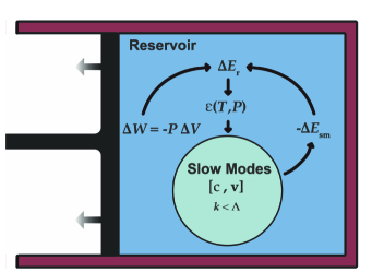
Figure 1: Our theoretical model of adiabatic decomposition in critical binary liquids. The piston (black) expands the liquid, which is contained in an insulated container (brick red). All work by the piston is done only on the reservoir (blue) subsystem of the liquid. The reservoir temperature, $T$, and pressure, equal to the external pressure, $P$, thus change. The slow mode (green-blue) subsystem of the liquid feels this change through the reduced temperature, $\epsilon(T,P)$. The slow modes then relax, changing their energy $E_{sm}\equiv{\langle{\cal E}[c,{\bf v}]\rangle}$, which is dumped back into the reservoir, causing a further change in $T$, etc.

II.2 Temperature Dependent Coarse-Grained Free Energy

The last elements of the adiabatic theory are expressions for the temperature dependent coarse-grained free energy and energy. In isothermal decomposition, ${\cal F}$ is taken to be that of Model H, which is a sum of a Cahn-Hilliard/Ginzburg-Landau free energy for the concentration field, $c({\bf r})$, and the kinetic energy of the fluid velocity field ${\bf v}({\bf r})$:

$${\cal F}[u,{\bf v}]=\int_{\Lambda}d{\bf r}\Bigl{[}{K\over 2}\bigl{(}\nabla u({\bf r})\bigr{)}^{2}+f(u({\bf r})+c_{0})+{1\over 2}\rho{\bf v}({\bf r})^{2}\Bigr{]},$$ (II.39)

where $u({\bf r})\equiv c({\bf r})-c_{0}$ with $c_{0}$ being the average concentration. Also, $f(c)$ is the free energy density of a uniform system at concentration $c$, the gradient term is the lowest order correction to the free energy from deviations of $u({\bf r})$ from zeroCahn and Hilliard (1958), and $\rho$ is the average mass density. In LBM and KO, the implicit cut-off is set to be inversely proportional to the correlation length at the quenched temperature, $T_{f}$, i.e., $\Lambda\sim 1/\xi_{f}$. Further, these theories also choose $f(c)$ to have the standard “$\varphi^{4}$” form, it being the dominant correction to the quadratic term in the critical region.Ma (2001)

Given this, follow LBM and let

$$f(c)={k_{B}T_{f}f_{1}\over\xi_{f}^{3}}\phi(x),$$ (II.40)

where

$$\phi(x)={\zeta\over 2}x^{2}+{\lambda_{4}\over 4}x^{4}.$$ (II.41)

Here, $\zeta$ and $\lambda_{4}$ are constants to be determined. Also, $x={(c-c_{c})/u_{sf}}$ is a reduced concentration, with $u_{sf}=B{|\epsilon_{f}|}^{\beta}$ being half the miscibility gap at the quenched temperature $T_{f}$, so that the scaled free energy density $\phi(x)$ is symmetric about the critical concentration. Last, $f_{1}={\xi_{f}^{3}u_{sf}^{2}/\chi_{f}}$, where $\xi_{f}$ and $\chi_{f}$ are the correlation length and susceptibility, respectively, at $T_{f}$. In the critical region hyperscaling holds,Stanley (1971) so $f_{1}={(\xi_{0}^{-})^{3}B^{2}/\Gamma^{-}}$, which is a temperature independent, dimensionless ratio of two-phase amplitudes.

Last, the gradient energy coefficient

$$K=\lambda_{K}{k_{B}T_{f}\xi_{f}^{2}\over\chi_{f}},$$ (II.42)

where $\chi_{f}=\Gamma^{-}{|\epsilon_{f}|}^{-\gamma}$ is the susceptibility at $T_{f}$, and $\lambda_{K}$ is a dimensionless number very close to unity.

How then should ${\cal F}$ be generalized to describe kinetics in which the temperature is not constant? While the early-stage theories of KO and LBM can be used for computing equilibrium states, they are not intended to describe properly static critical phenomena. In spite of this, they do incorporate fluctuations to some degree. Thus, it can be expected that these fluctuations will at least shift the apparent distance from the critical point, in a manner similar to how they shift the coexistence concentrations away from the minima of $f(c)$. So a correction for this shift in $T_{c}$ must be made in ${\cal F}$.

What will be done here is just assume a simple temperature dependent form for ${\cal F}$ and compute its coefficients. Then, the free energy will be examined to determine how well it predicts some equilibrium properties of a critical binary mixture such as the equation of state and susceptibility. If the free energy gives satisfactory results in regions important to the adiabatic decomposition theory, then its form and the scheme used to compute it will be considered adequate.

In that spirit, and given the arguments above (including those leading to Eq.(II.10)), assume that the dominant temperature dependence in the theory is in $\zeta$ and $\lambda_{4}$. The latter changes to $\lambda_{4}{T/T_{f}}$, recognizing that the $x^{4}$ term arises from the configurational entropy. The $x^{2}$ term has both entropic and energetic origins, so let $\zeta$ be linear in $\epsilon$:

$$\zeta\rightarrow\zeta(\epsilon)\approx(\lambda_{2}-\lambda_{0}){\epsilon\over|\epsilon_{f}|}-\lambda_{0}.$$ (II.43)

So, $\zeta(0)=-\lambda_{0}$ and $\zeta(\epsilon_{f})=-\lambda_{2}$, assuming $\epsilon_{f}<0$. Since the experiments are in the critical region, any other temperature or volume dependence of ${\cal F}$ will be ignored.

As $T_{c}$ itself changes when the density changes, $\epsilon$ will be a function of both $T$ and $V$. However, for a system at constrained pressure, $T_{c}$ is a function of pressure only, so $\epsilon$ will be considered a function of $T$ and $P$ rather than $T$ and $V$. In that manner, the equation of motion for $V$, Eq.(II.28), will not be used.

With Eqs.(II.10) and (II.39)-(II.43), the average coarse-grained energy ${\langle{\cal E}[c,{\bf v}]\rangle}=-\langle T^{2}\partial({\cal F}/T)/\partial T\rangle$ can be computed. In the Appendix it is shown that the heat of mixing dominates near the critical point, so

$${\langle{\cal E}[c,{\bf v}]\rangle}\approx-(\lambda_{2}-\lambda_{0}){1\over{|\epsilon_{f}|}}{f_{1}\over 2}\langle x^{2}\rangle\biggl{(}{k_{B}T_{f}V\over\xi_{f}^{3}}\biggr{)}.$$ (II.44)

The one-point average $\langle x^{2}\rangle$ can be obtained from the structure factor or one-point probability density, these quantities being the subject of the next section. The computation of the $\lambda_{i}$ parameters will be described in Sec. V below.

The theoretical model of adiabatic decomposition given here is summarized in Figure 1.

III Kawasaki-Ohta Theory

As mentioned above, the KO/LBM theory of early-stage decomposition will be used to compare with experiment. This section describes the theory briefly.

KO is considered to be the most successful numerical theory of decomposition in critical binary fluids. It, like LBM, is built upon the theory of stochastic processes.N. G. Van Kampen (2007) The KO theory consists of a set of equations that describe the time evolution of the structure factor ${\hat{S}}(k,t)$, where $k\equiv|{\bf k}|$ is the wavevector. Contact with experiment is made by relating ${\hat{S}}(k,t)$ to the scattered radiation intensity $I(k,t)$.Bailey and Cannell (1994)

Now, let $u_{\bf k}$ be the Fourier transform of the concentration deviation $u({{\bf r}})$. The structure factor ${\hat{S}}(k)$ is defined as

$${\hat{S}}(k)=\langle|u_{\bf k}|^{2}\rangle,$$ (III.1)

and is the Fourier transform of the concentration-concentration correlation function

$$S({{\bf r}}-{{\bf r}}_{0})=\langle u({{\bf r}})u({{\bf r}}_{0})\rangle.$$ (III.2)

This function can be obtained from theory by taking moments of $\rho([u],t)$, which, as mentioned above, is the probability density that the system is in a coarse-grained configuration $[u]$ at time $t$.

In KO theory, the time evolution of the probability density $\rho([u],t)$ is determined by a Fokker-Planck equation Kawasaki and Ohta (1978):

$${\partial\rho\over\partial t}=\Bigl{[}{\cal L}_{1}+{\cal L}_{2}\Bigr{]}\rho,$$ (III.3)

where the operators are given by

$${\cal L}_{1}=-\int d{{\bf r}}_{1}d{{\bf r}}_{2}{\delta\over\delta u({{\bf r}}_{1})}\nabla_{1}^{2}L_{\Lambda}({{\bf r}}_{1}-{{\bf r}}_{2})\Bigl{[}{\delta{\cal F}\over\delta u({{\bf r}}_{2})}+k_{B}T{\delta\over\delta u({{\bf r}}_{2})}\Bigr{]},$$ (III.4)

and

$${\cal L}_{2}=\int d{{\bf r}}_{1}d{{\bf r}}_{2}{\delta\over\delta u({{\bf r}}_{1})}\nabla_{1}u({{\bf r}}_{1})\cdot{\bf T}({{\bf r}}_{1}-{{\bf r}}_{2})\cdot\nabla_{2}u({{\bf r}}_{2})\Bigl{[}{\delta{\cal F}\over\delta u({{\bf r}}_{2})}+k_{B}T{\delta\over\delta u({{\bf r}}_{2})}\Bigr{]}.$$ (III.5)

Here, ${\delta/\delta u({\bf r})}$ is a functional derivative with respect to the concentration field at the point ${\bf r}$, and ${\bf T}({\bf r})$ is the Oseen tensor with components $T_{\alpha\beta}=[\delta_{\alpha\beta}+{\hat{r}}_{\alpha}{\hat{r}}_{\beta}]/(8\pi\eta_{s}r)$, with $\eta_{s}$ being the hydrodynamic shear viscosity and ${\hat{r}}\equiv{{\bf r}/r}$.

Eqs. (III.3-III.5) describe phase separation driven by incompressible, overdamped fluid flow, the flow in turn caused by gradients in the local chemical potential, $\mu({\bf r})={\delta{\cal F}[u]/\delta u({\bf r})}$. These equations are renormalized versionsKawasaki (1977) of bare stochastic equationsKawasaki (1973), which are formally equivalent to the Langevin equations of Model H of critical dynamicsHohenberg and Halperin (1977) in the overdamped approximation, i.e., ${\bf v}={\bf T}\cdot(\mu\nabla u+{\rm noise})$.

The operator ${\cal L}_{1}$ results from integrating out concentration fluctuations of wavenumber $k>\Lambda$. The Onsager function $L_{\Lambda}(r)$ that appears in ${\cal L}_{1}$ is weakly non-local and couples these short-wavelength concentration modes, $\it via$ the fluid velocity field, to the long-wavelength modes $k<\Lambda$. $L_{\Lambda}(r)$ is the inverse Fourier transform of Kawasaki (1977):

$${\hat{L}_{\Lambda}}(k_{1})={1\over k_{1}^{2}}\int{d{\bf k}_{2}\over(2\pi)^{3}}{\bf k}_{1}\cdot{\bf\hat{T}}({\bf k}_{1}-{\bf k}_{2})\cdot{\bf k}_{1}{\hat{S}}_{eq}(k_{2}).$$ (III.6)

Here, the integral over $k_{2}$ runs from $\Lambda$ to an upper cut-off which is approximated as infinity. ${\bf\hat{T}}({\bf k})$ is the Fourier transform of the Oseen tensor with components $[\delta_{\alpha\beta}-{\hat{k}}_{\alpha}{\hat{k}}_{\beta}]/(\eta_{s}k^{2})$. ${\hat{S}}_{eq}(k)$ is the equilibrium structure factor of mode $k\ (>\Lambda)$, and is taken to have a Lorentzian form:

$${\hat{S}}_{eq}(k)={\chi\over 1+(k\xi)^{2}},$$ (III.7)

where $\chi$ and $\xi$ are the susceptibility and correlation length, respectively, at temperature $\epsilon$ and concentration $c_{0}$. Clearly, as the temperature changes, ${\hat{S}}_{eq}(k)$, and therefore ${\hat{L}_{\Lambda}}(k)$, will be changing also. However, it can be shown Kawasaki (1977) that a reasonable approximation to Eq. (III.6) is

$${\hat{L}_{\Lambda}}\simeq{\chi\over 3\pi^{2}\xi^{2}\eta_{s}\Lambda}.$$ (III.8)

Making use of Tables 1 and 2 for $\chi,\xi$ and $\eta_{s}$, it is found that ${\hat{L}_{\Lambda}}$ has a weak temperature dependence. Thus, if the quenches are relatively fast, ${\hat{S}}_{eq}(k)$ can be set to its value at the final equilibrium temperature $\epsilon_{f}$. Further, the weak temperature dependence of the viscosity $\eta_{s}$ will also be ignored. Then with these approximations, the only temperature dependence in (III.3) appears in the coarse-grained free energy, ${\cal F}[c,{\bf v}]$.

An equation of motion for the structure factor ${\hat{S}}(k,t)$ was derived by KO using Eqs. (II.39) and (III.3-III.6). To evaluate two-point correlation functions in ${\cal L}_{1}$ other than $S(r)$, they used the LBM self-consistent, first order expansion for the two-point probability density:

$$\rho_{2}^{lbm}(u_{1},u_{2})=\rho_{1}(u_{1})\rho_{1}(u_{2})\Bigl{[}1+{u_{1}u_{2}\over\langle u^{2}\rangle^{2}}S(r_{12})\Bigr{]},$$ (III.9)

where $r_{12}\equiv|{\bf r}_{1}-{\bf r}_{2}|$, $u_{1}\equiv u({\bf r}_{1})$, etc. This approximation is expected to work best during the early stage of decomposition when the growing domains are not much larger than a few equilibrium correlation lengths and sharp interfaces have not yet formed.Langer et al. (1975) Implicit in the LBM derivation is an important constraint that averages taken with respect to $\rho_{2}$ must reduce to their exact form in the limit $r_{12}\rightarrow 0$. That is, for arbitrary functions $h(u)$ and $g(u)$, $\langle h(u_{1})g(u_{2})\rangle\rightarrow\langle h(u)g(u)\rangle$ as $r_{12}\rightarrow 0$, where the latter average is taken with respect to the one-point probability density $\rho_{1}(u)$. Implementing this constraint in a simple way, and using the LBM approximation above, gives an equation for $\rho_{2}$:

$$\rho_{2}(u_{1},u_{2})\approx \rho_{2}^{lbm}(u_{1},u_{2})+a^{3}\delta({\bf r}_{1}-{\bf r}_{2})\Bigl{[}$$

$$\rho_{1}(u_{1})\delta(u_{1}-u_{2})-\rho_{2}^{lbm}(u_{1},u_{2})\bigr{|}_{r_{12}\rightarrow 0}\Bigr{]}.$$

The ${\cal L}_{2}$ contribution to ${\hat{S}}(k,t)$ contains a four-point correlation function. KO argued that during the early stage of decomposition the coupling between modes in this correlation function would be close to gaussian. In this approximation the four-point correlation function reduces to a product of two-point ones.Kawasaki and Ohta (1978)

The result is:

$${\partial{\hat{S}}(k_{1})\over\partial t} =-2{\hat{L}_{\Lambda}}(k_{1})k_{1}^{2}\Bigl{[}\bigl{(}Kk_{1}^{2}+A\bigr{)}{\hat{S}}(k_{1})-k_{B}T\Bigr{]}$$ (III.11)

$$+ 2\int^{\Lambda}{d{\bf k}_{2}\over(2\pi)^{3}}{{\bf k}_{1}}\cdot{\bf\hat{T}}({\bf k}_{1}-{\bf k}_{2})\cdot{{\bf k}_{1}}$$

$$\times\Bigl{[}K\bigl{(} k_{2}^{2}-k_{1}^{2}\bigr{)}{\hat{S}}(k_{2}){\hat{S}}(k_{1})+k_{B}T{\hat{S}}(k_{2})-k_{B}T{\hat{S}}(k_{1})\Bigr{]}.$$

Here,

$$A={1\over\langle u^{2}\rangle}\bigl{\langle}u{\partial f(u+c_{0})\over\partial u}\bigr{\rangle},$$ (III.12)

where the averages are taken with respect to $\rho_{1}(u)$.

It can be shownKawasaki and Ohta (1978) that the operator ${\cal L}_{2}$ doesn’t contribute directly to the equation of motion for $\rho_{1}(u)$. Given this, the derivation of the equation of motion for $\rho_{1}(u,t)$ from Eq.(III.3) is almost identical to the one in LBM. It is found:

$${\partial\rho_{1}(u)\over\partial t}={\partial\over\partial u}\Bigl{[}G(u)\rho_{1}(u)+k_{B}T{L\over a^{3}}{\partial\rho_{1}(u)\over\partial u}\Bigr{]},$$ (III.13)

where

$$G(u)=W{u\over\langle u^{2}\rangle}+L\Bigl{[}{\partial f\over\partial u}-\bigl{\langle}{\partial f\over\partial u}\bigr{\rangle}-uA\Bigr{]},$$ (III.14)

$$W=\int_{0}^{\Lambda}{dk\over 2\pi^{2}}k^{4}{\hat{L}_{\Lambda}}(k)\bigl{(}Kk^{2}+A){\hat{S}}(k),$$ (III.15)

and

$$L=a^{3}\int_{0}^{\Lambda}{dk\over 2\pi^{2}}k^{4}{\hat{L}_{\Lambda}}(k).$$ (III.16)

For the initial conditions of these equations, the equilibrium solution of them will be used. Setting the RHS of Eq.(III.13) to zero yields:

$$\rho_{1eq}(u) =exp\Bigl{[}-{u^{2}\over 2\langle u^{2}\rangle}+b_{0}$$ (III.17)

$$- {a^{3}\over k_{B}T}\bigl{(}f(u+c_{0})-u\mu-{u^{2}\over 2}A\bigr{)}\Bigr{]}$$

where $b_{0}$ is a normalization constant, and $\mu\equiv\langle{\partial f/\partial u}\rangle$ is the chemical potential. Both $\mu$ and $A$ are determined self-consistently, while $\langle u^{2}\rangle=S(0)$ is an input obtained from the Fourier transform of the structure factor. The equilibrium structure factor is found by setting the RHS of Eq.(III.11) to zero, giving

$${\hat{S}}_{eq}(k)={k_{B}T\over Kk^{2}+A}.$$ (III.18)

These kinetic and equilibrium equations were solved numerically.

IV Scaling and Numerical Solution

IV.1 Scaling of the Equations

For numerical computation, it is helpful to scale the above equations. While in adiabatic decomposition the temperature will necessarily be changing with time after the quench, the final equilibrium temperature will still be the relevant one. So, as in KO and LBM, the scaling will be done with respect to system properties at $\epsilon_{f}$.

Define the scaled wavevector cut-off $\alpha^{\ast}=\Lambda\xi_{f}$, where $\alpha^{\ast}$ is a number close to 1. Define also the dimensionless wavevector, $q=k\xi_{f}$; distance, ${\tilde{r}}=r/\xi_{f}$; structure factor, ${\tilde{S}}(q)={\hat{S}}(k)/\chi_{f}$; relative concentration, $y=u/u_{sf}$; average concentration, $x_{0}={(c_{0}-c_{c})/u_{sf}}$; and time, $\tau=k_{B}T/(6\pi\eta_{s}\xi_{f}^{3})t$. As for LBM, the cell volume $a^{3}=(\int{d{\bf k}}/(2\pi^{3}))^{-1}={6\pi^{2}\xi_{f}^{3}/(\alpha^{\ast})^{3}}$.

It is convenient to scale the Onsager function, Eq.(III.6), as

$$\sigma(q)= {6\pi\xi_{f}\eta_{s}\over\chi_{f}}{\hat{L}_{\Lambda}}(q/\xi_{f})$$ (IV.1)

$$= K(q)-{3\over 2\pi}\int_{0}^{\alpha^{\ast}}dm\ Q(q/m){1\over 1+m^{2}}$$

where $K(q)$ is a Kawasaki functionKawasaki and Ohta (1978):

$$K(q)={3\over 4}\Bigl{[}({1\over q}-{1\over q^{3}})\arctan(q)+{1\over q^{2}}\Bigr{]},$$ (IV.2)

and

$$Q(x)={1\over 2}\Bigl{[}{1\over x}+{1\over x^{3}}\Bigr{]}{\rm ln}\bigl{|}{1+x\over 1-x}\bigr{|}-{1\over x^{2}}.$$ (IV.3)

Changing to the new scaled variables and performing any angular integration, the equation of motion for the structure factor becomes:

$${\partial{\tilde{S}}(q)\over\partial\tau} =-2\sigma(q)q^{2}\Bigl{[}(\lambda_{K}q^{2}+{\tilde{A}}){\tilde{S}}(q)-1\Bigr{]}$$ (IV.4)

$$+ {3\over\pi}q^{2}\int_{0}^{\alpha^{\ast}}dm\ Q(q/m)$$

$$\times\Bigl{[} \lambda_{K}(m^{2}-q^{2}){\tilde{S}}(q){\tilde{S}}(m)+{\tilde{S}}(m)-{\tilde{S}}(q)\Bigr{]},$$

where

$${\tilde{A}}={1\over\langle y^{2}\rangle}\bigl{\langle}y{\partial\phi(y+x_{0})\over\partial y}\bigr{\rangle}.$$ (IV.5)

The kinetic equation for the one-point probability density $\rho_{1}$ is now

$${\partial\rho_{1}(y)\over\partial\tau}=\omega{\partial\over\partial y}\Bigl{[}g(y)\rho_{1}(y)+{\partial\rho_{1}(y)\over\partial y}\Bigr{]},$$ (IV.6)

where

$$\omega={1\over f_{1}}\int_{0}^{\alpha^{\ast}}{dq\over 2\pi^{2}}q^{4}\sigma(q),$$ (IV.7)

and

$$g(y)={{\tilde{W}}y\over\langle y^{2}\rangle}+f_{0}\Bigl{[}{\partial\phi\over\partial y}-\langle{\partial\phi\over\partial y}\rangle-y{\tilde{A}}\Bigr{]},$$ (IV.8)

with

$${\tilde{W}}={1\over f_{1}\omega}\int_{0}^{\alpha^{\ast}}{dq\over 2\pi^{2}}\ q^{4}\sigma(q)(\lambda_{K}q^{2}+{\tilde{A}}){\tilde{S}}(q).$$ (IV.9)

Here, $f_{0}={6\pi^{2}f_{1}/(\alpha^{\ast})^{3}}$.

Last, using Eq.(II.27), it can be found that the equation of motion for the reduced temperature is:

$${d\epsilon\over d\tau}=\Bigl{[}{\alpha_{Pr}\over\rho_{c}C_{Pr}}-{1\over T_{c}}{dT_{c}\over dP}\Bigr{]}{dP\over d\tau}-{k_{B}\over\xi_{f}^{3}\rho_{c}C_{Pr}}{d{\tilde{e}}\over d\tau},$$ (IV.10)

where $\rho_{c}$ is the critical mass density and $C_{Pr}$ is now the reservoir heat capacity per unit mass, and the average coarse-grained energy, Eq. (II.44), properly scaled, is:

$${\tilde{e}}= {\xi_{f}^{3}\over Vk_{B}T_{f}}\langle{\cal E}[c,{\bf v}]\rangle$$

$$= -(\lambda_{2}-\lambda_{0}){f_{1}\over 2{|\epsilon_{f}|}}\langle x^{2}\rangle.$$ (IV.11)

The scaled form of the equilibrium equations, (III) and (III.18), are, respectively,

$$\rho_{1eq}(y) =exp\Bigl{[}-{y^{2}\over 2\langle y^{2}\rangle}+b_{0}$$ (IV.12)

$$- f_{0}\bigl{(}\phi(y+x_{0})-y\langle{\partial\phi\over\partial y}\rangle-{y^{2}\over 2}{\tilde{A}}\bigr{)}\Bigr{]},$$

and

$${\tilde{S}}_{eq}(q)={1\over\lambda_{K}q^{2}+{\tilde{A}}},$$ (IV.13)

where again $b_{0}$ is a normalization constant.

From these equations it can be seen that an (linear) isothermal quench and subsequent decomposition is completely specified by the quench time $\tau_{quench}$, the ratio of the initial to the final scaled temperature, $\epsilon_{i}/\epsilon_{f}$, and the average concentration $x_{0}$. In addition to the properties of the particular fluid one wants to study, an adiabatic quench is completely specified by these same quantities plus the change in pressure, $\Delta P$. The predictions of the theory are also somewhat dependent on the value of the scaled cut-off $\alpha^{\ast}$. However, the degree of this dependence will be minimized by the method of computing the $\lambda_{i}$ parameters in the coarse-grained free energy, discussed below.

IV.2 Numerical Solution

The scaled adiabatic equations were solved numerically as follows.

${\tilde{S}}(q)$ was solved on a grid of $N_{q}$ points $q_{i}=i\Delta q$, $i=1,...,N_{q}$ in $q$-space, with spacing $\Delta q=2\alpha^{\ast}/N_{q}$. ${\tilde{S}}(q)$ was set to zero for all grid points $q_{i}>\alpha^{\ast}$. The reason the grid was extended in this manner was to be able to inverse Fourier transform ${\tilde{S}}(q)$ if need be. The $q$ grid point number $N_{q}$ was set to $2^{9}=512$ for any run with a maximum time $\tau_{max}\leq 10^{3}$, and was set to $2^{10}=1024$ for longer runs of $10^{3}<\tau_{max}\leq 10^{4}$. Similarly, $\rho_{1}(y)$ was solved on a grid of $N_{y}$ equally spaced points $y_{i}$, $i=1,..,N_{y}$ in $y$-space, with $y_{1}=y_{min}+\Delta y/2$, $y_{2}=y_{min}+3/2\Delta y$, and $y_{N_{y}}=y_{max}-\Delta y/2$, where $\Delta y=N_{y}/(y_{max}-y_{min})$ and $y_{min}=-y_{max}$. To ensure that $\rho_{1}(y)$ could model properly behavior near the coexistence curve at $\epsilon_{f}$, $y_{max}$ was set to 2.5. Also, $N_{y}=120$ for all results shown in this work. It was found that no result shown here changed appreciably if $N_{q}$ and $N_{y}$ were increased beyond the above values.

Now, the adiabatic theory consists of ODE’s for ${\tilde{S}}(q,\tau)$ and $\epsilon(\tau)$, and a PDE for $\rho_{1}(y,\tau)$. To simplify the computation, the PDE for $\rho_{1}(y,\tau)$ was converted into a set of coupled ODE’s, using a simple finite difference scheme. Let $\rho_{1i}$ and $g_{i}$ be the values of $\rho_{1}(y)$ and $g(y)$ at the $i$th grid point $y_{i}$. Then, Eq. (IV.6) becomes

$${d\rho_{1i}\over d\tau} =\omega\Bigl{[}g_{i+1}\rho_{1(i+1)}-g_{i-1}\rho_{1(i-1)}\Bigr{]}/(2\Delta y)$$

$$+ \omega\Bigl{[}\rho_{1(i+1)}+\rho_{1(i-1)}-2\rho_{1i}\Bigr{]}/\Delta y^{2},$$ (IV.14)

with the boundary conditions $\rho_{11}=\rho_{1N_{y}}=0$. A total of $N=N_{q}/2+N_{y}-2+1$ ODE’s result. The integration of these in time was done using the Bulirsch-Stoer method.Press et al. (1992) The structure factor equations are stiff in the sense that the relaxation of the high-$q$ modes is much faster than the low-$q$ ones. The Bulirsch-Stoer method is not usually used for solving such an ODE type. Given that, initially the equations were also solved using a commercial package built for solving stiff ODE’s.NAG (1 27) It was found that both methods yielded the same results.

In past work, the PDE for $\rho_{1}(y)$ was solved instead using the much faster “double gaussian” method.Langer et al. (1975) This method was analyzed for on-critical quenches, $x_{0}=0$, and found to give essentially identical results to the finite difference method at early times. However, it over-estimated the phase separation at later times when the wavevector $q_{m}$ of the peak of the structure factor was less than $0.3$. For the BC experiments, data was available out to times such that $q_{m}<0.2$. As a consequence, this approximation was not used here.

For each timestep, $\rho_{1}$ was normalized to prevent accumulation of round-off errors. The first moment, $\langle y\rangle$ of $\rho_{1}$ was monitored to ensure that it remained zero. The integral of ${\tilde{S}}(q)$ and $\rho_{1}$ were also monitored to ensure that they gave the same result for $\langle y^{2}\rangle$.

The equilibrium equations, (IV.1) and (IV.13), were solved using the same grids for $q$ and $y$, though here $N_{q}$ was set to $2^{12}=4096$. Simple iteration was used for them. The initial guess for ${\tilde{S}}_{eq}(q)$ was a scaled version of Eq.(III.7) at the relevant initial $\epsilon$ and $x_{0}$. However, if the LBM solution of ${\tilde{S}}_{eq}(q)$ differed appreciably from the known value, bootstrap, i.e., a previous guess at a nearby temperature and concentration, was used instead.

V Computing the Coarse-Grained Free Energy

The last ingredients of the theory are values for the $\lambda_{i}$ parameters in the coarse-grained free energy, defined in Sec. II.2 above. Similar to LBM, these parameters were determined by using ${\cal F}$ to compute the equilibrium structure factor and chemical potential on coexistence at the final temperature $\epsilon_{f}$, and at the critical point $\epsilon=0$. There are a number of ways to accomplish this task. The one probably most accurate for the least amount of effort is to use the LBM equilibrium solution for ${\tilde{S}}(q)$ and $\rho_{1}(y)$.Billotet and Binder (1979) This scheme was used here. It amounts to applying $N$ equilibrium conditions to the LBM equations for the $N$ unknowns, and finding the solution of them using the Newton-Raphson method.Press et al. (1992) Here, all derivatives required by this method were computed numerically.

For here and elsewhere in this work, the free energy amplitude $f_{1}$ was set to 0.210, consistent with the critical amplitude values in Table 2.

On coexistence, $\epsilon=\epsilon_{f}$ and $x_{0}=1$, the scaled equilibrium structure factor ${\tilde{S}}(q)=1/(1+q^{2})$. Two relations obtained from this equation were ${\tilde{S}}(0)=1$ and

$$\langle y^{2}\rangle= {1\over 2\pi^{2}f_{1}}\int_{0}^{\alpha^{\ast}}dqq^{2}{\tilde{S}}(q)$$

$$= {1\over 2\pi^{2}f_{1}}\bigl{[}\alpha^{\ast}-\arctan(\alpha^{\ast})\bigr{]}.$$ (V.1)

A third relation is that the exchange chemical potential must vanish on coexistence: ${\tilde{\mu}}=\langle{\partial\phi/\partial x}\rangle=0$. These three equations are sufficient to determine $\lambda_{K}$, $\lambda_{2}$ and $\lambda_{4}$ for any cut-off $\alpha^{\ast}$. The last parameter $\lambda_{0}$ was determined by requiring that ${\tilde{S}}(0)=\infty$, i.e., $\tilde{A}=0$, at the critical point, $\epsilon=0$ and $x_{0}=0$. Values for the $\lambda_{i}$ parameters for various cut-offs are shown in Table 3 below. Note that the value of $\lambda_{0}$ does not depend on the form of the temperature dependence of $\zeta$, Eq.(II.43), only that it reduce to $-\lambda_{0}$ at $\epsilon=0$.

Table 3: Coarse-grained free energy coefficients $\lambda_{i}$ for various wavevector cut-offs $\alpha^{\ast}$.

$\alpha^{*}$	$\lambda_{K}$	$\lambda_{0}$	$\lambda_{2}$	$\lambda_{4}$
1.0	1.0	0.3203	0.6915	0.6020
1.4	1.0	0.5169	0.8734	0.6704
$\pi/2$	1.0	0.6054	0.9533	0.6913

To justify some approximations made previously, it is helpful to examine the predictions of the equilibrium LBM theory on-critical above $T_{c}$ and on-coexistence below it.

Figure 2 shows LBM predictions for the equilibrium, on-critical inverse susceptibility ${\tilde{S}}^{-1}(0)$ as a function of ${\epsilon/|\epsilon_{f}|}>0$ for two cutoff values $\alpha^{\ast}=1$ and $\pi/2$. Also shown are the expected scaling predictions for a simple binary fluid (3-D Ising universality class): ${\tilde{S}}(0)^{-1}=\Gamma^{-}/\Gamma^{+}|{\epsilon/\epsilon_{f}}|^{\gamma}$ where the amplitude ratio and exponent are obtained from Table 2. For ${\epsilon/|\epsilon_{f}|}\ll 1$, it is found that LBM also predicts scaling behavior, with the exponent $\gamma$ approximately equal to the mean spherical model value of 2.Stanley (1971) Since the accepted 3-D Ising value of $\gamma\approx 1.240$, the LBM theory does not perform well in this limit as expected. However, it can seen for higher temperatures the theory performs much better. For $0.5\leq{\epsilon/|\epsilon_{f}|}\leq 10$, the LBM predictions for ${\tilde{S}}(0)$ are within 10% and 20% of the exact values for $\alpha^{\ast}=1$ and $\alpha^{\ast}=\pi/2$, respectively. For higher temperatures, the agreement lessens, but ${\tilde{S}}(0)$ is small there anyways. It was found that the predictions of the hydrodynamic theory are pretty much insensitive to such small variations in the initial conditions. (More important is that ${\tilde{S}}(q)$ and $\rho_{1}(y)$ be consistent with each other.)

Define an effective susceptibility exponent

$$\gamma_{eff}=-ln\bigl{[}{\tilde{S}}(0,\epsilon_{1})/{\tilde{S}}(0,\epsilon_{2})\bigr{]}/ln\bigl{[}\epsilon_{1}/\epsilon_{2}\bigr{]},$$ (V.2)

where the temperatures $\epsilon_{1}$ and $\epsilon_{2}$ are close to each other in some sense. Then, over this temperature range, $0.5\leq{\epsilon/|\epsilon_{f}|}\leq 10$, LBM predicts that $\gamma_{eff}$ varies from 1.39 down to 1.10 for $\alpha^{\ast}=1$, and 1.47 down to 1.15 for $\alpha^{\ast}=\pi/2$. Also, for $\alpha^{\ast}=1$ and ${\epsilon/|\epsilon_{f}|}=1.5$, and $\alpha^{\ast}=\pi/2$ and ${\epsilon/|\epsilon_{f}|}=2.3$, $\gamma_{eff}=1.24$, i.e., is exact.

Thus, the LBM theory seems to describe properly the temperature dependence of critical fluctuations within a window near ${\epsilon/|\epsilon_{f}|}=1$. It is concluded then that using the equilibrium LBM theory, along with ${\cal F}$ defined in Sec. II.2 above, to give initial conditions for ${\tilde{S}}(q)$ and $\rho_{1}(y)$ is acceptable as long as the quenches are not too deep, ${\epsilon/|\epsilon_{f}|}>0.5$.

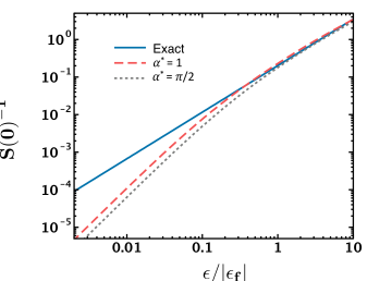
Figure 2: LBM predictions, using the temperature dependent coarse-grained free energy defined in Sec. II.2, for the equilibrium, one-phase, on-critical, inverse susceptibility ${\tilde{S}}(0)^{-1}$ as a function of the scaled temperature ${\epsilon/|\epsilon_{f}|}>0$. Results for two cut-offs $\alpha^{\ast}$ are shown, along with “exact” scaling values.

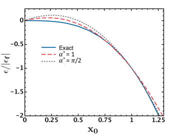
Figure 3: LBM predictions, using the temperature dependent coarse-grained free energy defined in Sec. II.2, for the coexistence curve $\epsilon(x_{0})$ for two cut-offs $\alpha^{\ast}$. Also shown is the “exact” scaling form in the critical region, ${\epsilon/|\epsilon_{f}|}=-x_{0}^{1/\beta}$, where $\beta\approx 0.33$.

Examining the LBM predictions for the two-phase coexistence curve $\epsilon(x_{0})$ is also illuminating. Figure 3 shows $\epsilon(x_{0})$ for positive $x_{0}$ (the curve is symmetrical about $x_{0}=0$) for cutoffs $\alpha^{\ast}=1$ and $\pi/2$. Also shown is the accepted scaling form for a system in the 3-D Ising universality class: $\epsilon(x_{0})\sim-|x_{0}|^{1/\beta}$, with $\beta\approx 0.33$. Thus, $\epsilon(x_{0})$ should have a maximum at $x_{0}=0$. However, as can be seen, instead of a maximum at $x_{0}=0$, the LBM predictions overshoot $\epsilon=0$ and have a maximum at around $x_{0}=0.2$ and $0.25$ for $\alpha^{\ast}=1$ and $\pi/2$, respectively. Thus, the LBM theory should not be used to describe the initial state for quenches that are deep, ${\epsilon/|\epsilon_{f}|}\ll 1$, and off-critical. Also, contrary to its behavior above $T_{c}$, the LBM predictions for $\gamma_{eff}$ below $T_{c}$ are always below the accepted 3-D Ising scaling value of $1.240$, at best reaching $0.9$ at ${\epsilon/|\epsilon_{f}|}=-2.0$.

On the other hand, the theory’s predictions for an effective $\beta$ exponent, $\beta_{eff}$, defined analogously to $\gamma_{eff}$ in Eq. (V.2) above, are near the accepted 3-D Ising value for temperatures near $\epsilon_{f}$. For $\alpha^{\ast}=1$ and ${\epsilon/|\epsilon_{f}|}=-0.85$, and $\alpha^{\ast}=\pi/2$ and ${\epsilon/|\epsilon_{f}|}=-1$, $\beta_{eff}$ equals the accepted $\beta$ value of $0.328$. Also, for temperatures near $\epsilon_{f}$, the predictions of LBM for $\epsilon(x_{0})$ are in good agreement with the accepted values in the range $-2.0\leq{\epsilon/|\epsilon_{f}|}\leq-0.5$. As will be seen below, the adiabatic theory predicts that the temperature undershoot after an on-critical quench of 3MP+NE does not go below $-2\epsilon_{f}$. Thus, if the quenches are fast, the on-coexistence equilibrium predictions of the LBM theory should be acceptable.

It is concluded that if the quenches are not too deep, and are fast enough so that the fluid spends little time exploring the region near $T_{c}$, then the temperature dependent coarse-grained free energy defined in Sec. II.2 is adequate.

VI Results

In this section, general predictions of the adiabatic and isothermal decomposition theories are discussed, and then the theories are compared with experiment. In an unpublished work, Schwartz showed that the original numerical scheme of KO was not quite right,Schwartz (1978) leading to erroneous results for the structure factor at intermediate and late times. Given this, aspects of the isothermal KO theory by itself will also be discussed.

VI.1 General Predictions

In the isothermal decomposition theory, the equations scale completely. That is, no system or temperature dependent parameter appears in the theory when the equations are scaled using parameters appropriate to the critical region. Thus, if initial (and quench) conditions are ignored, the theory predicts that if the experimental data is appropriately rescaled then the data should superimpose for any binary fluid and any quench temperature.

However, the adiabatic theory does not scale. The parameters appearing in the equation for $\epsilon$, (IV.10), are strongly system dependent and some, $\alpha_{P}$ and $C_{P}$, are temperature dependent. To illustrate the adiabatic results in this section then, data for 3MP+NE will just be used. The equation for $\epsilon$ requires $\alpha_{P},C_{P},\rho_{c},T_{c},dT_{c}/dP$ and $\xi_{0}^{\pm}$, which, for 3MP+NE, can be obtained from Tables 1 and 2.

The other parameters appearing in the theory are the universal amplitude $f_{1}$, the cut-off $\alpha^{\ast}$, and the cut-off dependent free energy parameters $\lambda_{i}$. As mentioned above, $f_{1}$ was set to 0.210, and in Sec. V values for the $\lambda_{i}$ were computed for various cut-off values. What remains then is to determine an appropriate cut-off.

In isothermal decomposition, $\alpha^{\ast}$ is determined by requiring that it be large enough so that no unstable modes are integrated out. In the mean-field theory of Cahn,Cahn (1968) the dominant unstable wavevector is at $q={1/{\sqrt{2}}}$, with the largest unstable mode occurring at $q=1$. Thus, $\alpha^{\ast}\geq 1$. While the statistical theory here gives free energy parameters that are cut-off dependent, this relation roughly holds here too.

On the other hand, the time dependent inverse susceptibility, $A(t)$, appearing in the equation of motion for the structure factor, Eq.(III.11) does not vary with the wavevector $k$ of the mode. In other words, the LBM ansatz produces a mean-field form for this time dependent inverse susceptibility.Langer et al. (1975) The goal then should be to include as few concentration modes as possible into this mean-field approximation, that is, to make $\alpha^{\ast}$ as small as possible. A good compromise between these opposing needs is to follow LBM and just let $\alpha^{\ast}=1$ for isothermal decomposition.

In adiabatic decomposition, the wavevector of the largest unstable mode will depend upon the degree of temperature undershoot. What has been done here is set $\alpha^{\ast}$ and then examine the temperature undershoot at a short time after the end of the quench, say, $\tau=0.1$. The inverse of the equilibrium correlation length for that temperature at that time was then identified to be the minimum cut-off value, in analogy with the isothermal case. For the quenches considered here, it was found that setting $\alpha^{\ast}=1.4$ was reasonable. For consistency, this cut-off was also used for the isothermal runs.

With the parameters in the equations determined, a quench is specified by the initial reduced temperature $\epsilon_{i}$, the pressure change $\Delta P$, and the quench time $\tau_{quench}$. The final temperature was determined by integrating Eq. (II.35). The quench time varied with experiment, but was either known or could be deduced.

Figure 4 shows the scaled temperature, ${\epsilon/|\epsilon_{f}|}$ as a function of the scaled time $\tau$ for three adiabatic runs ending at the temperatures $T_{c}\epsilon_{f}=-0.04$ mK, $-0.4$ mK and $-4.0$ mK, with initial temperatures $\epsilon_{i}=-10\epsilon_{f}$. The quenches were on-critical so $x_{0}=0$. The scaled quench time $\tau_{quench}$ has been set to be $0.01$; thus the initial temperature drop does not appear on the graph. Clearly, the temperature undershoot is large; the temperature reached immediately after the quench is roughly $-1.8|\epsilon_{f}|$, with the smaller final temperatures giving the greater undershoot. As can be seen, there is a sharp rise from this minimum at early times $\tau<5$, and then a gradual rise later. This qualitative behavior has been seen by Milchev et al. in a 2-D Ising simulation of adiabatic decomposition.Milchev et al. (1994) Note also that there is not much difference in the scaled temperature trajectories even though the final scaled temperatures differ by a factor of 100.

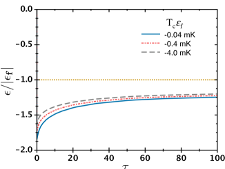
Figure 4: Scaled temperature $\epsilon/|\epsilon_{f}|$ as a function of scaled time $\tau$ for three adiabatic runs. The final temperatures $T_{c}\epsilon_{f}$ are indicated in the figure and the initial temperatures are $\epsilon_{i}=-10\epsilon_{f}$. The straight line denotes the final equilibrium temperature.

Figures 5 and 6 show results for the scaled peak intensity, ${\tilde{S}}(q_{m})$, and scaled peak wavevector, $q_{m}$ as functions of the scaled time $\tau$. Results of the middle adiabatic quench in Figure 4, $T_{c}\epsilon_{f}=-0.4$ mK, are shown along with results from an isothermal run with the same ratio of $\epsilon_{i}/\epsilon_{f}=-10$. Also shown are results from an “LBM” version of the theory in which $\sigma(q)$, Eq.(IV.1), is set to 1 and the second term in Eq. (IV.4) due to the hydrodynamic operator ${\cal L}_{2}$ is dropped. Setting $\sigma(q)=1$ assumes all modes have equilibrated, which clearly is not the case, so that value should be considered an upper bound. In Figure 5 it can be seen that the temperature undershoot causes ${\tilde{S}}(q_{m})$ for the adiabatic quench to grow initially more rapidly than the isothermal quench.

Interestingly, ${\tilde{S}}(q_{m})$ for the adiabatic quench in Figure 5 never differed from the peak height of the other two adiabatic quenches in Figure 4 (not shown) by more than about $5\%$ at late times even though there is a spread of two orders of magnitude in their final temperatures. This weak violation of scaling is caused by the weak divergence ($\alpha=0.105$) of $\alpha_{P}$ and $C_{P}$. On the other hand, ${\tilde{S}}(q_{m})$ for the isothermal quench differs by at least a factor of 2 from the adiabatic runs. At very early times, the LBM prediction is greater than either version of the KO theory, due presumably to the overestimation of the transport function $\sigma(q)$. At later times, LBM lags appreciably behind KO as expected.

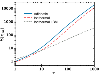
Figure 5: Scaled structure factor peak ${\tilde{S}}(q_{m})$ as a function of scaled time $\tau$ for an adiabatic and isothermal run of the KO theory. Also shown are predictions of an isothermal run from an LBM version of the theory. The adiabatic run is the same as the middle one in Fig.4: $T_{c}\epsilon_{f}=-0.4$ mK and $\epsilon_{i}/\epsilon_{f}=-10$; the isothermal runs have the same ratio of initial to final temperature. Results for adiabatic runs for other temperatures shown in Fig.4 gave peak values that differed at most by $5\%$ from the $T_{c}\epsilon_{f}=-0.4$ mK run here.

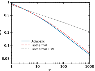
Figure 6: Scaled peak wavevector $q_{m}$ as a function of scaled time $\tau$ for an adiabatic and isothermal run of the KO theory. Also shown are predictions of an isothermal run from an LBM version of the theory. The conditions are the same as for the results shown in Fig.5. Results for the other adiabatic runs in Fig.4 were essentially identical to the one shown here.

In Figure 6 it can be seen that initially the adiabatic run predicts a larger peak wavevector than the isothermal one, but the adiabatic quickly overtakes the isothermal. This is behavior has also been seen by Milchev et al.Milchev et al. (1994) It is due to the adiabatic run quenching to a lower temperature causing the fluid to coarsen on a smaller lengthscale and at a faster rate (as stated before, the characteristic decomposition time $\sim|\epsilon|^{-1.94}$ in liquids). At large times, the time dependence of both types of runs are the same, though the adiabatic one gives gives a slightly smaller $q_{m}$. Thus, one may not be able to determine any great discrepancy between the isothermal theory and experiment if one looks only at the peak wavevector.

While KO, like LBM, was created to describe the early stage of decomposition, it is interesting to examine its behavior at later times, if only to estimate when it breaks down. Define time dependent exponents, $a_{q}$ and $a_{s}$, so that $q_{m}\sim\tau^{-a_{q}}$ and $S(q_{m})\sim\tau^{a_{s}}$ at any $\tau$. For $q_{m}$, $a_{q}$ increases monotonically at early times, but appears to approach a constant for $\tau>100$. It was found that in the isothermal case KO and LBM predict that $a_{q}\approx 0.47$ and 0.22, respectively, for $100<\tau\leq 1000$. At larger times, $10^{3}<\tau<10^{4}$, the KO value decreases slightly to $0.46$. The exponent changed only slightly with cut-off, $a_{q}\approx 0.47$ and 0.46, for $\alpha^{\ast}=1$ and $\alpha^{\ast}=\pi/2$, respectively, for the largest times examined, $10^{3}<\tau\leq 10^{4}$. Note that at $\tau\approx 10^{4}$, $q_{m}\approx 0.02$. In absolute terms, $q_{m}$ varied less than 5% with cut-off out to $\tau=100$. The adiabatic theory predicted about the same behavior for $q_{m}$ at these late times.

As mentioned above, the KO theory applies to fluid flow at low Reynolds number, that is, when the viscous term in the Navier-Stokes equation is much larger than the inertial one. In this limit, it is expected that the dominant mechanism in the very late stages of coarsening yields $a_{q}=1$.Siggia (1979); Sain and Grant (2005) As a consequence, the KO value for $a_{q}$ can then at most be considered valid for an intermediate stage of phase separation. Given the results shown in Figure 5, this limit is $\tau\approx 100$.

The effective time exponent of ${\tilde{S}}(q_{m})$, $a_{s}$, also increases at early times; however at $\tau\approx 100$ for KO it reached a maximum of 1.8 and then dropped slowly, reaching a value of 1.46 at the largest times examined, $\tau\approx 10^{4}$. On the other hand, experiments have shown that $a_{s}$ increases monotonically with time, eventually approaching a constant.Chou and Goldburg (1979); Wong and Knobler (1978) So this slowing in the growth of ${\tilde{S}}(q_{m})$ seems to indicate a gradual breaking down of the theory. The peak height was more sensitive to the cut-off with the maximum of $a_{s}$ for KO being 2.1 and 1.7 for $\alpha^{\ast}=1$ and $\pi/2$, respectively. On the other hand, this maximum for KO always occurred when $q_{m}\approx 0.2$. (For LBM it occurs for $q_{m}\approx 0.35$.) This value of $q_{m}$ corresponds to an average fluctuation size of $\pi\xi_{f}/q_{m}\approx 16\xi_{f}$. In Cahn-Hilliard theory Cahn and Hilliard (1958), the equilibrium interface separating two phases has a width of around $4\xi_{f}$. Thus, at this time sharp interfaces will be forming, which the LBM and thus KO theories cannot describe.Langer et al. (1975) At $\tau=100$, ${\tilde{S}}(q_{m})$ for the isothermal KO theory was 458, 285 and 239 for $\alpha^{\ast}=1$, 1.4 and $\pi/2$, respectively, so the cut-off dependence of the theory seems to decrease as the cut-off is increased.

Scaling theoryBinder and Stauffer (1974); Furukawa (1985) predicts at late times that the function $F(x)=q_{m}^{3}{\tilde{S}}(q=xq_{m})$ becomes constant. Interestingly, the peak of this function is almost a constant within the KO theory: $F(1)\sim\tau^{\zeta_{F}}$, with $\zeta_{F}\approx 0.07$ at late times. This trend of the theory persists at least out to $\tau\approx 10^{4}$.

VI.2 Comparison With Experiment

In this section the adiabatic and isothermal theories will be compared with light scattering data of BCBailey and Cannell (1993).

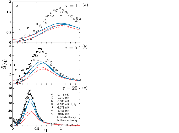
Figure 7: (a) Scaled structure factor ${\tilde{S}}(q)$ as a function of scaled wavevector $q$ at scaled time $\tau=1$; (b) the same for $\tau=5$; and (c) the same for $\tau=20$. The initial temperature for all quenches was $T_{c}\epsilon_{i}$= 10 mK. The symbols denote the experimental results of Bailey and Cannell as follows: $T_{c}\epsilon_{f}$ = $(\bigtriangleup)$ -0.116 mK, $(\bigcirc)$ -0.210 mK, $(\Box)$ -0.538 mK, $(\times)$ -1.036 mK, $(\bullet)$ -2.079 mK, $(\bigtriangledown)$ -5.156 mK, and $(\diamond)$ -10.37 mK. The blue solid and red dashed curves denote results of the adiabatic and isothermal theories, respectively. For the isothermal runs for each time, the upper curve denotes results for the deepest quench shown in that time frame, while the lower one is for the shallowest. This meaning also holds for the adiabatic runs in (a) and (b), but the reverse is true for (c).

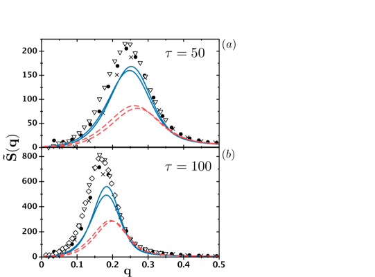
Figure 8: (a) Scaled structure factor ${\tilde{S}}(q)$ as a function of scaled wavevector $q$ at scaled time $\tau=50$; and (b) the same for $\tau=100$. The meaning of the symbols, curves and conditions are the same as in Fig.7(c).

As stated above, the experimental quenches of BC were for on-critical mixtures so $x_{0}=0$. To compare the adiabatic theory with these quenches, the thermodynamic quantities $T_{c},dT_{c}/dP,\rho_{c},\alpha_{P}$ and $C_{P}$ are needed. All can be found using Tables 1 and 2. Also needed are the two-phase values for $\xi_{0}$ and $\eta_{s}$. The former can be deduced from data in the same tables to be $\xi_{0}^{-}=1.13\AA$.

As mentioned above, the hydrodynamic shear viscosity, $\eta_{s}$, is not constant but is a singular function of $\epsilon$. In addition, the two-phase value of $\eta_{s}$ has not been determined, and at present there is no definite relation between the one and two-phase amplitudes. However, since the scaling form for $\eta_{s}$ is so weakly singular and the quenches are expected to be fast, $\eta_{s}$ was simply set equal to its one-phase value at $\xi=\xi_{f}$, i.e., $\eta_{s}\simeq{\bar{\eta}}(Q_{0}\xi_{f})^{z_{\eta}}$, where $\bar{\eta}$, $Q_{0}$ and $z_{\eta}$ are given in Table 1.

For each quench, the initial temperature, $\epsilon_{i}$, and the pressure change, $\Delta P$, are known. In the constant entropy approximation of the theory here, the final temperature, $\epsilon_{f}$, was determined by just integrating Eq. (II.35). Re-evaluation of the critical properties of 3MP+NE by BC allows us to ignore any uncertainty in $\epsilon_{f}$. The experimental intensity data was scaled by BCBailey (1993).

In Figures 7 and 8, the scaled structure factor ${\tilde{S}}(q)$ is shown as a function of the scaled wavevector $q$ for various scaled times $\tau$. The quenches shown all begin at $T_{c}\epsilon_{i}\approx 10$ mK and have final temperatures that range from $T_{c}\epsilon_{f}=-0.116$ mK to $-10.37$ mK. The solid and dashed curves denote results for the adiabatic and isothermal theories, respectively, while the points represent data of BC. For the isothermal runs for each time, the uppermost curve denotes the result for the deepest quench shown and the lower one denotes the shallowest. This meaning also holds for the adiabatics runs for $\tau=1$ and $5$, shown in Figures 7(a) and 7(b), but the reverse becomes true for larger times. The effect of a finite quench time is included in these results; the scaled quench time $\tau_{quench}$ ranged from $2\times 10^{-3}$ for the shallowest quench to $11$ for the deepest.

At a very early time, $\tau=1$, the prediction of the adiabatic theory for the peak height ${\tilde{S}}(q_{m})$ lags behind the data by a factor of 2. However, at later times, $\tau=20$ and $50$, the agreement with experiment is very good, within $20\%$. At the largest time for which data is available, $\tau=100$, the adiabatic theory appears to start lagging behind the data again, with the difference being $30\%$. On the other hand, the predictions of the adiabatic theory for the peak wavevector $q_{m}$ are within a few percent of the data at all times.

The LBM and thus KO theories are expected to work best at early times. For example, Mainville et al. obtained good agreement throughout the early stage, albeit with some fitting, between their experimental scattering data and the LBM theory.Mainville et al. (1997) Therefore, the disagreement between the adiabatic theory and experiment for the peak height ${\tilde{S}}(q_{m})$ at very early times is perplexing. One possibility is that setting the cut-off to a finite value removes the relaxation of high wavevector modes, $q>\alpha^{\ast}$, right after the quench. The relaxation of these modes then couple to lower $q$ ones, increasing their relaxation, like a wave moving through $q$-space. To examine this hypothesis, the cut-off of the theory was varied from $\alpha^{\ast}=1$ to $\alpha^{\ast}=\pi/2$. It was found that ${\tilde{S}}(q_{m})$ at $\tau=1$ varied by only 9% and 3% for the adiabatic and isothermal theories, respectively, for this cut-off range.

Another possible explanation is that the adiabatic theory has underestimated the temperature undershoot. Though whatever the cause, further research is needed.

The disagreement between theory and experiment at late times, is that at $\tau=50$, $q_{m}\simeq 0.2$, which, as has been discussed above, appears to be where the KO theory begins to break down. The isothermal theory predicts a peak height and peak wavevector that lags behind experiment at all times, the difference in ${\tilde{S}}(q_{m})$ becoming over a factor of three at the latest times.

Note that the theory results shown in Figures 7 and 8 are not quite the same as those in a previous report of the adiabatic theory, Ref.Donley and Langer (1993). One reason is that in Ref.Donley and Langer (1993) the “double gaussian” approximation was used to solve for the time evolution of $\rho_{1}(y)$. As mentioned above, while this approximation is more computationally efficient than solving the full PDE for $\rho_{1}(y)$, Eq.(IV.6), it tends to overestimate the growth of ${\tilde{S}}(q)$ for times such that $q_{m}\geq 0.3$. Advances in computer power in the years since Ref.Donley and Langer (1993) was published have made this approximation unnecessary. A second reason is that the form for the scaled free energy density $\phi(x)$ was different in the previous work. This previous form was constructed to satisfy a constraint in the limit of the cut-off $\alpha^{\ast}\rightarrow 0$ (see Ref.Donley (1991) for a detailed description). It was subsequently concluded that the added complexity to $\phi(x)$ needed for this constraint outweighed any improved accuracy of the theory, and so here the standard “$\varphi^{4}$” form for $\phi(x)$ was used instead.

As mentioned above, the isothermal theory predicts that if the fluid is in the critical region, the experimental data is scaled properly, and the scaled initial conditions and quench times are the same, then the scaled time evolution of any experimental run should be identical. It is interesting then whether the experimental data of BC show any violation of this scaling. Consider two experimental runs of BC with final temperatures $T_{c}\epsilon_{f}=-2.079$ mK and -0.202 mK.Bailey (1993) The initial temperatures were both at $\epsilon_{i}\simeq 5{|\epsilon_{f}|}$ to eliminate the effect of initial conditions. At $\tau=10$, ${\tilde{S}}(q_{m})$ was measured to be 16.6 and 18.8 for the first (-2.079 mK) and second (-0.202 mK) quench, respectively. The adiabatic theory predicts that ${\tilde{S}}(q_{m})=11.4$ and 12.3, for the first and second quench, respectively, while the isothermal theory predicts that ${\tilde{S}}(q_{m})=7.6$ and 7.7 for those quenches. Both the adiabatic and isothermal theories predict that $q_{m}\approx 0.47$ in agreement with both experimental runs. While the experimental violation of scaling is not large, the difference in ${\tilde{S}}(q_{m})$ for the two runs being 12%, the trend is in agreement with the adiabatic theory, which predicts a difference of 8%. So though there is certainly scatter in the data, this agreement at the least is suggestive that the temperature change during decomposition is appreciable for this fluid.

VII Summary and Discussion

In summary, the KO-LBM theory of spinodal decomposition in binary fluids was generalized to model experimental scenarios in which the fluid is quenched by changing the pressure and the subsequent phase separation occurs adiabatically.

The central idea of the approach here is that the coarse-grained free energy, ${\cal F}$, which governs the time evolution of the slowest modes, is constructed in a manner that creates a natural split in the degrees of freedom of the system. Those fast degrees of freedom that have been integrated out contribute to ${\cal F}$, but also to a free energy, $F_{r}$, that is independent of the configuration of the slow modes. It was shown that the fast degrees of freedom, through $F_{r}$, are able to act as a thermal reservoir for the slow modes. Any global constraint though, such as constant energy or entropy, indirectly relates the state of the reservoir, and thus its temperature, to the particular state of the slow modes. However, it was argued that these states need be related only in an average sense. With that approximation, an equation of motion for the average reservoir temperature was derived, it playing the same role as the assumed constant global system temperature in previous isothermal theories of decomposition.

In other words, if in a system there exists degrees of freedom that are able to sample their accessible states on timescales smaller than the characteristic change of the slower degrees of freedom, then these fast degrees of freedom can act as a reservoir to the slow ones. This model of nonequilibrium processes has become a common one.Kurchan (2005); Mosgaard et al. (2013); Bouchbinder and Langer (2013)

The extension of the isothermal theories of KO and LBM to adiabatic conditions then consisted of: this equation of motion for the reservoir temperature; estimates for various reservoir thermodynamic derivatives, such as the heat capacity, which appear in the temperature equation; and a specification of a temperature dependent coarse-grained free energy.

This “adiabatic” theory was then applied to an on-critical mixture of 3MP+NE. It was shown that the temperature change during decomposition is appreciable and accelerates the coarsening. The adiabatic and previous isothermal theories were then compared quantitatively, with no adjustable parameters, with data of Bailey and Cannell on 3MP+NE for the structure factor at various times during the early stage of decomposition. It was shown that there is a definite lack of agreement between the data and previous theory for the structure factor peak height, and that the adiabatic theory accounts for a substantial amount of this difference. The adiabatic theory also improves the agreement with experiment for the wavevector, $q_{m}$, of the structure factor peak. Differences between theory and experiment though indicate that the adiabatic theory may still be underestimating the effects of temperature changes during decomposition for 3MP+NE. Further research is needed to determine the cause.

The large temperature change during decomposition predicted for 3MP+NE is due partly to the size of the singular term in the isobaric heat capacity compared to the background term (see Table 1). Another binary fluid, isobutyric acid and water, has a much smaller singular term, and for it, at the same reduced temperatures as the Bailey and Cannell experiments, the predictions of the adiabatic and isothermal decomposition theories are essentially the same.Donley (1991) It is possible though that there are other binary fluids with even larger relative singular contributions to their heat capacity than 3MP+NE, making the adiabatic effect even more pronounced.

The adiabatic theory could possibly be extended to temperatures outside the critical region, e.g., for mixtures with longer range interactions such as polymers. However, if 3-D Ising critical scaling no longer holds, the isothermal KO/LBM theory itself becomes temperature dependent through at least the parameter $f_{1}$ (see Sec. II.2). So it is unclear how the predictions of this extended adiabatic theory would differ from the near-critical one developed here, especially as thermodynamic quantities such as the heat capacity are system dependent.

The behavior of the isothermal KO theory at later times was also analyzed. It was found for times $10^{2}<\tau\leq 10^{4}$, that $q_{m}$ scaled as $\tau^{-a_{q}}$, with $a_{q}\approx 0.46$.

While off-critical quenches were not examined here, it is expected that the adiabatic effect to be less for them since the heat released during phase separation should be largest for an on-critical mixture, it being roughly proportional to $1-x_{0}^{2}$, using Eq. (II.44).

Interestingly, it was shown in Section II.1.2 that the entropy increase during this adiabatic decomposition is well approximated as zero. That is, in the model here, the temperature rise from phase separation exactly compensates for the temperature undershoot caused by the incomplete relaxation of the slow modes during the quench, so that the final temperature reached is as if the whole process had been reversible. In that manner, if a fluid were quenched, allowed to phase separate at least partially, and then the pressure were reversed, the fluid upon re-mixing should reach a temperature very near its initial value. A similar two-step experiment was done by Siebert and Knobler in their study of nucleation.Onuki (2002); Siebert and Knobler (1984) While the arguments leading to this prediction of a (almost) constant entropy decomposition relied partly on the system being a near-critical binary fluid, it might be more general. Answers are left to future research.

*

Appendix A Coarse-grained energy

In this appendix it is shown that in the critical region, the dominant contribution to the average coarse-grained energy, ${\langle{\cal E}[c,{\bf v}]\rangle}$, comes from the heat of mixing. First, except when stated otherwise, all quantities are evaluated on-coexistence at the final equilibrium temperature, $T_{f}$, with a reduced cut-off $\alpha^{*}=1$. Now, using results of section II.2, ${\langle{\cal E}[c,{\bf v}]\rangle}$ is the sum of three terms: the gradient energy,

$$\langle{\cal E}_{K}\rangle= {KV\over 2}\Bigl{\langle}(\nabla c({\bf r}))^{2}\Bigr{\rangle}$$ (A.1)

$$= {KV\over 4\pi^{2}}\int_{0}^{\Lambda}dkk^{4}{\hat{S}}(k)$$

$$\simeq 0.003\biggl{(}{k_{B}T_{f}V\over\xi_{f}^{3}}\biggr{)},$$

the heat of mixing,

$$\langle{\cal E}_{mix}\rangle= -V\Bigl{\langle}T^{2}{\partial(f(c)/T)\over\partial T}\Bigr{\rangle}$$ (A.2)

$$= -\bigl{[}(\lambda_{2}-\lambda_{0}){1\over{|\epsilon_{f}|}}+\lambda_{0}\bigr{]}f_{1}\langle x^{2}\rangle{k_{B}T_{f}V\over\xi_{f}^{3}}$$

$$\simeq -{0.08\over{|\epsilon_{f}|}}\biggl{(}{k_{B}T_{f}V\over\xi_{f}^{3}}\biggr{)},$$

and the fluid kinetic energy,

$$\langle{\cal E}_{\bf v}\rangle= \ {1\over 2}\rho V\langle{\bf v}({\bf r})^{2}\rangle$$ (A.3)

$$\approx \ {1\over 2}\rho KV\int^{\Lambda}{d{\bf k}_{1}\over(2\pi)^{3}}{1\over\eta_{s}k_{1}^{2}}\int^{\Lambda}{d{\bf k}_{2}\over(2\pi)^{3}}{\bf k}_{2}\cdot{\bf\hat{T}}({\bf k}_{1})\cdot{{\bf k}_{2}}$$

$$\times \bigl{[}k_{2}^{2}-({\bf k}_{1}-{\bf k}_{2})^{2}\bigr{]}\bigl{[}Kk_{2}^{2}+A(t)\bigr{]}{\hat{S}}(|{\bf k}_{1}-{\bf k}_{2}|){\hat{S}}(k_{2})$$

$$= \ \biggl{(}{k_{B}T_{f}V\over\xi_{f}^{3}}\biggr{)}\Omega I_{{\bf v}}$$

Here, $I_{{\bf v}}$ is a scaled integral and $\Omega\equiv{\rho k_{B}T/(\eta_{s}^{2}\xi)}$ is a dimensionless number. To evaluate Eq.(A), the same overdamped approximation for ${\bf v}$ done in the KO theory was used, except that the noise term was dropped as it gives a term that is constant in the critical region. So, ${\bf v}\approx{\bf T}\cdot(\mu\nabla c)$. Similarly, four-point averages arising in Eq.(A) were evaluated in the manner done by KO for the equation of motion of ${\hat{S}}(k,t)$, Eq.(III.11).

The quenches for BC had final temperatures, ${|\epsilon_{f}|}\sim 10^{-5}$. Then, $\Omega\approx 10^{-5}$. The scaled integral $I_{{\bf v}}$ was zero in equilibrium. Out of equilibrium during a typical quench it was non-zero, but remained very small, $\sim 10^{-6}$. So, $\langle{\cal E}_{K}\rangle/\langle{\cal E}_{mix}\rangle\sim 10^{-6}$ and $\langle{\cal E}_{\bf v}\rangle/\langle{\cal E}_{mix}\rangle\leq 10^{-15}$, and so only $\langle{\cal E}_{mix}\rangle$ need be considered. It is interesting that while advection dominates the kinetics of unmixing, in the critical region its contribution to the energetics is negligible.

References

- Cahn (1968) J. W. Cahn, Trans. Metall. Soc. AIME 242, 166 (1968).
- Bray (1994) A. J. Bray, Adv. Phys. 43, 357 (1994).
- Onuki (2002) A. Onuki, Phase Transition Dynamics (Cambridge University Press, Cambridge, UK, 2002).
- Desai and Kapral (2009) R. C. Desai and R. Kapral, Dynamics of Self-Organized and Self-Assembled Structures (Cambridge University Press, Cambridge, UK, 2009).
- Boyanovsky et al. (2006) D. Boyanovsky, H. J. de Vega, and D. J. Schwarz, Annu. Rev. Nucl. Part. Sci. 56, 441 (2006).
- Cook (1970) H. E. Cook, Acta Metall. 18, 297 (1970).
- Langer et al. (1975) J. S. Langer, M. Bar-on, and H. D. Miller, Phys. Rev. A 11, 1417 (1975).
- N. G. Van Kampen (2007) N. G. Van Kampen, Stochastic Processes in Physics and Chemistry (North-Holland, Amsterdam, NLD, 2007).
- Yamada et al. (2019) R. Yamada, M. R. von Spakovsky, and W. T. Reynolds, Phys. Rev. E 99, 052121 (2019).
- Mainville et al. (1997) J. Mainville, Y. S. Yang, K. R. Elder, M. Sutton, K. F. Ludwig, and G. B. Stephenson, Phys. Rev. Lett. 78, 2787 (1997).
- Chou and Goldburg (1979) Y. C. Chou and W. I. Goldburg, Phys. Rev. A 20, 2105 (1979).
- Wong and Knobler (1978) N.-C. Wong and C. M. Knobler, J. Chem. Phys. 69, 725 (1978).
- Kawasaki and Ohta (1978) K. Kawasaki and T. Ohta, Prog. Theor. Phys. 59, 362 (1978).
- Bailey and Cannell (1993) A. E. Bailey and D. S. Cannell, Phys. Rev. Lett. 70, 2110 (1993).
- Bailey (1993) A. E. Bailey, PhD dissertation, University of California, Santa Barbara, Dept. of Physics (1993).
- Note (1) The exponent arises from the temperature dependence of the shear viscosity. See Table 1.
- Schmelzer and Ulbricht (1989) J. Schmelzer and H. Ulbricht, J. Colloid Interf. Sci. 128, 104 (1989).
- Onuki (1996) A. Onuki, Physica A 234, 189 (1996).
- Schmelzer and Milchev (1991) J. Schmelzer and A. Milchev, Phys. Lett. A 158, 307 (1991).
- Milchev et al. (1994) A. Milchev, I. Gerroff, and J. Schmelzer, Z. Phys. B 94, 101 (1994).
- Lebedev and Galenko (2019) V. G. Lebedev and P. K. Galenko, J. Expt. Theor. Phys. 129, 86 (2019).
- Mosgaard et al. (2013) L. D. Mosgaard, A. D. Jackson, and T. Heimburg, J. Chem. Phys. 139, 125101 (2013).
- Thoke et al. (2018) H. S. Thoke, L. F. Olsen, L. Dueland, R. P. Stock, T. Heimburg, and L. A. Bagatolli, J. Biol. Phys. 44, 419 (2018).
- Donley and Langer (1993) J. P. Donley and J. S. Langer, Phys. Rev. Lett. 71, 1573 (1993).
- Clerke et al. (1983) E. A. Clerke, J. V. Sengers, R. A. Ferrell, and J. K. Bhattacharjee, Phys. Rev. A 27, 2140 (1983).
- Greer and Hocken (1973) S. C. Greer and R. Hocken, J. Chem. Phys. 63, 5067 (1973).
- Sorensen (1982) C. M. Sorensen, Int. J. Thermophys. 3, 365 (1982).
- Burstyn et al. (1983) H. C. Burstyn, J. V. Sengers, J. K. Bhattacharjee, and R. A. Ferrell, Phys. Rev. A 28, 1567 (1983).
- Tanaka and Wada (1983) H. Tanaka and Y. Wada, Chem. Phys. 78, 143 (1983).
- Fisher and Chen (1985) M. E. Fisher and J.-H. Chen, J. Physique (Paris) 46, 1645 (1985).
- Liu and Fisher (1989) A. J. Liu and M. E. Fisher, Physica A 156, 35 (1989).