Well-posedness and Robust Preconditioners
for the Discretized Fluid-Structure Interaction Systems

Abstract

In this paper we develop a family of preconditioners for the linear algebraic systems arising from the arbitrary Lagrangian-Eulerian discretization of some fluid-structure interaction models. After the time discretization, we formulate the fluid-structure interaction equations as saddle point problems and prove the uniform well-posedness. Then we discretize the space dimension by finite element methods and prove their uniform well-posedness by two different approaches under appropriate assumptions. The uniform well-posedness makes it possible to design robust preconditioners for the discretized fluid-structure interaction systems. Numerical examples are presented to show the robustness and efficiency of these preconditioners.

Keywords: fluid-structure interaction, stabilization, robust preconditioners

1 Introduction

Fluid-structure interaction (FSI) is a much studied topic aimed at understanding the interaction between some moving structure and fluid and how their interaction affects the interface between them. FSI has a wide range of applications in many areas including hemodynamics [26, 43, 44, 18] and wind/hydro turbines [8, 32, 7, 6].

FSI problems are computationally challenging. The computational domain of FSI consists of fluid and structure subdomains. The position of the interface between fluid domain and structure domain is time dependent. Therefore, the shape of the fluid domain is one of the unknowns, increasing the nonlinearity of the FSI problems.

Many numerical approaches have been proposed to tackle the interface problem of FSI. The arbitrary Lagrangian-Eulerian (ALE) method is commonly used. ALE adapts the fluid mesh to match the displacement of structure on interface. Other approaches, such as the fictitious domain method [29, 53] and the immersed boundary method [54, 49, 41], have inconsistent fluid and structure meshes and, therefore, need special treatment at the interface, such as interpolation between different meshes. In this paper, we focus on the ALE method.

There is much research focused solving fluid-structure interaction problem numerically using ALE formulation. These studies can be roughly classified into partitioned approaches and monolithic approaches [22]. Partitioned approaches employ single-physics solvers to solve the fluid and structure problems separately and then couple them by the interface conditions. Monolithic approaches solve the fluid and structure problems simultaneously. Depending on whether the interface conditions are exactly enforced at every time step, these approaches can also be classified into weakly and strongly coupled algorithms. Weakly coupled partitioned approaches are usually considered unstable due to the added-mass effect [15]. A semi-implicit approach proposed in [23] can avoid the added-mass effect for a wide range of applications, but it is subject to pressure boundary conditions. Several types of semi-implicit methods were proposed in [42, 37]. Strongly coupled approaches are preferred for their stability. Although it is possible to achieve the strong coupling via partitioned solvers (by fixed-point iteration, for example), they usually introduce prohibitive computational costs due to slow convergence [25]. In this paper we consider strongly coupled monolithic approaches and address some solver issues. Monolithic approaches give us larger linear systems, for which efficient solvers are needed.

A great deal of work has been carried out to develop monolithic solvers for FSI [27, 47, 14, 5]. In [30], a fully-coupled solution strategy is proposed to solve the FSI problem with large structure displacement. The nonlinearity is handled by Newton’s method and various approaches to solve the Jacobian system are proposed. Block triangular preconditioners and pressure Schur complement preconditioners are used for the preconditioned Krylov subspace solvers. However, in [27] it is pointed out that block preconditioning for fluid and structure separately cannot resolve the coupling between fields and it is proposed that structure degrees of freedoms on interface be eliminated in order to effectively precondition degrees of freedom at the interface. In [5, 3, 4], a Newton-Krylov-Schwarz method for FSI is developed. Additive Schwarz preconditioners are used for Krylov subspace solvers and two-level methods are also developed. In [1, 2], ILU preconditioners and inexact block-LU preconditioners are proposed to solve FSI problems.

In this paper, we reformulate semi-discretized systems of FSI as saddle point problems with fluid velocity, pressure and structure velocity as unknowns. The ALE mapping is decoupled from the solution of the velocity and pressure. Then, we carry out our theoretical analysis and solver design under this framework. With particular choice of norms, we prove that the saddle point problem is well-posed.

For the finite element discretization of FSI, we propose two approaches to prove the well-posedness. The first introduces a stabilization term to the fluid equations and the second adopts a norm of the velocity space that depends on the choice of the pressure space. Both of these approaches lead to uniform well-posedness of the finite element discretization of the FSI model under appropriate assumptions.

Based on the uniform well-posedness, we propose optimal preconditioners based on the framework in [36, 55] such that the preconditioned linear systems have uniformly bounded condition numbers. Then, we compare the proposed preconditioners with the augmented Lagrangian preconditioners [11, 9, 10, 40]. To test the preconditioners, we solve the linear systems coming from the discretization of the Turek and Hron benchmark problems [48]. The iteration counts of GMRes with several preconditioners are compared.

The rest of this paper is organized as follows. In section 2, we introduce an FSI model and the ALE method. In section 3, we study the proposed time and space discretization and its well-posedness. In section 4, we propose optimal preconditioners for the discretized systems and demonstrate their performance with numerical examples.

2 An FSI model

We consider a domain $\Omega\subset\mathbb{R}^{N}(N=2,3)$ with a fluid occupying the upper half $\Omega_{f}$ and a solid occupying the lower half $\Omega_{s}$, as illustrated in Figure 1.

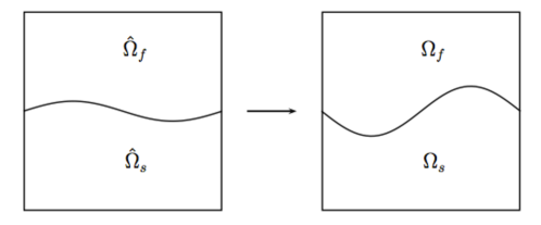
Figure 1: Moving domains of FSI

Let $\Gamma:=\partial\Omega_{f}\cap\partial\Omega_{s}$ be the interface of the fluid domain and the solid domain. On the outer boundary of the solid $\partial\Omega_{s}\backslash\Gamma$, the solid is clamped; namely, the displacement of the solid is zero on $\partial\Omega_{s}\backslash\Gamma$. In this paper, we always assume that both $\partial\Omega_{s}\backslash\Gamma$ and $\partial\Omega_{f}\backslash\Gamma$ have positive measures.

In addition, we assume that the interaction of the fluid and solid only occurs at the interface, and the interface $\Gamma$ may move over time due to this interaction. We assume that the outer boundary is fixed. In the dynamic setting, we use $\Omega_{f}(t)$ and $\Omega_{s}(t)$ to denote the domains at time $t\in[0,T]$. The domains satisfy $\bar{\Omega}=\bar{\Omega}_{f}(t)\cup\bar{\Omega}_{s}(t)$ and $\Gamma(t)=\partial\Omega_{f}(t)\cap\partial\Omega_{s}(t)$.

We denote the reference domains by

$$\hat{\Omega}_{f}=\Omega_{f}(0),\quad\hat{\Omega}_{s}=\Omega_{s}(0)$$

and the domains at time $t$ by

$$\Omega_{f}=\Omega_{f}(t),\quad\Omega_{s}=\Omega_{s}(t).$$

The motion in the fluid and structure can be characterized by a flow map $\mathbf{x}(\hat{\mathbf{x}},t)$; namely, the position of the particle $\hat{\mathbf{x}}$ at time $t$ is $\mathbf{x}(\hat{\mathbf{x}},t)$. Then, given $t>0$, $\mathbf{x}(\cdot,t)$ is a diffeomorphism from $\Omega(0)$ to $\Omega(t)$.

For $({\hat{\mathbf{x}}},t)\in\Omega(0)\times[0,T]$, we introduce the following variables in Lagrangian coordinates : the displacement $\hat{\mathbf{u}}({{\hat{\mathbf{x}}}},t)={\mathbf{x}}({\hat{\mathbf{x}}},t)-{\hat{\mathbf{x}}}$, the velocity $\displaystyle\hat{\mathbf{v}}({\hat{\mathbf{x}}},t)=\frac{\partial\hat{\mathbf{x}}}{\partial t}$, the deformation tensor $\displaystyle{F}({\hat{\mathbf{x}}},t)=\frac{\partial{\mathbf{x}}}{\partial{\hat{\mathbf{x}}}}({\hat{\mathbf{x}}},t)$, and its determinant $\displaystyle{J}({\hat{\mathbf{x}}},t)=det({F}({\hat{\mathbf{x}}},t))$. Using the relationship $\mathbf{x}=\mathbf{x}(\hat{\mathbf{x}},t)$, we also introduce the velocity in Eulerian coordinates: ${\mathbf{v}}({\mathbf{x}},t)=\hat{\mathbf{v}}({\hat{\mathbf{x}}},t)$. The symmetric part of the gradient is denoted by $\displaystyle\boldsymbol{\epsilon}(\mathbf{v})=\frac{\nabla\mathbf{v}+(\nabla\mathbf{v})^{T}}{2}.$

Let us now introduce a simple FSI model which consists of the incompressible Navier-Stokes equations for the fluid (in Eulerian coordinates) and linear elasticity equations for the structure (in Lagrangian coordinates).

For clarity, we start with the momentum equations for fluid and solid both in Eulerian coordinates:

$$\rho_{f}D_{t}\mathbf{v}_{f}-\nabla\cdot\boldsymbol{\sigma}_{f}=g_{f},\quad\mbox{in }\Omega_{f},$$

and

$$\rho_{s}D_{t}\mathbf{v}_{s}-\nabla\cdot\boldsymbol{\sigma}_{s}=g_{s},\quad\mbox{in }\Omega_{s}.$$

Here $\boldsymbol{\sigma}_{f}$ and $\boldsymbol{\sigma}_{s}$ are the Cauchy stress tensors for fluid and structure, respectively. Here $D_{t}\mathbf{v}_{f}$ and $D_{t}\mathbf{v}_{s}$ are the material derivatives.

On the interface $\Gamma=\partial\Omega_{f}\cap\partial\Omega_{s}$, the interface conditions are given in Eulerian coordinates as

$$\mathbf{v}_{f}=\mathbf{v}_{s}\quad\mbox{and}\quad\boldsymbol{\sigma}_{f}\mathbf{n}=\boldsymbol{\sigma}_{s}\mathbf{n}\quad\mbox{ on }\Gamma.$$ (1)

Note that we neglect some effects such as the surface tension in this model and thus the stress is continuous on interface.

While we keep the Eulerian description for the fluid model, we use the Lagrangian description for the structure. Accordingly, we introduce the following Sobolev spaces:

$$\mathbb{V}:=\{(\mathbf{v}_{f},\hat{\mathbf{v}}_{s})\in H^{1}_{D}(\Omega_{f}(t))\times H^{1}_{D}(\hat{\Omega}_{s})\text{ such that }\mathbf{v}_{f}\circ\mathbf{x}_{s}=\hat{\mathbf{v}}_{s},\text{ on }\hat{\Gamma}\},$$ (2)

where

$$H^{1}_{D}(\Omega_{f}(t)):=\{\mathbf{u}\in(H^{1}(\Omega_{f}(t)))^{N}|\mathbf{u}=0,\text{ on }\partial\Omega\cap\partial\Omega_{f}\},$$

$$H^{1}_{D}(\hat{\Omega}_{s}):=\{\mathbf{u}\in(H^{1}(\hat{\Omega}_{s}))^{N}|\mathbf{u}=0,\text{ on }\partial\Omega\cap\partial\hat{\Omega}_{s}\},$$

and

$$\mathbb{Q}:=L^{2}(\Omega_{f}(t)).$$

$\mathbb{V}$ is defined for the fluid velocity in Eulerian coordinates and the structure velocity in Lagrangian coordinates. The condition $\mathbf{v}_{f}\circ\mathbf{x}_{s}=\hat{\mathbf{v}}_{s}$ is used to enforce continuity of velocity in (1). We will discuss the choice of norms for these spaces in the next section.

In order to formulate the problem weakly, we use test functions defined on $\Omega$, With the test function $\boldsymbol{\phi}\in H_{0}^{1}(\Omega)$, we first write the weak form for the fluid and structure, respectively:

$$\int_{\Omega_{f}}\rho_{f}D_{t}\mathbf{v}_{f}\boldsymbol{\phi}d\mathbf{x}+\int_{\Omega_{f}}\boldsymbol{\sigma}_{f}:\boldsymbol{\epsilon}(\boldsymbol{\phi})d\mathbf{x}-\int_{\Gamma}\boldsymbol{\sigma}_{f}\mathbf{n}_{f}\cdot\boldsymbol{\phi}d\mathbf{x}=\int_{\Omega_{f}}g_{f}\boldsymbol{\phi}d\mathbf{x},$$

$$\int_{\Omega_{s}}\rho_{s}D_{t}\mathbf{v}_{s}\boldsymbol{\phi}d\mathbf{x}+\int_{\Omega_{s}}\boldsymbol{\sigma}_{s}:\boldsymbol{\epsilon}(\boldsymbol{\phi})d\mathbf{x}-\int_{\Gamma}\boldsymbol{\sigma}_{s}\mathbf{n}_{s}\cdot\boldsymbol{\phi}d\mathbf{x}=\int_{\Omega_{s}}g_{s}\boldsymbol{\phi}d\mathbf{x}.$$

We add these two equations based on interface conditions (1):

$$\int_{\Omega_{f}}\rho_{f}D_{t}\mathbf{v}_{f}\boldsymbol{\phi}d\mathbf{x}+\int_{\Omega_{f}}\boldsymbol{\sigma}_{f}:\boldsymbol{\epsilon}(\boldsymbol{\phi})d\mathbf{x}+\int_{\Omega_{s}}\rho_{s}D_{t}\mathbf{v}_{s}\boldsymbol{\phi}d\mathbf{x} +\int_{\Omega_{s}}\boldsymbol{\sigma}_{s}:\boldsymbol{\epsilon}(\boldsymbol{\phi})d\mathbf{x}$$

$$= \int_{\Omega_{f}}g_{f}\boldsymbol{\phi}d\mathbf{x}+\int_{\Omega_{s}}g_{s}\boldsymbol{\phi}d\mathbf{x}.$$

By a change of coordinates $\mathbf{x}=\mathbf{x}(\hat{\mathbf{x}},t),$ the stress term of structure part can be written in Lagrangian coordinates

$$\int_{\Omega_{s}}\boldsymbol{\sigma}_{s}:\boldsymbol{\epsilon}(\boldsymbol{\phi})d\mathbf{x}=\int_{\hat{\Omega}_{s}}\hat{\boldsymbol{\sigma}}_{s}:\nabla_{\hat{\mathbf{x}}}\hat{\boldsymbol{\phi}}F^{-1}\hat{J}d\hat{\mathbf{x}}=\int_{\hat{\Omega}_{s}}(J\hat{\boldsymbol{\sigma}}_{s}F^{-T}):\nabla_{\hat{\mathbf{x}}}\hat{\boldsymbol{\phi}}d\hat{\mathbf{x}},$$

where $\hat{\boldsymbol{\phi}}(\hat{\mathbf{x}},t)=\boldsymbol{\phi}(\mathbf{x}(\hat{\mathbf{x}},t),t)$ and $\hat{\boldsymbol{\sigma}}_{s}(\hat{\mathbf{x}},t)=\boldsymbol{\sigma}_{s}(\mathbf{x}(\hat{\mathbf{x}},t),t)$. We also change the coordinates for the inertial term and the body force term. Then, we get the following weak form of FSI

$$\int_{\Omega_{f}}\rho_{f}D_{t}\mathbf{v}_{f}\boldsymbol{\phi}+\boldsymbol{\sigma}_{f}:\boldsymbol{\epsilon}(\boldsymbol{\phi})d\mathbf{x}+\int_{\hat{\Omega}_{s}}\hat{\rho}_{s}\partial_{tt}\hat{\mathbf{u}}_{s}\hat{\boldsymbol{\phi}}+ \mathbf{P}_{s}:\nabla\hat{\boldsymbol{\phi}}d\hat{\mathbf{x}}$$ (3)

$$=\int_{\Omega_{f}}g_{f}\boldsymbol{\phi}d\mathbf{x}+\int_{\hat{\Omega}_{s}}J\hat{g}_{s}\boldsymbol{\phi}d\hat{\mathbf{x}},$$

which holds for any $\boldsymbol{\phi}\in\mathbb{V}$. Here, the density of the structure $\hat{\rho}_{s}$ is defined as

$$\hat{\rho}_{s}(\hat{\mathbf{x}},t)=J(\hat{\mathbf{x}},t)\rho_{s}(\mathbf{x}(\hat{\mathbf{x}},t),t)$$

and $\mathbf{P}_{s}=J\hat{\boldsymbol{\sigma}}_{s}F^{-T}$ is the first Piola-Kirchhoff stress. By the conservation of mass, $\hat{\rho}_{s}$ is independent of $t$.

The variational formulation (3) holds for general fluid and structure models described by the Cauchy stresses $\sigma_{f}$ and $\sigma_{s}$, respectively. We now make some specific choices for $\sigma_{f}$ and $\sigma_{s}$.

For the fluid, we use the incompressible Newtonian model, which is given by

$$\boldsymbol{\boldsymbol{\sigma}}_{f}=2\mu_{f}\boldsymbol{\epsilon}(\mathbf{v}_{f})-p\mathbf{I}$$ (4)

and

$$\nabla\cdot\mathbf{v}_{f}=0.$$

For the structure, we use the linear elasticity model (for small deformations) in Lagrangian coordinates, which corresponds to the following approximation:

$$\mathbf{P}_{s}\approx\tilde{\mathbf{P}}_{s}:=\mu_{s}\boldsymbol{\epsilon}(\hat{\mathbf{u}}_{s})+\lambda_{s}\nabla\cdot\hat{\mathbf{u}}_{s}\mathbf{I}.$$ (5)

Initial and boundary conditions

We consider the following Dirichlet boundary conditions

$$\mathbf{v}_{f} =\mathbf{v}_{f}^{D}, \partial\Omega_{f}\cap\partial\Omega,$$ on

$$\hat{\mathbf{u}}_{s} =0, \partial\Omega_{s}\cap\partial\Omega,$$ on

and initial conditions

$$\hat{\mathbf{u}}_{s}(0)=\mathbf{u}_{s,0},\quad\partial_{t}\hat{\mathbf{u}}_{s}(0) =\mathbf{u}_{s,1},\quad\mathbf{v}_{f}(0) =\mathbf{v}_{f,0}.$$

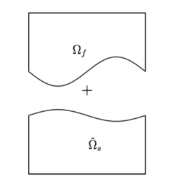
Figure 2: Computational domains of FSI

In the rest of this paper, we do not rewrite the initial conditions in the weak formulations for brevity. Moreover, we assume $\mathbf{v}_{f}^{D}=0$. That is, there are only homogeneous Dirichlet boundary conditions for the fluid problem.

Together with the continuity equation and interface condition, the weak formulation of FSI is as follows:

The weak formulation of FSI:

Find $\mathbf{v}_{f}$, $p$ and $\hat{\mathbf{u}}_{s}$ such that for any given $t>0$, the following equations hold for any $(\boldsymbol{\phi},\hat{\boldsymbol{\phi}})\in\mathbb{V}$ and $q\in\mathbb{Q}$

$$\left\{\begin{aligned} (\hat{\rho}_{s}\partial_{tt}\hat{\mathbf{u}}_{s},\hat{\boldsymbol{\phi}})_{\hat{\Omega}_{s}}+\left(\rho_{f}D_{t}\mathbf{v}_{f},\boldsymbol{\phi}\right)_{\Omega_{f}}+(\tilde{\mathbf{P}}_{s},\nabla\hat{\boldsymbol{\phi}})_{\hat{\Omega}_{s}}&+(\boldsymbol{\sigma}_{f},\boldsymbol{\epsilon}(\boldsymbol{\phi}))_{\Omega_{f}}\\ &=\langle J\hat{g}_{s},\hat{\boldsymbol{\phi}}\rangle+\langle g_{f},\boldsymbol{\phi}\rangle,\\ (\nabla\cdot\mathbf{v}_{f},q)_{\Omega_{f}}&=0,\\ \mathbf{v}_{f}\circ\mathbf{x}_{s}&=\partial_{t}\hat{\mathbf{u}}_{s},\quad\text{on }\hat{\Gamma}.\\ \end{aligned}\right.$$ (6)

Remark.

The solution $\mathbf{v}_{f}$, $p$ and $\hat{\mathbf{u}}_{s}$ are in some specific function spaces that require sufficient regularity in the time variable. Since the regularity in time variable is not discussed in this paper, we do not introduce these spaces in the weak formulation.

3 Finite element discretization based on the ALE method

In this section, we consider both time and space discretizations of Equations (6) and discuss the well-posedness. We first discretize the time variable $t$ with uniform time step size $k=\Delta t$:

$$t^{n}=nk,\quad n=0,1,\ldots,$$

and use the finite difference method to discretize time derivatives. For the space-time formulation of FSI, we refer to [46, 45] and references therein.

Since the function spaces usually depend on $t$, we use the superscript $n$ to indicate that the function space is at time $t^{n}.$ For example,

$$\mathbb{V}^{n}:=\{(\mathbf{v}_{f},\hat{\mathbf{v}}_{s})\in H^{1}_{D}(\Omega_{f}(t^{n}))\times H^{1}_{D}(\hat{\Omega}_{s})\text{ such that }\mathbf{v}_{f}\circ\mathbf{x}_{s}^{n}=\hat{\mathbf{v}}_{s},\text{ on }\hat{\Gamma}\}.$$

We use an ALE approach for the discretization of spatial variable. In this approach, the structure domain is discretized by a fixed mesh on the initial domain $\hat{\Omega}_{s}$ and the fluid domain is discretized by a sequence of moving meshes on the moving domain $\Omega_{f}(t)$.

3.1 Time discretization

Time discretization for the structure domain

Without loss of generality, we consider for the time discretization of the structure variables the following simple finite difference schemes:

$$(\partial_{t}\hat{\mathbf{u}}_{s})^{n+1}\approx (\partial_{t,h}\hat{\mathbf{u}}_{s})^{n+1}\equiv\frac{\hat{\mathbf{u}}_{s}^{n+1}-\hat{\mathbf{u}}_{s}^{n}}{k},$$ (7)

$$(\partial_{tt}\hat{\mathbf{u}}_{s})^{n+1}\approx (\partial_{tt,h}\hat{\mathbf{u}}_{s})^{n+1}\equiv\frac{\hat{\mathbf{u}}_{s}^{n+1}-2\hat{\mathbf{u}}_{s}^{n}+\hat{\mathbf{u}}_{s}^{n-1}}{k^{2}}.$$

Other popular time discretization schemes such as the Newmark method [38] can also be used.

Time discretization for the fluid domain by moving meshes

We need to find a mapping to move the fluid mesh such that it matches the structure displacement on $\hat{\Gamma}$ and remains non-degenerate in $\Omega_{f}$ as time evolves. This mapping is a diffeomorphism in continuous case, and we use piecewise polynomials to approximate it in discrete case. For a triangular mesh, only piecewise linear functions preserve the triangular shape of the elements in the mesh. In the rest of this paper, we assume that the mesh motion is piecewise linear. We denote the image of $\hat{\Omega}_{f}$ under the piecewise linear map $\mathbf{x}_{h,f}$ by $\Omega_{f}^{n}$. $\Omega_{f}^{n}$ is discretized by a moving mesh with respect to time, denoted by $T_{h}(\Omega_{f}^{n})$. Note that $\Omega_{f}^{n}$ is a polygonal domain in 2D, and a polyhedral domain in 3D. $\Omega_{f}^{n}$ is a result of numerical discretization, and is, in general, different from the domain shape $\Omega_{f}(t^{n})$ in the analytic solution of $(\ref{eq:FSI_weak})$.

The technique we use to determine the mesh motion is the ALE method. First introduced for finite element discretizations of incompressible fluids in [33, 20], the ALE method provides an approach to finding the fluid mesh that can fit the moving domain $\Omega_{f}(t)$.

There are two main ingredients in the ALE approach:

1. Defining how the grid is moving with respect to time such that it matches the structure displacement at the fluid-structure interface.

2. Defining how the material derivatives are discretized on the moving grid.

Given the structure trajectory $\mathbf{x}_{s}^{n}$ defined on $\hat{\Gamma},$ the moving grid can be described by a diffeomorphism ${\mathcal{A}}^{n}:\hat{\Omega}_{f}\mapsto\Omega_{f}$ that satisfies

$$\left\{\begin{aligned} {\mathcal{A}}^{n}(\hat{\mathbf{x}})&=\hat{\mathbf{x}},&\text{ on }&\partial\hat{\Omega}_{f}\cap\partial\hat{\Omega},\\ {\mathcal{A}}^{n}(\hat{\mathbf{x}})&=\mathbf{x}_{s}^{n}(\hat{\mathbf{x}},t),&\text{ on }&\hat{\Gamma}.\\ \end{aligned}\right.$$ (8)

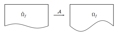
Figure 3: ALE mapping

ALE mappings satisfying (8) are by no means unique. In the interior of $\hat{\Omega}_{f}$, the ALE mapping can be “arbitrary”. One popular approach to uniquely determine ${\mathcal{A}}$ is to solve partial differential equations

$$\mathcal{L}{\mathcal{A}}=0,\quad\mbox{in }\hat{\Omega}_{f}.$$

A popular choice for the operator $\mathcal{L}$ is the Laplacian, $\mathcal{L}=-\Delta.$

To improve the quality of the fluid mesh with respect to the displacement of the structure near the interface, the following elasticity model is often used [21]

$$\mathcal{LA}=-\mu\Delta\mathcal{A}-\lambda\nabla(\nabla\cdot\mathcal{A}).$$

For more choices of formulating the ALE problem, we refer to [8, 20] and references therein.

Discretization of the material derivative

With the ALE mapping ${\mathcal{A}}$ introduced, material derivatives can be written as follows

$$D_{t}\mathbf{v} = \partial_{t}\mathbf{v}+(\mathbf{v}\cdot\nabla)\mathbf{v}$$

$$= \partial_{t}\mathbf{v}+(\partial_{t}{\mathcal{A}}\cdot\nabla)\mathbf{v}+((\mathbf{v}-\partial_{t}{\mathcal{A}})\cdot\nabla)\mathbf{v}$$

$$= \partial_{t}\mathbf{v}({\mathcal{A}}(\hat{\mathbf{x}},t),t))+((\mathbf{v}-\partial_{t}{\mathcal{A}})\cdot\nabla)\mathbf{v}.$$

Using the simple approximation:

$$\partial_{t}\mathbf{v}({\mathcal{A}}(\hat{\mathbf{x}},t^{n+1}),t^{n+1}))\approx\partial^{\mathcal{A}}_{t,h}\mathbf{v}|_{({\mathcal{A}}(\hat{\mathbf{x}},t^{n+1}),t^{n+1})}:=\frac{v({\mathcal{A}}(\hat{\mathbf{x}},t^{n+1}),t^{n+1})-v({\mathcal{A}}(\hat{\mathbf{x}},t^{n}),t^{n})}{k}$$

and

$$(\partial_{t}{\mathcal{A}})(\hat{\mathbf{x}},t)\approx(\partial_{t,h}{\mathcal{A}})(\hat{\mathbf{x}},t):=\frac{{\mathcal{A}}(\hat{\mathbf{x}},t^{n+1})-{\mathcal{A}}(\hat{\mathbf{x}},t^{n})}{k},$$

we obtain an approximation of material derivatives as follows:

$$(D_{t}\mathbf{v})^{n+1}\approx(D_{t,h}\mathbf{v})^{n+1}:=\partial^{\mathcal{A}}_{t,h}\mathbf{v}(\mathbf{x},t^{n+1})+((\mathbf{v}-\partial_{t,h}{\mathcal{A}})\cdot\nabla)\mathbf{v}(\mathbf{x},t^{n+1}),$$ (9)

for $\mathbf{x}={\mathcal{A}}(\hat{\mathbf{x}},t^{n+1})$.

With the aforementioned discretization of material derivatives, we write the momentum equation of Navier-Stokes equations as

$$\rho_{f}\partial^{\mathcal{A}}_{t,h}\mathbf{v}_{f}+\rho_{f}((\mathbf{v}_{f}-\partial_{t,h}{\mathcal{A}})\cdot\nabla)\mathbf{v}_{f}-\mu\nabla\cdot\boldsymbol{\sigma}_{f}=g_{f}.$$

Once the time derivatives are discretized using (7) and (9), we obtain the fully implicit scheme.

Fully implicit (FI) scheme:

find $\mathbf{v}^{n+1}_{f}\in\mathbb{V}_{f}^{n+1}$, $\hat{\mathbf{u}}^{n+1}_{s}\in\hat{\mathbb{V}}_{s}$, $p\in\mathbb{Q}^{n+1}$ and ${\mathcal{A}}^{n+1}\in H^{1}(\hat{\Omega}_{f})$ such that for any $(\boldsymbol{\phi},\hat{\boldsymbol{\phi}})\in\mathbb{V}^{n+1}$ and $q\in\mathbb{Q}^{n+1}$,

$$\left\{\begin{aligned} (\hat{\rho}_{s}(\partial_{tt,h}\hat{\mathbf{u}}_{s})^{n+1},\hat{\boldsymbol{\phi}})_{\hat{\Omega}_{s}}+(\rho_{f}(D_{t,h}\mathbf{v}_{f})^{n+1},&\boldsymbol{\phi})_{\Omega_{f}}+(\boldsymbol{\sigma}_{f}^{n+1},\boldsymbol{\epsilon}(\boldsymbol{\phi}))_{\Omega_{f}}\\ +(\tilde{\mathbf{P}}^{n+1}_{s},\nabla\hat{\boldsymbol{\phi}})_{\hat{\Omega}_{s}}&=\langle J\hat{g}_{s},\hat{\boldsymbol{\phi}}\rangle+\langle g_{f},\boldsymbol{\phi}\rangle,\\ (\nabla\cdot\mathbf{v}^{n+1}_{f},q)_{\Omega_{f}}&=0,\\ \mathbf{v}_{f}^{n+1}\circ{\mathbf{x}_{s}^{n+1}}&=(\partial_{t,h}\hat{\mathbf{u}}_{s})^{n+1},\quad\mbox{ on }\hat{\Gamma},\\ \mathcal{L}{\mathcal{A}}^{n+1}&=0,~{}~{}~{}~{}~{}~{}~{}~{}\qquad\text{ in }\hat{\Omega}_{f},\\ {\mathcal{A}}^{n+1}(\hat{\mathbf{x}})&=\hat{\mathbf{x}},~{}~{}~{}~{}~{}~{}~{}\qquad\text{ on }\partial\hat{\Omega}_{f}\cap\partial\hat{\Omega},\\ {\mathcal{A}}^{n+1}(\hat{\mathbf{x}})&=\hat{\mathbf{x}}+\hat{\mathbf{u}}_{s}^{n+1},~{}~{}~{}~{}\text{ on }\hat{\Gamma},\\ \end{aligned}\right.$$ (10)

The structure displacement $\hat{\mathbf{u}}_{s}^{n+1}$ serves as the boundary condition for the ALE problem. Note that ${\mathcal{A}}^{n+1}$ has to be a homeomorphism. The fluid stress $\boldsymbol{\sigma}_{f}^{n+1}$ is defined by (4) in terms of $\mathbf{v}_{f}^{n+1}$ and $p^{n+1}$. The structure stress $\tilde{\mathbf{P}}_{s}^{n+1}$ is defined by (5) in terms of $\hat{\mathbf{u}}_{s}^{n+1}$.

In the FI scheme, nonlinearity comes from the convection term and the dependence of the Navier-Stokes (NS) equations on the ALE mapping. To solve (10), Newton’s method or fixed-point iteration may be used to linearize the problem.

Another frequently used linearization of the FI scheme is the following geometry-convective explicit scheme[18, 17, 35]

Geometry-convective explicit (GCE) scheme:

Find $\mathbf{v}^{n+1}_{f}\in H_{D}^{1}(\Omega_{f}(t^{n}))$, $\hat{\mathbf{u}}^{n+1}_{s}\in H_{D}^{1}(\hat{\Omega}_{s})$, $p\in L^{2}(\Omega_{f}(t^{n}))$ and ${\mathcal{A}}^{n+1}\in H^{1}(\hat{\Omega}_{f})$ such that for any $(\boldsymbol{\phi},\hat{\boldsymbol{\phi}})\in\mathbb{V}^{n}$ and $q\in\mathbb{Q}^{n}$,

$$\footnotesize\left\{\begin{aligned} (\rho_{f}(\partial_{t,h}^{{\mathcal{A}}}\mathbf{v}_{f})^{n+1},\boldsymbol{\phi})_{\Omega_{f}}+(\hat{\rho}_{s}&(\partial_{tt,h}\hat{\mathbf{u}}_{s})^{n+1},\hat{\boldsymbol{\phi}})_{\hat{\Omega}_{s}}+(\boldsymbol{\sigma}_{f}^{n+1},\boldsymbol{\epsilon}(\boldsymbol{\phi}))_{\Omega_{f}}\\ +(\tilde{\mathbf{P}}_{s}^{n+1},\nabla(\hat{\boldsymbol{\phi}}))_{\hat{\Omega}_{s}}&=\langle g_{f}+((\mathbf{v}_{f}^{n}-\partial_{t,h}{\mathcal{A}}^{n+1})\cdot\nabla)\mathbf{v}_{f}^{n},\boldsymbol{\phi}\rangle_{\Omega_{f}}+\langle J\hat{g}_{s},\hat{\boldsymbol{\phi}}\rangle_{\hat{\Omega}_{s}},\\ (\nabla\cdot\mathbf{v}^{n+1}_{f},q)_{\Omega_{f}}&=0,\\ \mathbf{v}_{f}^{n+1}\circ{\mathbf{x}_{h}^{n}}&=(\partial_{t,h}\hat{\mathbf{u}}_{s})^{n+1},\quad\qquad\qquad\qquad\mbox{ on }\hat{\Gamma},\\ \mathcal{L}{\mathcal{A}}^{n+1}&=0,~{}~{}~{}~{}~{}~{}~{}~{}~{}~{}~{}\qquad\qquad\qquad\qquad\text{ in }\hat{\Omega}_{f},\\ {\mathcal{A}}^{n+1}(\hat{\mathbf{x}})&=\hat{\mathbf{x}},~{}~{}~{}~{}~{}~{}~{}~{}~{}~{}~{}\qquad\qquad\qquad\qquad\text{ on }\partial\hat{\Omega}_{f}\cap\partial\hat{\Omega},\\ {\mathcal{A}}^{n+1}(\hat{\mathbf{x}})&=\hat{\mathbf{x}}+\hat{\mathbf{u}}_{s}^{n}(\hat{\mathbf{x}})+k\mathbf{v}_{f}^{n}\circ\mathbf{x}_{h}^{n}(\hat{\mathbf{x}}),~{}~{}~{}~{}~{}\text{ on }\hat{\Gamma}.\\ \end{aligned}\right.$$ (11)

The boundary condition for ${\mathcal{A}}^{n+1}$ is given by $\hat{\mathbf{u}}_{s}^{n}$, the structure displacement, and $\mathbf{v}_{f}^{n}$, the fluid velocity, from the previous time step. Thus, the solution of ${\mathcal{A}}^{n+1}$ is decoupled from solving momentum and continuity equations. After ${\mathcal{A}}^{n+1}$ is solved, the mapping from $\hat{\Omega}_{f}$ to $\Omega_{f}(t^{n})$ is known and $\partial_{t,h}{\mathcal{A}}^{n+1}$ can be calculated. In (11), the convection term is explicitly calculated using $\partial_{t,h}{\mathcal{A}}^{n+1}$ and $\mathbf{v}_{f}^{n}$

$$(\mathbf{v}_{f}^{n+1}-\partial_{t}{\mathcal{A}}^{n+1})\cdot\nabla\mathbf{v}_{f}^{n+1}\approx(\mathbf{v}_{f}^{n}-\partial_{t,h}{\mathcal{A}}^{n+1})\cdot\nabla\mathbf{v}_{f}^{n}.$$ (12)

The GCE scheme in the literature has the following linearization of the convection term [18, 17, 35]:

$$(\mathbf{v}_{f}^{n+1}-\partial_{t}{\mathcal{A}}^{n+1})\cdot\nabla\mathbf{v}_{f}^{n+1}\approx(\mathbf{v}_{f}^{n}-\partial_{t,h}{\mathcal{A}}^{n+1})\cdot\nabla\mathbf{v}_{f}^{n+1}.$$ (13)

We take (12) instead of (13) since the former results in symmetric variational problems and facilitates our analysis. However, we also briefly discuss about the unsymmetric cases due to (13) in the next section.

Since the solution of ${\mathcal{A}}^{n+1}$ is decoupled from momentum and continuity equations, we do not rewrite the equations about ${\mathcal{A}}$ in the GCE scheme in the rest of the paper.

Change of variables for structure equations

Note that the discretized interface condition for the velocity is

$$\mathbf{v}_{f}^{n}\circ\mathbf{x}_{s,h}^{n}=\frac{\hat{\mathbf{u}}_{s}^{n}-\hat{\mathbf{u}}_{s}^{n-1}}{\Delta t},\quad\mbox{ on }\hat{\Gamma}.$$

The velocities of fluid and structure are assumed to be continuous on the interface $\hat{\Gamma}$. By introducing the structure velocity in the same fashion as in (7),

$$\hat{\mathbf{v}}_{s}^{n}=\frac{\hat{\mathbf{u}}_{s}^{n}-\hat{\mathbf{u}}_{s}^{n-1}}{\Delta t},$$ (14)

the interface condition becomes

$$\mathbf{v}_{f}^{n}\circ\mathbf{x}_{s}^{n}=\hat{\mathbf{v}}_{s}^{n},\quad\mbox{ on }\hat{\Gamma}.$$

Therefore, the unknowns $\mathbf{v}_{f}$ and $\hat{\mathbf{v}}_{s}$ are continuous on $\Gamma$ with a change of coordinates for $\mathbf{v}_{f}$ and $(\mathbf{v}_{f}^{n},\hat{\mathbf{v}}_{s}^{n})$ belongs to the space $\mathbb{V}^{n}$. Instead of $\hat{\mathbf{u}}_{s}$, we take $\hat{\mathbf{v}}_{s}$ as one of the unknowns since it facilitates our theoretical analysis in the next section. We change the variables in the GCE scheme and get the modified GCE scheme:

Modified GCE scheme:

Find $(\mathbf{v}_{f}^{n+1},\hat{\mathbf{v}}_{s}^{n+1})\in\mathbb{V}^{n}$ and $p\in\mathbb{Q}^{n}$ such that $\forall(\boldsymbol{\phi},\hat{\boldsymbol{\phi}})\in\mathbb{V}^{n}$ and $\forall q\in\mathbb{Q}^{n}$,

$$\left\{\begin{aligned} \frac{1}{k}(\rho_{f}\mathbf{v}_{f}^{n+1},\boldsymbol{\phi})_{\Omega_{f}}+\frac{1}{k}(\hat{\rho}_{s}\hat{\mathbf{v}}_{s}^{n+1},\hat{\boldsymbol{\phi}})_{\hat{\Omega}_{s}}+&(\boldsymbol{\sigma}_{f}^{n+1},\boldsymbol{\epsilon}(\boldsymbol{\phi}))_{\Omega_{f}}\\ +k(\tilde{\mathbf{P}}_{s}(\hat{\mathbf{v}}^{n+1}_{s}),\nabla\hat{\boldsymbol{\phi}})_{\hat{\Omega}_{s}}&=\langle\tilde{g}_{f},\boldsymbol{\phi}\rangle_{\Omega_{f}}+\langle\tilde{g}_{s},\hat{\boldsymbol{\phi}}\rangle_{\hat{\Omega}_{s}},\\ (\nabla\cdot\mathbf{v}^{n+1}_{f},q)_{\Omega_{f}}&=0,\\ \end{aligned}\right.$$ (15)

where

$$\tilde{g}_{f}=g_{f}+((\mathbf{v}_{f}^{n}-\partial_{t,h}{\mathcal{A}}^{n+1})\cdot\nabla)\mathbf{v}_{f}^{n}+\rho_{f}\mathbf{v}_{f}^{n}/k$$

$$\tilde{g}_{s}=J\hat{g}_{s}+\hat{\rho}_{s}\hat{\mathbf{v}}_{s}^{n}/k-\tilde{\mathbf{P}}_{s}(\hat{\mathbf{u}}_{s}^{n}).$$

$\tilde{\mathbf{P}}_{s}(\hat{\mathbf{v}}_{s}^{n+1})$ is in terms of $\hat{\mathbf{v}}_{s}^{n+1}$ instead of $\hat{\mathbf{u}}_{s}^{n+1}$; that is,

$$\tilde{\mathbf{P}}_{s}(\hat{\mathbf{v}}_{s}^{n+1})=\mu_{s}\boldsymbol{\epsilon}(\hat{\mathbf{v}}_{s}^{n+1})+\lambda_{s}\nabla\cdot\hat{\mathbf{v}}_{s}^{n+1}\mathbf{I}.$$

3.2 Space discretization

The structure domain $\hat{\Omega}_{s}$ is discretized by a fixed triangulation, denoted by $T_{h}(\hat{\Omega}_{s})$. The corresponding finite element space is defined as:

$$\hat{\mathbb{V}}_{h,s}=\{\hat{\mathbf{u}}\in H_{D}^{1}(\hat{\Omega}_{s}):\hat{\mathbf{u}}|_{\tau}\in\mathcal{P}_{m},\forall\tau\in T_{h}(\hat{\Omega}_{s})\}.$$

The fluid domain $\Omega_{f}$ is moving over time due to the interaction. At time $t=0$, we have the initial triangulation $T_{h}(\hat{\Omega}_{f})$ on $\hat{\Omega}_{f}$. In this paper we only consider the case in which $T_{h}(\hat{\Omega}_{s})$ and $T_{h}(\hat{\Omega}_{f})$ are matching on the interface $\hat{\Gamma}$.

For $t>0$, the fluid domain $\Omega_{f}(t)$ evolves due to the motion of interface. Therefore, we discuss the discrete interface motion first. The structure displacement $\mathbf{u}_{s}$ provides the motion of the interface. Note that $\mathbf{u}_{s}$ is in some finite element space and, therefore, the displacement of the interface $\Gamma$ is piecewise polynomial. This approximation of interface motion introduces additional error, besides that of approximating velocity in $H^{1}$ and pressure in $L^{2}$ with piecewise polynomials. Since only the triangular elements are considered in this paper, we use piecewise linear interface motion, which transforms a triangular element to another triangular element. If higher order elements are used for the structure displacement, like P2, interpolations have to be performed in order to get P1 interface motion. For example, the interface motion of GCE scheme is approximated by

$$\mathbf{x}_{s}^{n+1}(\hat{\mathbf{x}})\approx\hat{\mathbf{x}}+\Pi_{h}^{1}(\hat{\mathbf{u}}_{s}^{n}+k\mathbf{v}_{f}^{n}\circ\mathbf{x}_{h}^{n})(\hat{\mathbf{x}}),\quad\hat{\mathbf{x}}\in\hat{\Gamma}.$$

Here, $\Pi_{h}^{1}$ is a interpolation operator, the range of which is the space of the continuous and piecewise linear functions.

Discrete ALE problem

With the discrete boundary motion provided, we solve a discrete version of the ALE equations. We only consider piecewise linear ALE mappings to keep the mesh triangular. Once we obtain the discrete ALE mapping ${\mathcal{A}}_{h}$, the fluid triangulation on the current configuration can be obtained. Denote the set of grid points for the triangulation of $T_{h}(\hat{\Omega}_{f})$ by

$$\hat{\cal N}_{h}=\{\hat{\mathbf{x}}_{i};i=1:n_{h}\}.$$

Then, the set of grid points for the triangulation of $T_{h}(\Omega_{f}^{n})$ is given by

$${\cal N}_{h}^{n}=\{x_{i}^{n}={\mathcal{A}}_{h}(\hat{\mathbf{x}}_{i},t^{n})|i=1:n_{h},\hat{x}_{i}\in{\mathcal{\hat{N}}}_{h}\}.$$

Therefore, $T_{h}(\Omega_{f}^{n})$ is obtained accordingly. Since the grid points are moved according to ${\mathcal{A}}_{h}$, we know that no interpolation is needed for evaluating the material derivative $D_{t}\mathbf{v}$ at grid points.

We define the finite element spaces for the fluid velocity and pressure on the triangulation $T_{h}(\Omega_{f}^{n})$:

$$\mathbb{V}_{h,f}^{n}=\{\mathbf{v}\in H_{D}^{1}(\Omega_{f}^{n}):\mathbf{v}|_{\tau}\in\mathcal{P}_{m},\forall\tau\in T_{h}(\Omega_{f}^{n})\},$$

and

$$\mathbb{Q}_{h}^{n}=\{q\in L^{2}(\Omega_{f}^{n}):q|_{\tau}\in\mathcal{P}_{l},\forall\tau\in T_{h}(\Omega_{f}^{n})\},$$

where $m$ and $l$ denote the orders of finite elements.

Global finite element space

We define the finite element approximation of (2) as follows:

$$\mathbb{V}_{h}^{n+1}:=\{(\mathbf{v}_{f},\hat{\mathbf{v}}_{s}):\mathbf{v}_{f}\in\mathbb{V}_{h,f}^{n+1},~{}~{}\hat{\mathbf{v}}_{s}\in\hat{\mathbb{V}}_{h,s},~{}~{}\mathbf{v}_{f}\circ\mathbf{x}_{h,s}^{n+1}=\hat{\mathbf{v}}_{s},\text{ on }\hat{\Gamma}\}.$$

Note that the space is for both velocity unknowns and the test functions in the variational problem.

Modified GCE finite element scheme:

Find $(\mathbf{v}_{f}^{n+1},\hat{\mathbf{v}}_{s}^{n+1})\in\mathbb{V}_{h}^{n}$ and $p\in\mathbb{Q}_{h}^{n}$ such that for all $(\boldsymbol{\phi},\hat{\boldsymbol{\phi}})\in\mathbb{V}_{h}^{n}$ and $q\in\mathbb{Q}_{h}^{n}$,

$$\left\{\begin{aligned} \frac{1}{k}(\rho_{f}\mathbf{v}_{f}^{n+1},\boldsymbol{\phi})_{\Omega_{f}}+\frac{1}{k}(\hat{\rho}_{s}\hat{\mathbf{v}}_{s}^{n+1},\hat{\boldsymbol{\phi}})_{\hat{\Omega}_{s}}+&(\boldsymbol{\sigma}_{f}^{n+1},\boldsymbol{\epsilon}(\boldsymbol{\phi}))_{\Omega_{f}}\\ +k(\tilde{\mathbf{P}}_{s}(\hat{\mathbf{v}}^{n+1}_{s}),\nabla\hat{\boldsymbol{\phi}})_{\hat{\Omega}_{s}}&=\langle\tilde{g}_{f},\boldsymbol{\phi}\rangle_{\Omega_{f}}+\langle\tilde{g}_{s},\hat{\boldsymbol{\phi}}\rangle_{\hat{\Omega}_{s}},\\ (\nabla\cdot\mathbf{v}^{n+1}_{f},q)_{\Omega_{f}}&=0,\\ \end{aligned}\right.$$ (16)

Remark.

• GCE can be used not only in weakly coupled explicit algorithms for FSI, but also in fixed-point iteration to achieve strong coupling.

  Newton’s method can also be used to linearize the FI scheme [24], where shape derivatives have to be calculated. We do not consider this type of discretization in this paper.

• There are many different approaches to enforce interface conditions. Many of them use Lagrange multipliers [18, 19] and this introduces additional degrees of freedom. An approach to avoiding Lagrange multipliers is to consider velocity and displacement in the entire domain [48, 31, 22]. The velocity in the structure domain is naturally the time derivative of structure displacement, while the displacement in the fluid domain is the mesh displacement [31]. In [42, 1, 2], fluid velocity, pressure, and structure velocity are considered as unknowns. In our approach, we also use this velocity-pressure formulation of FSI to facilitate our analysis.

In the next section, we start our theoretical analysis based on the formulation in (15) and (16).

3.3 Reformulation as a saddle point problem

For brevity, we do not keep the superscript $n$ and we use $\mathbb{V}_{h}$ and $\mathbb{Q}_{h}$ instead of $\mathbb{V}_{h}^{n}$ and $\mathbb{Q}_{h}^{n}$. In this section, we focus on the linear systems resulting from (15) and formulate them as saddle point problems. For the space $\mathbb{V}$, we assume that $\mathbf{x}_{s}=\mathbf{x}_{h,s}$; namely, $\mathbf{x}_{s}$ in the definition of $\mathbb{V}$ is assumed to be piecewise linear on the triangulation $T_{h}(\hat{\Omega}_{s})$. As a consequence, $\mathbb{V}_{h}$ is a subspace of $\mathbb{V}$. Similarly, $\mathbb{Q}_{h}\subset\mathbb{Q}$. For $\mathbf{v}\in\mathbb{V}$, we use $\mathbf{v}_{f}$ and $\hat{\mathbf{v}}_{s}$ to denote its fluid and structure components, respectively. This convention applies to other functions in $\mathbb{V}$, such as $\mathbf{u}=(\mathbf{u}_{f},\hat{\mathbf{u}}_{s})\in\mathbb{V}$ and $\boldsymbol{\phi}=(\boldsymbol{\phi}_{f},\hat{\boldsymbol{\phi}}_{s})\in\mathbb{V}$. To guarantee the continuity of velocity on interface, we use polynomials of the same order for the fluid velocity and structure velocity.

We introduce the following definition of the $H^{1}$ norm for $\mathbf{v}=(\mathbf{v}_{f},\hat{\mathbf{v}}_{s})\in\mathbb{V}$:

$$\|\mathbf{v}\|_{1}^{2}=\|\mathbf{v}_{f}\|_{1,\Omega_{f}}^{2}+\|\hat{\mathbf{v}}_{s}\|_{1,\hat{\Omega}_{s}}^{2},$$

and define the following bilinear forms for $\mathbf{v}=(\mathbf{v}_{f},\hat{\mathbf{v}}_{s})\in\mathbb{V}$, $\boldsymbol{\phi}=(\boldsymbol{\phi}_{f},\hat{\boldsymbol{\phi}}_{s})\in\mathbb{V}$ and $p\in\mathbb{Q}$

$$a(\mathbf{v},\boldsymbol{\phi})= \frac{1}{k}(\rho_{f}\mathbf{v}_{f},\boldsymbol{\phi}_{f})_{\Omega_{f}}+\frac{1}{k}(\hat{\rho}_{s}\hat{\mathbf{v}}_{s},\hat{\boldsymbol{\phi}}_{s})_{\hat{\Omega}_{s}}+(\mu_{f}\boldsymbol{\epsilon}(\mathbf{v}_{f}),\boldsymbol{\epsilon}(\boldsymbol{\phi}_{f}))_{\Omega_{f}}$$

$$+k(\mu_{s}\boldsymbol{\epsilon}(\hat{\mathbf{v}}_{s}),\boldsymbol{\epsilon}(\hat{\boldsymbol{\phi}}_{s}))_{\hat{\Omega}_{s}}+k(\lambda_{s}\nabla\cdot\hat{\mathbf{v}}_{s},\nabla\cdot\hat{\boldsymbol{\phi}}_{s})_{\hat{\Omega}_{s}}$$

and

$$b(\mathbf{v},p)=(\nabla\cdot\mathbf{v}_{f},p)_{\Omega_{f}}.$$

In this paper, we assume the material parameters to be constant within the fluid domain and the structure domain.

With the bilinear forms defined, (15) can be reformulated as a saddle point problem:

Find $\mathbf{v}\in\mathbb{V}$ and $p\in\mathbb{Q}$ such that

$$\left\{\begin{aligned} &a(\mathbf{v},\boldsymbol{\phi})+b(\boldsymbol{\phi},p)&=&\langle\tilde{g},\boldsymbol{\phi}\rangle,&\forall&\boldsymbol{\phi}\in\mathbb{V},\\ &b(\mathbf{v},q)&=&0,&\forall&q\in\mathbb{Q},\\ \end{aligned}\right.$$ (17)

where $\langle\tilde{g},\boldsymbol{\phi}\rangle=\langle\tilde{g}_{f},\boldsymbol{\phi}_{f}\rangle+\langle\tilde{g}_{s},\hat{\boldsymbol{\phi}}_{s}\rangle.$ This type of problems has various applications, for example in Stokes equations and constrained optimization, and is well studied [13, 28].

In order to study the well-posedness of this problem, we need to carefully define norms for $\mathbb{V}$ and $\mathbb{Q}$ as

$$\mbox{for all }\mathbf{v}\in\mathbb{V},~{}~{}\|\mathbf{v}\|_{V}^{2} :=a(\mathbf{v},\mathbf{v})+r\|\nabla\cdot\mathbf{v}_{f}\|_{0,\Omega_{f}}^{2},$$

$$\mbox{for all }q\in\mathbb{Q},~{}~{}\|q\|^{2}_{Q} :=r^{-1}\|q\|^{2}_{0},$$

where

$$r=\max\{1,\mu_{f},\rho_{f}k^{-1},\hat{\rho}_{s}k^{-1},k\mu_{s},k\lambda_{s}\}.$$ (18)

It is well known that (17) is well-posed if the following conditions can be verified [28]

• $$a(\cdot,\cdot)\mbox{ is bounded and coercive in }\mathbb{Z}:=\{\mathbf{v}\in\mathbb{V}|\nabla\cdot\mathbf{v}=0\mbox{ in }\Omega_{f}\},$$ (19)

• $$b(\cdot,\cdot)\mbox{ is bounded }$$ and satisfies the inf-sup condition (20)

  $$\inf_{p\in\mathbb{Q}}\sup_{\mathbf{v}\in\mathbb{V}}\frac{b(\mathbf{v},p)}{\|\mathbf{v}\|_{V}\|p\|_{Q}}\geq\beta>0.$$

In the rest of the paper, we prove the boundedness and coercivity of $a(\cdot,\cdot)$ and the inf-sup condition of $b(\cdot,\cdot)$ in order to show the well-posedness of saddle point problems, like (17).

By definition, it is straightforward to prove the conditions on $a(\cdot,\cdot)$ since

$$a(\mathbf{v},\mathbf{v})=\|\mathbf{v}\|_{V}^{2},\quad\forall\mathbf{v}\in\mathbb{Z}.$$ (21)

The boundedness of $b(\cdot,\cdot)$ follows from the definition:

$$b(\mathbf{v},q)\leq\|\nabla\cdot\mathbf{v}\|_{0,\Omega_{f}}\|q\|_{0}\leq r^{1/2}\|\nabla\cdot\mathbf{v}\|_{0,\Omega_{f}}r^{-1/2}\|q\|_{0}\leq\|\mathbf{v}\|_{V}\|q\|_{Q}.$$ (22)

Now, we need to prove the inf-sup condition of $b(\cdot,\cdot)$. First, we have the following lemma.

Lemma 1 ([12]).

Let $\partial\Omega_{D}\subset\partial\Omega$ satisfy $|\partial\Omega_{D}|>0$ and $|\partial\Omega\setminus\partial\Omega_{D}|>0$. Then there exists a constant $C$ such that

$$\sup_{\mathbf{v}\in H_{D}^{1}(\Omega)}\frac{(\nabla\cdot\mathbf{v},q)}{\|\mathbf{v}\|_{1,\Omega}}\geq C\|q\|_{0,\Omega},\quad\mbox{for all }q\in L^{2}(\Omega),$$

where $H_{D}^{1}(\Omega)=\{\mathbf{v}\in H^{1}(\Omega)|\mathbf{v}(\mathbf{x})=0,~{}~{}\mbox{ for all }\mathbf{x}\in\partial\Omega_{D}\}.$

The following lemma is the key ingredient in proving the well-posedness of (17). In this case, the fluid domain is deformed due to the motion of the structure. In the GCE scheme, $\mathbf{x}_{s}$ is treated explicitly and the inf-sup constant depends on $\mathbf{x}_{s}$.

Lemma 2.

Assume that

$$\mathbf{x}_{s}\in W^{1,\infty}(\hat{\Omega}_{s})\quad\mbox{and}\quad\inf_{\hat{\mathbf{x}}\in\hat{\Omega}_{s}}\det(\nabla\mathbf{x}_{s}(\hat{\mathbf{x}}))>0.$$

Then the following inf-sup condition holds

$$\inf_{q\in\mathbb{Q}}\sup_{\mathbf{v}\in\mathbb{V}}\frac{b(\mathbf{v},q)}{\|\mathbf{v}\|_{1}\|q\|_{0}}\gtrsim\frac{1}{d_{0}^{N/2+1}d_{1}},$$

where

$$d_{0}=\max\left\{\sup_{\hat{\mathbf{x}}\in\hat{\Gamma}}\|\nabla\mathbf{x}_{s}(\hat{\mathbf{x}})\|_{2},1\right\},\quad d_{1}=\max\left\{\sup_{\hat{\mathbf{x}}\in\hat{\Gamma}}\left\{\det(\nabla\mathbf{x}_{s}(\hat{\mathbf{x}}))^{-1}\right\},1\right\}.$$ (23)

Note that $N=2,3$ is the dimension of the FSI problem and $\|\nabla\mathbf{x}_{s}\|_{2}$ is the induced matrix 2-norm.

Proof.

Given $q\in\mathbb{Q}=L^{2}(\Omega_{f})$, we can find $\mathbf{v}_{f}\in H_{D}^{1}(\Omega_{f})=\{\mathbf{v}\in H^{1}(\Omega_{f})\mbox{ and }\mathbf{v}_{f}|_{\partial\Omega_{f}\cap\partial\Omega}=0\}$ such that

$$\frac{(\nabla\cdot\mathbf{v}_{f},q)_{\Omega_{f}}}{\|\mathbf{v}_{f}\|_{1,\Omega_{f}}\|q\|_{0}}\gtrsim 1.$$

Then, we take $\hat{\mathbf{v}}_{s}\in\hat{\mathbb{V}}_{h,s}$ satisfying $\mathbf{v}_{f}\circ\mathbf{x}_{s}=\hat{\mathbf{v}}_{s}$ on $\hat{\Gamma}$ and

$$\int_{\hat{\Omega}_{s}}\nabla\hat{\mathbf{v}}_{s}:\nabla\boldsymbol{\phi}=0,\quad\mbox{ for all }\boldsymbol{\phi}\in H_{0}^{1}(\hat{\Omega}_{s}).$$ (24)

Then, we know that $\mathbf{v}:=(\mathbf{v}_{f},\hat{\mathbf{v}}_{s})\in\mathbb{V}_{h}$ and $\|\hat{\mathbf{v}}_{s}\|_{1,\hat{\Omega}_{s}}\lesssim\|\hat{\mathbf{v}}_{s}\|_{1/2,\partial\hat{\Omega}_{s}}$.

The structure flow map $\mathbf{x}_{s}$ maps from $\hat{\Gamma}$ to $\Gamma$. By Nanson’s formula [8], the following inequality about surface elements $ds$ and $d\hat{s}$ holds

$$ds(\mathbf{x}_{s}(\hat{\mathbf{x}}))\leq\det(\nabla\mathbf{x}_{s})\|(\nabla\mathbf{x}_{s})^{-1}\|_{2}d\hat{s}(\hat{\mathbf{x}}).$$

Given $\mathbf{x},\mathbf{y}\in\Gamma$, $|\mathbf{x}-\mathbf{y}|$ denotes the distance between $\mathbf{x}$ and $\mathbf{y}$ on $\Gamma$. It is easy to verify that

$$|\mathbf{x}_{s}(\hat{\mathbf{x}})-\mathbf{x}_{s}(\hat{\mathbf{y}})|\leq\sup_{\mathbf{z}\in\Gamma}\|\nabla\mathbf{x}_{s}(\mathbf{z})\|_{2}|\mathbf{x}-\mathbf{y}|\leq d_{0}|\mathbf{x}-\mathbf{y}|$$

and, accordingly,

$$\mbox{dist}(\mathbf{x}_{s}(\hat{\mathbf{x}}),\Gamma)=\inf_{\mathbf{y}\in\Gamma}|\mathbf{x}_{s}(\hat{\mathbf{x}})-\mathbf{y}|=\inf_{\hat{\mathbf{y}}\in\hat{\Gamma}}|\mathbf{x}_{s}(\hat{\mathbf{x}})-\mathbf{x}_{s}(\hat{\mathbf{y}})|\leq d_{0}\inf_{\hat{\mathbf{y}}\in\hat{\Gamma}}|\hat{\mathbf{x}}-\hat{\mathbf{y}}|=d_{0}\mbox{dist}(\hat{\mathbf{x}},\hat{\Gamma}).$$

The integral on the interface $\hat{\Gamma}$ can be estimated as follows

$$|\mathbf{v}_{f}\circ\mathbf{x}_{s}|^{2}_{H_{00}^{1/2}(\hat{\Gamma})}$$

$$= \int_{\hat{\Gamma}}\int_{\hat{\Gamma}}\frac{|\mathbf{v}_{f}\circ\mathbf{x}_{s}(\hat{\mathbf{x}})-\mathbf{v}_{f}\circ\mathbf{x}_{s}(\hat{\mathbf{y}})|^{2}}{|\hat{\mathbf{x}}-\hat{\mathbf{y}}|^{N}}d\hat{s}(\hat{\mathbf{x}})d\hat{s}(\hat{\mathbf{y}})+\int_{\hat{\Gamma}}\frac{|\mathbf{v}_{f}\circ\mathbf{x}_{s}(\hat{\mathbf{x}})|^{2}}{\mbox{dist}(\hat{\mathbf{x}},\partial\hat{\Gamma})}d\hat{s}(\hat{\mathbf{x}})$$

$$= \int_{\hat{\Gamma}}\int_{\hat{\Gamma}}\frac{|\mathbf{v}_{f}\circ\mathbf{x}_{s}(\hat{\mathbf{x}})-\mathbf{v}_{f}\circ\mathbf{x}_{s}(\hat{\mathbf{y}})|^{2}}{|\mathbf{x}_{s}(\hat{\mathbf{x}})-\mathbf{x}_{s}(\hat{\mathbf{y}})|^{N}}\frac{|\mathbf{x}_{s}(\hat{\mathbf{x}})-\mathbf{x}_{s}(\hat{\mathbf{y}})|^{N}}{|\hat{\mathbf{x}}-\hat{\mathbf{y}}|^{N}}d\hat{s}(\hat{\mathbf{x}})ds(\hat{\mathbf{y}})$$

$$+\int_{\hat{\Gamma}}\frac{|\mathbf{v}_{f}\circ\mathbf{x}_{s}(\hat{\mathbf{x}})|^{2}}{\mbox{dist}(\mathbf{x}_{s}(\hat{\mathbf{x}}),\partial\Gamma)}\frac{\mbox{dist}(\mathbf{x}_{s}(\hat{\mathbf{x}}),\partial\Gamma)}{\mbox{dist}(\hat{\mathbf{x}},\partial\hat{\Gamma})}d\hat{s}(\hat{\mathbf{x}})$$

$$\leq d_{0}^{N}\int_{\hat{\Gamma}}\int_{\hat{\Gamma}}\frac{|\mathbf{v}_{f}\circ\mathbf{x}_{s}(\hat{\mathbf{x}})-\mathbf{v}_{f}\circ\mathbf{x}_{s}(\hat{\mathbf{y}})|^{2}}{|\mathbf{x}_{s}(\hat{\mathbf{x}})-\mathbf{x}_{s}(\hat{\mathbf{y}})|^{N}}d\hat{s}(\hat{\mathbf{x}})d\hat{s}(\hat{\mathbf{y}})+d_{0}\int_{\hat{\Gamma}}\frac{|\mathbf{v}_{f}\circ\mathbf{x}_{s}(\hat{\mathbf{x}})|^{2}}{\mbox{dist}(\mathbf{x}_{s}(\hat{\mathbf{x}}),\partial\Gamma)}d\hat{s}(\hat{\mathbf{x}})$$

$$\leq d_{0}^{N}\int_{\Gamma}\int_{\Gamma}\frac{|\mathbf{v}_{f}(\mathbf{x})-\mathbf{v}_{f}(\mathbf{y})|^{2}}{|\mathbf{x}-\mathbf{y}|^{N}}\det(\nabla\mathbf{x}_{s})^{-2}\|\nabla\mathbf{x}_{s}\|_{2}^{2}ds(\mathbf{x})ds(\mathbf{y})$$

$$+d_{0}\int_{\Gamma}\frac{|\mathbf{v}_{f}(\mathbf{x})|^{2}}{\mbox{dist}(\mathbf{x},\partial\Gamma)}\det(\nabla\mathbf{x}_{s})^{-1}\|\nabla\mathbf{x}_{s}\|_{2}ds(\mathbf{x})$$

$$\leq d_{0}^{N+2}d_{1}^{2}\int_{\Gamma}\int_{\Gamma}\frac{|\mathbf{v}_{f}(\mathbf{x})-\mathbf{v}_{f}(\mathbf{y})|^{2}}{|\mathbf{x}-\mathbf{y}|^{N}}ds(\mathbf{x})ds(\mathbf{y})+d_{0}^{2}d_{1}\int_{\Gamma}\frac{|\mathbf{v}_{f}(\mathbf{x})|^{2}}{\mbox{dist}(\mathbf{x},\partial\Gamma)}ds(\mathbf{x})$$

and

$$\|\mathbf{v}_{f}\circ\mathbf{x}_{s}\|_{L^{2}(\hat{\Gamma})}^{2}\leq d_{0}d_{1}\|\mathbf{v}_{f}\|^{2}_{L^{2}(\Gamma)}.$$

Therefore,

$$\|\mathbf{v}_{f}\circ\mathbf{x}_{s}\|_{H_{00}^{1/2}(\hat{\Gamma})}^{2}\leq d_{0}^{N+2}d_{1}^{2}\|\mathbf{v}_{f}\|^{2}_{H_{00}^{1/2}(\Gamma)}.$$

Based on the intrinsic definition of the semi norm

$$|\mathbf{v}_{f}|^{2}_{H_{00}^{1/2}(\Gamma)}=\int_{\Gamma}\int_{\Gamma}\frac{|\mathbf{v}_{f}(\mathbf{x})-\mathbf{v}_{f}(\mathbf{y})|^{2}}{|\mathbf{x}-\mathbf{y}|^{n}}ds(\mathbf{x})ds(\mathbf{y})+\int_{\Gamma}\frac{|\mathbf{v}_{f}|^{2}}{\mbox{dist}(x,\partial\Gamma)}ds(x),$$

we know that [52]

$$|\mathbf{v}_{f}\circ\mathbf{x}_{s}|_{1/2,\partial\hat{\Omega}_{f}}\mathrel{\hbox{$\hbox{\raise 0.9pt\hbox{$=$}}\kern-7.7778pt\raise-3.5pt\hbox{$\sim$}$}}|\mathbf{v}_{f}\circ\mathbf{x}_{s}|_{H_{00}^{1/2}(\hat{\Gamma})}\mathrel{\hbox{$\hbox{\raise 0.9pt\hbox{$=$}}\kern-7.7778pt\raise-3.5pt\hbox{$\sim$}$}}|\hat{\mathbf{v}}_{s}|_{1/2,\partial\hat{\Omega}_{s}}.$$

Then

$$\|\hat{\mathbf{v}}_{s}\|^{2}_{1,\hat{\Omega}_{s}}\lesssim\|\hat{\mathbf{v}}_{s}\|^{2}_{1/2,\partial\hat{\Omega}_{s}}\lesssim\|\mathbf{v}_{f}\circ\mathbf{x}_{s}\|^{2}_{H_{00}^{1/2}(\hat{\Gamma})}\lesssim d^{N+2}_{0}d_{1}^{2}\|\mathbf{v}_{f}\|^{2}_{1/2,\partial\Omega_{f}}\lesssim d^{N+2}_{0}d^{2}_{1}\|\mathbf{v}_{f}\|_{1,\Omega_{f}}.$$

Therefore, we have

$$\|\mathbf{v}\|^{2}_{1}\lesssim d_{0}^{N+2}d_{1}^{2}\|\mathbf{v}_{f}\|_{1,\Omega_{f}}^{2}$$

and

$$\frac{(\nabla\cdot\mathbf{v}_{f},q)_{\Omega_{f}}}{\|\mathbf{v}\|_{1}\|q\|_{0}}\gtrsim\frac{1}{d_{0}^{N/2+1}d_{1}}.$$

This finishes the proof. ∎

With the inf-sup condition of $b(\cdot,\cdot)$ proved, the well-posedness of (17) is shown.

Theorem 1.

Assume that at a given time step $t^{n}$, there exist positive constants $C_{0}$ and $C_{1}$ such that

$$\sup_{\hat{\mathbf{x}}\in\hat{\Gamma}}\|\nabla\mathbf{x}_{s}(\hat{\mathbf{x}})\|_{2}\leq C_{0},\quad\sup_{\hat{\mathbf{x}}\in\hat{\Gamma}}\left\{\det(\nabla\mathbf{x}_{s}(\hat{\mathbf{x}}))^{-1}\right\}\leq C_{1},$$

where the positive constants $C_{0}$ and $C_{1}$ are independent of material parameters and time step sizes. Then, under the norms $\|\cdot\|_{V}$ and $\|\cdot\|_{Q}$, the variational problem (17) is uniformly well-posed with respect to material parameters and time step sizes.

Proof.

We prove this theorem by verifying the Brezzi’s conditions (19) and (20).

The boundedness and coercivity of $a(\cdot,\cdot)$ are shown by (21) and the boundedness of $b(\cdot,\cdot)$ is shown by (22). Therefore, we only need to prove the inf-sup condition of $b(\cdot,\cdot)$.

Due to the choice of the parameter $r$, the following inequality holds

$$\|\mathbf{v}\|_{V}\lesssim r^{1/2}\|\mathbf{v}\|_{1,\Omega},\quad\forall\mathbf{v}\in\mathbb{V}.$$ (25)

Based on Lemma 2, it indicates that

$$\inf_{q\in\mathbb{Q}}\sup_{\mathbf{v}\in\mathbb{V}}\frac{(\nabla\cdot\mathbf{v},q)_{\Omega_{f}}}{\|\mathbf{v}\|_{V}\|q\|_{Q}}\gtrsim\frac{1}{d_{0}^{N/2+1}d_{1}}.$$

Since $d_{0}\leq\max\{C_{0},1\}$, $d_{1}\leq\max\{C_{1},1\}$ and $C_{0}$ and $C_{1}$ are independent of material parameters and time step sizes, the inf-sup constant is uniformly bounded below. Therefore, we have shown that (17) is uniformly well-posed with respect to material parameters $\rho_{f}$, $\hat{\rho}_{s}$, $\mu_{f}$, $\mu_{s}$ and $\lambda_{s}$ and time step size $k$. ∎

Applications in unsymmetric cases

In the GCE scheme we are considering, convection terms are treated explicitly using (12). A more stable discretization is to linearize convection terms by Newton’s method. This adds unsymmetric terms to the variational problem

$$c(\mathbf{u},\mathbf{v})=\int_{\Omega_{f}}\rho_{f}(\mathbf{w}\cdot\nabla)\mathbf{u}_{f}\cdot\mathbf{v}_{f}+\int_{\Omega_{f}}\rho_{f}(\mathbf{u}_{f}\cdot\nabla)\mathbf{z}\cdot\mathbf{v}_{f},$$

where $\mathbf{w}$ and $\mathbf{z}$ are functions obtained from previous iteration steps.

With the new term $c(\mathbf{v},\phi)$ added, the following variational problem is also well-posed under certain assumptions

Find $\mathbf{v}\in\mathbb{V}$ and $p\in\mathbb{Q}$ such that

$$\left\{\begin{aligned} &a(\mathbf{v},\phi)+c(\mathbf{v},\phi)+b(\phi,p)&=&\langle\tilde{f},\phi\rangle,&\forall&\phi\in\mathbb{V},\\ &b(\mathbf{v},q)&=&0,&\forall&q\in\mathbb{Q}.\\ \end{aligned}\right.$$ (26)

The well-posedness of (26) requires the boundedness and coercivity of $a(\mathbf{u},\mathbf{v})+c(\mathbf{u},\mathbf{v})$.

First we have

$$\int_{\Omega_{f}}\rho_{f}(\mathbf{w}\cdot\nabla)\mathbf{u}_{f}\cdot\mathbf{v}_{f}\leq C\left(\frac{k\rho_{f}}{\mu_{f}}\right)^{1/2}\|\mathbf{w}\|_{\infty}\|\mathbf{u}\|_{V}\|\mathbf{v}\|_{V}$$

and

$$\int_{\Omega_{f}}\rho_{f}(\mathbf{u}_{f}\cdot\nabla)\mathbf{z}\cdot\mathbf{v}_{f}\leq k\|\nabla\mathbf{z}\|_{\infty}\|\mathbf{u}\|_{V}\|\mathbf{v}\|_{V}.$$

Then

$$c(\mathbf{u},\mathbf{v})\leq\left(C\left(k\rho_{f}/\mu_{f}\right)^{1/2}\|\mathbf{w}\|_{\infty}+k\|\nabla\mathbf{z}\|_{\infty}\right)\|\mathbf{u}\|_{V}\|\mathbf{v}\|_{V}.$$ (27)

Assume $k$ is small enough such that

$$C\left(k\rho_{f}/\mu_{f}\right)^{1/2}\|\mathbf{w}\|_{\infty}+k\|\nabla\mathbf{z}\|_{\infty}\leq c_{0}<1,$$

where $0<c_{0}<1$ is a constant.

Then we have the boundedness and coercivity of $a(\mathbf{u},\mathbf{v})+c(\mathbf{u},\mathbf{v})$

$$a(\mathbf{u},\mathbf{u})+c(\mathbf{u},\mathbf{u})\geq (1-c_{0})\|\mathbf{u}\|_{V}^{2},\quad\forall\mathbf{u}\in\mathbb{V},$$ (28)

$$a(\mathbf{u},\mathbf{v})+c(\mathbf{u},\mathbf{v})\leq (1+c_{0})\|\mathbf{u}\|_{V}\|\mathbf{v}\|_{V},\quad\forall\mathbf{u},\mathbf{v}\in\mathbb{V}.$$

The boundedness and the inf-sup condition of $b(\cdot,\cdot)$ are not affected by $c(\cdot,\cdot)$. Therefore, the well-posedness of variational problem (26) follows based on standard arguments. (See Corollary 4.1 in [28].) We do not show the details here. Although our study can be applied to unsymmetric case, we only deal with the symmetric cases in the rest of this paper.

In the next section, we consider the well-posedness of the finite element problem (16).

3.4 Well-posedness of finite element discretization

Since we have already assumed $\mathbb{V}_{h}\subset\mathbb{V}$ and $\mathbb{Q}_{h}\subset\mathbb{Q}$, (16) can be formulated as follows

Find $\mathbf{v}_{h}\in\mathbb{V}_{h}$ and $p_{h}\in\mathbb{Q}_{h}$ such that

$$\left\{\begin{aligned} &a(\mathbf{v}_{h},\boldsymbol{\phi}_{h})+b(\boldsymbol{\phi}_{h},p_{h})&=&\langle\tilde{g},\boldsymbol{\phi}_{h}\rangle,&\forall&\boldsymbol{\phi}_{h}\in\mathbb{V}_{h},\\ &b(\mathbf{v}_{h},q_{h})&=&0,&\forall&q_{h}\in\mathbb{Q}_{h}.\\ \end{aligned}\right.$$ (29)

The well-posedness of this finite element problem can be proved with some additional assumptions

The discrete kernel space is

$$\mathbb{Z}_{h}:=\{\mathbf{v}_{h}=(\mathbf{v}_{h,f},\hat{\mathbf{v}}_{h,s})\in\mathbb{V}_{h}|(\nabla\cdot\mathbf{v}_{h,f},q_{h})_{\Omega_{f}}=0,~{}\mbox{ for all }q_{h}\in\mathbb{Q}_{h}\}.$$

As is pointed out in [50], for finite element spaces that do not satisfy $\mathbb{Z}_{h}\subset\mathbb{Z}$, the uniform coercivity of $a(\cdot,\cdot)$ in $\mathbb{Z}_{h}$ cannot be guaranteed. In fact, if

$$r(\nabla\cdot\mathbf{v}_{f},\nabla\cdot\mathbf{v}_{f})_{\Omega_{f}}\leq a(\mathbf{v},\mathbf{v}),\quad\mbox{ for all }\mathbf{v}\in\mathbb{Z}_{h}$$

holds uniformly with respect to $r$, then it implies that $\nabla\cdot\mathbf{v}_{f}=0$ in $\Omega_{f}$, i.e. $\mathbf{v}\in\mathbb{Z}$. However, most commonly used finite element pairs do not satisfy $\mathbb{Z}_{h}\subset\mathbb{Z}$. Although there are exceptions like P4-P3 in 2D, the choice is very restricted. We propose two remedies for this issue: the first is to add a stabilization term to $a(\mathbf{u},\mathbf{v})$ and the second is to Introduce a new norm for $\mathbb{V}$.

3.4.1 Remedy 1: Stabilized formulation for finite elements

The first remedy we propose is to add the stabilization term proposed in [50]

$$\tilde{a}(\mathbf{u},\mathbf{v})=a(\mathbf{u},\mathbf{v})+r(\nabla\cdot\mathbf{u}_{f},\nabla\cdot\mathbf{v}_{f})_{\Omega_{f}}.$$

Then $\tilde{a}(\mathbf{u},\mathbf{v})$ is uniformly coercive in $\mathbb{V}_{h}$ since

$$\tilde{a}(\mathbf{u},\mathbf{u})\equiv\|\mathbf{u}\|_{V}^{2},\quad\forall\mathbf{u}\in\mathbb{V}_{h}.$$ (30)

The stabilization term $r(\nabla\cdot\mathbf{u}_{f},\nabla\cdot\mathbf{v}_{f})_{\Omega_{f}}$ is one of the key ingredients in our formulation. This term has also been used in [39] to stabilize Stokes equations and the effects of this term on discretization error and preconditioning of the linear system are discussed. Another type of stabilization technique, the orthogonal subgrid scales technique, is applied to FSI in [1, 2] to stabilize the Navier-Stokes equations with equal-order velocity-pressure pairs (like P1-P1). The stabilization parameters of this technique are determined by Fourier analysis in [16].

The new FEM problem is as follows:

Find $\mathbf{v}_{h}\in\mathbb{V}_{h}$ and $p_{h}\in\mathbb{Q}_{h}$ such that

$$\left\{\begin{aligned} &\tilde{a}(\mathbf{v}_{h},\boldsymbol{\phi}_{h})+b(\boldsymbol{\phi}_{h},p_{h})&=&\langle\tilde{g},\boldsymbol{\phi}_{h}\rangle,&\forall&\boldsymbol{\phi}_{h}\in\mathbb{V}_{h},\\ &b(\mathbf{v}_{h},q_{h})&=&0,&\forall&q_{h}\in\mathbb{Q}_{h}.\\ \end{aligned}\right.$$ (31)

For this new formulation, we just need to prove the inf-sup conditions of $b(\cdot,\cdot)$ in order to show that it is well-posed. Similar to Theorem 1, the inf-sup conditions of $b(\cdot,\cdot)$ also depend on $\mathbf{x}_{s}$. Note that $\mathbf{x}_{s}$ is the solid trajectory and is calculated based on the solid velocity calculated at previous time steps. Moreover, $\mathbf{x}_{s}$ corresponds to mesh motion and thus we assume that $\mathbf{x}_{s}$ is piecewise linear on the triangulation.

Corollary 1.

Assume that $\mathbf{x}_{s}$ is continuous and satisfies

$$\mathbf{x}_{s}|_{\tau}\in\mathcal{P}_{1},~{}~{}\forall\tau\in T_{h}(\hat{\Omega}_{s})~{}~{}\mbox{ and }\inf_{\hat{\mathbf{x}}\in\hat{\Omega}_{s}}\det(\nabla\mathbf{x}_{s})>0,$$

and that the finite element pair $(\mathbb{V}_{h,f},\mathbb{Q}_{h})$ for the fluid variables satisfies that

$$\inf_{q\in\mathbb{Q}_{h}}\sup_{\mathbf{v}_{f}\in\mathbb{V}_{h,f}}\frac{(\nabla\cdot\mathbf{v}_{f},q)_{\Omega_{f}}}{\|\mathbf{v}_{f}\|_{1}\|q\|_{0}}\gtrsim 1.$$ (32)

Then the following inf-sup condition holds

$$\inf_{q\in\mathbb{Q}_{h}}\sup_{\mathbf{v}\in\mathbb{V}_{h}}\frac{b(\mathbf{v},q)}{\|\mathbf{v}\|_{1}\|q\|_{0}}\gtrsim\frac{1}{d_{0}^{N/2+1}d_{1}}.$$ (33)

Note that $d_{0}$ and $d_{1}$ are defined in (23).

Proof.

Based on (32), we know that given any $q^{h}\in\mathbb{Q}_{h}$, we can find $\mathbf{v}_{f}^{h}\in\mathbb{V}_{h,f}$ such that

$$\frac{(\nabla\cdot\mathbf{v}^{h}_{f},q^{h})_{\Omega_{f}}}{\|\mathbf{v}_{f}^{h}\|_{1}}\gtrsim\|q^{h}\|_{0}.$$

We take $\hat{\mathbf{v}}_{s}^{h}$ such that $\hat{\mathbf{v}}_{s}^{h}=\mathbf{v}_{f}^{h}\circ\mathbf{x}_{s}^{h}$ on $\hat{\Gamma}$ and

$$\int_{\hat{\Omega}_{s}}\nabla\hat{\mathbf{v}}_{s}^{h}:\nabla\boldsymbol{\phi}_{h}=0,\quad\forall\boldsymbol{\phi}_{h}\in\mathbb{V}_{h,s}^{0},$$

where $\mathbb{V}_{h,s}^{0}:=\{\mathbf{v}\in\mathbb{V}_{h,s}|\mathbf{v}=0,\mbox{ on }\partial\hat{\Omega}\}.$ This discrete harmonic extension $\hat{\mathbf{v}}_{s}^{h}$ still satisfies

$$\|\hat{\mathbf{v}}_{s}^{h}\|_{1,\hat{\Omega}_{s}}\lesssim\|\hat{\mathbf{v}}_{s}^{h}\|_{1/2,\partial\hat{\Omega}_{s}}$$

since $\hat{\mathbf{v}}_{s}^{h}$ is the projection of the continuous harmonic extension (see (24)) under the inner product $(\nabla\mathbf{u},\nabla\mathbf{v}).$

Then, take $\mathbf{v}^{h}=(\mathbf{v}_{f}^{h},\hat{\mathbf{v}}_{s}^{h})\in\mathbb{V}_{h}$. We know that

$$\|\mathbf{v}^{h}\|^{2}_{1}\lesssim d_{0}^{N+2}d_{1}^{2}\|\mathbf{v}_{f}^{h}\|_{1}^{2}$$

and, therefore, the following inequality holds

$$\frac{(\nabla\cdot\mathbf{v}^{h},q^{h})_{\Omega_{f}}}{\|\mathbf{v}^{h}\|_{1}}\gtrsim\frac{\|q^{h}\|_{0}}{d_{0}^{N/2+1}d_{1}}.$$

This finishes the proof.

∎

With the inf-sup condition of $b(\cdot,\cdot)$ proved, the well-posedness of (29) follows.

Theorem 2.

Assume that the assumptions in Corollary 1 hold and that at a given time step $t^{n}$, there exist constants $C_{0}$ and $C_{1}$ such that

$$\sup_{\hat{\mathbf{x}}\in\hat{\Gamma}}\|\nabla\mathbf{x}_{s}(\hat{\mathbf{x}})\|_{2}\leq C_{0},\quad\sup_{\hat{\mathbf{x}}\in\hat{\Gamma}}\left\{\det(\nabla\mathbf{x}_{s}(\hat{\mathbf{x}}))^{-1}\right\}\leq C_{1}.$$

Moreover, assume that $C_{0}$ and $C_{1}$ are independent of material and discretization parameters. Then, under the norms $\|\cdot\|_{V}$ and $\|\cdot\|_{Q}$ the stabilized variational problem (31) is uniformly well-posed with respect to material and discretization parameters.

Proof.

To prove this theorem we also verify the Brezzi’s conditions.

The boundedness and coercivity of $\tilde{a}(\cdot,\cdot)$ is obvious due to (30). The boundedness of $b(\cdot,\cdot)$ can be similarly proved by $(\ref{eq:b_bounded})$. Corollary 1 proves

$$\inf_{q\in\mathbb{Q}_{h}}\sup_{\mathbf{v}\in\mathbb{V}_{h}}\frac{b(\mathbf{v},q)}{\|\mathbf{v}\|_{1}\|q\|_{0}}\gtrsim\frac{1}{d_{0}^{N/2+1}d_{1}}.$$

Since (25) still holds for $\mathbf{v}\in\mathbb{V}_{h}$, the following inf-sup condition is proved

$$\inf_{q\in\mathbb{Q}_{h}}\sup_{\mathbf{v}\in\mathbb{V}_{h}}\frac{b(\mathbf{v},q)}{\|\mathbf{v}\|_{V}\|q\|_{Q}}\gtrsim\frac{1}{d_{0}^{N/2+1}d_{1}}.$$

Moreover, the inf-sup constant $d_{0}^{-N/2-1}d_{1}^{-1}$ is uniformly bounded below due to $d_{0}\leq\max\{C_{0},1\}$ and $d_{1}\leq\max\{C_{1},1\}$ . We have verified all the Brezzi’s conditions and all of the inequalities hold uniformly with respect to material parameters $\rho_{f}$, $\hat{\rho}_{s}$, $\mu_{f}$, $\mu_{s}$ and $\lambda_{s}$, time step size $k$ and mesh size. Therefore, (29) is uniformly well-posed with respect to material and discretization parameters. ∎

3.4.2 Remedy 2: A new norm for $\mathbb{V}$

An equivalent form of the norm $\|\cdot\|_{V}$ is

$$\mbox{for all }\mathbf{u}\in\mathbb{V},~{}~{}\|\mathbf{u}\|_{V_{Q}}^{2}:=a(\mathbf{u},\mathbf{u})+r\|\mathcal{P}_{\mathbb{Q}}\nabla\cdot\mathbf{u}_{f}\|_{0,\Omega_{f}}^{2},$$

where $\mathcal{P}_{\mathbb{Q}}$ is the $L^{2}$ projection from $L^{2}(\Omega_{f})$ to $\mathbb{Q}$. This norm was used in [10] to study the well-posedness of linearized Navier-Stokes equations.

Note that this norm depends on the choice of space $\mathbb{Q}$ and we use the subscript $V_{Q}$ to emphasize that. For $\mathbb{Q}=L^{2}(\Omega_{f})$, we have $\|\mathbf{u}\|_{V}=\|\mathbf{u}\|_{V_{Q}}$, for all $\mathbf{u}\in\mathbb{V}$. For finite element pair $(\mathbb{V}_{h},\mathbb{Q}_{h})$, the norm is

$$\forall\mathbf{u}\in\mathbb{V}_{h},~{}~{}\|\mathbf{u}\|_{V_{Q}}^{2}=a(\mathbf{u},\mathbf{u})+r\|\mathcal{P}_{\mathbb{Q}_{h}}\nabla\cdot\mathbf{u}_{f}\|_{0,\Omega_{f}}^{2}.\\$$

With this new norm, we prove the well-posedness of the original finite element discretization (29) without adding the stabilization term $r(\nabla\cdot\mathbf{u}_{f},\nabla\cdot\mathbf{v}_{f})_{\Omega_{f}}$.

Theorem 3.

Assume that the assumptions in Theorem 2 hold. Then, under the norms $\|\cdot\|_{V_{Q}}$ and $\|\cdot\|_{Q}$ the original variational problem (29) is uniformly well-posed with respect to material and discretization parameters.

Proof.

Note that under the new norm $\|\cdot\|_{V_{Q}}$, $a(\cdot,\cdot)$ is uniformly coercive in $\mathbb{Z}_{h}$. In fact,

$$\mbox{for all }\mathbf{u}\in\mathbb{Z}_{h},~{}~{}a(\mathbf{u},\mathbf{u})=\|\mathbf{u}\|_{V_{Q}}^{2}.$$

The boundedness of $a(\cdot,\cdot)$ is obvious. The boundedness of $b(\cdot,\cdot)$ is also easy to show:

$$b(\mathbf{v}_{f},p)=(\nabla\cdot\mathbf{v}_{f},p)_{\Omega_{f}}\leq\|p\|_{0,\Omega_{f}}\sup_{q\in\mathbb{Q}_{h}}\frac{(\nabla\cdot\mathbf{v}_{f},q)_{\Omega_{f}}}{\|q\|_{0,\Omega_{f}}}\leq\|p\|_{Q}\|\mathbf{v}\|_{V_{Q_{h}}}.$$

Since

$$\|\mathbf{v}\|_{V_{Q}}\lesssim r^{1/2}\|\mathbf{v}\|_{1,\Omega}$$

is still valid, the inf-sup conditions of $b(\cdot,\cdot)$ can be proved by using Corollary 1. This concludes our proof. ∎

We have provided two remedies in order to get uniformly well-posed finite element discretizations. In the next section, we introduce how these stable formulations can help us find optimal preconditioners.

4 Solution of linear systems

In this section, we consider preconditioners for (29). Define $\mathbb{X}_{h}=\mathbb{V}_{h}\times\mathbb{Q}_{h}$. The underlying norm is

$$\|(\mathbf{v},p)\|^{2}_{X}=\|\mathbf{v}\|_{V}^{2}+\|p\|_{Q}^{2},\quad(\mathbf{v},p)\in\mathbb{X}_{h}.$$

Consider the following saddle point problem:

Find $x\in\mathbb{X}_{h}$, such that

$$K(x,y)=\langle\tilde{g},y\rangle,\quad\forall y\in\mathbb{X}_{h},$$ (34)

where $\tilde{g}\in\mathbb{X}_{h}^{\prime}$. The operator form of (34) is

$${\mathcal{K}}_{h}x=\tilde{g}.$$

Under the assumption that (34) is uniformly well-posed, an optimal preconditioner can be found [36, 55], which is the Riesz operator ${\mathcal{B}}_{h}:\mathbb{X}_{h}^{\prime}\mapsto\mathbb{X}_{h}$ defined by

$$({\mathcal{B}}_{h}f,y)_{X}=\langle f,y\rangle,\quad\forall y\in\mathbb{X}_{h},f\in\mathbb{X}_{h}^{\prime}.$$

Thus, ${\mathcal{B}}_{h}$ satisfies

$$\kappa({\mathcal{B}}_{h}{\mathcal{K}}_{h})\lesssim 1.$$

The uniform boundedness of the condition number $\kappa({\mathcal{B}}_{h}{\mathcal{K}}_{h})$ results in uniform convergence of Krylov subspace methods, such as MINRES.

4.1 Two optimal preconditioners for FSI

In the previous section, we have introduced two stable finite element formulations, which provide two optimal preconditioners. To facilitate our discussion, we first introduce the block matrices $A_{h}$, $D_{h}$, $B_{h}$, defined by

$$(A_{h}\bar{u}_{h},\bar{v}_{h}) =a(\mathbf{u}_{h},\mathbf{v}_{h}),$$

$$(B_{h}\bar{u}_{h},\bar{p}_{h}) =b(\mathbf{u}_{h},q_{h}),$$

$$(D_{h}\bar{u}_{h},\bar{v}_{h}) =(\nabla\cdot\mathbf{u}_{h,f},\nabla\cdot\mathbf{v}_{h,f})_{\Omega_{f}},$$

for any $\mathbf{u}_{h}$, $\mathbf{v}_{h}\in\mathbb{V}_{h}$ and $p_{h}\in\mathbb{Q}_{h}$. $\bar{u}_{h},\bar{v}_{h}$ and $\bar{p}_{h}$ are the corresponding vector representations with given bases for $\mathbb{V}_{h}$ and $\mathbb{Q}_{h}$. We also introduce the pressure mass matrix $M_{p}$.

Now, we introduce two optimal preconditioning strategies (M1) and (M2) based on the uniformly well-posed formulations introduced in the previous section. Note that these two preconditioners are applied to (29) and (31), respectively.

• Formulation 1 (M1): With the stabilization term added, (31) is uniformly well-posed under the norms $\|\cdot\|_{V}$ and $\|\cdot\|_{Q}$. In this case,

  $$K(x,y)=\tilde{a}(\mathbf{v},\boldsymbol{\phi})+b(\boldsymbol{\phi},p)+b(\mathbf{v},q),$$

  where $x=(\mathbf{v},p)$ and $y=(\boldsymbol{\phi},q)$.

  The optimal preconditioner in this case is

  $${\mathcal{B}}_{h}^{1}=\left(\begin{array}[]{cc}A_{h}+rD_{h}&0\\ 0&\frac{1}{r}M_{p}\\ \end{array}\right)^{-1}.$$ (35)

• Formulation 2 (M2): With the new norm $\|\cdot\|_{V_{Q}}$ introduced, (29) is uniformly well-posed under the norms $\|\cdot\|_{V_{Q}}$ and $\|\cdot\|_{Q}.$ In this case,

  $$K(x,y)=a(\mathbf{v},\boldsymbol{\phi})+b(\boldsymbol{\phi},p)+b(\mathbf{v},q),$$

  where $x=(\mathbf{v},p)$ and $y=(\boldsymbol{\phi},q)$.

  Given $p_{h}\in\mathbb{Q}_{h}$ and $\mathbf{v}_{h}\in\mathbb{V}_{h}$ satisfying $p_{h}=\mathcal{P}_{Q}(\nabla\cdot\mathbf{v}_{h})$, we know that

  $$M_{p}\bar{p}_{h}=B_{h}\bar{v}_{h}.$$

  Therefore,

  $$\|p_{h}\|_{0,\Omega_{f}}^{2}=\bar{p}_{h}^{T}M_{p}\bar{p}_{h}=\bar{v}_{h}^{T}B_{h}^{T}M_{p}^{-1}B_{h}\bar{v}_{h}.$$

  Then we know that the corresponding optimal preconditioner in this case is

  $${\mathcal{B}}_{h}^{2}=\left(\begin{array}[]{cc}A_{h}+rD_{h}^{Q}&0\\ 0&\frac{1}{r}M_{p}\\ \end{array}\right)^{-1},$$ (36)

  where $D_{h}^{Q}:=B_{h}^{T}M_{p}^{-1}B_{h}$.

4.2 Comparing ${\mathcal{B}}_{h}^{1}$, $\bf{\mathcal{B}}_{h}^{2}$ and the augmented Lagrangian (AL) preconditioner

The AL preconditioner was proposed for Oseen problems in [9] and has been extended to the Navier-Stokes equations in [11, 10]. The AL preconditioner is designed for saddle point problems of the following form

$$\left(\begin{array}[]{cc}A&B^{T}\\ B&0\\ \end{array}\right)\left(\begin{array}[]{c}u\\ p\\ \end{array}\right)=\left(\begin{array}[]{c}f\\ 0\\ \end{array}\right).$$ (37)

The AL preconditioner is applied to the modified saddle point problem

$$\left(\begin{array}[]{cc}A+\gamma B^{T}W^{-1}B&B^{T}\\ B&0\\ \end{array}\right)\left(\begin{array}[]{c}u\\ p\\ \end{array}\right)=\left(\begin{array}[]{c}f\\ 0\\ \end{array}\right),$$ (38)

and the ideal form of the AL preconditioner is

$$P_{\gamma}=\left(\begin{array}[]{cc}A_{\gamma}&B^{T}\\ 0&\frac{1}{\nu+\gamma}W\\ \end{array}\right)^{-1},$$ (39)

where $A_{\gamma}=A+\gamma B^{T}W^{-1}B$, $\nu$ is the kinematic viscosity, and the ideal choice of $W$ is the pressure mass matrix $M_{p}$. Note that (37) and (38) have the same solution.

Practical choices for the preconditioner $P_{\gamma}$ are discussed extensively in literature, though we do not discuss this issue here. For the application to the Oseen problem[9], eigenvalue analysis shows that the preconditioned matrix has all the eigenvalues tend to $1$ as $\gamma$ tends to $\infty$. In the application to linearized Navier-Stokes problem [10], it is shown that for certain choices of the parameter $\gamma$, the convergence rate of AL-preconditioned GMRes is independent of discretization and material parameters. Note that in these applications, convection terms are considered and, therefore, the linear systems are not symmetric.

The AL preconditioning technique can also be applied to our FSI problem. By simply adding the term $r(P_{Q}\nabla\cdot\mathbf{u}_{f},\nabla\cdot\mathbf{v}_{f})_{\Omega_{f}}$ (or $rB^{T}W^{-1}B$ in matrix form) to the first equation of $(\ref{eq:saddle_fem})$, the resultant variational problem

Find $\mathbf{v}_{h}\in\mathbb{V}_{h}$ and $p_{h}\in\mathbb{Q}_{h}$ such that

$$\left\{\begin{aligned} &a(\mathbf{v}_{h},\boldsymbol{\phi}_{h})+r(P_{Q}\nabla\cdot\mathbf{u}_{f},\nabla\cdot\mathbf{v}_{f})_{\Omega_{f}}+b(\boldsymbol{\phi}_{h},p_{h})&=&\langle\tilde{g},\boldsymbol{\phi}_{h}\rangle,&\forall&\boldsymbol{\phi}_{h}\in\mathbb{V}_{h},\\ &b(\mathbf{v}_{h},q_{h})&=&0,&\forall&q_{h}\in\mathbb{Q}_{h},\\ \end{aligned}\right.$$ (40)

is also uniformly well-posed under the norms $\|\cdot\|_{V_{Q}}$ and $\|\cdot\|_{Q}$ since adding this term yields

$$a(\mathbf{u},\mathbf{u})+r(P_{Q}\nabla\cdot\mathbf{u}_{f},\nabla\cdot\mathbf{u}_{f})_{\Omega_{f}}=\|\mathbf{u}\|_{V_{Q}}^{2},~{}~{}\forall\mathbf{u}\in\mathbb{V}_{h},$$

and the boundedness and the inf-sup condition of $b(\cdot,\cdot)$ still hold. Based on this observation, we propose the third optimal preconditioning strategy (M3), which is very similar to the AL preconditioner.

• Formulation 3 (M3): We take the following bilinear form $K(\cdot,\cdot)$ for the saddle point problem (34)

  $$K(x,y)=a(\mathbf{v},\boldsymbol{\phi})+r(P_{Q}\nabla\cdot\mathbf{v}_{f},\nabla\cdot\boldsymbol{\phi}_{f})_{\Omega_{f}}+b(\boldsymbol{\phi},p)+b(\mathbf{v},q),$$

  where $x=(\mathbf{v},p)$ and $y=(\boldsymbol{\phi},q)$.

  The optimal preconditioner in this case is also $\mathcal{B}_{h}^{2}$.

By using $\mathcal{B}_{h}^{2}$ in an upper triangular fashion, it becomes quite similar to the AL preconditioner. Therefore, our analysis can also provide justification for the AL-type preconditioner for FSI in the absence of the convection term. Note that the choice of parameters (in terms of $r$) in (36) is different from those used in AL precondtioners in the literature.

We compare the preconditioning techniques (M1), (M2) and (M3) in the Table 1. All of these three preconditioners are similar to the velocity Schur complement preconditioners. For comparison, we also list a pressure Schur complement (SC) preconditioner in Table 1.

Table 1: Compare M1, M2, M3 and SC

	preconditioner	stiffness matrix
M1	$\left(\begin{array}[]{cc}A_{h}+rD_{h}&0\\ 0&\frac{1}{r}M_{p}\\ \end{array}\right)^{-1}$	$\left(\begin{array}[]{cc}A_{h}+rD_{h}&B_{h}^{T}\\ B_{h}&0\\ \end{array}\right)$
M2	$\left(\begin{array}[]{cc}A_{h}+rD_{h}^{Q}&0\\ 0&\frac{1}{r}M_{p}\\ \end{array}\right)^{-1}$	$\left(\begin{array}[]{cc}A_{h}&B_{h}^{T}\\ B_{h}&0\\ \end{array}\right)$
M3	$\left(\begin{array}[]{cc}A_{h}+rD_{h}^{Q}&0\\ 0&\frac{1}{r}M_{p}\\ \end{array}\right)^{-1}$	$\left(\begin{array}[]{cc}A_{h}+rD_{h}^{Q}&B_{h}^{T}\\ B_{h}&0\\ \end{array}\right)$
SC	$\left(\begin{array}[]{cc}A_{h}&B_{h}^{T}\\ 0&-B_{h}A_{h}^{-1}B_{h}^{T}\\ \end{array}\right)^{-1}$	$\left(\begin{array}[]{cc}A_{h}&B_{h}^{T}\\ B_{h}&0\\ \end{array}\right)$

Note that in the pressure Schur complement preconditioner (SC), we use the inverse of the diagonal part of $A_{h}$ to approximate $A_{h}^{-1}$.

Remark.

• Adding the term $r(\nabla\cdot\mathbf{u}_{f},\nabla\cdot\mathbf{v}_{f})_{\Omega_{f}}$ to the continuous problem (17) does not change the solution. But adding it may change the solution of finite element discretized problems; thus, (29) and (31) may have different solutions, especially when $r$ is large. In comparison, M2 and M3 do not change the solutions of finite element problems.

• M2 and M3 have very similar forms. They differ in that M2 does not add $rD_{h}^{Q}$ to the stiffness matrix.

• M1, M2 and M3 are all proven to be optimal for FSI based on our analysis.

For the practical implementation, the performance of these preconditioners also depends on the efficiency of inverting the diagonal blocks, such as $A_{h}+rD_{h}$ and $M_{p}$. The mass matrix $M_{p}$ is easy to invert by iterative methods. The velocity block $A_{h}$ is symmetric positive definite for the FSI problem; Krylov subspace method preconditioned by multigrid is usually one of the most efficient solvers. However, there are still some difficulties that need special consideration:

• The different scales of the fluid and structure problems result in large jumps in coefficients. For example, the material parameters $\mu_{s}$ and $\mu_{f}$ can differ greatly in magnitude. This leads to the following general jump-coefficient problem:

  $$\mbox{Find }\mathbf{u}\in H^{1}_{0}(\Omega)\mbox{ such that }~{}~{}a(\mathbf{u},\mathbf{v})=\langle f,\mathbf{v}\rangle,~{}~{}\mbox{ for all }\mathbf{v}\in H^{1}_{0}(\Omega),$$

  where $a(\mathbf{u},\mathbf{v})=(\alpha(\mathbf{x})\epsilon(\mathbf{u}),\epsilon(\mathbf{v}))+(\beta(\mathbf{x})\nabla\cdot\mathbf{u},\nabla\cdot\mathbf{v})+(\gamma(\mathbf{x})\mathbf{u},\mathbf{v})$. The domain $\bar{\Omega}=\bar{\Omega}_{1}\cup\bar{\Omega}_{2}$ is illustrated in Figure 4.

  Figure 4: The domain for the jump-coefficient problem

  The coefficients $\alpha(\mathbf{x}),\beta(\mathbf{x})$ and $\gamma(\mathbf{x})$ are piecewise positive constants on $\Omega_{i}$ $(i=1,2)$. The question is how to design solvers that are robust with respect to the jumps of $\alpha(\mathbf{x})$, $\beta(\mathbf{x})$ and $\gamma(\mathbf{x})$. There is much research work on solving jump-coefficient problems. We refer to [51] and the references therein for related discussions.

4.3 Numerical Examples

In this section, we present some numerical experiments in order to verify our analysis. Preconditioning techniques M1, M2, M3 and the SC preconditioner are tested.

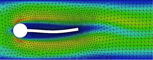
Figure 5: FSI benchmark problem

We use the data from the FSI benchmark problem in [48]. Note that this is a 2D problem. The FSI code is implemented in the framework of FEniCS[34]. The computational domain is shown in Figure 5. We have an elastic beam in a channel, where the inflow comes from the left end of the domain. We prescribe zero Dirichlet boundary conditions on the top and bottom of the channel. On the right end we use no-flux boundary condition. We use P2-P0 finite elements for the FSI system.

We use three meshes with different sizes. Numbers of degrees of freedom for these meshes are shown in Table 2.

Table 2: DoFs of the meshes

	mesh 1	mesh 2	mesh 3
DoF	11,714	45,932	181,880

The values of the parameter $r$ in M1, M2 and M3 are the same and are calculated by (18). Preconditioned GMRes is used to solve the linear systems. Although M1, M2 and M3 are originally block diagonal preconditioners, we use them in a block upper triangular fashion. Each of the diagonal blocks is solved exactly. The iteration of GMRes stops when the relative residual has magnitude less than $10^{-10}$.

In Table 3, we test the preconditioners for different meshes and time step sizes. In Table 4, we show the test results for different meshes and density ratios.

Table 3: Number of iterations for preconditioned GMRES for different time step sizes ($k=0.01,0.001,0.0001$)

	$k=0.01$				$k=0.001$				$k=0.0001$
preconditioner	M1	M2	M3	SC	M1	M2	M3	SC	M1	M2	M3	SC
mesh 1	2	20	6	16	1	19	8	10	1	26	7	9
mesh 2	2	20	6	26	1	19	8	12	1	17	8	9
mesh 3	2	24	7	54	1	23	9	21	1	27	8	11

Table 4: Number of iterations for preconditioned GMRES for varying density ratios

	$\hat{\rho}_{s}=\rho_{f}$				$\hat{\rho}_{s}=10\rho_{f}$				$\hat{\rho}_{s}=100\rho_{f}$
preconditioner	M1	M2	M3	SC	M1	M2	M3	SC	M1	M2	M3	SC
mesh 1	5	13	6	18	2	20	6	16	2	25	6	15
mesh 2	5	21	6	31	2	20	6	26	2	25	5	26
mesh 3	5	25	7	61	2	24	7	54	2	26	5	53

From the data we see that the convergence of preconditioned GMRes for M1, M2 and M3 is almost uniform and quite robust for different mesh sizes, time step sizes, and density ratios. The case with SC shows dependence on mesh sizes and the dependence becomes more significant when the time step size $k$ grows. M1 and M3 in general need significantly fewer number of iterations than M2 and are more stable than M2 for various combinations of material and discretization parameters.

Concluding remarks

In this paper, we formulate the FSI discretized system as saddle point problems. Under mild assumptions, the uniform well-posedness of the saddle point problems is shown. By adding a stabilization term or adopting a new norm for velocity, the finite element discretization of the FSI problem is also proved to be uniformly well-posed. Two optimal preconditioners are proposed based on the well-posed formulations. Our theoretical framework also provides an alternative justification for the AL-type preconditioners in the absence of the convection term. In the numerical examples, we show the robustness of these preconditioners. We use direct solves for the sub-blocks. In practice, these sub-blocks have to be inverted by iterative methods when their sizes are large. Robust preconditioners for the sub-blocks have to be considered.

References

- [1] S Badia, A Quaini, and A Quarteroni. Modular vs. non-modular preconditioners for fluid–structure systems with large added-mass effect. Computer Methods in Applied Mechanics and Engineering, 197(49-50):4216–4232, September 2008.
- [2] Santiago Badia, Annalisa Quaini, and Alfio Quarteroni. Splitting methods based on algebraic factorization for fluid-structure interaction. SIAM J. Sci. Comput., 30(4):1778–1805, 2008.
- [3] Andrew T. Barker and Xiao-Chuan Cai. Scalable parallel methods for monolithic coupling in fluid–structure interaction with application to blood flow modeling. Journal of Computational Physics, 229(3):642–659, February 2010.
- [4] Andrew T Barker and Xiao-Chuan Cai. Two-level Newton and hybrid Schwarz preconditioners for fluid-structure interaction. SIAM J. Sci. Comput., 32(4):2395–2417, 2010.
- [5] A.T. Barker and X.C. Cai. NKS for fully coupled fluid-structure interaction with application. Domain Decomposition Methods in Science and Engineering XVIII, pages 275–282, 2009.
- [6] Y. Bazilevs, M.-C. Hsu, I. Akkerman, S. Wright, K. Takizawa, B. Henicke, T. Spielman, and T. E. Tezduyar. 3D simulation of wind turbine rotors at full scale. Part I: Geometry modeling and aerodynamics. International Journal for Numerical Methods in Fluids, 65(1-3):207–235, 2011.
- [7] Y. Bazilevs, M.-C. Hsu, J. Kiendl, R. Wüchner, and K.-U. Bletzinger. 3D simulation of wind turbine rotors at full scale. Part II: Fluid–structure interaction modeling with composite blades. International Journal for Numerical Methods in Fluids, 65(1-3):236–253, 2011.
- [8] Yuri Bazilevs, Kenji Takizawa, and Tayfun E. Tezduyar. Computational Fluid-Structure Interactions: Methods and Applications. John Wiley & Sons, 2012.
- [9] Michele Benzi and Maxim A Olshanskii. An augmented Lagrangian-based approach to the Oseen problem. SIAM Journal on Scientific Computing, 28(6):2095–2113, 2006.
- [10] Michele Benzi and Maxim A Olshanskii. Field-of-values convergence analysis of augmented Lagrangian preconditioners for the linearized Navier-Stokes problem. SIAM Journal on Numerical Analysis, 49(2):770–788, 2011.
- [11] Michele Benzi, Maxim A Olshanskii, and Zhen Wang. Modified augmented Lagrangian preconditioners for the incompressible navier–stokes equations. International Journal for Numerical Methods in Fluids, 66(4):486–508, 2011.
- [12] James H Bramble, Raytcho D Lazarov, and Joseph E Pasciak. Least-squares methods for linear elasticity based on a discrete minus one inner product. Computer methods in applied mechanics and engineering, 191(8):727–744, 2001.
- [13] Franco Brezzi and Michel Fortin. Mixed and hybrid finite element methods. Springer-Verlag New York, Inc., 1991.
- [14] Xiao-Chuan Cai. Two-level Newton and hybrid Schwarz preconditioners for Fluid-Structure Interaction. SIAM J. SCI. COMPUT, 32(4):2395–2417, 2010.
- [15] P Causin, J F Gerbeau, and F Nobile. Added-mass effect in the design of partitioned algorithms for fluid-structure problems. Comput. Methods Appl. Mech. Engrg., 194(42-44):4506–4527, 2005.
- [16] Ramon Codina. Stabilized finite element approximation of transient incompressible flows using orthogonal subscales. Computer Methods in Applied Mechanics and Engineering, 191(39):4295–4321, 2002.
- [17] Paolo Crosetto. Fluid-Structure Interaction Problems in Hemodynamics: Parallel Solvers, Preconditioners, and Applications. PhD thesis, ÉCOLE POLYTECHNIQUE FÉDÉRALE DE LAUSANNE, 2011.
- [18] Paolo Crosetto, Simone Deparis, Gilles Fourestey, and Alfio Quarteroni. Parallel algorithms for fluid-structure interaction problems in haemodynamics. SIAM Journal on Scientific Computing, 33(4):1598–1622, 2011.
- [19] Paolo Crosetto, Philippe Reymond, Simone Deparis, Dimitrios Kontaxakis, Nikolaos Stergiopulos, and Alfio Quarteroni. Fluid-structure interaction simulation of aortic blood flow. Comput. & Fluids, 43:46–57, 2011.
- [20] J Donea, S Giuliani, and JP Halleux. An arbitrary Lagrangian-Eulerian finite element method for transient dynamic fluid-structure interactions. Computer Methods in Applied Mechanics and Engineering, 33(1):689–723, 1982.
- [21] J Donea, A Huerta, J.P. Ponthot, and A. Rodriguez-Ferran. Arbitrary Lagrangian–Eulerian methods. Encyclopedia of computational mechanics, pages 1–38, 2004.
- [22] Th Dunne, R Rannacher, and Th Richter. Numerical simulation of fluid-structure interaction based on monolithic variational formulations. Fundamental Trends in Fluid-Structure Interaction, 1:1–75, 2010.
- [23] M Á Fernández, J.-F. Gerbeau, and C Grandmont. A projection semi-implicit scheme for the coupling of an elastic structure with an incompressible fluid. Internat. J. Numer. Methods Engrg., 69(4):794–821, 2007.
- [24] M Á Fernández and M Moubachir. A Newton method using exact Jacobians for solving fluid–structure coupling. Computers & Structures, 83(2):127–142, 2005.
- [25] Miguel Á Fernández and Jean-Frédéric Gerbeau. Algorithms for fluid-structure interaction problems. In Cardiovascular mathematics, pages 307–346. Springer, 2009.
- [26] Luca Formaggia, Alfio Quarteroni, and Allesandro Veneziani. Cardiovascular mathematics. Number CMCS-BOOK-2009-001. Springer, 2009.
- [27] M W Gee, U Küttler, and W A Wall. Truly monolithic algebraic multigrid for fluid – structure interaction. International Journal for Numerical Methods in Engineering, 85(8):987–1016, 2011.
- [28] Vivette Girault and Pierre-Arnaud Raviart. Finite element methods for Navier-Stokes equations: theory and algorithms. NASA STI/Recon Technical Report A, 87:52227, 1986.
- [29] R Glowinski, TW Pan, TI Hesla, DD Joseph, and J Periaux. A fictitious domain approach to the direct numerical simulation of incompressible viscous flow past moving rigid bodies: application to particulate flow. Journal of Computational Physics, 169(2):363–426, 2001.
- [30] Matthias Heil. An efficient solver for the fully coupled solution of large-displacement fluid-structure interaction problems. Comput. Methods Appl. Mech. Engrg., 193(1-2):1–23, 2004.
- [31] Jaroslav Hron and Stefan Turek. A monolithic FEM/multigrid solver for an ALE formulation of fluid-structure interaction with applications in biomechanics. Springer, 2006.
- [32] Ming-Chen Hsu and Yuri Bazilevs. Fluid–structure interaction modeling of wind turbines: simulating the full machine. Computational Mechanics, 50(6):821–833, 2012.
- [33] Thomas JR Hughes, Wing Kam Liu, and Thomas K Zimmermann. Lagrangian-Eulerian finite element formulation for incompressible viscous flows. Computer methods in applied mechanics and engineering, 29(3):329–349, 1981.
- [34] Anders Logg, Kent-Andre Mardal, Garth N. Wells, et al. Automated Solution of Differential Equations by the Finite Element Method. Springer, 2012.
- [35] A Cristiano I Malossi, Pablo J Blanco, Paolo Crosetto, Simone Deparis, and Alfio Quarteroni. Implicit coupling of one-dimensional and three-dimensional blood flow models with compliant vessels. Multiscale Modeling & Simulation, 11(2):474–506, 2013.
- [36] Kent-Andre Mardal and Ragnar Winther. Preconditioning discretizations of systems of partial differential equations. Numerical Linear Algebra with Applications, 18(1):1–40, 2011.
- [37] CM Murea and S Sy. A fast method for solving fluid–structure interaction problems numerically. International journal for numerical methods in fluids, 60(10):1149–1172, 2009.
- [38] Nathan Mortimore Newmark. A method of computation for structural dynamics. In Proc. ASCE, volume 85, pages 67–94, 1959.
- [39] Maxim Olshanskii and Arnold Reusken. Grad-div stablilization for stokes equations. Mathematics of Computation, 73(248):1699–1718, 2004.
- [40] Maxim A Olshanskii and Michele Benzi. An augmented Lagrangian approach to linearized problems in hydrodynamic stability. SIAM Journal on Scientific Computing, 30(3):1459–1473, 2008.
- [41] Charles S Peskin. The immersed boundary method. Acta numerica, 11(0):479–517, 2002.
- [42] A Quaini and A Quarteroni. A semi-implicit approach for fluid-structure interaction based on an algebraic fractional step method. Math. Models Methods Appl. Sci., 17(6):957–983, 2007.
- [43] A Quarteroni. Fluid-structure interaction between blood and arterial walls. In Fundamental trends in fluid-structure interaction, volume 1 of Contemp. Chall. Math. Fluid Dyn. Appl., pages 261–289. World Sci. Publ., Hackensack, NJ, 2010.
- [44] Alfio Quarteroni, Alessandro Veneziani, and Paolo Zunino. Mathematical and numerical modeling of solute dynamics in blood flow and arterial walls. SIAM J. Numer. Anal., 39(5):1488–1511, 2001.
- [45] Tayfun E Tezduyar, Sunil Sathe, and Keith Stein. Solution techniques for the fully discretized equations in computation of fluid-structure interactions with the space-time formulations. Comput. Methods Appl. Mech. Engrg., 195(41-43):5743–5753, 2006.
- [46] T.E. Tezduyar and Sunil Sathe. Modelling of fluid–structure interactions with the space–time finite elements: solution techniques. International Journal for Numerical Methods in Fluids, 54(6-8):855–900, 2007.
- [47] S Turek and J Hron. Numerical Simulation and Benchmarking of a Monolithic Multigrid Solver for Fluid-Structure Interaction Problems with Application to Hemodynamics. Fluid Structure Interaction II:Modelling, Simulation, Optimization, 73:193, 2010.
- [48] Stefan Turek and Jaroslav Hron. Proposal for numerical benchmarking of fluid-structure interaction between an elastic object and laminar incompressible flow. Springer, 2006.
- [49] Hongwu Wang, Jack Chessa, Wing K Liu, and Ted Belytschko. The immersed/fictitious element method for fluid-structure interaction: volumetric consistency, compressibility and thin members. Internat. J. Numer. Methods Engrg., 74(1):32–55, 2008.
- [50] Xiaoping Xie, Jinchao Xu, and Guangri Xue. Uniformly-stable finite element methods for darcy-stokes-brinkman models. Journal of Computational Mathematics-International Edition, 26(3):437, 2008.
- [51] Jinchao Xu and Yunrong Zhu. Uniform convergent multigrid methods for elliptic problems with strongly discontinuous coefficients. Mathematical Models and Methods in Applied Sciences, 18(01):77–105, 2008.
- [52] Jinchao Xu and Jun Zou. Some nonoverlapping domain decomposition methods. SIAM review, 40(4):857–914, 1998.
- [53] Zhaosheng Yu. A DLM/FD method for fluid/flexible-body interactions. Journal of Computational Physics, 207(1):1–27, 2005.
- [54] Lucy Zhang, Axel Gerstenberger, Xiaodong Wang, and Wing Kam Liu. Immersed finite element method. Computer Methods in Applied Mechanics and Engineering, 193(21):2051–2067, 2004.
- [55] Walter Zulehner. Nonstandard norms and robust estimates for saddle point problems. SIAM Journal on Matrix Analysis and Applications, 32(2):536–560, 2011.