On the incidence of eclipsing Am binary systems in the SuperWASP survey

The results of a search for eclipsing Am star binaries using photometry from the SuperWASP survey are presented. The light curves of 1742 Am stars fainter than $V$ = 8.0 were analysed for the presences of eclipses. A total of 70 stars were found to exhibit eclipses, with 66 having sufficient observations to enable orbital periods to be determined and 28 of which are newly identified eclipsing systems. Also presented are spectroscopic orbits for 5 of the systems. The number of systems and the period distribution is found to be consistent with that identified in previous radial velocity surveys of ‘classical’ Am stars.

1 Introduction

Amongst the A and F stars there exists a subclass of peculiar stars called the metallic-lined (Am) stars, in which the Ca II K line is considerably weaker than would be expected from the average metallic line type (Titus & Morgan, 1940; Roman et al., 1948). These stars exhibit an apparent underabundance of calcium and scandium, overabundances of iron-group elements, and extreme enhancements of rare-earth elements (Conti, 1970). In contrast to normal A-type stars, the Am stars are slowly rotating (Wolff, 1983) with maximum $v\sin i$ values of $\sim$100 km s^-1 (Abt & Moyd, 1973). The abundance anomalies are thought to be due to radiative diffusion of elements within the stable atmospheres of these relatively slowly rotating stars (Michaud, 1970, 1980; Michaud et al., 1983).

Early spectral studies of Am stars hinted at a high fraction of spectroscopic binaries (Roman et al., 1948), while the systematic study by Abt (1961) led to the conclusion that all Am stars are members of spectroscopic binaries. Hence, it was assumed that the slow rotation of Am stars, required for radiative diffusion to occur, was the result of the reduction of rotational velocities due to tidal interaction. While there were spectroscopic orbits for many Am stars (e.g. Pourbaix et al., 2004), only a handful were known to be eclipsing (e.g. Popper, 1980; Andersen, 1991). It was this that led Jaschek & Jaschek (1990) to conclude that:

A curious fact is that among the many Am stars known (all of which are binaries) there should be many eclipsing binaries, but surprisingly very few cases are known.

Comprehensive spectroscopic radial velocity studies of carefully selected Am stars, have found a binary fraction of nearer 60–70% (Abt & Levy, 1985; Carquillat & Prieur, 2007). The period distribution shows that the majority of systems have periods $\la$ 50 days, consistent with the slow rotation being due to tidal synchronisation or pseudo-synchronization (Budaj, 1996, 1997). There are, nonetheless, systems with longer periods, suggesting that these Am stars were formed with low initial rotation velocities (North & Debernardi, 2004). The key to the Am phenomenon appears to be slow rotation and not binarity per se.

The recent Renson & Manfroid (2009) catalogue lists only 61 Am stars as eclipsing or possibly eclipsing. This represents only 1.4% of the Am stars in the catalogue. Given that a large fraction of Am stars are supposed to be in binary systems, this percentage does appear rather low. For example, in a binary with a period of $\sim$5 days (typical of many Am spectroscopic binaries), there is a $\sim$10% probability that the system should be eclipsing. Hence, there is a perhaps somewhat naïve expectation that there ought to be more eclipsing Am stars. It is this which led us to investigate the number of eclipsing systems that can be found using light curves obtained from the SuperWASP exoplanet transit survey.

2 SuperWASP observations

The WASP project is surveying the sky for transiting extrasolar planets (Pollacco et al., 2006) using two robotic telescopes, one at the Observatorio del Roque de los Muchachos on the island of La Palma in the Canary Islands, and the other at the Sutherland Station, South African Astronomical Observatory (SAAO). Both telescopes consist of an array of eight 200-mm, f/1.8 Canon telephoto lenses and Andor CCDs, giving a field of view of $7.8\degr\times 7.8\degr$ and pixel size of around 14 ″. The observing strategy is such that each field is observed with a typical cadence of the order of 10 min. WASP provides good quality photometry with a precision exceeding 1% per observation in the approximate magnitude range $9\leq V\leq 12$.

The SuperWASP data reduction pipeline is described in detail in Pollacco et al. (2006). The aperture-extracted photometry from each camera on each night are corrected for primary and secondary atmospheric extinction, instrumental colour response and system zero-point using a network of stars with colours defined in the Tycho-2 catalogue. Even though the WASP bandpass extends further into the red, the resultant pseudo-$V$ magnitudes are comparable to Tycho $V$ magnitudes. Additional systematic errors affecting all the stars are identified and removed using the SysRem algorithm of Tamuz et al. (2005).

We have selected Am stars from the Renson & Manfroid (2009) catalogue for which we have data in the WASP archive and when individual light curves have at least 1000 data points (i.e. for a single camera and during a single season). In addition, we rejected any stars with magnitudes brighter than $V=8.0$, in order to avoid the most significant effects of saturation in the WASP images. A total of 1742 stars were selected for light curve analysis, which is 55% of the Am stars of $V=8.0$ or fainter in Renson & Manfroid (2009) and 40% of all the Am stars in the catalogue.

3 Light curve analysis

The light curves of the target stars were analysed using the WASP Project’s hunter program (Collier Cameron et al., 2006), which is an adaptation of the Box Least Squares algorithm of Kovács et al. (2002). The algorithm computes $\chi^{2}$ values of transit model light curves using a box-shaped model that is slid over the observed light curve. The period-searching range was from 1 to 50 days. Each individual light curve was then folded on the periods of the 5 most significant $\chi^{2}$ values and visually inspected for the presence of eclipses.

From the survey of 1742 Am stars, fainter than $V$ = 8.0, 70 eclipsing systems were found, of which 28 are previously unreported detections (Table 1) and 4 are suspected eclipsing systems (Table 2), but with too few eclipses to confirm their eclipsing status or to determine an orbital period. This brings the total number of known eclipsing Am stars to around 100. Around 4% of the Am stars in our sample have been found to exhibit eclipses.

Table 1: Eclipsing Am binaries. Columns 5 and 6 give the depths, in mmag., of primary (Min i) and secondary (Min ii) minima. Column 7 gives the phase of secondary minimum ($\phi_{\mbox{{ii}}}$) if different from 0.50. Column 8 gives the binary classification. A dagger (†) indicates that there is a possible $P\times 2$ uncertainty from the WASP light curve. For previously known systems Column 10 gives the GCVS designation where available, otherwise either an ASAS designation (Pojmanski, 2002) or a literature reference.

Renson	Name	Spec. Type	$P_{\rm orb}$ (d)	Min I	Min II	$\phi_{\mbox{{ii}}}$	Class	Dilution	Known System
3330	HD 12950	A4mA8	2.39831	0.029	0.018	…	Ell	0.55
3590	HD 14111	A0mF2	1.63078	0.042	0.009	…	EA	0
3750	HD 15082	A5m	1.21988	0.017	…	…	Det †	0.08	Collier Cameron et al. (2010)
4290	HD 16903	A3mF2	1.51947	0.050	0.014	…	EA	0
4660	HD 18597	A1mF0	2.78071	0.681	0.522	…	Det	0	XY Cet
5685	HD 275604	A4mF0?	7.16050	0.555	0.149	0.51	EA	0	AB Per
5982	TYC 3725-496-1	A2m?	2.41394	0.055	0.027	0.52	Ell	0.05
6720	HD 26481	A2mF2	2.38318	0.243	0.209	…	Det	0	AE Hor
7310	HD 28451	B9m	6.66372	0.328	0.154	…	Det	0	ASAS 042815-2306.1
7730	HD 30050	A5m?	39.28272	0.817	0.073	0.65	Det	0	RZ Eri
8215	HD 32239	A5mF?	8.79590	0.234	0.099	…	Det	0
8973	HD 243104	A5m	1.88678	0.317	0.040	…	EA	0.09	V606 Aur
9237	HD 243875	A2m?	2.85625	0.111	0.052	…	Det	0.35
9318	TYC 1848-800-1	A5m?	11.11333	0.206	0.127	…	Det	0.01
9410	HD 36412	A7mF4	16.78729	0.552	0.124	0.49	Det	0	EY Ori
9458	HD 244709	A3m?	2.25868	0.059	0.017	…	EA/EB	0.14
10016	HD 245819	A3m	5.43090	0.476	0.447	0.56	Det	0.04	V1260 Tau
10310	HD 38303	A2mA9	1.21672	0.295	0.050	…	EA	0.01	WZ Pic
10326	HD 38390	A3mF4	3.72095	0.170	0.012	…	EA	0	ASAS 054507-0856.8
10336	HD 38453	A1mF0	2.52600	0.203	0.025	…	EA	0	ASAS 054602+0212.1
10387	HD 247657	A7m	3.16130	0.483	0.317	0.52	W UMa	0.04	NSVS 6994211
10689	HD 249628	A2m	1.08374	0.140	0.097	0.59	W UMa?	0.09	NSVS 7022747
10892	HD 250443	A3m	2.17543	0.031	0.016	0.53	Ell/Graz	0.01
11100	HD 41491	A1mA5?	4.03751	0.151	0.056	…	Det	0
11387	HD 253252	A4mF1	0.81098	0.285	0.148	…	W UMa?	0.02	V2787 Ori
11470	HD 42968	A0mF1	2.87213	0.473	0.138	…	EA?/Det?	0	IO CMa
14040	HD 50992	A2mA7	1.56695	0.105	0.045	…	EA/Ell	0.24
14850	HD 54011A	A1mF0?	3.97948	0.084	0.008	…	Det †	0.02
15034	HD 55228	F2m Sr	7.53921	0.172	0.095	…	Det?	0	V422 Gem
15190	HD 55822A	A3mF5	5.12290	0.062	…	…	Det †	0
15445	HD 56587	A3mF2	5.76059	0.520	0.462	…	Det	0	V339 Gem
18505	HD 67093	A3mF0	4.33586	0.340	0.319	…	Det	0	V871 Mon
21400	HD 76320	A2m	7.77292	0.193	0.009	…	Det †	0
22860	HD 80343	A3mA9	7.90058	0.076	0.066	0.66	Det	0
25020	HD 87374	A0m?	6.62845	0.009	…	…	Det †	0.05
25070	HD 87450	A1mF2	6.71489	0.228	0.214	0.58	Det	0	ASAS 100421-3319.0
25880	HD 90029	A5m $\delta$ Del	9.86030	0.074	0.052	…	Det	0	BY Ant
28850	HD 100376	F0m? $\delta$ Del?	1.64361	0.046	0.046	…	Ell/Cont/grazing	0	ASAS 113257-2737.4
29290	HD 101681	A3m?	3.29220	0.188	0.179	…	Det †	0.05	ASAS 114149-4229.5
30090	HD 104120	A3mF2	4.34862	0.155	0.155	…	Det †EA?	0.01
30110	HD 104186	A5m?	4.31449	0.029	…	…	Det	0
30457	HD 105376	A2mA8	11.94200	0.069	…	…	Det †	0
30650	HD 106046	A2mF0	18.12101	0.168	…	…	Det †	0
30820	HD 106546	A0m	2.87025	0.025	0.006	…	EA	0
34770	HD 120777	A2mF0	2.54163	0.020	0.005	0.57	EA	0.03
35000	HD 121788	A2 Sr Cr or Am?	10.28606	0.146	…	…	Det †	0	ASAS 135817-3004.5
36660	HD 128806	A1mF2	16.36534	0.559	0.257	0.44	Det	0.02	ASAS 143944-2837.2
37220	HD 130922	F5m?	5.79311	0.120	0.117	…	Det †	0.34
37610	HD 132515A	F8 Sr or $\delta$ Del	3.23869	0.236	0.314	…	Det	0.18	IU Lup
38180	HD 134477	A1mA6	6.14445	0.075	0.035	…	EA	0	OY Lup
38500	HD 135492	A2mA9	3.99382	0.090	0.020	…	Det	0.04
40350	HD 142232	A3mF2	7.06875	0.103	…	…	Det †	0
40780	HD 143926	A5mF0	6.93480	0.175	0.170	…	Det	0
40910	HD 144396	A1mF0	11.11629	0.353	0.349	0.47	Det	0.11	V1046 Sco
42906	HD 151604	A0m	19.69874	0.285	…	…	Det †	0.04	V916 Her
44140	HD 156965	A5mA9	2.05984	0.630	0.403	…	Det	0	TX Her
49380	HD 177022	F4m?	5.02043	0.096	0.049	0.56	Det	0.27
51506	HD 186753	A2mF0?	1.91955	0.018	0.004	0.44	Det	0	Bentley et al. (2009)
56310	HD 201964	A2m	2.69592	0.413	0.354	…	Det	0.03	DG Mic
56830	HD 204038	A3mF0	0.78582	0.321	0.286	…	Ell/Cont/grazing	0.03	V1073 Cyg
57845	HD 208090	A2m $\delta$ Del?	2.44660	0.176	0.048	…	EA?	0	Wraight et al. (2011)
58170	HD 209147	A2mA4	1.60471	0.947	0.338	…	Det	0	CM Lac
58256	HD 209385	A3mF3	2.96733	0.140	0.062	…	Det	0.05
59780	HD 216429	A1mA8?	7.35140	0.592	0.498	0.51	Det	0.04	V364 Lac
60640	HD 221184	A5m?	5.46091	1.299	0.081	…	EA	0	AN Tuc
61280	TYC 6408-989-1	A4m or A5 Sr?	0.47080	0.373	0.178	…	Ell/Cont/grazing	0	ASAS J235103-1904.5

Table 2: Suspected eclipsing Am binaries.

Renson	Name	Sp. Type	Notes
7360	HD 28617	A0mA5 ?	Eclipse, JD 4396.64, depth 0.17 mag.
9701	HD 245224	A2m	Egress, JD 4083.50, depth 0.1 mag.
36950	HD 129575	F0m $\delta$ Del	Possible egress, JD 3891.20, depth 0.2 mag.
61470	HD 224401	A4mF2	Egress, JD 5399.40, depth 0.1 mag.

3.1 Cross-checking with AAVSO

In order to check whether any known eclipsing systems had been missed, a cross-check with AAVSO (Watson, 2006) was performed. All but two of the known systems were recovered in the WASP data. The first system, Renson 5740 (BD+44 765) is listed as an XO false positive (Poleski et al., 2010) with an eclipse depth of 0.018 mag. and duration of 3.37 hours. There is only a single, rather noisy, WASP light curve and folding on their ephemeris, shows no sign of any transits. Furthermore, only two transits would have occurred within the WASP light curve, which is less than the minimum 3 required for detection of a period. Thus, even if the eclipses had been found, the period would have been unknown. The other system, Renson 34764 (HD 120727) is a suspected eclipsing system (Hooten & Hall, 1990). However, the 3 good quality WASP light curves do not show any evidence of eclipses. Hence, we conclude that this is not an eclipsing system.

3.2 Systems also showing pulsations

In Smalley et al. (2011) we found that approximately 14% of Am stars pulsate with amplitudes $\ga 1$ mmag.. Hence, we might expect some of the binary systems to show evidence of pulsations. A search for pulsations was undertaken using the residuals to the fitted light curves.

Two of the binary systems already have known pulsations. Renson 3750 (HD 15082) was found to exhibit $\delta$ Scuti pulsations at the milli-magnitude level (Herrero et al., 2011), but these are not detectable in the WASP data. Renson 5685 (HD 275604; AB Per) was reported to have 10 mmag. pulsations in the $B$ band with a frequency of 5.106 d^-1 (Kim et al., 2003). There is a $\sim$6 mmag. peak in the periodogram of the residuals for the multi-season combined light curve with a frequency of around 5.116 d^-1, which confirms the previous detection.

Of the remaining systems, Renson 8973 (HD 243104; V606 Aur) was found to clearly exhibit pulsations. This system has 11.9 mmag. $\delta$ Scuti-type pulsations with a frequency of 23.572 d^-1. Another system, Renson 10310 (HD  38303; WZ Pic) shows 1.5 mmag. pulsations with a frequency of 22.783 d^-1, but individual seasons show this period at $\pm$1 d^-1 aliases. Another system, Renson 30110 (HD 104186) shows some evidence for excess power in the individual light curves at the 1$\sim$2 mmag. level around 10 d^-1. However, none of them yield consistent frequencies. Thus we conclude that the hints of pulsations in Renson 30110 are probably spurious.

4 Spectroscopic observations

Spectroscopic observations of five of the Am binary systems were obtained at the 2.15m telescope at the Complejo Astronómico el Leoncito (CASLEO) on the nights between the 2009 June 12 and the 2009 June 18. A Tektronik 1024$\times$1024 CCD and the REOSC echelle spectrograph with the either the grating 580 (400 l mm^-1) or grating 260 (600 l mm^-1) as detailed in Table 3. The spectral resolution was 25600 and the integration times were 1800s.

Table 3: Spectrograph setting for each night

Day	Grating	Angle	Wavelength Range
12	260	8°25′	3663–5264
13	260	9°50′	4396–5968
14	260	9°10′	4053–4943
15	580	7°00′	3940–6305
16	580	7°00′	3940–6305
17	260	10°30′	4888–6485
18	260	9°10′	4053–4943

Data reduction was performed using iraf (Tody, 1986, 1993). Master bias and flat field frames were obtained by combining sets of 50 individual images. The stellar spectra were bias subtracted and divided by the normalized master flat field. They were then cleaned for cosmic rays and scattered light corrected. The echelle orders were extracted to produce spectra for each individual order and wavelength calibrated using ThAr lamp spectra.

Radial velocities were obtained by cross-correlation with synthetic spectra generated using uclsyn (Smith & Dworetsky, 1988). The heliocentric values are given in Table 4.

Table 4: Heliocentric radial velocity measurements for five Am binary systems. The uncertainty in RV is 5 km s^-1.

HJD-2450000	RV1	RV2	RV3
Renson 25070 (HD 87450)
4995.482959	+4	…
4996.475654	+88	$-$80
4998.480418	+6	…
4999.490138	$-$60	+64
5000.501385	$-$68	+75
5001.493102	$-$36	+44
Renson 34770 (HD 120777)
4995.549946	$-$37
4996.565241	$-$15
4998.534940	$-$18
5000.559216	$-$30
5001.576971	$-$12
Renson 36660 (HD 128806)
4995.605844	$-$57	+20
4996.619294	$-$36	$-$1
4997.589355	$-$19	…
4998.650717	$-$21	…
4999.570940	$-$16	…
5001.673912	$-$1	$-$51
Renson 49380 (HD 177022)
4995.7364532	+138	$-$198	$-$45
4996.7481885	+35	$-$142	$-$44
4998.7799882	$-$95	+22	$-$48
4999.7443681	$-$103	+24	$-$46
5001.7471764	+35	$-$135	$-$41
Renson 51506 (HD 186753)
4995.810117	$-$2
4997.798468	$-$7
4998.851621	$-$51
4999.819895	$-$17
5001.855602	$-$16

5 Spectroscopic orbits

The light curves of many of the systems are extensively covered by SuperWASP observations, making a preliminary analysis of individual objects worthwhile. We also possess radial velocity (RV) measurements for 5 systems, opening the possibility of obtaining a full set of physical properties.

For the light curve analysis we chose to use the jktebop code (Southworth et al., 2004; Southworth, 2008), which is suitable for detached eclipsing binaries (dEBs) with only moderately distorted stars. jktebop has recently been extended to include the simultaneous fitting of one light curve and RVs for both components (Southworth, 2013). The sizes of the primary and secondary star are parametrised using the fractional radii, $r_{\rm A}=\frac{R_{\rm A}}{a}$ and $r_{\rm B}=\frac{R_{\rm B}}{a}$, where $a$ is the orbital semi-major axis and $R_{\rm A}$ and $R_{\rm B}$ are the true radii of the stars. The main parameters of the fit are the sum and ratio of the fractional radii, $r_{\rm A}+r_{\rm B}$ and $k=\frac{r_{\rm B}}{r_{\rm A}}=\frac{R_{\rm B}}{R_{\rm A}}$, the orbital inclination $i$, the central surface brightness ratio of the two stars $J$, the orbital period $P_{\rm orb}$ and the time of primary mid-eclipse $T_{0}$.

In the cases of eccentric orbits the orbital eccentricity, $e$, and longitude of periastron, $\omega$, were included using the combination terms $e\cos\omega$ and $e\sin\omega$. The value of $e\cos\omega$ is closely related to the orbital phase at which the secondary eclipse occurs, so is usually measured precisely. On the other hand, $e\sin\omega$ is less well tied down as it primarily determines the ratio of the durations of the eclipses. The precision of the measurements of $e\cos\omega$ and $e\sin\omega$ are significantly improved when RVs can be included as well as light curves in a solution. When RVs were available we also fitted for one or both of the velocity amplitudes, $K_{\rm A}$ and $K_{\rm B}$, as well as the systemic velocities of the star.

We checked for contaminating ‘third light’, $L_{3}$, from additional stars in the same point spread function as our target stars. The value of $L_{3}$ was set to zero unless there was clear evidence of its existence. We also fitted for the out-of-transit magnitudes of the stars and in some cases the size of the reflection effect. Limb darkening was implemented using the linear law with appropriate coefficients, and reasonable choices of the coefficients have a negligible effect on our results.

As a first step for each object, we determined an initial orbital ephemeris manually and then ran preliminary fits to its light curve alone. An iterative 3$\sigma$ clip was used to remove discrepant data points affected by weather or instrumental problems. We then assigned the same measurement error to every data point of such a size as to yield a reduced $\chi^{2}$ value of unity for the best fit. The radial velocities were then added into the solution and their error bars were adjusted to yield reduced $\chi^{2}$ values near unity for individual data sets.

Uncertainties in the deduced parameters were assessed using Monte Carlo and residual-permutation simulations (Southworth et al., 2004; Southworth, 2008). 1$\sigma$ error bars were estimated by marginalising over the parameter distributions for these simulations. In line with previous experience with SuperWASP data we find that the residual-permutation uncertainties are typically twice as large as the Monte Carlo uncertainties, and we quote the larger of the two alternatives for each measured parameter.

Table 5: Measured properties of the systems with RV measurements.

Parameter	Renson 25070	Renson 34770	Renson 36660	Renson 49380	Renson 51506
$P_{\rm orb}$ (d)	6.714890 $\pm$ 0.000011	2.541648 $\pm$ 0.000016	16.36534 $\pm$ 0.00011	5.02068 $\pm$ 0.00003	1.919549 $\pm$ 0.000019
$T_{0}$ (HJD-2450000)	4145.5389 $\pm$ 0.0007	4546.9679 $\pm$ 0.0021	4614.3659 $\pm$ 0.0015	3903.5220 $\pm$ 0.0015	4272.4863 $\pm$ 0.0034
$r_{\rm A}+r_{\rm B}$	0.2006 $\pm$ 0.0005	0.255 $\pm$ 0.005	0.0986 $\pm$ 0.0016	0.174 $\pm$ 0.014	0.390 $\pm$ 0.038
$k$	1.0 fixed	0.0987 $\pm$ 0.0022	1.038 $\pm$ 0.05	0.9 fixed	0.11157 $\pm$ 0.0084
$i$	83.90 $\pm$ 0.03	90.0 $\pm$ 1.5	88.13 $\pm$ 0.07	84.7 $\pm$ 1.6	75.0 $\pm$ 3.8
$J$	1.05 $\pm$ 0.02	0.070 $\pm$ 0.022	0.90 $\pm$ 0.07	0.78 $\pm$ 0.32	0.187 $\pm$ 0.004
$e\cos\omega$	0.131 $\pm$ 0.001	0.106 $\pm$ 0.003	$-$0.082 $\pm$ 0.001	0.085 $\pm$ 0.001	$-$0.092 $\pm$ 0.024
$e\sin\omega$	0.036 $\pm$ 0.006	0.224 fixed	0.420 $\pm$ 0.014	0.117 $\pm$ 0.032	$-$0.110 $\pm$ 0.130
$K_{\rm A}$ (km s-1)	87 $\pm$ 4	15 $\pm$ 2	49 $\pm$ 9	76.5 $\pm$ 2.2	23.2 $\pm$ 2.5
$K_{\rm B}$ (km s-1)	86 $\pm$ 5		65 $\pm$ 7	92.2 $\pm$ 2.5
Light ratio	1.05 $\pm$ 0.02	0.00068 $\pm$ 0.00003	0.97 $\pm$ 0.10	0.63 $\pm$ 0.26	0.0055 $\pm$ 0.0034
$e$	0.1358 $\pm$ 0.0016	0.2476 $\pm$ 0.0013	0.428 $\pm$ 0.013	0.145 $\pm$ 0.026	0.15 $\pm$ 0.10
$\omega$ (degrees)	16 $\pm$ 3	65 $\pm$ 2	101.1 $\pm$ 0.4	54 $\pm$ 8	129 $\pm$ 27
$a$ ($R_{\sun}$)	23.0 $\pm$ 1.1		331 $\pm$ 5	16.6 $\pm$ 0.5
$M_{\rm A}$ ($M_{\sun}$)	1.8 $\pm$ 0.3		1.01 $\pm$ 0.4	1.34 $\pm$ 0.11	1.83
$M_{\rm B}$ ($M_{\sun}$)	1.8 $\pm$ 0.2		0.81 $\pm$ 0.4	1.11 $\pm$ 0.09	0.223
$R_{\rm A}$ ($R_{\sun}$)	2.31 $\pm$ 0.10		1.611 $\pm$ 0.23	1.52 $\pm$ 0.13	2.93
$R_{\rm B}$ ($R_{\sun}$)	2.31 $\pm$ 0.10		1.671 $\pm$ 0.22	1.37 $\pm$ 0.12	0.333
$\log g_{\rm A}$ (cgs)	3.97 $\pm$ 0.02		4.052 $\pm$ 0.05	4.20 $\pm$ 0.06
$\log g_{\rm B}$ (cgs)	3.97 $\pm$ 0.02		3.902 $\pm$ 0.08	4.21 $\pm$ 0.06

5.1 Renson 25070 (HD 87450)

Figure 1: Observed light and RV curves of Renson 25070 (points) compared to the best fit found using jktebop (lines). For presentation purposes only, the WASP light curve has been binned into 400 phase bins.

This object shows eclipses 0.25 mag deep on an orbital period of 6.7 d. The secondary eclipse is almost as deep as the primary, showing that the two stars have almost the same surface brightness and are probably very similar stars. The stars are well-detached and in a mildly eccentric orbit: secondary eclipse occurs at phase 0.583. We obtained six spectra of Renson 25070 on almost-successive nights. Two were taken when the velocities of the stars were similar and their spectral lines were not resolved, but the remaining four were taken when the lines were nicely separated. All six RVs were used for each star, with the ones near conjunction down-weighted by a factor of ten. A total of 18 137 data points are included in the light curve.

The partial eclipses combined with two similar stars led to a solution which was poorly defined, so we fixed the ratio of the radii to be $k=1$ for our final solution. The measured mass ratio is consistent with unity, which supports this decision. Both stars have a mass of 1.8 $M_{\sun}$ and a radius of 2.3 $R_{\sun}$, so are slightly evolved. The fits to the light and RV curves are shown in Fig. 1 and the fitted parameters are given in Table 5. The masses, radii and surface gravities have the symbols $M_{\rm A}$ and $M_{\rm B}$, $R_{\rm A}$ and $R_{\rm B}$, and $\log g_{\rm A}$ and $\log g_{\rm B}$, respectively. Note that the uncertainties are underestimated because we have imposed the constraint $k=1$ on the solution.

5.2 Renson 34770 (HD 120777)

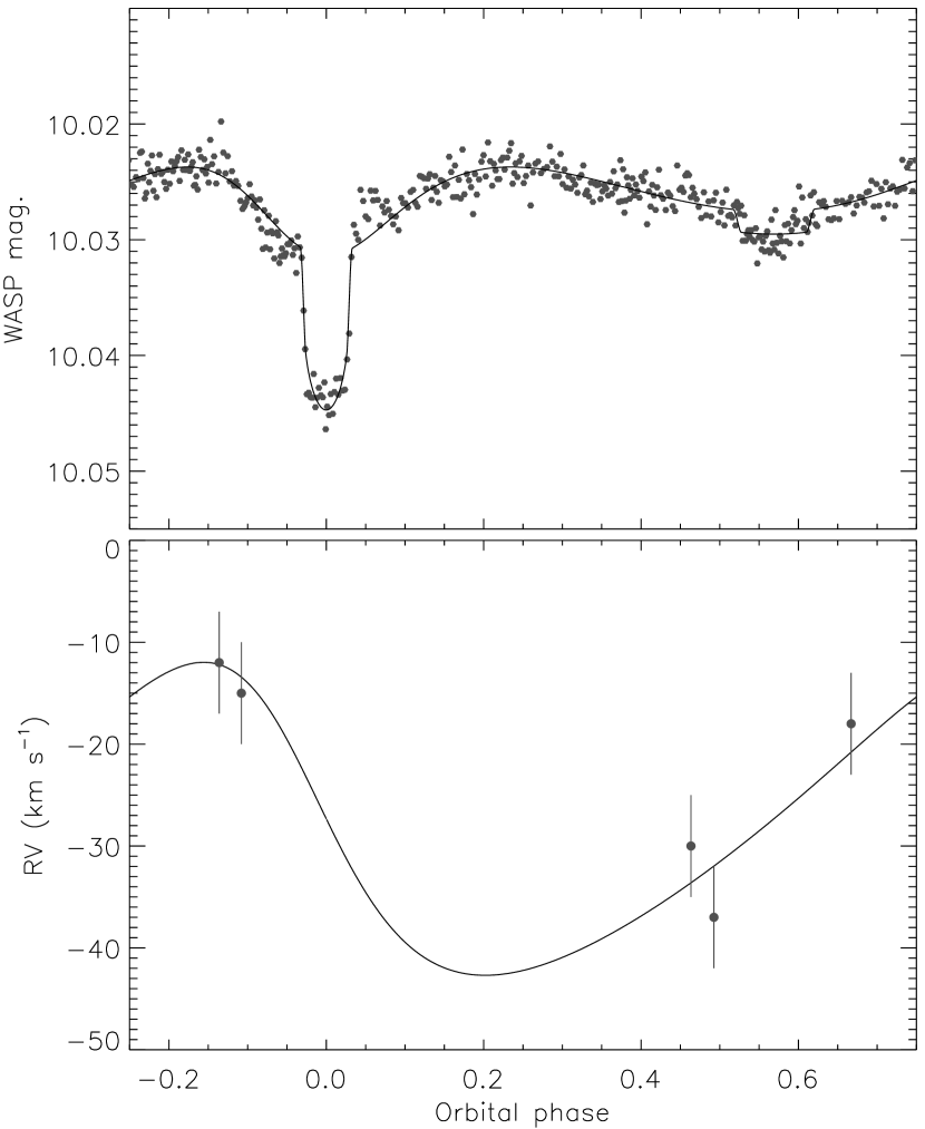
Figure 2: Observed light and RV curves of Renson 34770 (points) compared to the best fit found using jktebop (lines). For presentation purposes only, the WASP light curve has been binned into 400 phase bins.

Renson 34770 shows shallow eclipses on a period of 2.5 d. The primary eclipse is securely detected with a depth of 0.014 mag., but the secondary eclipse is only speculatively detected with a depth of 0.002 mag.. The orbit is moderately eccentric and secondary eclipse occurs at phase 0.569. The secondary star is a low-mass object with a radius ten times smaller than that of the primary. Five RVs were measured for the primary star, but the secondary could not be detected in the spectrum. A joint fit to the light curve and RVs of the primary star was poorly determined, so we fixed $e\cos\omega=0.224$ to obtain a reasonable solution indicative of the properties of the system. This solution is shown in Fig. 2 and the fitted parameters are in Table 5.

A definitive analysis will require high-quality photometry to measure the depth and shape of the primary and specifically the secondary eclipse. Whilst the SuperWASP light curve contains 13 144 data points, they have an rms of 7 mmag versus the fitted model. The secondary component is not of planetary mass – it is massive enough to induce tidal deformation of the primary star which manifests as ellipsoidal variations easily detectable in the SuperWASP light curve.

5.3 Renson 36660 (HD 128806)

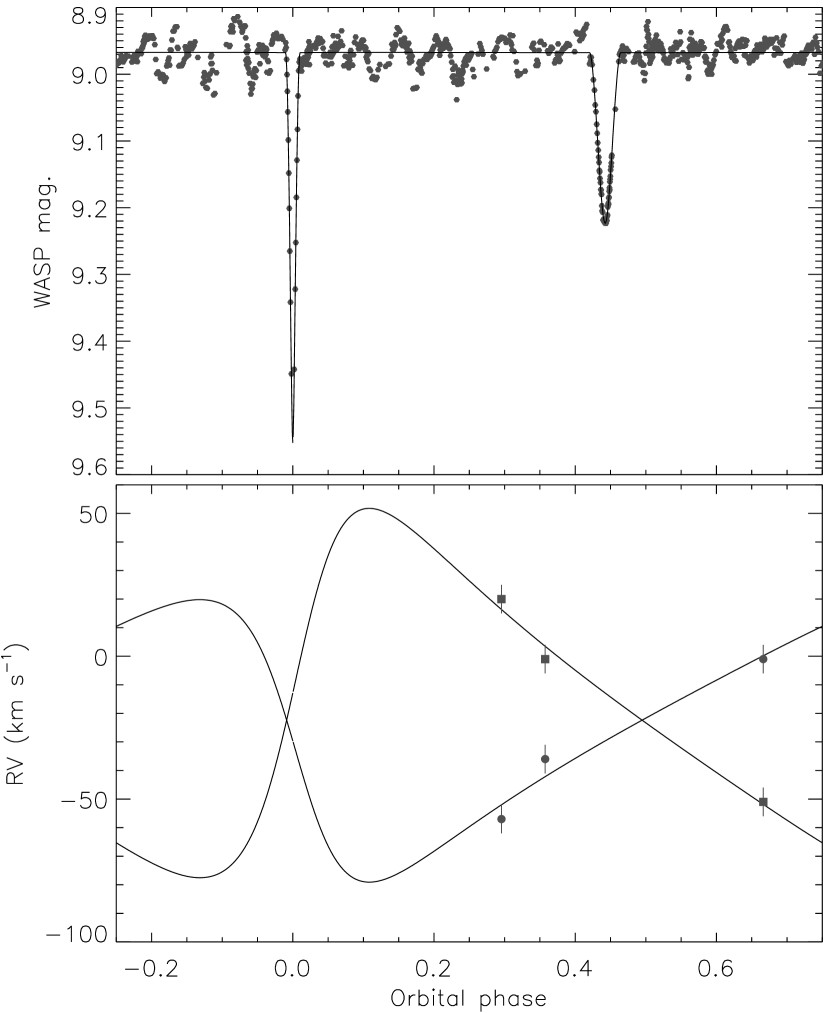
Figure 3: Observed light and RV curves of Renson 36660 (points) compared to the best fit found using jktebop (lines). For presentation purposes only, the WASP light curve has been binned into 1000 phase bins.

The SuperWASP light curve of Renson 36660 has 9089 data points and shows significant systematic trends due to the brightness of the system putting it near the saturation limit. Its orbit is eccentric – the secondary eclipse is much longer than the primary and occurs at phase 0.442 – with a period of 16.4 d. The eclipses are partial and are deep at 0.6 mag and 0.3 mag, respectively. We obtained six spectra and were able to measure RVs from three of them. These RVs were included in the fit (Fig. 3), yielding the full physical properties of the system (Table 5).

The masses we find (1.0 and 0.8 $M_{\sun}$) are significantly too low for the spectral type of the system (A1m), an effect which is likely due to spectral line blending (e.g. Andersen, 1975). Three of our spectra show fully blended lines and were not measured for RV. Two more of the spectra suffer from significant line blending, and only one spectrum (that at phase 0.3) has cross-correlation function peaks from the two stars which are clearly separated. An investigation and mitigation of this problem could be achieved by a technique such as spectral disentangling (Simon & Sturm, 1994), but this requires significantly more spectra than currently available so is beyond the scope of the present work.

We crudely simulated the effects of line blending by moving each of the four RVs from the blended spectra by 5 km s^-1 away from the systemic velocity. The resulting solution gave lower RV residuals and masses of 1.5 and 1.2 $M_{\sun}$, showing that a modest amount of blending can easily move the measured masses to more reasonable values. For the current work we present our solution with the measured RVs rather than those with an arbitrary correction for blending, and caution that much more extensive observational material is required to obtain the properties of the system reliably.

The physical properties of the stars in our preliminary solution were very uncertain, in particular the light ratio between the two objects. The main problem was the well-known degeneracy between $k$ and $J$ measured from the deep but partial eclipses, exacerbated by correlations with $e\sin\omega$ for this eccentric system (e.g. Popper & Etzel, 1981). We therefore measured a spectroscopic light ratio of $0.8\pm 0.2$ from the line strengths in the spectrum which shows well-separated lines, and applied it to the jktebop solution using the method of Southworth et al. (2007). This makes the radii of the two stars much more precise, but they will still be too small because the line blending causes an underestimation of the orbital semimajor axis as well as the stellar masses. The correlated noise in the SuperWASP light curve results in large uncertainties in the measured photometric parameters.

5.4 Renson 49380 (HD 177022)

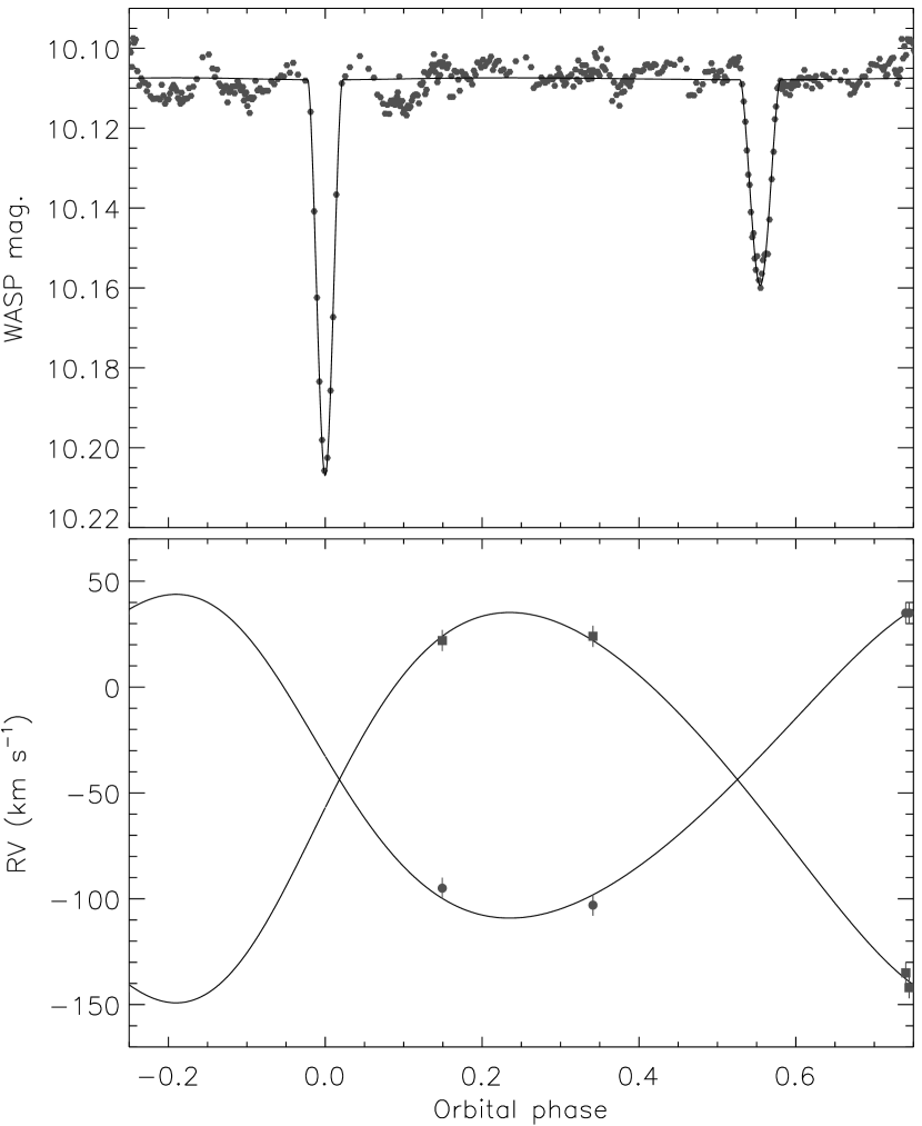
Figure 4: Observed light and RV curves of Renson 49380 (points) compared to the best fit found using jktebop (lines). For presentation purposes only, the WASP light curve has been binned into 400 phase bins.

The SuperWASP light curve of this object (8029 data points) shows shallow eclipses of depth 0.10 and 0.05 mag., respectively. The 5.0 d orbit is eccentric, and secondary minimum occurs at phase 0.555. It is in a crowded field and many fainter stars are positioned inside the photometric aperture. We therefore allowed for third light when fitting the light curve, finding a value of $L_{3}=0.64\pm 0.06$.

We obtained four spectra of Renson 49380, all taken when the velocity separation of the two stars was at least 100 km s^-1. The best solution to all data has an rms residual of 8 mmag. for the photometry and 3 km s^-1 for the RVs. This is plotted in Fig. 4 and the parameters are given in Table 5. The parameters of a free fit are poorly defined because $L_{3}$ is strongly correlated with $k$, so we set $k$ to a reasonable value of 0.9 to obtain a nominal solution.

The stars have masses of 1.3 and 1.1 $M_{\sun}$ and radii of 1.5 and 1.4 $R_{\sun}$. These numbers are rather modest, but agree with the $T_{\mathrm{eff}}$ = 6000 K suggested by colour indices of the system. The stars are slightly too late-type to be Am stars, so this could be a case of misclassification of a composite spectrum as a metal-rich spectrum.

5.5 Renson 51506 (HD 186753)

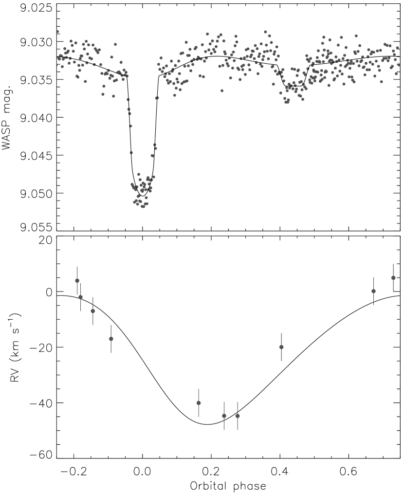
Figure 5: Observed light and RV curves of Renson 51506 (points) compared to the best fit found using jktebop (lines). For presentation purposes only, the WASP light curve has been binned into 400 phase bins.

This star was identified as a dEB consisting of an A star and an M star by Bentley et al. (2009), who presented eight RV measurements of the A star and combined these with the SuperWASP light curve to obtain the physical properties of the system. We have revisited this system because further SuperWASP data (now totalling 9896 points) and five more spectra are available. The light curve shows a clear detection of the secondary minimum (Fig. 5), with a significance of 3.4$\sigma$, at orbital phase 0.441.

The RVs of Renson 51506 are relatively poorly defined, due to the high rotational velocity of the primary star ($v\sin i$ = 65 $\pm$ 5 km s^-1; Bentley et al. 2009). We rejected the single HARPS measurement from Bentley et al. (2009), and also two of our own measurements which were discrepant with both the best fit and a CORALIE RV obtained at the same orbital phase. This allowed us to obtain a determinate solution of the light and RV curves (Fig. 5 and Table 5). Those parameters also measured by Bentley et al. (2009) are all within 1$\sigma$ of the values we find.

Whilst we lack RVs of the secondary star, we were able to estimate the full physical properties of the system by finding the $K_{\rm B}$ which reproduces the primary star mass of $M_{\rm A}=1.794$ $M_{\sun}$ obtained by Bentley et al. (2009) from interpolation in theoretical models. Adopting $K_{\rm B}=187.9$ km s^-1 gives masses of 1.8 and 0.22 $M_{\sun}$ and radii of 2.9 and 0.33 $R_{\sun}$ for the two stars. This is unsurprisingly in good agreement with the values found by Bentley et al. (2009). The secondary star is of very low mass and has a radius too large for theoretical predictions; such discrepancies have been recorded many times in the past (e.g. Hoxie, 1973; Ribas, 2006; López-Morales, 2007). Near-infrared spectroscopy of the Renson 51506 system could allow measurement of the orbital motion of the secondary star, which together with the existing light curve would yield the full physical properties of the system without reliance on theoretical models. The secondary star could then be used as a probe of the radius discrepancy in the crucial 0.2 $M_{\sun}$ mass regime.

5.6 Other objects

RVs are not available for the other Am-type EBs studied in this work. We modelled the light curves of these objects with the primary aim of determining reliable orbital periods to facilitate population studies and follow-up observations. After obtaining preliminary solutions we performed iterative 3$\sigma$ rejection of discrepant points to arrive at a light curve fit for more detailed analysis.

A small fraction of the systems show strong tidal interactions which deform the stars beyond the limits of applicability of the jktebop code. Reliable solutions could be obtained by the use of a more sophisticated model, such as implemented in the Wilson-Devinney code (Wilson & Devinney, 1971), at the expense of much greater effort and calculation time. This work is beyond the scope of the paper; in these cases jktebop is still capable of returning the reliable orbital ephemerides which are our primary goal when modelling the light curves.

6 Detection probability

In order to assess whether the observed fraction of eclipsing Am stars is consistent with the expected fraction of Am binaries, we need to determine the detection probability. Of the 1742 stars in our sample, 282 have $uvby\beta$ photometry which gives an average $T_{\mathrm{eff}}$ = 7520$\pm$580 K using the calibration of Moon & Dworetsky (1985). Hence, in the following, we assume that a typical Am star is around $T_{\mathrm{eff}}$ = 7500 K, with $R=1.7\,R_{\sun}$, $M=1.7\,M_{\sun}$ and $L=7\,L_{\sun}$. We will consider two scenarios; two identical $1.7\,R_{\sun}$ stars and the case of a dark companion with radius $\sim$0.2 $R_{\sun}$. In both cases, we assume that the orbits are circular.

6.1 Eclipsing probability

The probability of an eclipse being seen from the Earth is given by

$$p_{\rm eclipse}=\frac{R_{1}+R_{2}}{a},$$

where $R_{1}$ and $R_{2}$ are the stellar radii of the two stars and $a$ is orbital separation in same units. The above criterion is purely geometric and does not take into account the effects of limb-darkening or noise on the detection of shallow eclipses. Hence, the maximum sky-projected separation of the centres of the two stars which will lead to a detectable eclipse will be less than $R_{1}+R_{2}$ by an amount $\delta R$. The probability of detectable eclipse is therefore,

$$p_{\rm eclipse}=\frac{R_{1}+R_{2}-\delta R}{a}.$$

Assuming a linear limb-darkening law with $\epsilon=0.6$ and a minimum detectable eclipse depth of 0.01 mag., we get $\delta R$=0.28 $R_{1}$ and $\delta R$=0.15 $R_{1}$, for a 0.1 $R_{1}$ dark companion and two identical stars, respectively. Using Kepler’s 3rd Law, we get

$$p_{\rm eclipse}=0.23756\frac{(R_{1}+R_{2}-\delta R)}{\sqrt[3]{P_{\rm orb}^{2}(M_{1}+M_{2})}},$$

where $R_{1}$, $R_{2}$ and $\delta R$ are in $R_{\sun}$, $M_{1}$ and $M_{2}$ are in $M_{\sun}$ and $P_{\rm orb}$ in days. An uncertainty of $\pm$0.3$R_{\sun}$ and $\pm$0.3$M_{\sun}$ in stellar radii and masses, yields an uncertainty in $p_{\rm eclipse}$ of approximately 10%, with the uncertainty being dominated by that on the stellar radius.

In the above we have assumed that the orbits are circular. However, a significant fraction of short-period Am binaries have eccentric orbits (North & Debernardi, 2004), but most of the systems with periods less than 10 days have $e<0.3$. Eccentricity has the effect of increasing the probability that at least one eclipse per orbital period might occur by a factor of $(1-e^{2})^{-1}$. For example, the eclipsing probably is increased by 10% in a system with $e=0.3$. On the other hand, the probability of two eclipses occurring in a highly-eccentric orbit is reduced by around a half (Morton & Johnson, 2011). The available eccentricity-period distributions have been obtained from the RV surveys. However, in order not to insert any potential spectroscopic biases, we have adopted the zero eccentricity case.

6.2 WASP sampling probability

For systems which do eclipse, we need to determine the probability that WASP will have sufficient observations in order to be able to detect these eclipses. This is the WASP sampling probability ($p_{\rm sample}$) and is independent from the eclipsing probability. The diurnal observing pattern of WASP, together with weather interruptions, affects the ability to detect eclipsing systems. The average observing season is around 120 days, but individual light curves range from less than 50 days up to nearly 200 days.

In order to determine the expected WASP sampling probability, we require a minimum of 3 eclipses within a single-season of WASP data and assume that at least 10 data points within each eclipse are required for a detection. The probabilities were obtained using a method similar to Borucki et al. (2001). Trial periods in the range 0.7 to 100 days in 0.02-day steps were used to determine the fractional phase detection probability at each period. The individual probabilities were calculated for all the observations of the 1742 Am stars using the actual time sampling and combined to give the median sampling probability as a function of orbital period. Again, we considered the two cases, small dark companion and two equal stars. In the latter the sampling probability is significantly increased due to the presence of two eclipses per orbital period, where hunter would preferentially detect the period as half that of the true period. The probability distribution is smoothed by binning into 1-day period bins (Fig. 6). The sampling probability drops as the size of the companion decreases and as the period increases. The uncertainty, as given by the lower and upper quartile values, is as expected quite large and is the dominant source of uncertainty in the overall detection probability. The transition between the two detectable eclipses per orbit and the single case occurs around $R_{2}=0.5\,R_{\sun}$, which is approximately late type-K spectral type.

Figure 6: The median expected WASP sampling probability ($p_{\rm sample}$) as a function of orbital period ($P_{\rm orb}$). The filled circles are the case for a system of two identical stars, while the open circles are that for a star with a small dark companion. The dotted lines demonstrate the large change in sampling probabilities between the two eclipses per orbit case and that for a single eclipse, calculated for a $0.5\,R_{\sun}$ companion.

6.3 Dilution due to blending

The relatively large pixel size of WASP data makes it susceptible to blending by other stars within the photometry aperture. This dilution will mean that the detection of shallow eclipses will be less efficient. Thus, WASP data might systematically under estimate the number of such systems. Using the NOMAD $r$ magnitudes (Zacharias et al., 2004), we have determined the amount of blending expected within the 48″ WASP photometry aperture for our sample of Am stars. Around 48% have no blending, and 80% have a dilution of $<$0.1. Fewer than 3% of the sample have dilution $>$0.5. For the case when dilution is 0.5, the minimum actual eclipse depth would be 0.02 mag., corresponding to the observed 0.01 mag. limit as above. Hence, $\delta R$ would become 0.28 and 0.23, for a 0.15 $R_{1}$ dark companion and two equal stars, respectively, compared to 0.17 and 0.15 for the undiluted case. Hence, not only is the probability of detecting an eclipse reduced by around 10%, but also the lower radius limit is increased.

On the other hand, blending also raises the possibility that any detected eclipse is actually on a nearby fainter star within the WASP aperture. For example, Renson 28390 (HD 98575A) is an 8.9 mag. Am star and was originally selected as a binary system with $\sim$0.01 mag. eclipses on an 1.5778 d period. However, targeted follow-up photometry using TRAPPIST (Jehin et al., 2011) revealed that the eclipse is actually on the 12.5 mag. star situated 16″ away. Thus, some of the eclipses reported here may not be on the Am star. Only by targeted photometry can we be absolutely sure.

6.4 Overall probability

The overall probability of finding binary systems with WASP data ($p_{\rm overall}$) is the product of the eclipsing and sampling probabilities (Fig. 7). Dilution is not significant in most of the stars surveyed, so will be neglected. The overall detection probability for the small dark companion case is in agreement with that obtained by Enoch et al. (2012) in their evaluation of the planetary transit detection performance of WASP data using Monte-Carlo simulations. It is worth remembering that these probabilities have a relatively large uncertainty, especially the sampling probability. Nevertheless, these will enable us to explore the population of Am binary systems.

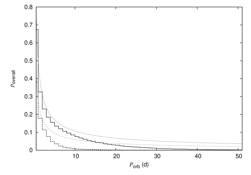
Figure 7: The overall expected WASP detection probability ($p_{\rm overall}$) as function of orbital period ($P_{\rm orb}$). Solid histogram is the case for a system with two identical stars, while the dashed histogram is that for a star with a small dark companion. The corresponding eclipsing probabilities discussed in Sect. 6.1 are given as grey lines for reference.

7 Discussion

7.1 Expected period distribution of Am binaries

The results from the radial velocity studies of Abt & Levy (1985) and Carquillat & Prieur (2007) can be used to predict the number and period distribution of eclipsing Am binaries. The combined sample comprises 151 Am stars, with 61 SB1s and 28 SB2s. This was binned onto 1-day bins, normalized by the total number of stars, to generate a period probability distribution for Am stars. Multiplying by the estimated WASP detection probability ($p_{\rm overall}$) obtained in Sect. 6 and by the number of stars in the WASP sample (1742), yields an estimate of the expected period distribution of eclipsing Am stars. In Figure 8 the WASP eclipsing Am star period distribution is compared to that predicted for the two identical stars and the dark companion cases. Since these represent the extrema of the probabilities, we also include the predicted distribution obtained using the ratio of SB1 and SB2 systems from the RV studies.

The number of eclipsing Am stars found by WASP does appear to be broadly consistent with the expected number of systems. We recall from Sect. 1 that the fraction of spectroscopic binaries is 60$\sim$70%. Thus, the eclipsing fraction appears to be similar, suggesting a significant fraction of Am stars might be single or have hard to detect companions. The period distribution is, however, slightly different, with a pronounced peak at shorter periods due to the inclusion of close binaries. The $v\sin i$ distributions of both Abt & Levy (1985) and Carquillat & Prieur (2007) are skewed toward lower values than the Renson & Manfroid (2009) sample. These radial velocity studies have preferentially avoided stars with high rotation, which accounts for the excess of short period systems found in the WASP sample. The distribution of Am-type spectroscopic binaries in the Renson & Manfroid (2009) catalogue (some 210 systems) shows a similar short orbital period excess, due to the inclusion of Am stars with a wide range of rotational velocities.

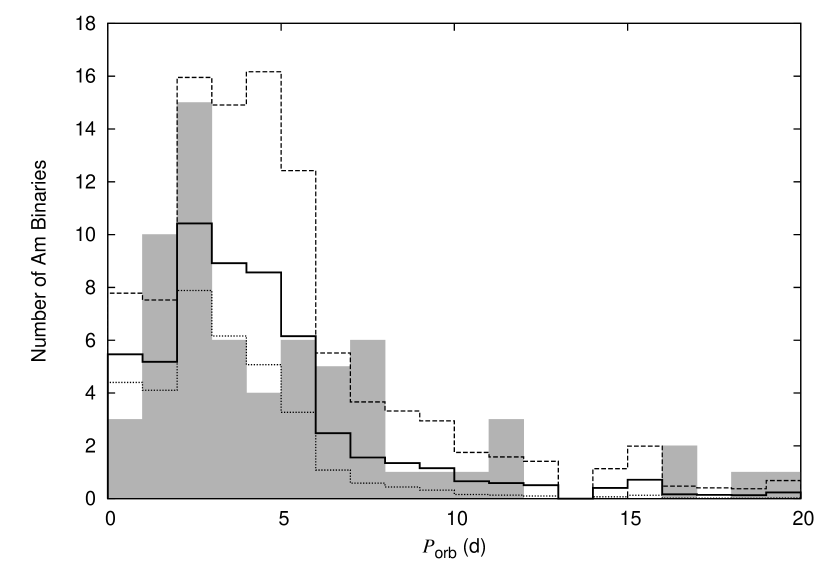
Figure 8: Period distribution of eclipsing Am star binaries. The WASP eclipsing Am star distribution is given as solid grey. The predicted period distribution based on the results of spectroscopic binaries are given as dashed-line for the two identical stars and dotted-line for the dark companion case. The thicker solid-line is that predicted based on the ratio of SB1 and SB2 systems.

7.2 Mass ratio distribution

Table 6: Results from jktebop fits to light curves (Detached systems only) and approximate stellar parameters, assuming primary is ${T_{\mathrm{eff}}}_{A}=7500$ K. See Text for details.

Renson	$\frac{R_{A}+R_{B}}{a}$	$R_{B}/R_{A}$	$i$	$e$	$J_{B}/J_{A}$	$P$	${T_{\mathrm{eff}}}_{B}$	$R_{A}$	$R_{B}$	$q$	$q$ (literature)
3750	0.307	0.111	89.95	0.00	0.00	1.2199	2000§	1.63	0.18	0.07	$<$0.003 (Collier Cameron et al., 2010)
4660	0.298	0.910	87.61	0.00	0.84	2.7807	7176	1.97	1.80	0.92	0.91 (Southworth et al., 2011)
6720	0.344	1.354	79.59	0.00	0.91	2.3832	7333	1.68	2.26	1.07
7310	0.161	0.601	86.37	0.00	0.50	6.6637	6322	2.20	1.32	0.71
7730	0.156	3.000	89.57	0.24	0.10	39.2827	4218	2.93	8.71	0.84	0.96 (Popper, 1988)
8215	0.105	0.940	86.43	0.00	0.44	8.7959	6126	1.38	1.29	0.77
9237	0.248	1.036	80.52	0.00	0.49	2.8562	6288	1.51	1.55	0.81
9318	0.148	0.472	85.89	0.06	0.72	11.1133	6901	3.24	1.52	0.71
9410	0.189	0.634	87.74	0.02	0.30	16.7873	5537	5.07	3.19	0.59	0.81† (Lucy & Sweeney, 1971)
10016	0.242	1.323	86.98	0.25	1.03	5.4309	7557	2.11	2.81	1.11
11100	0.165	0.397	85.07	0.00	0.36	4.0375	5818	1.79	0.71	0.61
11470	0.228	0.580	89.36	0.00	0.39	2.8721	5931	1.75	1.02	0.66
14850	0.215	0.272	83.02	0.00	0.08	3.9795	3925	2.43	0.66	0.30
15034	0.202	0.469	83.88	0.00	0.54	7.5392	6423	3.39	1.59	0.65
15190	0.174	0.439	82.60	0.00	0.02	5.1229	2952	1.97	0.86	0.21	0.33† (Carquillat et al., 2003)
15445	0.270	0.881	86.32	0.00	0.92	5.7606	7355	3.10	2.72	0.93
21400	0.106	0.513	86.63	0.00	0.04	7.7729	3435	1.49	0.77	0.29
22860	0.136	0.558	83.84	0.28	2.81	7.9006	9712	2.33	1.30	1.17
25020	0.188	0.081	89.10	0.00	0.00	6.6284	2000§	3.39	0.28	0.06
25070	0.185	0.500	85.60	0.14	0.91	6.7149	7323	2.85	1.42	0.79	1.00 (this work)
29290	0.314	0.977	79.45	0.00	0.95	3.2922	7406	2.30	2.23	0.98
30090	0.221	0.788	82.26	0.00	0.97	4.3486	7451	2.11	1.67	0.93
30110	0.148	0.162	84.55	0.00	0.09	4.3145	4108	1.92	0.31	0.37
30457	0.137	0.231	86.82	0.00	0.00	11.9420	2000§	3.20	0.74	0.08
30650	0.060	0.378	88.38	0.00	0.00	18.1210	2000§	1.53	0.58	0.09
35000	0.190	0.835	82.07	0.00	0.00	10.2861	2000§	2.69	2.26	0.13
36660	0.096	0.698	88.61	0.41	0.71	16.3653	6892	2.30	1.60	0.81	0.80 (this work)
37220	0.135	0.962	85.57	0.00	0.97	5.7931	7437	1.38	1.33	0.98
37610	0.240	1.455	85.50	0.00	1.28	3.2387	7974	1.38	2.02	1.19
38500	0.173	0.348	83.65	0.00	0.19	3.9938	4945	1.87	0.65	0.47
40350	0.156	0.272	88.22	0.00	0.00	7.0687	2000§	2.43	0.66	0.08
40910	0.132	1.114	87.17	0.05	1.05	11.1163	7594	2.03	2.23	1.05
42906	0.062	0.860	87.84	0.00	0.00	19.6987	2000§	1.23	1.06	0.12	0.98 (Carquillat et al., 2003)
44140	0.309	1.391	86.51	0.02	0.66	2.0598	6763	1.31	1.81	0.96	0.90 (Popper, 1970)
49380	0.161	0.355	85.06	0.11	0.57	5.0204	6508	2.14	0.76	0.68	0.83 (this work)
51506	0.322	0.119	80.30	0.12	0.17	1.9196	4787	2.69	0.32	0.46	0.12 (this work)
56310	0.285	1.108	84.26	0.00	0.88	2.6959	7258	1.68	1.85	0.99
58170	0.366	0.854	88.24	0.00	0.48	1.6047	6246	1.65	1.42	0.77	0.78 (Popper, 1968)
58256	0.271	0.378	81.63	0.00	0.41	2.9673	5983	2.50	0.95	0.59
59780	0.228	1.200	87.87	0.33	0.95	7.3514	7412	2.61	3.15	1.06	0.98 (Torres et al., 1999)

Without direct determinations of masses from spectroscopic studies, we can only make a rather crude estimate of the mass distribution of the eclipsing systems from their light curves and the jktebop fits. Since the bolometric correction for late-A stars is small, we can make the approximation that the ratio of bolometric surface brightnesses is given by the WASP bandpass surface brightness ratio ($J_{B}/J_{A}$). Thus the effective temperature of the secondary (${T_{\mathrm{eff}}}_{B}$) can be obtained from,

$${T_{\mathrm{eff}}}_{B}\approx{T_{\mathrm{eff}}}_{A}\times(J_{B}/J_{A})^{1/4},$$

where the effective temperature of the primary (${T_{\mathrm{eff}}}_{A}$) is assumed to be 7500 K. With initial mass estimates of $M_{A}$ = $M_{B}$ = 1.7, the known orbital period ($P_{\rm orb}$) and sum of the radii ($\frac{R_{A}+R_{B}}{a}$) from jktebop, we determine initial values for $R_{A}+R_{B}$. Using the ratio of the radii also from jktebop ($R_{B}/R_{A}$) we can determine individual values for $R_{A}$ and $R_{B}$. Next, the Torres et al. (2010) relations are used to determine stellar mass estimates, by varying $\log g$ so that radii obtained from Torres et al. (2010) agrees with that expected from the jktebop analysis. The procedure is iterated until there are no changes in parameters. The results are presented in Table 6, along with values for mass ratio ($q$) from spectroscopic analyses in the literature and those determined in Section 5. The average difference between our estimated $q$ values and the spectroscopic values is $-$0.11, but with an rms scatter of $\pm$0.25.

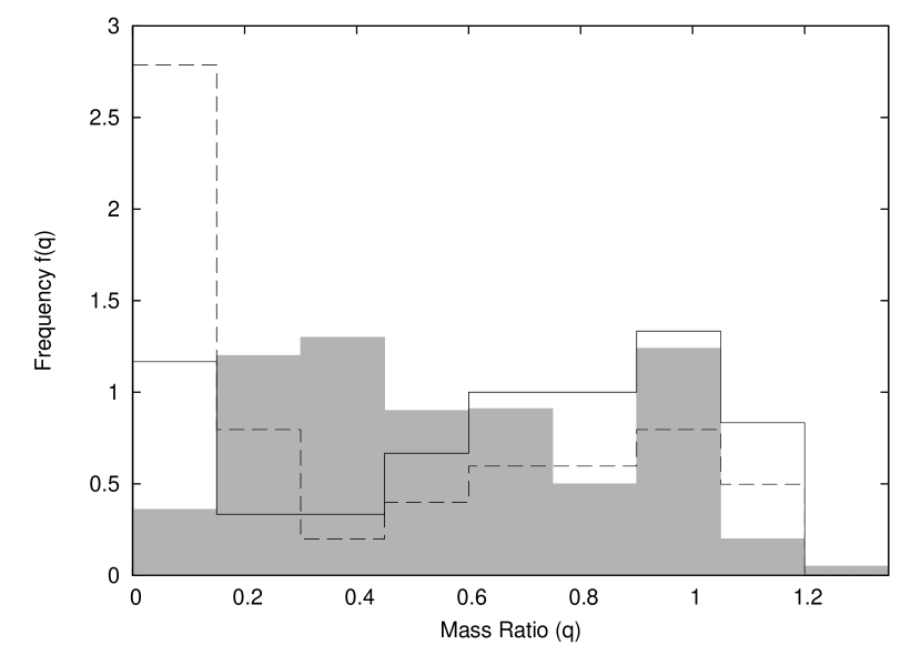
Figure 9: Mass ratio distribution for Am binary systems. The solid-line histogram is the distribution based on eclipsing binaries in the current work, while the solid grey histogram is that presented by Boffin (2010) based on the spectroscopic sample. The dashed histogram is the estimated eclipsing binary distribution after making allowance for the WASP detection probabilities.

As discussed in Sect. 6.1, eccentric systems may not always show two eclipses when both stars are similar. For example Renson 42906 (HD 151604; V916 Her) is an eccentric ($e=0.566$) system with mass ratio close to unity (Carquillat & Prieur, 2007), but the WASP data only shows one eclipse per orbit and value of $q=0.12$. Thus, these systems will appear to have anomalously low $q$ values, further adding to the uncertainty in the mass-ratio distribution.

Boffin (2010) concluded that the mass-ratio distribution showed hints of a double-peaked distribution, with peaks at $q\sim 0.3$ and $q\sim 1$. The mass-ratio distribution based on the estimated properties from the WASP light curves for detached systems is noticeably different (Fig. 9). The estimated WASP mass-ratio distribution shows a broad peak near unity, with a deficit around $q\simeq 0.3$. However, the WASP detection probability varies with companion size (Sect. 6.2). Assuming that companions with masses around 0.5 $M_{\sun}$ correspond to the transition between the two system scenarios discussed earlier, there would be an increase in the number of low $q$ systems relative to the high $q$ systems. The distribution would become flatter, similar to that found by Boffin (2010), who noted that a flat mass-ratio distribution also appeared to be a good fit. While there are genuinely low $q$ systems (e.g. Renson 3750), the apparent excess of such systems may not be real, since some of these may be pairs of similar stars with a true period equal to twice the assumed one (as noted with a dagger in Table 1). Hence, since our mass-ratio estimates are based on photometry alone, radial velocity studies are required to determine spectroscopic mass-ratios of the whole sample, before any firmer conclusions can be drawn.

8 Summary

A survey of 1742 Am stars using light curves from the SuperWASP project has found 70 eclipsing systems, of which 28 are previously unreported detections and 4 are suspected eclipsing systems. While this represents only 4% of the sample, after correction for eclipsing and WASP detection probabilities, the results are consistent with 60–70% incidence of spectroscopic binaries found from radial velocity studies (Abt & Levy, 1985; Carquillat & Prieur, 2007). This indicates that there is not a deficit of eclipsing Am binary systems, as suggested by Jaschek & Jaschek (1990).

Like the radial velocity studies, the WASP study suggests that around 30–40% of Am stars are either single or in very wide systems. The WASP survey is able to detect low-mass stellar and sub-stellar companions that were below the radial velocity studies’ detection limits. Thus, systems like HD 15082 (WASP-33) would not form part of the spectroscopic mass distribution. On the other hand, the WASP survey is unable to detect compact companions, such as white dwarfs, which would, if present, have been detected in the radial velocity studies. The average mass of a white dwarf is around 0.6 $M_{\sun}$ (Kleinman et al., 2013), corresponding to a $q$ of around 0.3$\sim$0.4. The only short-period system with a white dwarf companion in the Renson & Manfroid (2009) catalogue is HD 204188 (IK Peg) (Wonnacott et al., 1993), suggesting that such objects are relatively rare (Holberg et al., 2013).

Using jktebop fits to the WASP light curves, estimates of mass-ratios have been determined. The WASP mass-ratio distribution is consistent with that obtained from the spectroscopic studies (Boffin, 2010). However, if an approximate allowance is made for WASP detection probabilities there is a suggestion of an excess of low mass-ratio systems. While this could be explained by the presence of sub-stellar companions to Am stars, it is more likely that this is due to pairs of similar stars with true periods twice that assumed or the presence of eccentric systems exhibiting only one eclipse. Hence, radial velocity studies of the eclipsing systems found with WASP are required in order to fully explore the mass-ratio distribution of Am binary systems.