Non-maximal Tripartite Entanglement Degradation of Dirac and Scalar fields in Non-inertial frames

Abstract

The $\pi$-tangle is used to study the behavior of entanglement of a nonmaximal tripartite state of both Dirac and scalar fields in accelerated frame. For Dirac fields, the degree of degradation with acceleration of both one-tangle of accelerated observer and $\pi$-tangle, for the same initial entanglement, is different by just interchanging the values of probability amplitudes. A fraction of both one-tangles and the $\pi$-tangle always survives for any choice of acceleration and the degree of initial entanglement. For scalar field, the one-tangle of accelerated observer depends on the choice of values of probability amplitudes and it vanishes in the range of infinite acceleration, whereas for $\pi$-tangle this is not always true. The dependence of $\pi$-tangle on probability amplitudes varies with acceleration. In the lower range of acceleration, its behavior changes by switching between the values of probability amplitudes and for larger values of acceleration this dependence on probability amplitudes vanishes. Interestingly, unlike bipartite entanglement, the degradation of $\pi$-tangle against acceleration in the case of scalar fields is slower than for Dirac fields.

PACS: 03.65.Ud, 03.67.Mn, 04.70.Dy

Keywords: Tripartite entanglement, Noninertial frame

I Introduction

One of the potential resources for all kinds of quantum information tasks is entanglement. It is among the mostly investigated properties of many particles systems. Since the beginning of the birth of the fields of quantum information and quantum computation, it has been the pivot in different perspective to bloom up these fields to be matured for technological purposes Many1 . The recent development by mixing up the concepts of relativity theory with quantum information theory brought to fore the relative behavior of entanglement Alsing1 ; Alsing2 ; Alsing3 ; Fuentes . These studies show that entanglement not only depends on acceleration of the observer but also strongly depends on statistics. For practical application in most general scenario, it is essential to thoroughly investigate the behavior of entanglement and hence of different protocols (such as teleportation) of quantum information theory using different statistics in curved spacetime.

The observer dependent character of entanglement under various setup for different kinds of fields have been studied by a number of authors. For example, the entanglement between two modes of a free maximally entangled bosonic and fermionic pairs is studied in Alsing2 ; Alsing3 , between to modes of noninteracting massless scalar field is analyzed in Fuentes , between free modes of a free scalar field is investigated in Adesso . Similarly, the dynamics of tripartite entanglement under different situation for different fields has also been studied. For example, in Ref. Hwang the degradation of tripartite entanglement between the modes of free scalar field due to acceleration of the observer is investigated. All these studies are carried by taking single mode approximation. The behavior of entanglement in accelerated frame beyond the single mode approximation is studied in Ref. Bruchi . The effect of decoherence on the behavior of entanglement in accelerated frame is studied in Ref. Salman . All these and many other related works show that entanglement in the initial state is degraded when observed from the frame of an accelerated observer.

On the other hand, there are studies which show, counter intuitively, that the Unruh effect not only degrade entanglement shared between an inertial and an accelerated observer but also amplify it. Ref. Montero studies such entanglement amplification for a particular family of states for scalar and Grassman scalar fields beyond the single mode approximation. A similar entanglement amplification is reported for fermionic system in Ref. Kown . There are a number of other good papers on the dynamics of entanglement in accelerated frames which can be found in the list Pan2 .

It is well known that considering correlations between the modes of stationary observer with both particle and anti-particle modes in the two causally disconnected regions in the Rindler spacetime provides a broad view for quantum communications tasks. Such considerations enable the stationary observer to setup communication with either of the two disconnected regions or with both at the same time Martin2 . This is possible by considering the formalism of quantum communication in the limit of beyond single mode approximation Bruchi . In the same work it is shown that the single mode approximation holds for some family of states under appropriate constraints. On the other hand, it has also been suggested that the single mode approximation is optimal for quantum communication between the stationary observer and the accelerated observer Hosler . For the purpose of this paper we will use the later approach.

In this paper, we investigate the dependence of the behavior of a nonmaximal tripartite entanglement of both Dirac and scalar fields on the acceleration of the observer frame and on the entanglement parameter that describes the degree of entanglement in the initial state. We show that the degradation of entanglement with acceleration not only depends on the degree of initial entanglement but also depends on the individual values of the normalizing probability amplitudes of the initial state. We consider three observers ($i=A,B,C$), Alice Bob and Charlie, in Minkowski space such that each of them observes only one part of the following nonmaximal initial tripartite entangled state

$$\left|\psi_{\omega_{A},\omega_{B},\omega_{C}}\right\rangle=\alpha\left|0_{\omega_{A}}\right\rangle_{A}\left|0_{\omega_{B}}\right\rangle_{B}\left|0_{\omega_{C}}\right\rangle_{C}+\sqrt{1-\alpha^{2}}\left|1_{\omega_{A}}\right\rangle_{A}\left|1_{\omega_{B}}\right\rangle_{B}\left|1_{\omega_{C}}\right\rangle_{C},$$ (1)

where $\left|m_{\omega_{i}}\right\rangle$ for $m\in(0,1)$ are the Minkowski vacuum and first excited states with modes specified by the subscript $\omega_{i}$ and $\alpha$ is a parameter that specify the degree of entanglement in the initial state. Under the single mode approximation Bruchi $\omega_{A}\sim\omega_{B}\sim\omega_{C}=\omega,$ we can write $\left|m_{\omega_{i}}\right\rangle=\left|m\right\rangle_{i}$.

Instead of being all the time in an inertial frame, if the frame of one of the observers, say Charlie, suddenly gets some uniform acceleration $a$, then, the Minkowski vacuum and excited states change from the perspective of the accelerated observer. The appropriate coordinates for the viewpoint of an accelerated observer are Rindler coordinates AsPach ; Martin ; Bruchi ; Brown2 . The Rindler spacetime for an accelerated observer splits into two regions, $\mathrm{I}$ (right) and $\mathrm{II}$ (left), that are separated by Rindler horizon and thus are causally disconnected from each other. The Rindler coordinates $(\tau,\xi)$ in region $\mathrm{I}$ are defined in terms of the Minkowski coordinates $(t,x)$ as follows

$$t=\frac{1}{a}e^{a\xi}\sinh(a\tau),\qquad x=\frac{1}{a}e^{a\xi}\cosh(a\tau).$$ (2)

An exact similar transformation holds between the coordinates for the Rindler region $\mathrm{II}$, however, each coordinate differ by an overall minus sign. These new coordinates allow us to perform a Bogoliubov transformation between the Minkowski modes of a field and Rindler modes. The Rindler modes in the two Rindler regions form a complete basis in terms of which the Minkowski modes can be expanded. Thus any state in Minkowski space can be represented in Rindler basis as well. However, an accelerated observer in Rindler region $\mathrm{I}$ has no access to information in Rindler region $\mathrm{II}$. The degree of entanglement of modes in each Rindler region with the modes of inertial observers has its own dynamics. To study the behavior of entanglement in one region, being inaccessible, the modes in other region becomes irrelevant and thus need to be trace out.

The Minkowski annihilation operator of an arbitrary frequency, observed by Alice, is related to the two Rindler regions’ operators of frequency, observed by Charlie, more directly through an intermediate set of modes called Unruh modes Bruchi . The Unruh modes analytically extend the Rindler region$I$ modes to region $II$ and the region$II$ modes to region $I$. Since the Unruh modes exist over all Minkowski space, they share the same vacuum as the Minkowski annihilation operators. An arbitrary Unruh mode for a give acceleration is given by

$$C_{\omega}=q_{L}C_{\omega,L}+q_{R}C_{\omega,R},$$ (3)

where $q_{L}$ and $q_{R}$ are complex numbers satisfying the relation $\left|q_{L}\right|^{2}+\left|q_{R}\right|^{2}=1$ and the appropriate relations for the left and right regions’ operators are given by Bruchi

$$C_{\omega,R} =\cosh r_{\omega}a_{\omega,I}-\sinh r_{\omega}a_{\omega,II}^{{\dagger}},$$

$$C_{\omega,L} =\cosh r_{\omega}a_{\omega,II}-\sinh r_{\omega}a_{\omega,I}^{{\dagger}},$$ (4)

where $a$, $a^{{\dagger}}$ are Rindler particle operators of scalar field in the two regions. For Grassman case, the transformation relations are given by

$$C_{\omega,R} =\cos r_{\omega}c_{\omega,I}-\sinh r_{\omega}d_{\omega,II}^{{\dagger}},$$

$$C_{\omega,L} =\cos r_{\omega}c_{\omega,II}-\sinh r_{\omega}d_{\omega,I}^{{\dagger}},$$ (5)

where $c$, $c^{{\dagger}}$ and $d$, $d^{{\dagger}}$ are respectively Rindler particle and antiparticle operators. The dimensionless parameter $r_{\omega}$ appears in these equations is discussed below. For the purpose of this paper, in order to recover single mode approximation we will set $q_{R}=1$ and $q_{L}=0$.

From the viewpoint of accelerated observer, the Minkowski vacuum and excited states of the Dirac field are found to be, respectively, given by Alsing3 .

$$\left|0\right\rangle_{M}=\cos r\left|0\right\rangle_{I}\left|0\right\rangle_{II}+\sin r\left|1\right\rangle_{I}\left|1\right\rangle_{II},$$ (6)

$$\left|1\right\rangle_{M}=\left|1\right\rangle_{I}\left|0\right\rangle_{II}.$$ (7)

Similarly, for scalar field the Minkowski vacuum and excited states are given by

$$\left|0\right\rangle_{M}=\frac{1}{\cosh r}{\displaystyle\sum\limits_{n=0}^{\infty}}\tanh^{n}r\left|n\right\rangle_{I}\left|n\right\rangle_{II},$$ (8)

$$\left|1\right\rangle_{M}=\frac{1}{\cosh^{2}r}{\displaystyle\sum\limits_{n=0}^{\infty}}\sqrt{n+1}\tanh^{n}r\left|n+1\right\rangle_{I}\left|n\right\rangle_{II}.$$ (9)

In the above equations, $\left|\cdot\right\rangle_{I}$ and $\left|\cdot\right\rangle_{II}$ are Rindler modes in the two causally disconnected Rindler regions, $\left|n\right\rangle$ represents number states and $r$ is a dimensionless parameter that depends on acceleration of the moving observer and modes frequency. For Dirac field, it is given by $\cos r=(1+e^{-2\pi\omega c/a})^{-1/2}$ such that $0\leq r\leq\pi/4$ for $0\leq a\leq\infty$ and for scalar field, it is defined as $\cosh r=(1-e^{-2\pi\omega c/a})^{-1/2}$ such that $0\leq r\leq\infty$ for $0\leq a\leq\infty$. It is important to note that almost all the previous studies have been focused on investigating the influence of parameter $r$, as a function of acceleration of the moving frame by fixing the Rindler frequency, on the degree of entanglement present in the initial state. Such analysis lead to the measurement of entanglement in a family of states, all of which share the same Rindler frequency as seen by an observer with different acceleration. However, the effect of parameter $r$ on entanglement can also, alternatively, be interpreted by considering a family of states with different Rindler frequencies watched by the same observer traveling with fixed acceleration Bruschi2 .

II Quantification of Tripartite entanglement

In literature, a number of different criterion for quantifying tripartite entanglement exist. However, the most popular among them are the residual three tangle Coffman and $\pi$-tangle Fan ; Vidal . Other measurements for tripartite entanglement include realignment criterion Rudolph ; Kia and linear contraction Horodocki . The realignment and linear contraction criterion are comparatively easy in calculation and are strong criteria for entanglement measurement. However, these criterion has some limitations and do not detect the entanglement of all states.

The three tangle is another good quantifier for the entanglement of tripartite states. This is polynomial invariant Verstraete ; Leifer and it needs an optimal decomposition of a mixed density matrix. In general, the optimal decomposition is a tough enough task except in a few rare cases Lohmayer . On the other hand, the $\pi$-tangle for a tripartite state $|\psi\rangle_{ABC}$ is given by

$$\pi_{ABC}=\frac{1}{3}(\pi_{A}+\pi_{B}+\pi_{C}),$$ (10)

where $\pi_{A}$ is called residual entanglement and is given by

$$\pi_{A}=\mathcal{N}_{A(BC)}^{2}-\mathcal{N}_{AB}^{2}-\mathcal{N}_{AC}^{2}.$$ (11)

The other two residual tangles ($\pi_{B},\pi_{C}$) are defined in a similar way. In Eq. (11), $\mathcal{N}_{AB}(\mathcal{N}_{AC})$ is a two-tangle and is given as the negativity of mixed density matrix $\rho_{AB}=Tr_{C}|\psi\rangle_{ABC}\langle\psi|$ $(\rho_{AC}=Tr_{B}|\psi\rangle_{ABC}\langle\psi|)$. The $\mathcal{N}_{A(BC)}$ is a one-tangle and is defined as $\mathcal{N}_{A(BC)}=\left\|\rho_{ABC}^{T_{A}}\right\|-1$, where $\left\|O\right\|=\mathrm{tr}\sqrt{OO^{{\dagger}}}$ stands for the trace norm of an operator $O$ and $\rho_{ABC}^{T_{A}}$ is the partial transposition of the density matrix over qubit $A$. The one-tangle and the two-tangles satisfy the following Coffman-Kundu-Wootters (CKW) monogamously inequality relation Coffman .

$$\mathcal{N}_{A(BC)}^{2}\geq\mathcal{N}_{AB}^{2}+\mathcal{N}_{AC}^{2}.$$ (12)

In this paper we use the $\pi$-tangle to observe the behavior of entanglement of the state given in Eq. (1), as a function of acceleration of the observer and the entanglement parameter $\alpha$.

III Nonmaximal tripartite entanglement

III.1 Fermionic Entanglement

To study the influence of acceleration parameter $r$ and the entanglement parameter $\alpha$ on the entanglement between modes of Dirac field, we substitute Eqs.(6) and (7) for Charlie part in Eq.(1) and rewrite it in terms of Minkowski modes for Alice and Bob and Rindler modes for Charlie as follow

$$\left|\psi_{ABCI,II}\right\rangle=\alpha(\cos r\text{ }\left|0000\right\rangle+\sin r\text{ }\left|0011\right\rangle)+\sqrt{1-\alpha^{2}}\left|1110\right\rangle,$$ (13)

where $\left|abcd\right\rangle=\left|a\right\rangle_{A}\left|b\right\rangle_{B}\left|c\right\rangle_{CI}\left|d\right\rangle_{CII}$. Note that for the purpose of writing ease, we have also dropped the frequency in the subscript of each ket. Being inaccessible to Charlie in Rindler region I, the modes in Rindler region II must be trace out for investigating the behavior of entanglement between the modes of inertial observers and the modes of Charlie in region I. So, tracing out over the forth qubit, leaves the following mixed density matrix between the modes of Alice, Bob and Charlie,

$$\rho_{ABC} =\alpha^{2}\cos^{2}r\left|000\right\rangle\left\langle 000\right|+\alpha\sqrt{1-\alpha^{2}}\cos r(\left|000\right\rangle\left\langle 111\right|+\left|111\right\rangle\left\langle 000\right|)$$

$$+\alpha^{2}\sin^{2}r\left|001\right\rangle\left\langle 001\right|+(1-\alpha^{2})\left|111\right\rangle\left\langle 111\right|.$$ (14)

Taking partial transpose over each qubit in sequence and using the definition of one-tangle, the three one-tangles can straightforwardly be calculated, which are given by

$$\mathcal{N}_{A(BC)}=\mathcal{N}_{B(AC)}=2\alpha\sqrt{1-\alpha^{2}}\cos r.$$ (15)

$$\mathcal{N}_{C(AB)}=\alpha\sqrt{1-\alpha^{2}}\cos r-\alpha^{2}\sin^{2}r+\alpha\sqrt{(1-\alpha^{2})\cos^{2}r+\alpha^{2}\sin^{4}r}.$$ (16)

Note that $\mathcal{N}_{A(BC)}=\mathcal{N}_{B(AC)}$ shows that the two subsystems of inertial frames are symmetrical for any values of the parameters $\alpha$ and $r$. It can easily be checked that all the one-tangles reduce to $1$ for a maximally entangled initial state with no acceleration, which is a verification of the result obtained in the rest frames both for Dirac and Scalar fields Hwang ; Wang . To have a better understanding of the influence of the two parameters, we plot the one-tangles for different values of $\alpha$ against $r$ in Fig. $1$(a, b).

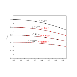
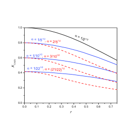
Figure 1: (Color Online) The one-tangles (a) $\mathcal{N}_{A(BC)}$ and (b) $\mathcal{N}_{C(AB)}$ of fermionic modes as a function of the acceleration parameter $r$ for different values of the entanglement parameter $\alpha$ and its normalized partners $\sqrt{1-\alpha^{2}}$. The black solid line corresponds to maximally entangled initial state. The blue solid lines from top to bottom correspond to $\left|\alpha\right|=\frac{1}{\sqrt{5}}$, $\frac{1}{\sqrt{10}}$, $\frac{1}{\sqrt{22}}$ and red dashed lines from top to bottom correspond to $\left|\alpha\right|=\frac{2}{\sqrt{5}}$, $\frac{3}{\sqrt{10}}$, $\sqrt{\frac{21}{22}}$.

Figure (1a) shows the behavior of $\mathcal{N}_{A(BC)}=\mathcal{N}_{B(AC)}$ and figure (1b) is the plot of $\mathcal{N}_{C(AB)}$. A comparison of the two figures shows that for maximal entangled initial state ($\alpha=1/\sqrt{2}$) and hence for all other values of $\alpha$, the $\mathcal{N}_{C(AB)}$ falls off rapidly with increasing acceleration as compared to $\mathcal{N}_{A(BC)}$. However, the most interesting feature of the two figures is the different response of the one-tangles to the parameter $\alpha$. The behavior of $\mathcal{N}_{A(BC)}$ ($\mathcal{N}_{B(AC)}$) is unchanged by interchanging the values of $\alpha$ and its normalizing partner $\sqrt{1-\alpha^{2}}$. On the other hand, $\mathcal{N}_{C(AB)}$ degrades along different trajectories by switching the values of $\alpha$ and $\sqrt{1-\alpha^{2}}$. This shows an inequivalence of the quantization for Dirac field in the Minkowski and Rindler coordinates. Regardless of the amount of acceleration, there is always some amount of one-tangle left for each subsystem, which ensures the application of entanglement based quantum information tasks between relatively accelerated parties. The values chosen for entanglement parameter $\alpha$ and its normalizing partner $\sqrt{1-\alpha^{2}}$ in figure (1) are $\frac{1}{\sqrt{2}},\frac{1}{\sqrt{5}},\frac{2}{\sqrt{5}},\frac{1}{\sqrt{10}},\frac{3}{\sqrt{10}},\frac{1}{\sqrt{22}},\sqrt{\frac{21}{22}}$.

The next step is to evaluate the two-tangles. According to its definition, we need to take partial trace over each qubit one by one. So, taking partial trace of the final density matrix of Eq. (14) over Alice’s qubit or Bob’s qubit leads to the following mixed density matrix

$$\rho_{AC(BC)}=\rho_{ABC}^{T_{B(A)}}=\alpha^{2}\cos^{2}r\left|00\right\rangle\left\langle 00\right|+\alpha^{2}\sin^{2}r\left|01\right\rangle\left\langle 01\right|+(1-\alpha^{2})\left|11\right\rangle\left\langle 11\right|.$$ (17)

Note that this matrix is diagonal and the partial transpose over either qubit leaves it unchanged. Similarly, the reduced density matrix $\rho_{AB}$, which is obtained by taking partial trace over the Charlie qubit, is diagonal. Using the definition of negativity, one can easily show that there exists no entanglement between any of these subsystems of the tripartite state $\rho_{ABC}$. Since this result is valid for a maximally entangled GHZ state in inertial frame, it shows that the entanglement behavior of subsystems is independent from the status of the observer and from the degree of initial entanglement in the state. Also, the zero value of all the two-tangles verify the validity of the CKW inequality.

Since we now know all the one-tangles and all the two-tangles of the tripartite state $\rho_{ABC}$, we can find the $\pi$-tangle. As all the two-tangles are zero, using Eq. (10), it simply becomes

$$\pi_{ABC} =\frac{1}{3}(\mathcal{N}_{A(BC)}^{2}+\mathcal{N}_{B(AC)}^{2}+\mathcal{N}_{C(AB)}^{2})$$

$$=\frac{\alpha^{2}}{3}[\left(\sqrt{(1-\alpha^{2})}\cos^{2}r-\alpha\sin^{2}r+\sqrt{(1-\alpha^{2})\cos^{2}r+\alpha^{2}\sin^{4}r}\right)^{2}$$

$$+8(1-\alpha^{2})\cos^{2}r].$$ (18)

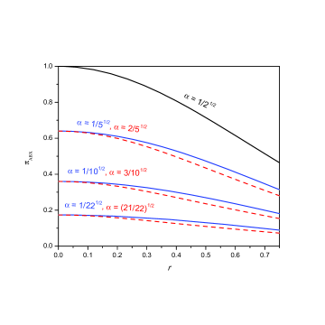
Figure 2: (Color Online) The $\pi$-tangle of fermionic modes as a function of acceleration parameter $r$ for different values of entanglement parameter $\alpha$ and its normalized partner $\sqrt{1-\alpha^{2}}$. The black solid line corresponds to maximally entangled initial state. The blue solid lines from top to bottom correspond to $\left|\alpha\right|=\frac{1}{\sqrt{5}}$, $\frac{1}{\sqrt{10}}$, $\frac{1}{\sqrt{22}}$ and the red dashed lines from top to bottom correspond to $\left|\alpha\right|=\frac{2}{\sqrt{5}}$, $\frac{3}{\sqrt{10}}$, $\sqrt{\frac{21}{22}}$.

It is straightforward to verify that for inertial frame and maximally entangled initial state the result of Eq. (18) is $1$. To have a more close look on how it is effected by the parameters $\alpha$ and $r$, we plot it against the parameter $r$ for different values of the entanglement parameter $\alpha$ in Fig. $2$. Like the one-tangles, the $\pi$-tangle exhibit a similar behavior in response to $\alpha$. Here the solid black line represents the behavior of $\pi$-tangle against $r$ when the initial state is maximally entangled. It can be seen that for the same entanglement in the initial state, interchanging the values of $\alpha$ and its normalizing partner $\sqrt{1-\alpha^{2}}$ leads to two different degradation curves for $\pi$-tangle against the acceleration parameter $r$. This degradation behavior of $\pi$-tangle along two different curves is similar to the degradation of logarithmic negativity for bipartite fermionic entangled states Pan . It is interesting to note that the loss of entanglement against the acceleration parameter is rapid for states of stronger initial entanglement. Nevertheless, the rate of degradation of $\pi$-tangle is slower than the logarithmic negativity for bipartite fermionic states.

III.2 Bosonic Entanglement

To study the behavior of entanglement of nonmaximal initial state of scalar field, we follow the same procedure as we used to investigate the dynamics of entanglement of Dirac Field. For Charlie in noninertial frame, the nonmaximal entangled initial state of Eq. (1) can be rewritten in terms of Minkowski modes for Alice and Bob and Rindler modes of Fock space for Charlie by using Eqs. (8) and (9) as follow

$$\left|\varphi_{ABCI,II}\right\rangle=\frac{1}{\cosh r}{\displaystyle\sum\limits_{n=0}^{\infty}}\tanh^{n}r\left[\alpha\left|00nn\right\rangle+\frac{\sqrt{(n+1)(1-\alpha^{2})}}{\cosh r}\left|11n+1n\right\rangle\right],$$ (19)

where, again, the kets $\left|abcd\right\rangle=\left|a\right\rangle_{A}\left|b\right\rangle_{B}\left|c\right\rangle_{CI}\left|d\right\rangle_{CII}$. In response to acceleration, for the behavior of entanglement between the modes of inertial observers and the modes of Charlie in region I, the inaccessible modes in region II must be trace out. Tracing out over those modes, leaves the following mixed density matrix

$$\varrho_{ABC} =\alpha^{2}\left|00\right\rangle\left\langle 00\right|\otimes M_{n,n}+(1-\alpha^{2})\left|11\right\rangle\left\langle 11\right|\otimes M_{n+1,n+1}+$$

$$\alpha\sqrt{(1-\alpha^{2})}(\left|11\right\rangle\left\langle 00\right|\otimes M_{n+1,n}+\left|00\right\rangle\left\langle 11\right|\otimes M_{n,n+1}),$$ (20)

where

$$M_{n,n} =\frac{1}{\cosh^{2}r}{\displaystyle\sum\limits_{n=0}^{\infty}}\tanh^{2n}r\left|n\right\rangle\left\langle n\right|,$$

$$M_{n,n+1} =\frac{1}{\cosh^{3}r}{\displaystyle\sum\limits_{n=0}^{\infty}}\sqrt{(n+1)}\tanh^{2n}r\left|n\right\rangle\left\langle n+1\right|,$$

$$M_{n+1,n} =\frac{1}{\cosh^{3}r}{\displaystyle\sum\limits_{n=0}^{\infty}}\sqrt{(n+1)}\tanh^{2n}r\left|n+1\right\rangle\left\langle n\right|,$$

$$M_{n+1,n+1} =\frac{1}{\cosh^{4}r}{\displaystyle\sum\limits_{n=0}^{\infty}}(n+1)\tanh^{2n}r\left|n+1\right\rangle\left\langle n+1\right|.$$ (21)

The three one-tangles can be computed, as before, by taking partial transpose of the density matrix of Eq. (20) with respect to each qubit one by one. It is easy to prove that the two one-tangles which are obtained from partial transposed of the qubits of inertial observers are equal and is given by

$$\mathcal{N}_{A(BC)}=\mathcal{N}_{B(AC)}=\frac{2\alpha\sqrt{1-\alpha^{2}}}{\cosh^{3}r}\sum_{n=0}^{\infty}\sqrt{(n+1)}\tanh^{2n}r.$$ (22)

We can write this relation into another more compact form as follow

$$\mathcal{N}_{A(BC)}=\frac{2\alpha\sqrt{1-\alpha^{2}}}{\cosh r\sinh^{2}r}\mathbf{Li}_{-\frac{1}{2}}(\tanh^{2}r),$$ (23)

where we have used the following identities

$$\sum_{n=0}^{\infty}(n+1)\tanh^{2n}r =\cosh^{4}r$$

$$\sum_{n=0}^{\infty}\tanh^{2n}r =\cosh^{2}r.$$ (24)

The function $\mathbf{Li}_{n}(x)$ in Eq. (23) is a polylogarithm function and is given by

$$\mathbf{Li}_{n}(x)\equiv\sum_{k=1}^{\infty}\frac{x^{k}}{k^{n}}=\frac{x}{1^{n}}+\frac{x^{2}}{2^{n}}+\frac{x^{3}}{3^{n}}+...$$ (25)

To compute the one tangle $\mathcal{N}_{C(AB)}$, first we find $\varrho_{ABC}^{T_{C}}$ from Eq.(20) and then we construct $(\varrho_{ABC}^{T_{C}})(\varrho_{ABC}^{T_{C}})^{{\dagger}}$, whose explicit expression is given by

$$(\varrho_{ABC}^{T_{C}})(\varrho_{ABC}^{T_{C}})^{{\dagger}} =\sum_{n=0}^{\infty}\frac{\tanh^{4n}r}{\cosh^{4}r}[(\alpha^{4}+\frac{n\alpha^{2}(1-\alpha^{2})\cosh^{2}r}{\sinh^{4}r})\left|00n\right\rangle\left\langle 00n\right|+\frac{\alpha((n+1)(1-\alpha^{2})x)^{\frac{1}{2}}}{\cosh r}$$

$$(\alpha^{2}\tanh^{2}r+\frac{n(1-\alpha^{2})}{\sinh^{2}r})\{\left|00n+1\right\rangle\left\langle 11n\right|+\left|11n\right\rangle\left\langle 00n+1\right|\}$$

$$+(\frac{\alpha^{2}(1-\alpha^{2})(n+1)}{\cosh^{2}r}+\frac{n^{2}(1-\alpha^{2})^{2}}{\sinh^{4}r})\left|11n\right\rangle\left\langle 11n\right|].$$ (26)

The nonvanishing eigenvalues Eq. (26) are

$$\left(\frac{\alpha^{4}}{\cosh^{4}r},\Lambda_{n}^{\pm},\text{ \ \ }(n=0,1,2,3,...)\right),$$ (27)

where

$$\Lambda_{n}^{\pm}=\frac{1}{2}(\xi\pm\sqrt{\eta+\mu}),$$ (28)

and

$$\xi =\frac{\tanh^{4n}r}{\cosh^{4}r}\left(\frac{n^{2}(1-\alpha^{2})^{2}}{\sinh^{4}r}+\frac{2\alpha^{2}(1-\alpha^{2})(n+1)}{\cosh^{2}r}+\alpha^{4}\tanh^{4}r\right),$$

$$\mu =\frac{4\alpha^{2}(1-\alpha^{2})(n+1)}{\cosh^{2}r}\frac{\tanh^{8n}r}{\cosh^{8}r}\left(\frac{n(1-\alpha^{2})}{\sinh^{2}r}+\alpha^{2}\tanh^{2}r\right)^{2},$$

$$\eta =\frac{\tanh^{8n}r}{\cosh^{8}r}\left(\frac{n^{2}(1-\alpha^{2})^{2}}{\sinh^{4}r}-\alpha^{4}\tanh^{4}r\right)^{2}.$$ (29)

Using the definition of one-tangle, one can obtain $\mathcal{N}_{C(AB)}$ whose explicit expression is by

$$\mathcal{N}_{C(AB)}=-1+\frac{\alpha^{2}}{\cosh^{2}r}+\sum_{n=0}^{\infty}\frac{\tanh^{2n}r}{\cosh^{2}r}\sqrt{\frac{n^{2}(1-\alpha^{2})^{2}}{\sinh^{4}r}+\frac{2\alpha^{2}(1-\alpha^{2})(n+2)}{\cosh^{2}r}+\alpha^{4}\tanh^{4}r}$$ (30)

It is easy to check that the one-tangles results into $1$ for $r=0$ and maximally entangled initial state.

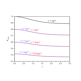
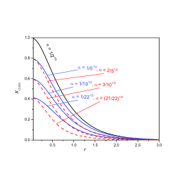
Figure 3: (Color Online)The one-tangle (a) $\mathcal{N}_{A(BC)}$ and (b) $\mathcal{N}_{C(AB)}$ of bosonic field as a function of the acceleration parameter $r$ for different values of entanglement parameter $\alpha$ and its normalized partners $\sqrt{1-\alpha^{2}}$. The black solid line corresponds to maximally entangled initial state. The blue solid lines from top to bottom correspond to $\left|\alpha\right|=\frac{1}{\sqrt{5}}$, $\frac{1}{\sqrt{10}}$, $\frac{1}{\sqrt{22}}$ and the red dashed lines from top to bottom correspond to $\left|\alpha\right|=\frac{2}{\sqrt{5}}$, $\frac{3}{\sqrt{10}}$, $\sqrt{\frac{21}{22}}$.

The dependence of one-tangles on $r$ and $\alpha$, in this case, is shown in figure ($3$). As can be seen, the one-tangles are strongly effected by the parameters $\alpha$ and $r$. However, as before, switching between the values of $\alpha$ and its normalizing partner $\sqrt{1-\alpha^{2}}$ does not effect the behavior of one-tangle, corresponds to an inertial observer, against $r$ as shown in figure ($3a$). Unlike the fermionic case, the loss in one-tangle $\mathcal{N}_{A(BC)}$ with acceleration is not uniform through the whole range of $r$. In fermionic case, it is monotonic strictly decreasing whereas in bosonic case, it is only monotonic decreasing, however, it never vanishes completely. On the other hand, figure ($3b$) shows that, like the fermionic case, the one-tangle $\mathcal{N}_{C(AB)}$ degrades along different curves against $r$ by interchanging the values of $\alpha$ and $\sqrt{1-\alpha^{2}}$, however, it vanishes , regardless of the value of $\alpha$, in the asymptotic limit. The loss in $\mathcal{N}_{C(AB)}$ against $r$ depends on the degree of entanglement in the initial state, it is faster when the entanglement is stronger initially.

Similar to the case of Dirac field, we have verified that all the two tangles for scalar field are also zero, that is,

$$\mathcal{N}_{AB}=\mathcal{N}_{AC}=\mathcal{N}_{BC}=0.$$ (31)

This verifies that CKW inequality also holds for scalar field. Again, the zero values of all the two tangles make it easier to find the $\pi$-tangle. Instead of writing its explicit relation, which is lengthy enough, we want to show its behavior by plotting it against $r$ for different values of $\alpha$ in figure ($4$).

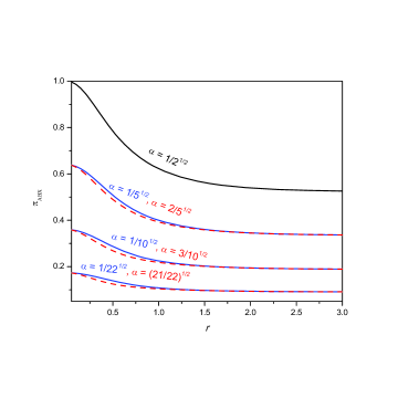
Figure 4: (Color Online) The $\pi$-tangle of bosonic field as a function of acceleration parameter $r$ for different values of entanglement parameter $\alpha$ and its normalized partners $\sqrt{1-\alpha^{2}}$. The black solid line corresponds to maximally entangled initial state. The blue solid lines from top to bottom correspond to $\left|\alpha\right|=\frac{1}{\sqrt{5}}$, $\frac{1}{\sqrt{10}}$, $\frac{1}{\sqrt{22}}$ and the red dashed lines from top to bottom correspond to $\left|\alpha\right|=\frac{2}{\sqrt{5}}$, $\frac{3}{\sqrt{10}}$, $\sqrt{\frac{21}{22}}$.

The figure shows that in the range of larger acceleration, the loss of $\pi$-tangle depends only on the initial value of the degree of entanglement. This shows that the response of $\pi$-tangle to $r$ is different from logarithmic negativity for bipartite state because the latter does depend on the choice of values of $\alpha$ and $\sqrt{1-\alpha^{2}}$. However, for smaller values of acceleration, it does degrades, like the logarithmic negativity for bipartite states, along two different trajectories by interchanging the values of $\alpha$ and $\sqrt{1-\alpha^{2}}$. For every value of initial entanglement, it has a nonvanishing value at infinite acceleration. The notable feature of figure ($4$) is that, unlike bipartite entanglement, the tripartite entanglement for scalar field degrades slowly with acceleration than for Dirac field and it always remains finite in the limit of larger values of $r$.

IV Summary

In this paper, we have investigated the entanglement behavior of nonmaximal tripartite quantum states in both fermionic and bosonic systems when one of the parties is traveling with a uniform acceleration. Rindler coordinates are used for the accelerating party. The behavior of entanglement against the acceleration parameter and the initial entanglement parameter is quantified using $\pi$-tangle.

It is shown that the entanglement in tripartite GHZ states does not only depend on the acceleration and initial entanglement in the states but also depends, for the same initial entanglement, on the probability amplitudes of the bases vectors. The one-tangles corresponding to accelerated observer, in both bosonic and fermionic cases, strongly depends on the entanglement parameter $\alpha$. However, in the fermionic case, it never vanishes for any values of $\alpha$ even in the limit of infinite acceleration. Whereas in bosonic case, regardless of the value of $\alpha$, it vanishes in the range of infinite acceleration. The two-tangles, in both cases, are always zero, which means that the acceleration and the degree of initial entanglement do not affect the entanglement behavior of any of the sub-bipartite systems.

The response of $\pi$-tangle to $r$ and $\alpha$ in the two cases is considerably different. In fermionic case, for the same initial entanglement, it strongly depends on the values of $\alpha$ and $\sqrt{1-\alpha^{2}}$. The difference in degradation against $r$, by interchanging the values of probability amplitudes, increases with increasing acceleration. However, some fraction of $\pi$-tangle always survives for all values of $\alpha$ even in the limit of infinite acceleration. For bosonic case, in the range of large values of $r$, the $\pi$-tangle just depends on the of initial entanglement,. However, for small values of $r$, its degradation is different by interchanging the values of probability amplitudes. Amazingly unlike bipartite entanglement, the $\pi$-tangle in fermionic case degrades quickly against the acceleration as compared to bosonic case. The survival of tripartite entanglement may be used to perform different quantum information task in situations where execution of such task through bipartite entanglement fails, for example, between inside and outside of the black hole.

References

- (1) D. Bouwmeester, A. Ekert, and A. Zeilinger, “The Physics of Quantum Information” (Springer-Verlag, Berlin, 2000); A. Peres and D. R. Terno, Rev. Mod. Phys.76, 93 (2004); C. H. Bennett, et al, Phys. Rev. Lett. 70, 1895 (1993); S. F. Huegla, M. B. Plenio, and J. A. Vaccaro, Phys. Rev. A 65, 042316 (2002); J. L. Dodd, M. A. Nielsen, M. J. Bremner, and R. T. Thew, Phys. Rev. A 65, 040301 (2002).
- (2) P. M. Alsing, David McMahon and G J Milburn, J. Opt. B: Quantum Semiclass. Opt. 6, 834 (2004).
- (3) P.M. Alsing and G. J. Milburn, Phys. Rev. Lett. 91,180404 (2003)
- (4) P. M. Alsing, I. F. Schuller, R. B. Mann, and T. E. Tessier, Phys. Rev. A 74, 032326 (2006).
- (5) I. Fuentes-Schuller and R. B. Mann, Phys. Rev. Lett. 95,120404 (2005)
- (6) G. Adesso, I. Fuentes-Schuller, and M. Ericsson, Phys. Rev. A 76, 062112 (2007).
- (7) M. R. Hwang, D. Park and E. Jung Phys. Rev. A 83, 012111 (2011)
- (8) D. E. Bruschi, J. Louko, E. Martin-Martinez, A. Dragan, and I. Fuentes1, Phy. Rev. A 82, 042332 (2010)
- (9) S. Khan and M. K. Khan, Open Sys. and Information Dyn. 19, 1250013 (2012), S. Khan, J. Mod. Opt. 59, 250 (2012); W. Zhang, J. Jing, arXiv:quant-ph/1103.4903 (2011).
- (10) M. Montero and E. Martín-Martínez, J. High Energy Phys. 07 006 (2011).
- (11) Y. Kwon and J. Chang, Phys. Rev. A 86, 014302 (2012).
- (12) E. Martin-Martinez, Garay, L.J. Leon, J. Phys. Rev. D 82, 064028 (2010); AsPachs, M. Adesso, G. Fuentes, I. Phys. Rev. Lett. 105, 151301 (2010); J. Wang and J. Jing, Phys. Rev. A 83, 022314 (2011); J. Chang and Y. Kwon, Phys. Rev. A 85, 032302 (2012); D. Hosler, C. van de Bruck, and P. Kok, Phys. Rev. A 85, 042312 (2012); M. Montero and E. Martin-Martinez, Phys. Rev. A 85, 024301 (2012); A. Smith and R. B. Mann, Phys. Rev. A 86, 012306 (2012); M. Ramzan and M. K. Khan, Quant. Info. Proc. 11, 443 (2012); M.-Z. Piao and X. Ji, J. Mod. Opt. 59, 21 (2011); S. Khan and M. K. Khan, J. Phys. A: Math. Theor. 44 045305 (2011); M. Montero and E. Martin-Martinez, Phys. Rev. A 83, 062323 (2011); B. Nasr Esfahani, M. Shamirzaie, and M. Soltani, Phys. Rev. D 84, 025024 (2011); Qiyuan Pan and Jiliang Jing, Phys. Rev. D 78, 065015 (2008).
- (13) E. Martin-Martinez, D. Hosler, and M. Montero, Phy. Rev. A 86, 062307 (2012).
- (14) D. Hosler, C. van de Bruck, and P. Kok, Phys. Rev. A 85, 042312 (2012).
- (15) E. G. Brown, K. Cormier, E. Martın-Martınez, and R. B. Mann, Phys. Rev. A 86, 032108 (2012).
- (16) E. Martin-Martinez, Garay, L.J. Leon, J. Phys. Rev. D 82, 064028 (2010).
- (17) AsPachs, M. Adesso, G. Fuentes, I. Phys. Rev. Lett. 105, 151301 (2010).
- (18) D. E. Bruschi, A. Dragan, I. Fuentes and J. Louko, Phys. Rev. D 86, 025026 (2012).
- (19) V. Coffman, J. Kundu, and W. K. Wootters, Phys. Rev. A 61, 052306 (2000).
- (20) Y. C. Ou and H. Fan, Phys. Rev. A 75 062308 (2007).
- (21) G. Vidal and R. F. Werner, Phys. Rev. A 65, 032314 (2002); M. B. Plenio, Phys. Rev. Lett. 95, 090503 (2005).
- (22) O. Rudolph, J. Phys. A Math. Gen. 33, 3951 (2000); Quant. Inf. Proc. 4, 219 (2005).
- (23) K. Chen and L. A. Wu, Phy. Lett. A 306, 14 (2002)
- (24) M. Horodecki, P.Horodecki and R. Horodecki, Open Sys. and Information Dyn. 13, 103 (2006).
- (25) F. Verstraete, J. Dehaene and B. D. Moor, Phys. Rev. A 68, 012103 (2003)
- (26) M. S. Leifer, N. Linden and A. Winter, Phys. Rev. A 69 052304 (2004)
- (27) R. Lohmayer, A. Osterloh, J. Siewert, and A. Uhlmann, Phys. Rev. Lett. 97, 260502 (2006).
- (28) J. Wang and J. Jing, Phys. Rev. A 83, 022314 (2011).
- (29) Q. Pan and J. Jing, Phys. Rev. A 77, 024302, (2008).