Hall-effect Controlled Gas Dynamics in Protoplanetary Disks: I. Wind Solutions at the Inner Disk
Abstract
The gas dynamics of protoplanetary disks (PPDs) is largely controlled by non-ideal magnetohydrodynamic (MHD) effects including Ohmic resistivity, the Hall effect and ambipolar diffusion. Among these the role of the Hall effect is the least explored and most poorly understood. In this series, we have included, for the first time, all three non-ideal MHD effects in a self-consistent manner to investigate the role of the Hall effect on PPD gas dynamics using local shearing-box simulations. In this first paper, we focus on the inner region of PPDs, where previous studies (Bai & Stone 2013, Bai, 2013) excluding the Hall effect have revealed that the inner disk up to AU is largely laminar, with accretion driven by a magnetocentrifugal wind. We confirm this basic picture and show that the Hall effect introduces modest modifications to the wind solutions, depending on the polarity of the large-scale poloidal magnetic field threading the disk. When , the horizontal magnetic field is strongly amplified toward the disk interior, leading to a stronger disk wind (by or less in terms of the wind-driven accretion rate). The enhanced horizontal field also leads to much stronger large-scale Maxwell stress (magnetic braking) that contributes to a considerable fraction of the wind-driven accretion rate. When , horizontal magnetic field is reduced, leading to a weaker disk wind (by ) and negligible magnetic braking. Moreover, we find that when , the laminar region extends farther to AU before the magneto-rotational instability sets in, while for , the laminar region extends only to AU for a typical accretion rate of yr-1. Scaling relations for the wind properties, especially the wind-driven accretion rate, are provided for aligned and anti-aligned field geometries. Issues with the symmetry of the wind solutions and grain abundance are also discussed.
Subject headings:
magnetohydrodynamics — instabilities — methods: numerical — planetary systems: protoplanetary disks — turbulence1. Introduction
The gas dynamics in protoplanetary disks (PPDs) plays a crucial role in essentially every aspect of planet formation. This is mainly because small dust grains are coupled with the gas aerodynamically, while large solids are coupled with the gas gravitationally. The global structure of the disk, as well as the level of turbulence are of particular importance. For example, the transport and growth of dust grains are sensitive to both the radial pressure gradient and turbulence in PPDs (e.g., Garaud, 2007; Birnstiel et al., 2012; Pinilla et al., 2012; Hughes & Armitage, 2012), the formation of planetesimals via collective effects such as streaming and gravitational instabilities likely favors regions with small radial pressure gradient and low levels of turbulence (e.g. Johansen et al., 2009; Bai & Stone, 2010a, b; Youdin, 2011), dust grains may be trapped in vortices due to the Rossby wave instability at the pressure maxima produced at inner dead zone edges (e.g., Lovelace et al., 1999; Varnière & Tagger, 2006; Kretke et al., 2009), the growth of planetesimals into planetary cores may be suppressed when turbulence is strong which will gravitationally excite their eccentricities, leading to destructive collisions (e.g., Ida et al., 2008; Nelson & Gressel, 2010; Yang et al., 2012; Ormel & Okuzumi, 2013), and the migration of low to high mass planets, as well as gas accretion onto planetary cores, are all sensitive to the radial disk structure as well as the local microphysics (e.g., Paardekooper et al., 2011; Kretke & Lin, 2012; Kley & Nelson, 2012; Gressel et al., 2013).
The global structure of a PPD is mainly shaped by the process of angular momentum transport, and the underlying mechanism largely dictates the level of turbulence in the disk. Therefore, the key to understanding the gas dynamics of PPDs lies in determining the mechanism of angular momentum transport, which is most likely magnetic in nature (see the most recent review by Turner et al., 2014). The most important constraint on such mechanisms comes from the fact that PPDs are actively accreting, with typical accretion rates of yr-1 (Hartmann et al., 1998) over the lifetime of about 1-10 Myrs (Sicilia-Aguilar et al., 2006; Ribas et al., 2013), indicating efficient angular momentum transport must take place in the entire disk.
Two leading mechanisms to transport angular momentum in accretion disks include the magnetorotational instability (MRI, Balbus & Hawley, 1991) and the magnetocentrifugal wind (MCW, Blandford & Payne, 1982). The former generates strong turbulence, which transports angular momentum radially outward within the disk as a viscous process (e.g., Shakura & Sunyaev, 1973), while the latter extracts angular momentum from the disk vertically, which is then carried array by the wind. The details about whether and how these mechanisms operate in PPDs largely depend on how gas and magnetic field are coupled within the disk, as well as the geometry of the magnetic field.
Fully ionized gas can generally be well described by ideal magnetohydrodynamics (MHD) where the gas and magnetic field are perfectly coupled with infinite conductivity. In contrast, the extremely weakly ionized gas present in PPDs is subject to three non-ideal MHD effects: Ohmic resistivity, the Hall effect, and ambipolar diffusion (AD). These effects weaken the coupling between gas and magnetic fields in different ways, leading to a reduced level of the MRI turbulence or even fully suppressing the MRI (Fleming et al., 2000; Sano & Stone, 2002b; Bai & Stone, 2011). They also strongly affect the launching process of the MCW (Wardle & Koenigl, 1993; Königl et al., 2010; Salmeron et al., 2011).
Calculations of ionization-recombination chemistry to infer the level of ionization in PPDs demonstrate that all three non-ideal MHD effects are relevant and important in PPDs (Wardle, 2007; Bai, 2011a). In particular, Ohmic resistivity dominates in high densities with weak magnetic field, applicable to the midplane region of the inner disk (AU). AD dominates in low density regions with strong magnetic field, applicable to the surface region of the inner disk, as well as the bulk of the outer disk (AU). The Hall-dominated regime lies in between, which covers a large fraction of PPDs, particularly the planet-forming regions.
The role of Ohmic resistivity has been the major focus for most works in the literature, and has lead to the standard picture of layered accretion (Gammie, 1996), followed by nearly two decades of further developments from linear theory (Jin, 1996; Sano & Miyama, 1999; Sano et al., 2000) to numerical simulations with increasing level of complexity (e.g., Fleming & Stone, 2003; Turner & Sano, 2008; Hirose & Turner, 2011). These works have firmly established that the MRI does not operate in the midplane region of the inner disk ( AU) due to excessively large resistivity. This region is termed the dead zone. Since Ohmic resistivity is completely negligible at the disk surface, the surface region is fully MRI turbulent and is termed as the active layer. The dead zone also has an inner edge ( AU) within which the MRI is activated due to thermal ionization of Alkali species (Fromang et al., 2002; Kretke et al., 2009; Latter & Balbus, 2012).
Ambipolar diffusion (AD) is the second non-ideal MHD effect that receives considerable attention (Blaes & Balbus, 1994; Kunz & Balbus, 2004; Desch, 2004). Non-linear simulations of the MRI with AD (Bai & Stone, 2011, in the “strong-coupling” limit applicable to weakly ionized gas) showed that in the AD-dominated regime, the MRI operates only when the magnetic field is sufficiently weak with reduced level of turbulence. This finding led Bai (2011a, b) and Perez-Becker & Chiang (2011b, a) to conclude that MRI is insufficient to drive rapid accretion at the observed rate of yr-1 by at least one order of magnitude, at least in the inner disk.
Recently, it has been demonstrated that when both Ohmic resistivity and AD are taken into account with a self-consistent treatment of ionization-recombination chemistry, MRI is either extremely inefficient or completely suppressed (depending on magnetic field geometry) in the inner region of PPDs (Bai & Stone, 2013b; Bai, 2013). While this result seems surprising, it is consistent with theoretical expectations, because the conventional “active layer” is AD dominated, and AD at the disk surface is strong enough to suppress the MRI. Without the MRI, accretion is found to be efficiently driven by the MCW, and the desired rate of yr-1 can be easily achieved when the disk is threaded by some weak net vertical magnetic field. Toward the outer disk where AD is expected to be the sole dominant non-ideal MHD effect, MRI is able to operate; but to achieve sufficient accretion rate, again net vertical magnetic flux is essential (Simon et al., 2013b, a). These results are pointing to a paradigm shift in our understanding of the gas dynamics in PPDs, highlighting the importance of MCW and external magnetic field.
The Hall effect is the last non-ideal MHD effect yet to be included in self-consistent models of PPDs. It has been shown to strongly affect the the linear properties of the MRI (Wardle, 1999; Balbus & Terquem, 2001; Wardle & Salmeron, 2012). Non-linear simulations which included both Ohmic resistivity and the Hall effect indicated that the Hall term changes the saturation level of the MRI (Sano & Stone, 2002a, b). More recent simulations by Kunz & Lesur (2013) showed that when the Hall term is sufficiently strong, the system transitions into a “low transport state” characterized by a strong zonal field without transporting angular momentum. These non-linear simulations highlight the potentially dramatic effect of the Hall term, and raise concerns about the neglect of the Hall effect in most previous studies.
The Hall effect also affects the wind launching process hence the properties of the magnetic wind, as studied in detail in Königl et al. (2010) and Salmeron et al. (2011), who extend the early work of Wardle & Koenigl (1993). These authors identified the wind launching criteria in the presence of all three non-ideal MHD effects separated in different regimes and presented representative wind solutions. These works provided an important theoretical framework for the general behavior of the wind solution. Their primary limitations are unrealistic assumptions of constant Elsasser numbers (of order unity) and strong vertical magnetic field (near equipartition at the midplane).
A special consequence of the Hall effect is that it makes the gas dynamics depend on magnetic polarity: reversing the magnetic field would violate the original dynamical equations and hence a different configuration is required. Since the Hall effect is prominent over a wide range of disk radii, the gas dynamics of PPDs is largely Hall-controlled, and one expects it to bifurcate into two branches with different field configurations and flow properties depending on the polarity of the external magnetic field.
This paper, together with the companion paper, represent the first effort to explore the role of the Hall effect in PPDs using non-linear MHD simulations with a self-consistent treatment of the ionization-recombination chemistry. They serve as an extension of the recent work by Bai & Stone (2013b) and Bai (2013) by further including the Hall effect. In this first paper, we focus on the inner part of the disk ( AU) where MRI is expected to be suppressed over the entire vertical extent of the disk. We show that the conclusion that the MRI is suppressed with MCW-driven accretion still holds, while the property of the MCW is different and depends on the polarity of the external large-scale magnetic field. We are aware of the work of Lesur et al. (2014), submitted the same time as the present paper, who emphasize magnetic field amplification and enhanced magnetic braking due to the Hall effect. Our results are consistent with theirs, while there are a number of differences which will be briefly discussed. In the companion paper, we focus on the outer region of PPDs and address how the behavior of the MRI is affected by the Hall effect.
This paper is organized as follows. Given the increasing level of complexity compared with previous works, especially involving the full non-ideal MHD physics, we devote Section 2 to background information intended to guide the readers through the formulation and the role played by individual non-ideal MHD effects, highlighting the new features introduced by the Hall term. Section 3 describes the methodology of our numerical simulations as well as the simulation runs. In Section 4, we focus on a particular set of simulations with fiducial parameters and discuss how the Hall effect modifies the original wind solution obtained by Bai & Stone (2013b) and the properties of the new wind solutions. We then extend the results with a much broader range of parameters in Section 5. In Section 6 we discuss the implications of our findings and conclude.
2. Preliminaries
2.1. Disk Model
We plan to study the local gas dynamics of PPDs across a wide range of disk radii. Since we are interested in short timescales ( local orbital time, compared with the disk lifetime), we adopt a fixed disk model without worrying about global disk evolution. As a convention, we use the minimum-mass solar nebular (MMSN) disk as our standard model, with surface density and temperature given by (Weidenschilling, 1977; Hayashi, 1981)
| (1) |
where is disk radius measured in AU. We treat the disk as vertically isothermal, with isothermal sound speed given by (mean molecular weight ). While in reality the disk is hotter at the surface and colder in the midplane due to stellar irradiation, we are mainly interested in the role played by magnetic fields which is likely the primary driving force of disk angular momentum transport, and we leave more realistic treatment of thermodynamics for future work.
2.2. Formulation
We study the gas dynamics in PPDs using the standard local shearing-sheet approximation (Goldreich & Lynden-Bell, 1965), where MHD equations are written in Cartesian coordinates in the corotating frame at a fiducial radius with Keplerian frequency . The radial, azimuthal, and vertical dimensions are represented by and coordinates. Background Keplerian shear is subtracted from the formulation, with and denoting gas density and (background shear subtracted) velocity, respectively. Including the stellar vertical gravity, the equations read
| (2) |
| (3) |
where is the magnetic field, whose unit is such that magnetic permeability is 1, and is the current density. We use an isothermal equation of state with . In hydrostatic equilibrium, the gas density profile follows , where is the midplane gas density, and is the disk scale height.
For very weakly ionized gas as in PPDs, the above single-fluid equations describe the dynamics for the bulk of the neutral gas. Note that the neutral gas also feels the Lorentz force, which is effectively achieved by colliding with charged particles.
The charged particles contain negligible inertia, and in the dense environment of PPDs (collision frequency with the neutrals is much higher than orbital frequency), their dynamics is fully determined by the balance between Lorentz force and collisional drag with the neutrals. In this so-called “strong coupling” limit, multi-fluid equations are unnecessary. The motion of charged particles simply provides the conductivity for the bulk of the gas, which is generally anisotropic due to the presence of magnetic field. Reflecting to the induction equation, such anisotropic conductivity introduces three non-ideal MHD effects in addition to the normal inductive term
| (4) |
with
| (5) |
where is the electric field (in the comoving frame) due to non-ideal MHD terms, denotes the unit vector along , subscript “⟂” denotes the vector component perpendicular to , and and are the Ohmic, Hall and ambipolar diffusivities. The total electric field is
| (6) |
The general expression of these diffusivities involve the abundance of all charged species (Wardle, 2007; Bai, 2011a), but in the absence of small charged grains, the diffusivities can be cast into a particularly simple form111Equation (7) is written in Gaussian units, for ease of comparison to standard expressions.:
| (7) |
where is the number density of hydrogen nuclei, and denote coefficients of momentum transfer for electron-neutral and ion-neutral collisions (see Bai, 2011a), is the electron number density and is the ion mass density. We define as the ionization fraction. In this largely grain-free case, the Ohmic resistivity describes collisions between electrons and neutrals, the Hall term describes the electron-ion drift , and the AD term describes the ion-neutral drift . We further see that the strength of all three effects is inversely proportional to the ionization fraction , while their dependence on reveals that Ohmic resistivity (independent of ) dominates in dense regions with weak magnetic field, AD dominates in sparse regions with strong magnetic field, and the Hall-dominated regime lies in between.
The importance of these non-ideal MHD effects in PPDs can be characterized by defining an Elsasser number for each term
| (8) |
where is the Alfvén velocity. The non-ideal MHD terms become dynamically important when any of these Elsasser numbers become much smaller than , while the ideal MHD limit applies when they largely exceed 1. Note that is independent of magnetic field strength, and in the absence of small grains, it corresponds to the number of times a neutral molecule collides with the ions in a dynamical time ().
2.3. Hall Effect and Characteristics
Working with Equation (7) for magnetic diffusivities, we can first define the Hall frequency as
| (9) |
where is the gyro-frequency of the ions. Therefore, the Hall frequency is simply the ion gyro-frequency reduced by the level of ionization. With this definition, the Hall Elsasser number is simply given by
| (10) |
The Hall effect is not dissipative because the Hall electric field is perpendicular to . Instead of dissipation, the Hall effect breaks the degeneracy between left and right polarized Alfvén waves. The left-handed wave does not propagate beyond , while the right-handed wave (the whistler wave) has asymptotic dispersion relation at (see Appendix B and Equation (B2)). We see that the Hall effect is important on timescales comparable to or shorter than , where the whistler wave physics comes into play. Since the gas dynamics in PPDs is characterized by dynamical timescale , the Elsasser number characterizes the importance of the Hall term well.
Unlike Ohmic resistivity and AD, the effect of the Hall term depends on magnetic polarity. In the induction equation (4), if one reverses the magnetic field, the Hall term does not change sign while all other terms do. Hence, the Hall term breaks the magnetic reversal symmetry which holds broadly in ideal/resistive/AD MHD222In the shearing-sheet approximation, a steady-state wind solution is always invariant under the transformation , , where subscript ‘h’ denotes the horizontal component. Without the Hall term, the wind solution is also invariant under , .. In PPDs, this means that the gas dynamics is expected to be different when the external magnetic field is aligned or anti-aligned with . For our choice, the aligned and anti-aligned cases correspond to background net vertical field and in shearing-box simulations.
2.4. MRI Suppression and Disk Wind Launching
The focus of this paper is the inner region of PPDs, where we expect the MRI to be suppressed and a disk wind to launch. The two facts are closely related, and depend on the amount of external vertical magnetic flux threading the disk. This net vertical field is characterized by the parameter
| (11) |
Here we use subscript ‘0’ to specifically denote the background values. The plasma defined using total field strength can be much smaller.
In the ideal MHD limit, the MRI operates efficiently for , where stronger net field gives stronger turbulence (Bai & Stone, 2013a). Further increasing the net vertical flux would stabilize the MRI, which is not expected to operate for (e.g., Latter et al., 2010; Lesur et al., 2013). Non-ideal MHD effects modify the properties of the MRI in different ways, as summarized in Section 1. In the inner region of PPDs ( AU), it was found that the threshold for MRI suppression switches to much weaker field (Bai & Stone, 2013b; Bai, 2013). This is because of the excessively large resistivity around the disk midplane, and strong AD at the disk surface.
From local shearing-box simulations of the MRI, it was found that the presence of net vertical magnetic field always leads to launching of a disk outflow (e.g., Suzuki & Inutsuka, 2009; Okuzumi & Hirose, 2011; Fromang et al., 2013; Bai & Stone, 2013a). The outflow is magnetocentrifugal in nature (Blandford & Payne, 1982), but it is unclear whether it connects to a global magnetocentrifugal wind mainly because of the MRI dynamo activities and symmetry issues (Bai & Stone, 2013a). Most recent global MRI simulations are still inconclusive on the fate of such a disk outflow due to limited vertical domain size and other numerical issues (Suzuki & Inutsuka, 2014).
Launching of a steady disk wind generally requires the presence of strong net vertical field with (e.g., Wardle & Koenigl, 1993; Ferreira & Pelletier, 1995), which is also found to be the case from local steady state wind solutions that include all non-ideal MHD effects (Königl et al., 2010; Salmeron et al., 2011). However, these conditions are all derived by assuming constant magnetic diffusivities or constant Elsasser numbers and the wind is essentially launched from the disk interior. More appropriately, launching of a disk wind only requires equipartition field at the wind launching region (e.g., Li, 1996; Wardle, 1997). In the inner region of PPDs, the disk interior is essentially decoupled from the magnetic field due to excessively large Ohmic resistivity, therefore, wind launching is only possible from the disk surface layer where gas and magnetic fields are better coupled. Since equipartition field at the low density disk surface corresponds to much larger , a steady wind can be naturally launched with (Bai & Stone, 2013b; Bai, 2013).
In brief, strong non-ideal MHD effects of Ohmic resistivity and AD in the inner region of PPDs makes the launching of steady disk winds much easier, and can be achieved with very weak net vertical field. This is closely related to the suppression of the MRI discussed earlier since MRI is the main source that prevents launching a steady wind.
2.5. Structure and Symmetry of the Wind Solution
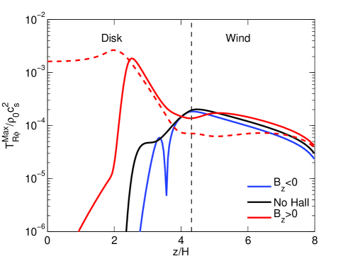
The wind solutions presented in this paper extend earlier wind solutions of Bai & Stone (2013b) and Bai (2013) by including the Hall term, and they share many common properties. The wind launching process is described in Figure 6 and Section 4.1 of Bai & Stone (2013b). For the laminar wind solution, we can divide the disk vertical extent into a disk zone containing the disk midplane where the azimuthal gas velocity is sub-Keplerian, and a wind zone at the disk surface where the azimuthal velocity is super-Keplerian. The height at which this transition occurs, , is referred to as the base of the wind (Wardle & Koenigl, 1993).
The wind carries away disk angular momentum, the rate of which is determined by the component of the stress tensor at the base of the wind (Bai & Stone, 2013b)
| (12) |
Note that only the Maxwell (magnetic) component is involved, because the Reynolds (hydrodynamic) component is simply zero at by definition. The value of is typically found to be or higher in the inner disk.
The total rate of angular momentum loss from the disk is given by the difference of the above stress at the top and bottom of the disk, . Since is constant throughout the disk, the desired symmetry for the wind to extract disk angular momentum is the even- symmetry, where
| (13) |
hence the radial field bends to the same direction at the top and bottom of the disk. Correspondingly, the rate of wind-driven accretion is given by
| (14) |
where subscript ’V’ represents accretion driven by vertical angular momentum transport, and in the latter estimate, we have adopted the MMSN disk model, with being disk radius normalized to AU.
In numerical simulations containing both sides of the disk, it was found that the simulations sometimes generate solutions with odd- symmetry (, ), which is unphysical for a disk wind since it implies that the radial field at the top and bottom bending to opposite directions. This may be due to limitations of the shearing-box framework, where disk curvature is ignored, and hence there is no distinction between inward or outward radial directions. Detailed discussions can be found in Section 4.4 of Bai & Stone (2013b), where it was found that with Ohmic resistivity and AD included, a physical solution can be obtained and maintained by flipping the horizontal field at one side of the disk. However, the physical solution does not strictly obey the even- symmetry: the flip does not exactly take place at the disk midplane, but at some height above through a thin layer. This is because the midplane region is too resistive to conduct electric current, and only in the upper layer (typically at ) can the flip take place where there is marginal coupling between gas and magnetic field. The thin layer carries a strong current, and receives the entire Maxwell stress from the wind. Correspondingly, it possesses large radial velocities and carries the entire accretion flow.
Despite this issue with the symmetry of the wind solution, it was found that the solution in the wind zone, in particular, , is independent of such symmetry (see Section 4.4.1 of Bai & Stone, 2013b for details). This is mainly because is typically higher than the location where horizontal field flips. For this reason, if we are mainly interested in the properties of the disk wind, it suffices to enforce the even- symmetry by simulating half the disk () with reflection boundary condition.
2.6. Radial Transport of Angular Momentum
Besides vertical extraction of angular momentum via disk wind, angular momentum can be transported radially outward within the disk, characterized by the component of the stress tensor
| (15) |
where the overline represents horizontal average. The Shakura-Sunyaev is obtained by vertically integrating across the disk zone
| (16) |
Assuming steady state accretion, the accretion rate resulting from radial angular momentum transport then reads
| (17) |
where subscript ‘R’ represents accretion driven by radial angular momentum transport, and in the second equation we have adopted the MMSN disk model.
In the case of MRI turbulence, and are typically dominated by contributions from turbulence, while in MRI inactive regions, substantial Maxwell stress can be achieved due to large-scale magnetic field (Turner & Sano, 2008). Such large-scale field corresponds to ordered horizontal magnetic field that winds up into spirals and transports angular momentum outward by means of magnetic braking. Since we consider pure laminar wind solutions, radial transport of angular momentum is almost completely due to magnetic braking (Bai & Stone, 2013b, and Reynolds stress is typically negligible).
3. Simulation Setup and Parameters
3.1. Method
We use ATHENA, a higher-order Godunov MHD code with constrained transport technique to enforce the divergence-free constraint on the magnetic field (Gardiner & Stone, 2005, 2008; Stone et al., 2008) for all calculations presented in this paper. Non-ideal MHD terms including Ohmic resistivity (Davis et al., 2010), and AD (Bai & Stone, 2011) have been developed for Athena. In this work, we have further implemented the Hall term, with detailed algorithms described in Appendix A, and code tests shown in Appendix B. Following the formulation in Section 2.2, all our simulations are carried out using the shearing-box module with orbital advection (Stone & Gardiner, 2010). We use the HLLD Riemann solver (Miyoshi & Kusano, 2005) with third order reconstruction. Outflow vertical boundary condition is used, where gas density is extrapolated assuming hydrostatic equilibrium, zero-gradient is assumed for velocity and magnetic field except that in the ghost zones is set to zero if the flow is ingoing at the boundary. We also replenish disk mass to compensate for mass loss, although the mass loss is negligible over the duration of most simulations. We always adopt natural unit in the simulations with .
All our simulations are quasi-1D along the disk vertical dimension to construct laminar wind solutions. They are quasi-1D because we use a three-dimensional (3D) simulation box with only cells in the horizontal dimensions. The additional horizontal dimensions were found to be necessary for our time-dependent simulation to properly relax to the laminar wind configuration (Bai & Stone, 2013b). For most of our runs, the vertical domain covers half of the disk, extending from to . Reflection boundary condition at is enforced to achieve the desired even- symmetry for physical wind solutions. We also perform a few simulations with full disk from to to address issues with symmetry and the strong current layer. In the vertical dimension, we use a resolution of 24 cells per , which we find to be sufficient to properly resolve the wind structure (reducing this resolution by a factor of 2 yields essentially the same wind solution).
The magnetic diffusivities , and are obtained self-consistently in the simulations based on a pre-computed look-up table assuming equilibrium chemistry. For and , they are given in and which are independent of for the regimes we consider in this paper (in the absence of abundant small grains). Since we adopt the MMSN disk model with isothermal equation of state, the diffusivity table is two-dimensional providing the diffusivities as a function of density and ionization rate at fixed temperature. The ionization rate includes contributions from stellar X-ray, cosmic rays and radioactive decay, are expressed a function of column density to the disk surface (see Section 3.2 of Bai, 2011a), where fiducially we adopt X-ray luminosity of erg s-1 and X-ray temperature of 5 keV333The X-ray ionization rate calculations have been updated recently by Ercolano & Glassgold (2013) who found results consistent with previous calculations of Igea & Glassgold (1999) which we adopt.. The procedure closely follows the description in Bai & Stone (2013b), with some changes and updates described below.
We have updated our chemical reaction network with the most recent version of the UMIST database (McElroy et al., 2013). Reactions are extracted using the same list of chemical species adopted in our previous works (Bai & Goodman, 2009; Bai, 2011a, b; Bai & Stone, 2013b; Bai, 2013), which originated from the work of Ilgner & Nelson (2006). The total number of gas-phase reactions increases from 2083 to 2147. The grain-binding energy of all species are also updated to new values. We have tested the new chemical network and found that for a grain-free calculation, the new network gives ionization fractions that are typically slightly smaller compared with the previous version, but within a factor of . Fiducially, we include a single population of dust grains with size m and abundance of in mass, which is the same as used in our earlier works (Bai & Stone, 2013b; Bai, 2013). While this is by no means realistic, it provides reasonable and representative amount of total surface area to enhance recombination. It has been shown that the properties of wind solutions depend very weakly on the grain abundance (Bai & Stone, 2013b), mainly because the wind is launched from disk upper layers where ionization fraction grain abundance.
The disk surface layer is also exposed to far-UV (FUV) radiation which greatly enhances the level of ionization (but is not captured in our diffusivity table) so that the gas behaves in the ideal MHD regime. In our previous works (Bai & Stone, 2013a; Bai, 2013), we obtained the diffusivities in the FUV layer separately by assuming constant ionization fraction of , and the FUV layer was assumed to have a penetration depth of g cm-2 based on the work by Perez-Becker & Chiang (2011a). Correspondingly, there is a sharp jump of diffusivities across the FUV ionization front (see the lower left panel of Figure 5 in Bai & Stone, 2013b). More self-consistent X-ray and UV radiative-transfer calculations (e.g., Walsh et al., 2010, 2012) showed that the ionization fraction increases smoothly from midplane to surface. To avoid unrealistically sharp transitions, we empirically treat the FUV ionization as another independent ionization source, with ionization rate of
| (18) |
The ionization is assumed to act on hydrogen and helium in the same way as X-ray and cosmic-rays so that we can simply use the diffusivity table by extending it to higher ionization rates. This assumption is by no means physical (FUV ionization does not act on H or He), but it works for our purpose, because we simply need a prescription to allow the gas to behave in the ideal MHD regime in the FUV layer with a smooth transition. The detailed ionization structure in the FUV layer is unimportant. To further validate this choice, we have calculated the ionization profiles at 1, 10 and 100 AU based on the above ionization rate at the disk surface, and compared the results with the radiative transfer and chemistry calculations of Walsh et al. (2012) with the same X-ray luminosity and temperature444We sincerely acknowledge H. Nomura and C. Walsh for rerunning their calculations with new parameters and providing us the data for comparison.. We find reasonable agreement when g cm-2, which will be the standard value we adopt in this paper.
From our chemistry calculations, the magnetic diffusivities at the disk midplane can become excessively large, leading to extremely small timesteps from the Courant condition. Besides using super time-stepping to handle Ohmic resistivity and AD (see Appendix A), we further set a diffusivity floor so that . If the floor value is reached, the values of , and are reduced proportionally so as not to affect their relative importance. We have verified that this floor value is sufficiently large and the properties of our wind solutions are independent of 555Increasing the floor value by a factor of 3 has no influence to our fiducial run R1b5H+, while for our run with full box R1b5H+Full, the value of is increased by ..
3.2. Simulation Runs
Our simulations mainly have two parameters, namely, the radial location in the disk , and the net vertical magnetic field characterized by . For each combination of the two parameters, we have three simulation runs. We begin by including only the Ohmic resistivity and AD, running to where the system has fully settled into a laminar configuration. We then turn on the Hall term and split the simulation into two more runs: one is continued from the first run, with (aligned), and for the other we flip all three components of the magnetic field (anti-aligned), while keeping the velocities unchanged. These simulations are run for another orbits to , which is sufficient for the system to relax to a new wind solution.
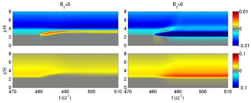
Our simulation runs are named as run RbH, where represents disk radius in AU, , and can be , ‘’, ‘’ denoting initial simulation without the Hall term (), continued simulation with Hall term for (‘’) and (‘’), respectively. For instance, in Section 4, we focus on our fiducial runs R1b5H, which are fixed at AU with . We show in Figure 1 the time evolution of horizontal magnetic field profiles around the time the Hall effect is turned on. The steady state profile prior to belongs to run R1b5H0, after which the two runs evolve differently due to different field polarities. In Section 4.2, we also perform simulations with full vertical domain to address the symmetry issues, named as R1b5HFull. These runs and results and listed in Table 1.
In Section 5, we first consider the fiducial runs with variations in other parameters, also listed in Table 1. The variations are labeled by attaching additional letters in front of the standard run names. We consider disk masses that are and times the MMSN disk, labeled by ‘M3’ and ‘M03’. We also perform runs with grain-free chemistry, labeled by ‘nogr’. Finally, we vary the X-ray ionization rate to and ergs s-1, labeled by ‘X29’ and ‘X31’. In the remainings of Section 5, we further consider runs with and , and at 0.3, 3, 5, 8 and 15 AU, where all other parameters are fixed at standard values. The list of these simulation runs are provided in Table 2.
4. Simulation Results: Representative Wind Solutions
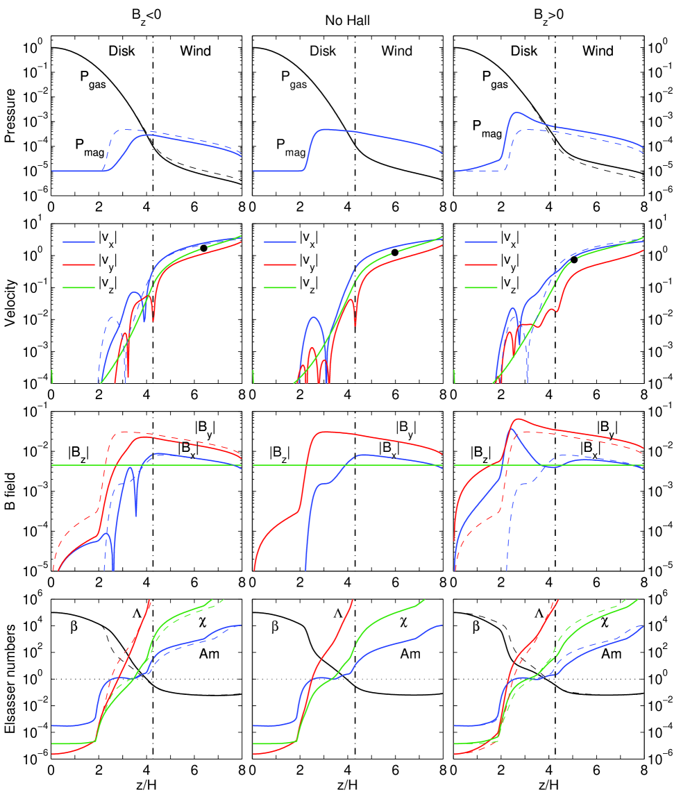
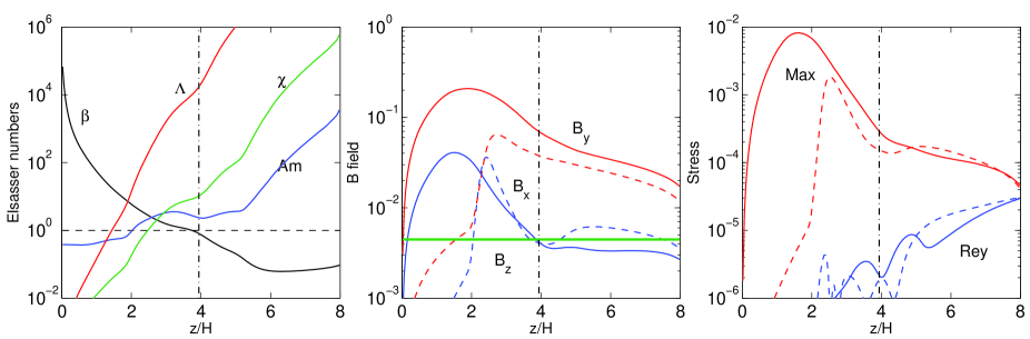
We begin by focusing on a fiducial set of simulations at fixed radius of 1 AU with . In Figure 2, from left to right, we show the general properties of the wind solutions for runs R1b5H–, R1b5H0 and R1b5H+ respectively. Major diagnostic quantities of these solutions are provided in Table 1. The rest of this section is devoted to discussing the properties of these solutions.
4.1. Relaxation to New Wind Solutions
We start from the middle panels of Figure 2 for run R1b5H0, where the Hall term was not included. The solution closely resembles the fiducial solution in our previous work Bai & Stone (2013b) (see their Figures 5, 11 for solutions with odd and even symmetries), except that the Elsasser numbers in this work increase smoothly to the surface FUV layer as a result of the new procedure adopted in this work. While the depth of the FUV layer is uncertain, such smooth transition is likely more realistic.
Solutions including the Hall effect (R1b5H) are shown in the left and right panels of Figure 2. We see that the main effect is that the horizontal magnetic field is strongly amplified when , while the field is largely reduced when . The amplification and reduction mainly result from the Hall-dominated region at . Moreover, for , the sign of reverses in the Hall-dominated region so that it has the same sign as . In our time-dependent simulations, relaxation from the original solution R1b5H0 to the new solutions R1b5H is very rapid, as we see in Figure 1. The initial evolution of takes less than an orbit, with a few more orbits to fully relax to the final configuration.
These features can be understood by looking at the induction equation. With the addition of the Hall term, the immediate evolution of magnetic field follows
| (19) |
| (20) |
where is the Hall diffusivity based on vertical magnetic field, assumed to be constant to facilitate the analysis, and represents changes in to account for additional shear conversion of to .
The first equation (19) describes the generation of radial field due to the Hall effect. The underlying physics is best understood from the grain-free expression of in Equation (7): Vertical gradient of toroidal field provides radial current , corresponding to radial drift of electrons relative to the ions. In the Hall dominated regime, the ions are coupled to the neutrals , while magnetic field is frozen to the electrons. The second -derivative then descries conversion of vertical field into radial fields due to vertical shear of electron motion. Depending on the sign of (hence ), the result is that the original radial field can be amplified () or reduced () once the Hall term is turned on, as we see in Figure 2.
The second equation (20) provides positive feedback to field evolution due to shear. For , shear conversion from amplifies the toroidal field (and in general its second derivative), which promotes additional amplification of the radial field via (19), leading to runaway. This is closely related to the Hall-shear instability of Kunz (2008), as also pointed out in Lesur et al. (2014). We see from Figure 2 that the radial field is substantially stronger than the Hall-free case throughout the disk interior. Similarly, the toroidal field also becomes much stronger than the Hall-free case. The field amplification process is eventually saturated due to damping by Ohmic resistivity and AD, as well as advection of magnetic field by disk outflow.
The opposite applies when . The Hall effect and shear act destructively to the Hall-free field configuration and both radial and toroidal magnetic fields are reduced. In particular, we see from the left panels of Figure 2 that the radial field even changes sign around due to the Hall effect, hence and have the same sign (but small amplitude) around this region, giving a negative Maxwell stress. While shear conversion tends to reverse the sign of as well, this does not occur due to AD.
4.2. Issues with Symmetry
While we have enforced reflection symmetry across the disk midplane to guarantee that the wind solutions have physical geometry, it remains to clarify to what extent this assumption can be justified. In particular, in the case of , this treatment forces and to zero at the midplane, which works against magnetic field amplification. To this end, we perform a set of additional simulations containing the full disk with fiducial parameters (1AU, with two polarities), named R1b5HFull.
In these simulations, we follow a similar procedure by starting with a Hall-free run to , and then turn on the Hall effect for the two polarities. The Hall-free run saturates into the odd- symmetry solution (unphysical for the wind), where the horizontal magnetic field maximizes at the midplane. After turning on the Hall effect, the same symmetry remains, which we run to time for full relaxation. At this time, we manually flip the horizontal magnetic field and velocity field at all cells with to achieve the physical even- symmetry. We then continue to run the simulations to and focus on how the system relaxes. We call these two continued runs R1b5HFull. For comparison, we also apply the flip to the Hall-free simulation, which is named as R1b5H0Full.
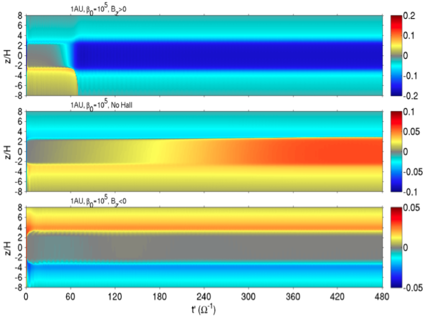
In Figure 3, we show the time evolution of the toroidal field profiles from these the runs after the flip (we set at the time of flip). In the Hall-free case, we see that the system maintains the even- symmetry state for a few orbits, while asymmetry slowly develops and the midplane toroidal field is gradually amplified with a single sign. Nevertheless, the magnetic field configuration in the wind zone (surface layer) remains unchanged, and the system eventually relaxes to the physical wind solution with a strong current layer offset from disk midplane at , as highlighted in Bai & Stone (2013b).
4.2.1 The Case
With the Hall effect, and when , we see that the initial evolution of the system is similar to the Hall-free case, but in 10 orbits, the midplane field gets rapidly amplified (as a result of the Hall-shear instability), and the horizontal field flips back to arrive at the odd- symmetry solution. There is a transient phase (around ) where the field configuration remains physical for a disk wind and contains a strong current layer at , but the field amplification is so rapid that a unidirectional toroidal field quickly overwhelms and spreads into the entire disk. Overall, it appears that with strong field amplification due to the Hall-shear instability, the even- symmetry solution is difficult to be maintained in shearing-box without manually enforcing the symmetry at the midplane666However, this can be achieved at outer disk radii, as we will demonstrate in the forthcoming paper with an example at 5 AU.. In addition, achieving a physical wind solution with a strong current layer offset from the midplane appears difficult as well. This point was also raised in Lesur et al. (2014) based on their simulations.
The above fact poses serious concerns about the physical reality of the system at AU: one either achieves the odd- symmetry solution with unphysical wind geometry, or achieves the more physical even- symmetry solution by unrealistically restricting the field geometry. This apparent dilemma may reflect the limitations of the shearing-box framework, and global simulations will be the key to resolving these issues. While we choose to restrict the symmetry in our simulations for most of this work, readers should bare in mind the potential caveats.
4.2.2 The Case
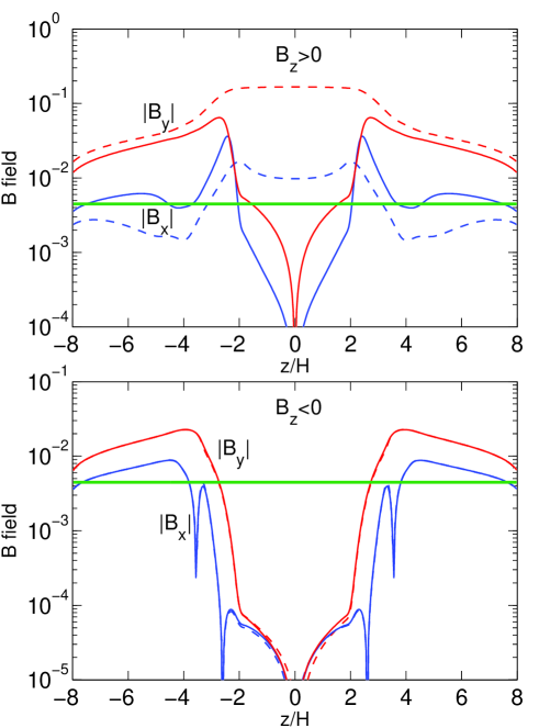
When , on the other hand, we see from the bottom panel of Figure 3 that the physical even- symmetry solution we obtained earlier easily survives in the full-disk simulation. The bottom panel of Figure 4 further compares the full-disk solution with our previous solution with enforced reflection symmetry. The agreement is almost exact. Therefore, we conclude that for the case, a wind solution with physical geometry exists naturally, where the horizontal field diminishes around the midplane region due to the Hall effect and transitions through zero.
4.3. General Properties of the New Wind Solutions
As introduced in Section 2.5, we separate the wind solution into a disk zone and a wind zone. They are divided at , the base of the wind. Conventionally, is defined as the point where the azimuthal velocity transitions from sub-Keplerian to super-Keplerian (Wardle & Koenigl, 1993), which is adopted in our previous studies (i.e., in shearing-box simulations). For our new wind solutions, we find that this location is well defined when , as can be seen from the second row of Figure 2, where shows a clear kink in the logarithmic plot at about . This is only slightly smaller than in the Hall-free run R1b5H0. When , we see that at about the same location, undergoes a minimum but does not reverse sign. Since other aspects of this solution does not change significantly, we modify the definition of as follows: moving from disk surface downward, is located at where experiences a minimum for the first time. This definition maintains consistency with our Hall-free run R1b5H0. Also, for run R1b5H+, the Reynolds stress is minimized at and is negligible compared with the Maxwell stress .
Below we discuss the general properties of the new wind solutions, focusing on the fiducial (half-disk) runs R1b5H. For the case, we further compare the wind properties between half and full-disk simulations at the end of this subsection.
4.3.1 Angular Momentum Transport by Disk Wind
Angular momentum transport by disk wind has been discussed in Section 2.5. With the physical wind symmetry as enforced in our simulations, the wind-driven accretion rate is proportional to the wind stress , and can be estimated by Equation (14). Their values are provided in Table 1. For our fiducial runs R1b5H, the wind-driven accretion rates in both magnetic polarities are well above the desired value of yr-1.
We see that including the Hall term, the wind-driven accretion rates are modestly increased (reduced) in the case of () compared with the Hall-free run R1b5H0. Since with being constant in the disk, the modest increase/reduction is directly related to the amplification/reduction of discussed in Section 4.1.
4.3.2 Radial Transport of Angular Momentum
Radial transport of angular momentum via magnetic braking has been discussed in Section 2.6. In Figure 5 we show the vertical profiles of from our fiducial runs. In Table 1 we further list the value of , and the corresponding assuming an MMSN disk. We see that including the Hall term, is substantially enhanced (reduced) in the case of (). For , the enhancement of is greatest in the Hall-dominated region (). This mainly results from magnetic field amplification as discussed in Section 4.1. We see from Figure 2 that in this region is amplified by more than an order of magnitude compared with the Hall-free case. Together with modestly amplified , they both contribute to enhance the total by a factor of compared with the Hall-free case. For , the reduction and reversal of together with reduced naturally leads to much smaller .
The radial transport of angular momentum via magnetic braking was mentioned but not emphasized in our earlier work of Bai & Stone (2013b), since its contribution is much smaller than that from wind-driven accretion. With the Hall effect and aligned magnetic field, however, magnetic braking already contributes a non-negligible fraction of the angular momentum transport, as read from Table 1, and this term alone is sufficient to account for the typically observed accretion rates in PPDs. On the other hand, for anti-aligned magnetic field geometry, contribution from magnetic braking is completely negligible.
| Run | ||||||||||
| R1b5H+ | 0.89 | |||||||||
| R1b5H0 | 0.10 | |||||||||
| R1b5H– | ||||||||||
| R1b5H+Full | 3.67 | – | – | |||||||
| R1b5H0Full | 0.18 | |||||||||
| R1b5H–Full | ||||||||||
| M03-R1b5H+ | ||||||||||
| M03-R1b5H0 | ||||||||||
| M03-R1b5H– | ||||||||||
| M3-R1b5H+ | ||||||||||
| M3-R1b5H0 | ||||||||||
| M3-R1b5H– | ||||||||||
| nogr-R1b5H+ | ||||||||||
| nogr-R1b5H+Full | ||||||||||
| nogr-R1b5H0 | ||||||||||
| nogr-R1b5H– | ||||||||||
| X29-R1b5H+ | 0.40 | |||||||||
| X29-R1b5H0 | 0.11 | |||||||||
| X31-R1b5H+ | 1.51 | |||||||||
| X31-R1b5H0 | 0.15 | |||||||||
| X31-R1b5H–∗ | 0.059 |
See Section 3.2 for description of simulation runs and naming conventions. The last run (with ∗) is eventually unstable, where values are taken before the instability takes over. The results are mainly discussed in Section 5.1.
List of physical quantities in the Table are, : Shakura-Sunyaev due to Maxwell stress (magnetic braking); : accretion rate due to radial transport of angular momentum ( yr-1); : the wind stress (natural unit); : wind-driven accretion rate ( yr-1); : single-sided mass outflow rate (), : maximum inflow velocity (); : location at the maximum inflow velocity (), : radial drift velocity of vertical magnetic flux; : location of the base of the wind; : location of the Alfvén point.
| Run | ||||||||||
| R03b5H+ | ||||||||||
| R03b5H0 | ||||||||||
| R03b5H- | ||||||||||
| R03b6H+ | ||||||||||
| R03b6H0 | ||||||||||
| R1b4H+ | ||||||||||
| R1b4H0 | ||||||||||
| R1b4H– | ||||||||||
| R1b5H+ | 0.89 | |||||||||
| R1b5H0 | 0.10 | |||||||||
| R1b5H– | ||||||||||
| R1b6H+ | ||||||||||
| R1b6H0 | ||||||||||
| R3b4H+ | ||||||||||
| R3b4H0 | ||||||||||
| R3b4H– | ||||||||||
| R3b5H+ | ||||||||||
| R3b5H0 | ||||||||||
| R3b6H+ | ||||||||||
| R5b4H+ | ||||||||||
| R5b4H0 | ||||||||||
| R5b4H– | ||||||||||
| R5b5H+ | ||||||||||
| R5b5H0 | ||||||||||
| R5b6H+ | ||||||||||
| R8b4H+ | ||||||||||
| R8b4H0 | ||||||||||
| R8b5H+ | ||||||||||
| R8b6H+ | ||||||||||
| R15b4H+ |
Same as Table 1, and see Section 3.2 for description of simulation runs and naming conventions. Results are mainly discussed in Section 5.3-5.4.
4.3.3 Wind-driven Accretion Flow
In our simulations, the wind stress directly leads to an inward accretion mass flux, while there is no mass flux associated with radial angular momentum transport due to the shearing-sheet formulation where radial gradients are ignored. Here we focus on the wind-driven accretion mass flux.
We see from the second row of Figure 2 that in all three runs R1b5H, the radial velocity transitions from being positive in the wind zone, to negative somewhere below the base of the wind, which corresponds to the accretion flow. Interestingly, the vertical distribution of the accretion flow is different in the three runs: for , the inflow region is located at larger vertical hight compared with the Hall-free case, while for , the inflow is located further toward disk interior. To characterize the basic properties of such inward mass flux, we identify the maximum inflow velocity and the location where it is achieved , and list their values in Table 1.
We note that the location of the inflow corresponds to where the wind stress is exerted to the disk. The vertical gradient of (or effectively ) is directly related to the torque per unit length received by the gas hence the rate of the gas inflow. When , the horizontal magnetic field is amplified toward disk interior, therefore, the inflow region is located closer to the disk midplane. This can be effectively interpreted as that allows the magnetic field to be coupled with the gas deeper toward the midplane. The opposite applies for the case.
4.3.4 Disk Outflow
The outflow mass loss rate in the disk wind is not well characterized in shearing-box simulations. It decreases with increasing the vertical box size, as studied and discussed extensively in Fromang et al. (2013) for the MRI turbulence case and Bai & Stone (2013b) for the laminar wind case. Here, we are not concerned with the absolute mass loss rate, but focus on the relative dependence of the mass outflow rate on physical parameters such as magnetic polarity (this subsection), , and disk radius (Section 5), where shearing-box may provide more reliable results.
The measured mass loss rates from our simulations are listed in Table 1.777Note that the values reported correspond to single-sided mass loss rate, while the Tables in Bai & Stone (2013b) and Bai (2013) quote the mass loss rates from both sides of the disk. We see that when (), the wind mass loss rate is higher (lower) compared with the Hall-free case, consistent with the wind being stronger (weaker) discussed earlier. The increase (reduction) in the outflow mass flux is mainly due to the higher (lower) gas density at , as a result of stronger (weaker) magnetic pressure support. The change in the mass outflow rate is accompanied by the change in the location of the Alfvén point, . It is defined as the location where vertical velocity equals to the vertical Alfvén velocity . As discussed in Bai & Stone (2013b), larger outflow rate makes the Alfvénic point lower, and vice versa (see their Section 4.5).
4.3.5 Magnetic Flux Transport
Poloidal magnetic flux can drift radially in the disk at velocity in the presence of toroidal electric field
| (21) |
where is given in Equation (6). The steady state condition further requires to be constant with height so that magnetic flux drifts uniformly across the disk, giving a single value of . Positive or negative would lead to expulsion or accumulation of magnetic flux.
In Table 1, we show the value of measured from our simulations. We see that without the Hall term, the value of is very close to zero in run R1b5H0, as found earlier in Bai & Stone (2013b). Including the Hall term, deviates substantially from , and is negative (positive) when (). This means that poloidal magnetic flux is transported inward (outward) at large velocities (), much faster than the velocity of the accretion flow.
In reality, the value of should be determined by global conditions and can not be controlled in our local simulations. Therefore, we may expect that the realistic value of should be much closer to zero than what we obtain here. The general properties of the wind solution have been found to depend weakly on the exact value of (Wardle & Koenigl, 1993). Moreover, the measured values of are still much less than the sound speed, hence we do not expect the properties of the supersonic wind to be strongly affected. Overall, the values of listed in Table 1 should mainly be taken for reference but not to be taken seriously for studying magnetic flux transport.
4.3.6 Comparison with Full-disk Simulations
Finally, we compare our fiducial half-disk simulations R1b5H with enforced reflection symmetry with full-disk simulations R1b5HFull. As discussed in Section 4.2, for , the full-disk simulation yields almost exactly the same wind solution as half-disk simulations. Table 1 further confirms that major diagnostics between runs R1b5H and R1b5HFull are almost identical. In the Hall-free case, the wind diagnostics between runs R1b5H0 and R1b5H0Full are also very close, with the full-disk run producing higher , consistent with the results in Bai & Stone (2013b).
Below we focus on the comparison for the case. The top panel of Figure 4 compares the magnetic field profiles between the odd- and even- symmetry solutions. With a full disk, we see that the horizontal magnetic fields and get amplified and maintain its strength across the midplane, instead of being forced to damp to zero within in the half-disk run. As a result, large extends to the midplane, leading to stronger magnetic braking. Reading from Table 1, we see that in run R1b5H+Full is about 4 times higher than in run R1b5H+.
We also notice that at the disk surface, the odd- and even- symmetry solutions do not overlap. This is different from the Hall-free case, where they match each other at the disk surface (Bai & Stone, 2013b). The reason is that odd- symmetry solution (in the full-disk run) requires by construction, thus ; while we have seen the even- symmetry solutions from the half-disk runs have non-zero . Therefore, the odd- symmetry solutions we have obtained are not even- symmetry solutions with flipped horizontal field. Major wind diagnostics listed in Table 1 show that both and are larger in full-disk simulations by about and respectively.
5. Simulation Results: Parameter Study of the Wind Solutions
In this section, we consider much wider range of parameters and discuss how they affect the properties of the new disk wind solutions. We first consider variations to our fiducial solution at 1AU with in Section 5.1, with the list of runs and results shown in Table 1. We then vary the radial location and vertical field strength and discuss the results in Sections 5.2 to 5.4, with the list of runs provided in Table 2. Note that when varying , the ionization profile changes which changes the absolute strength of all non-ideal MHD terms simultaneously, meanwhile, changes in gas density alters the relative importance among the three non-ideal MHD effects, as can be inferred from Equation (7). Correspondingly, Ohmic resistivity becomes progressively less important toward large radii, where AD becomes progressively more prevailing.
5.1. Variations to Fiducial Runs
5.1.1 Disk Surface Density
We first vary the disk surface density by a factor of and (labeled by “M3” and “M03”). Accordingly, we have also varied the strength of the net vertical magnetic field so that the physical value of the field strength remains the same (hence and respectively). Looking from Table 1 we see that the wind-driven accretion rate almost remain identical as in the fiducial run under these variations, for both and . Similarly, the measured wind mass loss rate also remain approximately unchanged when converting from numerical to physical units ( for M03 runs and for M3 runs). The results are consistent with the Hall-free case studied in Bai & Stone (2013b), indicating that the strength of the wind is solely determined by the physical strength of the magnetic field. Also from Table 1, accretion rate driven by magnetic braking is more or less unaffected by the variation of disk surface density.
5.1.2 Grain Abundance
We next consider a run using grain-free chemistry labeled by “nogr”. We find that the strength of the disk wind, characterized by and , is stronger than the fiducial case for both and cases, although the enhancement is only modest, which is again consistent with findings in Bai & Stone (2013b) for the Hall-free case. However, in the case of , the enhancement of (magnetic braking) is substantial. In Figure 6, we show the corresponding Elsasser number, magnetic field and stress profiles for run nogr-R1b5H+. We see that the midplane value of increases by orders of magnitude compared with the fiducial run R1bb5H+, reflecting the increase in midplane ionization fraction. The reduced magnetic diffusivity toward the disk midplane makes magnetic field amplification discussed in Section 4.1 extend to much deeper regions than the fiducial case. We see that it was not until very close to the midplane that the horizontal field starts to drop to zero by enforced symmetry. The deeper penetration with continued amplification that acts to both and , which leads to much stronger Maxwell stress, giving about 10 times larger than the fiducial case.
We can compare our grain-free simulation results with the results of Lesur et al. (2014). They conducted full-disk simulations with an analytical prescription of grain-free chemistry. They obtained , compared with in our case. For fair comparison, we further performed a grain-free run with full disk, obtaining . This is very close to our half-disk simulation result magnetic field amplification proceeds to the midplane in both cases. This value is a factor of smaller than their result mainly because our grain-free chemistry calculation is based on a complex chemical reaction network that yields smaller ionization fraction than their analytical formula (checking the midplane value indicates a factor of difference). Lesur et al. (2014) also reported that the midplane magnetic field is amplified to equipartition level and strongly affects the disk hydrostatic equilibrium. In our full-disk grain-free simulation, we find the total at disk midplane and drops below at (to affect hydrostatic structure). This is again because of the lower ionization fraction from our grain-free chemistry.
5.1.3 Ionization rate
Finally, we vary the X-ray luminosity to and ergs s-1 to study the role of X-ray ionization on wind properties. The range of variation reflects the observed scatters of X-ray luminosities in young stars (Preibisch et al., 2005), and may also account for the fact that X-ray luminosities in young stars are highly variable (Wolk et al., 2005). We find that reducing the X-ray luminosity only modifies the properties of the wind slightly, which is mainly because the wind is launched from the surface layer dominated by FUV ionization. On the other hand, increasing the X-ray luminosity leads to modest increase of the wind strength by allowing the wind to be launched from deeper regions (due to enhanced ionization, see the values of in Table 1).
Most interestingly, we find that the wind solution becomes unstable in the case with enhanced X-ray ionization888For with , we find similar unstable behavior for more subtle reasons.. In Figure 7 we show the time evolution of the horizontal magnetic field in our run X31-R1b5H. After turning on the Hall term at , system quickly relaxes to a new configuration, but then becomes unstable and the horizontal field flips in less than 10 orbits. This flip phenomenon repeats itself quasi-periodically. The cause of the flip, as well as the consequences, will be discussed in the next subsection in combination with a wider range of runs. Despite being unstable, the bulk of the configuration still consists of a disk wind. The values shown in Table 1 for this run are obtained by measuring the wind properties from , and we see from all major diagnostics that the strength of the wind is also modestly enhanced compared with the Hall-free case.

5.2. Parameter Space of Stable Wind Solutions
We then perform a series of quasi-1D simulations with different and at different disk radii. We find some of the quasi-1D runs never relax to a steady state. Instead, they show similar behaviors as our run X31-R0b5 with the large-scale horizontal field changing sign quasi-periodically. Whenever this happens, steady state wind solution is unlikely possible, and we do not include these runs in Table 2.
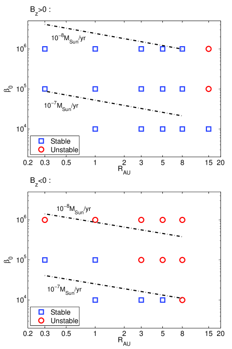
In Figure 8 we show the stability map for all the quasi-1D simulations we performed in the parameter exploration of and . Compared with the Hall-free situation of Bai (2013) (see his Figure 7), it is clear that when , the parameter space for stable wind solutions is considerably enlarged: stable solutions can be found with weaker vertical field and outer disk radii; while if , the parameter space for stability is largely reduced: stable solutions can only be found with stronger vertical field and at smaller disk radii.
The onset of the instability in the unstable runs is due to the MRI, and the observed stability trend can be readily understood from the Hall-MRI linear dispersion relation.
As discussed in Section 2.4, the main reason for the existence of stable (Hall-free) wind solutions is that the MRI unstable modes under the given vertical field strength become too long to fit into the disk. The main role played by the Hall effect is that, for , the unstable MRI modes shift to smaller , or longer wavelength at fixed vertical field (Wardle, 1999, and see Figure 12 in the Appendix). Therefore, to make the system unstable, further weaker vertical field (smaller ) is required. This explains why the parameter space for stability is enlarged when .
For (or ), unstable MRI modes exist only when . Without dissipation, the unstable modes essentially extends to infinitely small scales for (Wardle, 1999). With dissipation, mostly ambipolar diffusion, the unstable modes cutoff at finite wavelength, yet still extend to scales smaller than the Hall-free case. This can again be seen from Figure 12 in the Appendix999Since the MRI dispersion relation in the presence of pure vertical field is identical for the case with Ohmic resistivity and AD (Wardle, 1999), one can simply replace by in that figure to see the trend.. Since transitions from to from midplane to surface, it always falls in this range at certain height. At this location, the unstable MRI modes extend to shorter wavelength for fixed vertical field, making it more susceptible to the MRI. Indeed, when checking with Figure 7 as well as many other unstable runs, we find that regions that first lead to instability (at in Figure 7) are typically associated with transition through order unity.
The above discussions are also consistent with the analysis of the MRI linear modes presented by Wardle & Salmeron (2012).
Connecting to the discussions at the end of the previous subsection (5.1), we note that the range of stability can depend on other parameters such as grain abundance and X-ray ionization. It is conceivable that, for example, with enhanced X-ray ionization and reduced grain abundance, the range of radii where the laminar wind solution holds would shrink, at least in the case of .
5.3. Solutions toward Outer Radii
Toward outer disk radii, external ionization penetrates deeper into the disk midplane. Together with reduced gas density, this leads to rapid increase of the ionization fraction, making the disk midplane region better coupled to magnetic field. Two consequences result. First, the wind is launched from a lower height compared with our fiducial runs, leading to higher mass outflow rate and wind stress (in code units). This has been discussed in Bai (2013). Second, with the Hall effect, this makes magnetic field amplification more prominent in the case.
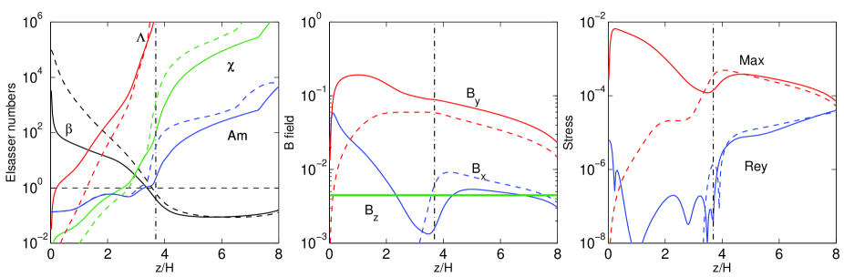
In Figure 9, we show the profiles of the Elsasser numbers, the three magnetic field components, and the stresses from our runs R5b5H0 and R5b5H+ (note that run R5b5H is MRI unstable). We see that in the Hall-free case, the radial field diminishes well before reaching the midplane. With the Hall term, continues to increase toward the midplane until it catches up with the toroidal field before diminishing to zero at the midplane enforced by symmetry. The strongly enhanced combined with makes the Maxwell stress more than times larger than the Hall-free case. This example is an exaggerated version of the 1AU fiducial runs discussed in detail in Section 4.1. It is similar to the grain-free run discussed in Section 5.1, and also other wind solutions at comparable or larger radii listed in Table 2 are qualitatively similar. We also note that at radius AU, the location of maximum inflow velocity is either very close or exactly at the disk midplane, indicating that entire disk is actively coupled to the magnetic field.

Despite the stronger magnetic coupling in the midplane region, the properties of the wind seem to be less affected, as we see that to the right of the vertical dash-dotted line in Figure 9, the magnetic profile, as well as the Maxwell and Reynolds stresses behave in a way very similar to the 1 AU case.
5.4. Angular Momentum Transport and Mass Outflow
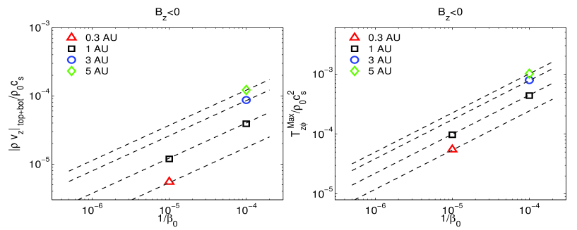
In this subsection, we follow the approach of Bai (2013) and study the dependence of the wind-driven accretion rate on and . Using all the data from Table 2, we fit the wind mass loss rate and the wind stress in the form of , where , and are constants.
For , there are a total of 15 data points, we find
| (22) |
| (23) |
For , although there are only 5 data points, we find a very tight fit
| (24) |
| (25) |
In the above two formulas, uncertainties to all fitting coefficients are found to be less than . The inclusion of surface density in these relations is based on the discussions in Section 5.1.1.
Without the Hall term, the fitting results are very close to Equations (9) and (10) of Bai (2013), thus we do not repeat. Also note that we have quoted single-sided mass loss rate while Bai (2013) used mass loss rate from both sides.
In Figures 10, we show the values of the wind mass loss rate and the wind stress from all runs in Table 2 together with the above formulas. We see that these formulas generally fit the data very well. The power law indices of the scaling relations are similar indicating similar wind physics. We have also checked the scalability of and find that while it has the trend to monotonically increase with increasing magnetic flux, the dependence on is not monotonic.
Interpretation of these fitting formula follows from the discussions in Section 3.2 of Bai (2013). With proper unit conversion, i.e., Equation (14), the wind stress should provide reliable estimates of the wind-driven accretion rate. When applied to disks with surface density , one should interpret as the ratio of the midplane gas pressure of a MMSN disk to the magnetic pressure of the net vertical field. The wind mass loss rate , on the other hand, is not well determined in the shearing-box framework (Fromang et al., 2013; Bai & Stone, 2013b). The normalization factors in the fitting formulas are likely significant overestimated, while power-law indices are probably more reliable, which at least sets the benchmark for shearing-box simulations.
Using these fitting formulas and Equation (14) assuming MMSN disk, we further show in Figure 8 in dash-dotted lines the desired value of as a function of for the disk to maintain wind-driven accretion rate of and yr-1. We see that given the typical accretion rate of yr-1, stable wind solutions for disks with extend up to AU, while for disks with , stable solutions exist only up to 3-5 AU. Reducing the accretion rate would lead to reduced radial range of stability.
Based on the fact that wind-driven accretion rate depends only on the physical strength of the net vertical field , we can further write down the wind-driven accretion rate in terms of the physical field strength
| (26) |
for , and
| (27) |
for . These expressions can be considered as disk-model independent, as long as a stable laminar-wind solution exists. The only MMSN scaling comes from the temperature profile, which is reasonable for irradiated disks.
The above formulas are to be compared with the Hall-free formula based on the results of Bai (2013) 101010We regret the miscalculation in Equation (11) of Bai (2013).
| (28) |
These formulas again capsulate the role of the Hall term on the properties of the laminar wind solutions. With similar scalings, they reveal the enhancement and reduction on the strength of disk wind introduced by the Hall term when or .
Our results indicate that mG net vertical magnetic field is necessary to achieve wind-driven accretion rate of yr-1 at 1 AU. Stronger field is required for the case and weaker field for . For steady-state accretion, the radial profile of should satisfy for both magnetic polarities, corresponding to magnetic flux distribution of , where denotes the total magnetic flux contained within radius .
6. Summary and Discussion
6.1. Summary
In this work, we have successfully implemented the Hall term in the ATHENA MHD code, which enables us to extend our previous study on the gas dynamics of protoplanetary disks (PPDs) to include all three non-ideal MHD effects in a self-consistent manner in local shearing-box simulations. All our simulations include an external vertical magnetic field , which has been realized to be essential (see discussions in Section 2.4). We focus on the inner region of PPDs (up to AU) in this paper where the disk is expected to be largely laminar with accretion driven by a magnetocentrifugal wind.
Our first important finding is that including the Hall term, the conclusion from our previous work (Bai & Stone, 2013b; Bai, 2013 where only Ohmic resistivity and ambipolar diffusion were included) that the inner disk is largely laminar still holds, with accretion mainly driven by a magnetocentrifugal wind. On the other hand, the wind solution is further controlled by the Hall effect in a way that depends on the polarity of the external vertical field (sign of ), and we summarize as follows.
For external field being aligned with disk rotation (), we find
-
•
The horizontal magnetic field is strongly amplified compared with the Hall-free solutions due to the Hall-shear instability, leading to stronger disk wind and more efficient (vertical) angular momentum transport by up to .
-
•
The enhanced horizontal magnetic field drives radial transport of angular momentum via large-scale Maxwell stress (magnetic braking), which accounts for a considerable fraction of the wind-driven accretion rate.
-
•
The parameter space where a stable laminar wind solution can be found is extended. For typical accretion rates of yr-1, radial range of stability extends to AU before the MRI sets in.
For external field being anti-aligned with disk rotation (), we find
-
•
The horizontal magnetic field is reduced compared with the Hall-free solutions, leading to weaker disk wind and less efficient (vertical) angular momentum transport by .
-
•
Radial transport of angular momentum by magnetic braking is negligible.
-
•
The parameter space for a stable laminar wind solution is substantially reduced. For typical accretion rates of yr-1, radial range of stability extends only to AU before the MRI sets in.
For our fiducial simulation parameters (1AU with ), we explored the dependence of the wind solutions on the disk surface density, X-ray ionization rate and grain abundance. Our results indicate that the wind properties are largely determined by the physical strength of the vertical magnetic field. They are independent of the disk surface density and weakly dependent on the ionization structure (e.g., grain abundance, ionization rate). On the other hand, the efficiency of magnetic braking strongly depends on the diffusivity profiles, and grain-free chemistry yields much higher than calculations with grains.
Using the MMSN disk model, and using standard prescriptions of ionization and chemistry, we further explored the dependence of the wind properties on disk radii and the strength of the vertical magnetic field. The results are best summarized in the fitting formulas (22) to (25). We also provide disk model independent formulas for the wind-driven accretion rate in Equations (26) and (27). Our results indicate that mG net vertical magnetic field at 1 AU is required to account for the typical PPD accretion rates. At fixed accretion rate, stronger (by a factor of ) net field is needed in the case.
Most of our simulations cover half of the disk with enforced reflection boundary condition at the disk midplane to guarantee that the wind solutions obey the even- symmetry (horizontal magnetic field changes sign at midplane). We find that in the case, these solutions can always be realized when using a full disk thanks to the Hall effect, which reduces horizontal field strength toward the disk midplane. When , however, we are currently unable to achieve the even- wind solutions in full-disk simulations at AU. The system tends to end up at the odd- symmetry solution where the outflow geometry is unphysical for a disk wind. This solution gives stronger magnetic braking by a factor of up to a few since horizontal magnetic field is amplified throughout the midplane instead of passing through zero. While it is unclear which solution the nature picks due to limitations of the shearing-box framework, we do find that the even- symmetry wind solution can be realized at slightly larger disk radii ( AU), which we will discuss in our companion paper. Finally, the even- wind solutions obtained via simulations tend to have large radial drift velocities of magnetic flux, which is likely affected by vertical boundary conditions. Global simulations are essential to resolve the symmetry issues and to yield realistic rate of magnetic flux transport.
6.2. Discussions
Our work strengthens the notion that the evolution of PPDs is largely governed by the distribution and transport of external poloidal magnetic flux, as suggested in our previous works (Bai & Stone, 2013b; Bai, 2013). Such large-scale field is expected as a natural consequence of star formation: molecular clouds and star-forming cores are all strongly magnetized (e.g., see Crutcher, 2012 for a review). Recent dust polarization observations further reveal the presence of large-scale field threading protostellar cores. The large-scale fields appear to be randomly oriented with respect to the direction of protostellar outflows (Hull et al., 2014), while there is also evidence of preferential alignment for more isolated sources with projection effects taken into account (Chapman et al., 2013). Considering the Hall effect, the bifurcation of disk wind properties with different polarities of the external magnetic field further suggests that PPDs may evolve differently with different initial magnetic field polarities, and systems with may achieve higher accretion rate, or retain less magnetic flux (in a self-organized way to avoid accreting to fast) compared with systems with .
On the other hand, the desired level of magnetic flux threading PPDs (at least in the Class II phase) is tiny compared with the amount of magnetic flux threading star-forming cores. Consequently, the process of star formation must also be accompanied by the removal of magnetic flux, which is another major problem in the theory of star formation. It appears that substantial magnetic flux must be removed in order to form the PPD itself to avoid the “magnetic braking catastrophe” (Mellon & Li, 2008), which may be achieved via misaligned magnetic field (Hennebelle & Ciardi, 2009; Joos et al., 2012), external turbulence (Santos-Lima et al., 2012; Seifried et al., 2012) or non-ideal MHD effects (Li et al., 2011; Krasnopolsky et al., 2011; Tomida et al., 2013). After disk formation, the transport of magnetic flux must be achieved within the disk itself, yet the problem is intrinsically global, and must depend on the overall magnetic field geometry and internal dissipation in the disk (e.g. Lubow et al., 1994). Recently, there have been several semi-analytical works to study magnetic flux transport in thin accretion disks which have revealed complex dependence on the internal disk microphysics (e.g., Guilet & Ogilvie, 2012, 2013; Okuzumi et al., 2013; Takeuchi & Okuzumi, 2013). Nevertheless, a still missing important ingredient is the launching of magnetic outflow, and it appears that global simulations of PPDs with resolved disk microphysics and sufficiently large vertical domain to accommodate disk outflow is essential toward a better understanding.
While our results suggest the inner region of PPDs is largely laminar in terms of magnetic activities, it does not exclude the possibility for pure hydrodynamic mechanisms to generate turbulence. In fact, some level of turbulence is probably needed to keep at least some small dust suspended in the disk so as to explain the scattered starlight as well as the near infrared spectral energy distribution (e.g., Stapelfeldt et al., 2003; D’Alessio et al., 2006). Promising candidates of hydrodynamic turbulence may include the Goldreich-Schubert-Fricke instability (Urpin, 2003; Nelson et al., 2013), the critical layer instability (Marcus et al., 2013) and the convective overstability and baroclinic vortex amplification (Petersen et al., 2007; Lesur & Papaloizou, 2010; Raettig et al., 2013; Klahr & Hubbard, 2014; Lyra, 2014). We note that the survival of these instabilities requires the suppression of MRI (e.g., Lyra & Klahr, 2011), hence the inner disk is a very promising location for them to operate, provided that appropriate thermodynamic conditions are met.
A largely laminar inner disk is favorable for many processes of planet formation, including grain growth, planetesimal formation and further growth toward planetary embryos, which were discussed in Bai & Stone (2013b). A largely-laminar disk may further alleviate the problem of type-I migration by allowing low-mass planets/cores to open gaps (Goodman & Rafikov, 2001; Dong et al., 2011), which may substantially reduce the rate of inward migration. The polarity dependence of wind properties and the MRI stability threshold might also indicate that planet formation and retention are dependent on the polarity of the initial large-scale field, although the details need to be filled up.
While our simulations have captured the most essential non-ideal MHD physics in the inner region of PPDs, there are still several unresolved problems due to limitations of the shearing-box framework. Important issues include the large-scale kinematics of the wind launched from the disk, wind geometry and symmetry, and the direction of magnetic flux transport. The next step forward would be to address these issues with global simulations, which are planned as our future work. In the companion paper, we again take the advantage of the shearing-box for its resolving power of disk microphysics and study the Hall-controlled gas dynamics in the outer PPDs.
Appendix A Implementation of the Hall Term in the ATHENA MHD code
The non-dissipative nature of the Hall term makes its implementation not as straightforward as Ohmic resistivity and ambipolar diffusion. It is well known that first and second order explicit schemes are unconditionally unstable (Falle, 2003; Kunz & Lesur, 2013). Here we consider the alternative scheme suggested by O’Sullivan & Downes (2006, 2007), who showed that dimensionally split method makes a stable Hall-MHD algorithm.
For simplicity, we consider the one-dimensional algorithm. We assume the background magnetic field is along the -axis. Due to the Hall term, the magnetic fields evolve as
| (A1) |
where is the coefficient for the Hall term. To update the magnetic field from step to , we first update to using , and then update to using . To show that this method is numerically stable, we perform von-Neumann analysis and decompose magnetic perturbations into Fourier modes. Picking up an arbitrary mode, and assuming and , we obtain
| (A2) |
where and represent grid spacing and timestep, and . Non-trivial solutions demand , and
| (A3) |
We see that for any given , is a real number provided that , hence the amplitude of the wave is preserved without damping or amplification. The stability constraint is thus given by , or
| (A4) |
Using this method, the Hall MHD term is implemented to ATHENA in a operator-split manner. Since ATHENA uses the standard constrained transport (CT) to preserve the divergence free condition, the actual procedure in our implementation follows the same spirit of dimensionally-split update, with the split acting on the Hall electric field . We first calculate using the original magnetic field. Using alone, we update and for a full timestep, from which we calculate using the original and updated and . Using alone, we further update and for a full timestep. Finally, using the updated field components, we evaluate . The obtained Hall electric fields are then combined with the electric fields from Ohmic and AD terms to update the magnetic fields via CT.
With shearing-box, we also remap of at radial (shearing-box) boundaries so that the line integral of along the azimuthal direction in the inner and outer radial boundaries are equal. This is necessary to avoid numerical instabilities at radial boundaries, which we have found earlier in the case with the ambipolar diffusion term (Simon et al., 2013b), as well as the Hall term in the context of plasma simulations (Kunz et al., 2014).
In multi-dimensions, the stability criterion becomes more stringent, and also depends on the details of the implementation, which is particularly complicated by the CT algorithm required in the ATHENA MHD code. Using the test problems described in the next Appendix, the following stability criterion is found to be robust
| (A5) |
where represents the dimension of the problem. This is the analog of the stability criterion of a pure diffusion problem (e.g., Ohmic resistivity ), where the timestep constraint is .
Finally, we discuss the timestepping in the presence of all three non-ideal MHD terms, which are all implemented in an operator-split manner. The Ohmic and AD terms are parabolic in nature and can be treated jointly as magnetic diffusion with total diffusivity , which gives the diffusion timestep constraint . The small timestep constraint can be relaxed by applying the super-timestepping (STS) technique (Alexiades et al., 1996), where one employs multiple sub-steps of decreasing length within a super timestep. The initial length of the sub-steps can be significantly larger than the stability constraint , but it is later stabilized by progressively small sub-step lengths. This technique has been shown to be very successful in accelerating the calculations with AD (O’Sullivan & Downes, 2006, 2007; Choi et al., 2009), and has been implemented and effectively used in our previous works (Bai, 2012; Simon et al., 2013b; Bai & Stone, 2013b; Bai, 2013; Simon et al., 2013a).
Due to the hyperbolic nature of the Hall term, the STS technique can not be used to accelerate the calculation. However, we can still use STS to accelerate the calculation for Ohmic resistivity and AD terms. The overall MHD timestep is determined by the minimum of the normal MHD timestep (given by the Courant-Friedrichs-Lewy condition) and (A5), and the diffusion timestep is given by . However, we find that the in the presence of strong diffusion, the Hall timestep can be relaxed towards the 1D criterion (A4). Empirically, we adopt the full MHD timestep to be
| (A6) |
For Ohmic and AD terms, we use STS when , with details the same as described in Appendix B.3.1 of Bai (2012, PhD thesis), repeated in Appendix A of our later publication (Simon et al., 2013b).
We note that a different Hall algorithm was implemented by Lesur et al. (2014) following Tóth et al. (2008) using a whistler modified HLL Riemann solver. This Godunov approach makes the Hall-MHD algorithm very robust, although the HLL solver itself is very diffusive. Our operator-split algorithm is more flexible and is combined with the more accurate and much less diffusive HLLD solver. On the other hand, being a marginally stable algorithm, some level of external dissipation is generally needed if the system becomes non-linear. Since the Hall effect is always accompanied by strong Ohmic resistivity and/or AD in PPDs, our method is well suited for studying the gas dynamics in PPDs.
Appendix B Code Tests
We describe two sensitive test problems to demonstrate the successful implementation of the Hall term in ATHENA, where the first problem is reproduced from Appendix B.4.3 of Bai (2012, PhD thesis).
B.1. Circularly Polarized Aflvén Wave Test
In the presence of the Hall effect, left and right polarized Alfvén waves propagate at different velocities, which makes it an excellent code test problem. Consider a uniform medium with density and electron density , embedded in a uniform magnetic field . For Alfvén mode propagating along , the dispersion relation reads
| (B1) |
where the plus (minus) sign corresponds to right (left) hand polarizations. The above dispersion relation can be rewritten into a more intuitive form as
| (B2) |
where is the Hall frequency defined in Equation (9), and it has the clear meaning of being the cut-off frequency for left-handed waves. The right handed wave is also known as whistler wave and has the asymptotic dispersion property of (for ). Normalizing the wave number by , the phase velocity is given by
| (B3) |
where again the plus/minus sign corresponds to right/left handed Alfvén waves.

We test the linear dispersion relation (B3) by initializing the exact wave eigenvector in a periodic box in 1D, 2D and 3D, with wave amplitude . In 1D, the wave is grid-aligned with wavelength of resolved by cells. In 2D and 3D tests, the wave vectors are not aligned with the grid, and we properly choose box sizes so that the wavelength is also 1: In 2D, the box size is resolved by cells and in 3D, the box size is resolved by cells. In Figure 11, we show the measured dispersion relation for right (whistler) and left handed Alfvén waves and compare them with analytical relations. We see that the agreement is excellent in all cases. In particular, we are able to resolve the whistler wave branch up to very large . Benefited from the low level of dissipation, the code can also well reproduce the dispersion relation for both waves at much lower resolution, 12 cells per wavelength, as shown in an additional 1D test with green symbols.
B.2. Linear Growth Rate of the Magnetorotational Instability
The second problem aims at testing the coupling between the Hall term and rotation/shear in the context of shearing-box simulations. The test problem is adopted from Sano & Stone (2002a), where we compare the numerical dispersion relation of the MRI with predictions from linear theory. We set up a 3D unstratified shearing-box (cf. Section 2.2 but ignore vertical gravity) threaded by a weak net vertical magnetic field corresponding to plasma . For this test problem, we include both Ohmic resistivity and the Hall term, and consider axisymmetric perturbations of the form . The linear dispersion then reads (Wardle, 1999; Balbus & Terquem, 2001)
| (B4) |
where
| (B5) |
| (B6) |
Here and are the Ohmic and Hall Elsasser numbers defined in (8), based on the background net vertical field , and is normalized to . The Hall Elsasser number can be positive or negative when the vertical field is parallel or anti-parallel to rotation axis, while is always positive. For pure Hall MRI, the linear dispersion relation above has the property that unstable mode exists only when (Wardle, 1999), which we will test, though this is not the case for more general perturbations (Balbus & Terquem, 2001).
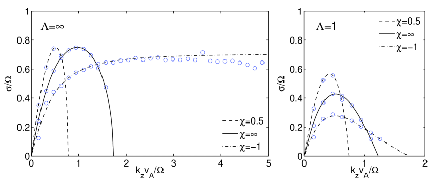
We adopt a very slim simulation box = resolved by cells, since we are interested in the vertical wave numbers. Following Sano & Stone (2002a), we initialize the problem with uniform gas density and random velocity perturbations (white noise) on the order of . We run the test simulations with given Ohmic and Hall Elsasser numbers as input parameters for about 2.5 orbits. From the simulations we perform Fourier analysis and evaluate the growth rate of for every single vertical mode from time to . In Figure 12, we show the analytical growth rate versus numerical growth rate from our test simulations. Note that the parameter adopted in Sano & Stone (2002a) corresponds to in our case. We have considered parameters with and , corresponding to and in Sano & Stone (2002a). We see that the numerical dispersion relation agrees very well with analytical results. Particularly, for , MRI growth rate is well reproduced toward very small wavelength due to the low level of intrinsic dissipation. This test demonstrates that our implementation of the Hall term is well suited for conducting simulations in the shearing-box framework.
References
- Alexiades et al. (1996) Alexiades, V., Amiez, G., & Gremaud, P. 1996, Communications in Numerical Methods in Engineering, 12, 31
- Bai (2011a) Bai, X.-N. 2011a, ApJ, 739, 50
- Bai (2011b) —. 2011b, ApJ, 739, 51
- Bai (2012) —. 2012, PhD thesis, Princeton University
- Bai (2013) —. 2013, ApJ, 772, 96
- Bai & Goodman (2009) Bai, X.-N. & Goodman, J. 2009, ApJ, 701, 737
- Bai & Stone (2010a) Bai, X.-N. & Stone, J. M. 2010a, ApJ, 722, 1437
- Bai & Stone (2010b) —. 2010b, ApJ, 722, L220
- Bai & Stone (2011) —. 2011, ApJ, 736, 144
- Bai & Stone (2013a) —. 2013a, ApJ, 767, 30
- Bai & Stone (2013b) —. 2013b, ApJ, 769, 76
- Balbus & Hawley (1991) Balbus, S. A. & Hawley, J. F. 1991, ApJ, 376, 214
- Balbus & Terquem (2001) Balbus, S. A. & Terquem, C. 2001, ApJ, 552, 235
- Birnstiel et al. (2012) Birnstiel, T., Klahr, H., & Ercolano, B. 2012, A&A, 539, A148
- Blaes & Balbus (1994) Blaes, O. M. & Balbus, S. A. 1994, ApJ, 421, 163
- Blandford & Payne (1982) Blandford, R. D. & Payne, D. G. 1982, MNRAS, 199, 883
- Chapman et al. (2013) Chapman, N. L., Davidson, J. A., Goldsmith, P. F., Houde, M., Kwon, W., Li, Z.-Y., Looney, L. W., Matthews, B., Matthews, T. G., Novak, G., Peng, R., Vaillancourt, J. E., & Volgenau, N. H. 2013, ApJ, 770, 151
- Choi et al. (2009) Choi, E., Kim, J., & Wiita, P. J. 2009, ApJS, 181, 413
- Crutcher (2012) Crutcher, R. M. 2012, ARA&A, 50, 29
- D’Alessio et al. (2006) D’Alessio, P., Calvet, N., Hartmann, L., Franco-Hernández, R., & Servín, H. 2006, ApJ, 638, 314
- Davis et al. (2010) Davis, S. W., Stone, J. M., & Pessah, M. E. 2010, ApJ, 713, 52
- Desch (2004) Desch, S. J. 2004, ApJ, 608, 509
- Dong et al. (2011) Dong, R., Rafikov, R. R., & Stone, J. M. 2011, ApJ, 741, 57
- Ercolano & Glassgold (2013) Ercolano, B. & Glassgold, A. E. 2013, MNRAS, 436, 3446
- Falle (2003) Falle, S. A. E. G. 2003, MNRAS, 344, 1210
- Ferreira & Pelletier (1995) Ferreira, J. & Pelletier, G. 1995, A&A, 295, 807
- Fleming & Stone (2003) Fleming, T. & Stone, J. M. 2003, ApJ, 585, 908
- Fleming et al. (2000) Fleming, T. P., Stone, J. M., & Hawley, J. F. 2000, ApJ, 530, 464
- Fromang et al. (2013) Fromang, S., Latter, H., Lesur, G., & Ogilvie, G. I. 2013, A&A, 552, A71
- Fromang et al. (2002) Fromang, S., Terquem, C., & Balbus, S. A. 2002, MNRAS, 329, 18
- Gammie (1996) Gammie, C. F. 1996, ApJ, 457, 355
- Garaud (2007) Garaud, P. 2007, ApJ, 671, 2091
- Gardiner & Stone (2005) Gardiner, T. A. & Stone, J. M. 2005, Journal of Computational Physics, 205, 509
- Gardiner & Stone (2008) —. 2008, Journal of Computational Physics, 227, 4123
- Goldreich & Lynden-Bell (1965) Goldreich, P. & Lynden-Bell, D. 1965, MNRAS, 130, 125
- Goodman & Rafikov (2001) Goodman, J. & Rafikov, R. R. 2001, ApJ, 552, 793
- Gressel et al. (2013) Gressel, O., Nelson, R. P., Turner, N. J., & Ziegler, U. 2013, ApJ, 779, 59
- Guilet & Ogilvie (2012) Guilet, J. & Ogilvie, G. I. 2012, MNRAS, 424, 2097
- Guilet & Ogilvie (2013) —. 2013, MNRAS, 430, 822
- Hartmann et al. (1998) Hartmann, L., Calvet, N., Gullbring, E., & D’Alessio, P. 1998, ApJ, 495, 385
- Hayashi (1981) Hayashi, C. 1981, Progress of Theoretical Physics Supplement, 70, 35
- Hennebelle & Ciardi (2009) Hennebelle, P. & Ciardi, A. 2009, A&A, 506, L29
- Hirose & Turner (2011) Hirose, S. & Turner, N. J. 2011, ApJ, 732, L30
- Hughes & Armitage (2012) Hughes, A. L. H. & Armitage, P. J. 2012, MNRAS, 423, 389
- Hull et al. (2014) Hull, C. L. H., Plambeck, R. L., Kwon, W., Bower, G. C., Carpenter, J. M., Crutcher, R. M., Fiege, J. D., Franzmann, E., Hakobian, N. S., Heiles, C., Houde, M., Hughes, A. M., Lamb, J. W., Looney, L. W., Marrone, D. P., Matthews, B. C., Pillai, T., Pound, M. W., Rahman, N., Sandell, G., Stephens, I. W., Tobin, J. J., Vaillancourt, J. E., Volgenau, N. H., & Wright, M. C. H. 2014, ApJ, submitted
- Ida et al. (2008) Ida, S., Guillot, T., & Morbidelli, A. 2008, ApJ, 686, 1292
- Igea & Glassgold (1999) Igea, J. & Glassgold, A. E. 1999, ApJ, 518, 848
- Ilgner & Nelson (2006) Ilgner, M. & Nelson, R. P. 2006, A&A, 445, 205
- Jin (1996) Jin, L. 1996, ApJ, 457, 798
- Johansen et al. (2009) Johansen, A., Youdin, A., & Mac Low, M. 2009, ApJ, 704, L75
- Joos et al. (2012) Joos, M., Hennebelle, P., & Ciardi, A. 2012, A&A, 543, A128
- Klahr & Hubbard (2014) Klahr, H. & Hubbard, A. 2014, ApJ, 788, 21
- Kley & Nelson (2012) Kley, W. & Nelson, R. P. 2012, ARA&A, 50
- Königl et al. (2010) Königl, A., Salmeron, R., & Wardle, M. 2010, MNRAS, 401, 479
- Krasnopolsky et al. (2011) Krasnopolsky, R., Li, Z.-Y., & Shang, H. 2011, ApJ, 733, 54
- Kretke & Lin (2012) Kretke, K. A. & Lin, D. N. C. 2012, ApJ, 755, 74
- Kretke et al. (2009) Kretke, K. A., Lin, D. N. C., Garaud, P., & Turner, N. J. 2009, ApJ, 690, 407
- Kunz (2008) Kunz, M. W. 2008, MNRAS, 385, 1494
- Kunz & Balbus (2004) Kunz, M. W. & Balbus, S. A. 2004, MNRAS, 348, 355
- Kunz & Lesur (2013) Kunz, M. W. & Lesur, G. 2013, MNRAS, 434, 2295
- Kunz et al. (2014) Kunz, M. W., Stone, J. M., & Bai, X.-N. 2014, Journal of Computational Physics, arXiv:1311.4865
- Latter & Balbus (2012) Latter, H. N. & Balbus, S. 2012, MNRAS, 424, 1977
- Latter et al. (2010) Latter, H. N., Fromang, S., & Gressel, O. 2010, MNRAS, 406, 848
- Lesur et al. (2013) Lesur, G., Ferreira, J., & Ogilvie, G. I. 2013, A&A, 550, A61
- Lesur et al. (2014) Lesur, G., Kunz, M. W., & Fromang, S. 2014, ArXiv e-prints
- Lesur & Papaloizou (2010) Lesur, G. & Papaloizou, J. C. B. 2010, A&A, 513, A60
- Li (1996) Li, Z.-Y. 1996, ApJ, 465, 855
- Li et al. (2011) Li, Z.-Y., Krasnopolsky, R., & Shang, H. 2011, ApJ, 738, 180
- Lovelace et al. (1999) Lovelace, R. V. E., Li, H., Colgate, S. A., & Nelson, A. F. 1999, ApJ, 513, 805
- Lubow et al. (1994) Lubow, S. H., Papaloizou, J. C. B., & Pringle, J. E. 1994, MNRAS, 268, 1010
- Lyra (2014) Lyra, W. 2014, ArXiv e-prints
- Lyra & Klahr (2011) Lyra, W. & Klahr, H. 2011, A&A, 527, A138
- Marcus et al. (2013) Marcus, P. S., Pei, S., Jiang, C.-H., & Hassanzadeh, P. 2013, Physical Review Letters, 111, 084501
- McElroy et al. (2013) McElroy, D., Walsh, C., Markwick, A. J., Cordiner, M. A., Smith, K., & Millar, T. J. 2013, A&A, arXiv:1212.6362
- Mellon & Li (2008) Mellon, R. R. & Li, Z.-Y. 2008, ApJ, 681, 1356
- Miyoshi & Kusano (2005) Miyoshi, T. & Kusano, K. 2005, Journal of Computational Physics, 208, 315
- Nelson & Gressel (2010) Nelson, R. P. & Gressel, O. 2010, MNRAS, 409, 639
- Nelson et al. (2013) Nelson, R. P., Gressel, O., & Umurhan, O. M. 2013, MNRAS, 435, 2610
- Okuzumi & Hirose (2011) Okuzumi, S. & Hirose, S. 2011, ApJ, 742, 65
- Okuzumi et al. (2013) Okuzumi, S., Takeuchi, T., & Muto, T. 2013, ArXiv e-prints
- Ormel & Okuzumi (2013) Ormel, C. W. & Okuzumi, S. 2013, ApJ, 771, 44
- O’Sullivan & Downes (2006) O’Sullivan, S. & Downes, T. P. 2006, MNRAS, 366, 1329
- O’Sullivan & Downes (2007) —. 2007, MNRAS, 376, 1648
- Paardekooper et al. (2011) Paardekooper, S.-J., Baruteau, C., & Kley, W. 2011, MNRAS, 410, 293
- Perez-Becker & Chiang (2011a) Perez-Becker, D. & Chiang, E. 2011a, ApJ, 735, 8
- Perez-Becker & Chiang (2011b) —. 2011b, ApJ, 727, 2
- Petersen et al. (2007) Petersen, M. R., Stewart, G. R., & Julien, K. 2007, ApJ, 658, 1252
- Pinilla et al. (2012) Pinilla, P., Birnstiel, T., Ricci, L., Dullemond, C. P., Uribe, A. L., Testi, L., & Natta, A. 2012, A&A, 538, A114
- Preibisch et al. (2005) Preibisch, T., Kim, Y., Favata, F., Feigelson, E. D., Flaccomio, E., Getman, K., Micela, G., Sciortino, S., Stassun, K., Stelzer, B., & Zinnecker, H. 2005, ApJS, 160, 401
- Raettig et al. (2013) Raettig, N., Lyra, W., & Klahr, H. 2013, ApJ, 765, 115
- Ribas et al. (2013) Ribas, Á., Merín, B., Bouy, H., & Maud, L. T. 2013, ArXiv e-prints
- Salmeron et al. (2011) Salmeron, R., Königl, A., & Wardle, M. 2011, MNRAS, 412, 1162
- Sano & Miyama (1999) Sano, T. & Miyama, S. M. 1999, ApJ, 515, 776
- Sano et al. (2000) Sano, T., Miyama, S. M., Umebayashi, T., & Nakano, T. 2000, ApJ, 543, 486
- Sano & Stone (2002a) Sano, T. & Stone, J. M. 2002a, ApJ, 570, 314
- Sano & Stone (2002b) —. 2002b, ApJ, 577, 534
- Santos-Lima et al. (2012) Santos-Lima, R., de Gouveia Dal Pino, E. M., & Lazarian, A. 2012, ApJ, 747, 21
- Seifried et al. (2012) Seifried, D., Banerjee, R., Pudritz, R. E., & Klessen, R. S. 2012, MNRAS, 423, L40
- Shakura & Sunyaev (1973) Shakura, N. I. & Sunyaev, R. A. 1973, A&A, 24, 337
- Sicilia-Aguilar et al. (2006) Sicilia-Aguilar, A., Hartmann, L., Calvet, N., Megeath, S. T., Muzerolle, J., Allen, L., D’Alessio, P., Merín, B., Stauffer, J., Young, E., & Lada, C. 2006, ApJ, 638, 897
- Simon et al. (2013a) Simon, J. B., Bai, X.-N., Armitage, P. J., Stone, J. M., & Beckwith, K. 2013a, ApJ, 775, 73
- Simon et al. (2013b) Simon, J. B., Bai, X.-N., Stone, J. M., Armitage, P. J., & Beckwith, K. 2013b, ApJ, 764, 66
- Stapelfeldt et al. (2003) Stapelfeldt, K. R., Ménard, F., Watson, A. M., Krist, J. E., Dougados, C., Padgett, D. L., & Brandner, W. 2003, ApJ, 589, 410
- Stone & Gardiner (2010) Stone, J. M. & Gardiner, T. A. 2010, ApJS, 189, 142
- Stone et al. (2008) Stone, J. M., Gardiner, T. A., Teuben, P., Hawley, J. F., & Simon, J. B. 2008, ApJS, 178, 137
- Suzuki & Inutsuka (2009) Suzuki, T. K. & Inutsuka, S.-i. 2009, ApJ, 691, L49
- Suzuki & Inutsuka (2014) —. 2014, ApJ, 784, 121
- Takeuchi & Okuzumi (2013) Takeuchi, T. & Okuzumi, S. 2013, ArXiv e-prints
- Tomida et al. (2013) Tomida, K., Tomisaka, K., Matsumoto, T., Hori, Y., Okuzumi, S., Machida, M. N., & Saigo, K. 2013, ApJ, 763, 6
- Tóth et al. (2008) Tóth, G., Ma, Y., & Gombosi, T. I. 2008, Journal of Computational Physics, 227, 6967
- Turner et al. (2014) Turner, N. J., Fromang, S., Gammie, C. F., Lesur, G., Wardle, M., & Bai, X.-N. 2014, in PPVI, ed. C. P. Dullemond No. arXiv:1401.7306
- Turner & Sano (2008) Turner, N. J. & Sano, T. 2008, ApJ, 679, L131
- Urpin (2003) Urpin, V. 2003, A&A, 404, 397
- Varnière & Tagger (2006) Varnière, P. & Tagger, M. 2006, A&A, 446, L13
- Walsh et al. (2010) Walsh, C., Millar, T. J., & Nomura, H. 2010, ApJ, 722, 1607
- Walsh et al. (2012) Walsh, C., Nomura, H., Millar, T. J., & Aikawa, Y. 2012, ApJ, 747, 114
- Wardle (1997) Wardle, M. 1997, in Astronomical Society of the Pacific Conference Series, Vol. 121, IAU Colloq. 163: Accretion Phenomena and Related Outflows, ed. D. T. Wickramasinghe, G. V. Bicknell, & L. Ferrario, 561
- Wardle (1999) Wardle, M. 1999, MNRAS, 307, 849
- Wardle (2007) —. 2007, Ap&SS, 311, 35
- Wardle & Koenigl (1993) Wardle, M. & Koenigl, A. 1993, ApJ, 410, 218
- Wardle & Salmeron (2012) Wardle, M. & Salmeron, R. 2012, MNRAS, 422, 2737
- Weidenschilling (1977) Weidenschilling, S. J. 1977, MNRAS, 180, 57
- Wolk et al. (2005) Wolk, S. J., Harnden, Jr., F. R., Flaccomio, E., Micela, G., Favata, F., Shang, H., & Feigelson, E. D. 2005, ApJS, 160, 423
- Yang et al. (2012) Yang, C.-C., Mac Low, M.-M., & Menou, K. 2012, ApJ, 748, 79
- Youdin (2011) Youdin, A. N. 2011, ApJ, 731, 99