Dispersive approach to hadronic light-by-light scattering

Abstract

Based on dispersion theory, we present a formalism for a model-independent evaluation of the hadronic light-by-light contribution to the anomalous magnetic moment of the muon. In particular, we comment on the definition of the pion pole in this framework and provide a master formula that relates the effect from $\pi\pi$ intermediate states to the partial waves for the process $\gamma^{*}\gamma^{*}\to\pi\pi$. All contributions are expressed in terms of on-shell form factors and scattering amplitudes, and as such amenable to an experimental determination.

Albert Einstein Center for Fundamental Physics, Institute for Theoretical Physics,
University of Bern, Sidlerstrasse 5, CH–3012 Bern, Switzerland

1 Introduction

Hadronic contributions dominate the uncertainty in the Standard-Model prediction of the anomalous magnetic moment of the muon $a_{\mu}=(g-2)_{\mu}/2$, see e.g. [1, 2]. In view of the next round of $(g-2)_{\mu}$ experiments at FNAL and J-PARC aimed at reducing the experimental error by a factor of $4$, control over these hadronic effects has to be improved substantially to make sure that experiment and Standard-Model prediction continue to compete at the same accuracy.

The leading hadronic contribution, hadronic vacuum polarization (HVP), can be related directly to the total hadronic cross section in $e^{+}e^{-}$ scattering and, given a dedicated $e^{+}e^{-}$ program, it is expected to allow for the required improvement, see e.g. [3]. In contrast, the subleading hadronic light-by-light (HLbL) scattering contribution has so far been evaluated within hadronic models and frameworks that partially incorporate rigorous constraints from QCD [7, 8, 9, 10, 11, 12, 13, 14, 15, 16, 17, 18]. In this context, a reliable estimate of the uncertainty associated with HLbL scattering as well as future reductions thereof appear difficult. As an alternative, model-independent approach to the problem, lattice QCD calculations have been proposed [19], but it is yet premature to make predictions about when such calculations will become competitive (for the present status see [20, 3]). Accordingly, HLbL scattering will soon dominate the theory error and thus become the roadblock in fully exploiting the new $(g-2)_{\mu}$ measurements.

Here, we propose to use dispersion theory to analyze HLbL scattering, similarly to what is done for HVP. In this framework, the amplitude is characterized by its analytic structure, i.e. poles and cuts, so that the relevant quantities are residues and imaginary parts, and thus, by definition, on-shell form factors and scattering amplitudes. In this way, a direct correspondence to experimentally accessible quantities can ultimately be established. While the advantages are evident, such an approach has been long sought after. However, due to the more complicated structure of HLbL scattering, it has not been possible so far to write down a formula strictly analogous to that for HVP that includes all possible hadronic intermediate states. In the present paper we make the first step in that direction, based on the assumption that the most important contributions are due to the single- and double-pion intermediate states. While the former has been analyzed in several papers in a (to a large extent) model-independent way, this is not the case for the latter. The main novelty of this paper is a master formula that explicitly relates the contribution of two-pion intermediate states to $a_{\mu}$ to the partial waves for $\gamma^{*}\gamma^{*}\to\pi\pi$. In particular, within our framework the issues raised in [21, 22, 23] concerning the dressing of the pion loop can be settled with input from experiment.

The outline of the paper is as follows: in Sect. 2 we introduce our dispersive approach, we illustrate it using the example of the pion pole, commenting on its definition within this picture, and then collect the necessary notation concerning $\gamma^{*}\gamma^{*}\to\pi\pi$ partial waves which will later be needed for the analysis of $\pi\pi$ intermediate states. In Sect. 3, we derive a set of dispersion relations for HLbL scattering, leading to an expression for the $\pi\pi$ contribution to $a_{\mu}$ in terms of $\gamma^{*}\gamma^{*}\to\pi\pi$ partial waves. Finally, we offer our conclusions and an outlook in Sect. 4. Various details of the calculation are discussed in the appendices.

2 Dispersive framework for hadronic light-by-light scattering

2.1 Notation

We define the HLbL tensor $\Pi^{\mu\nu\lambda\sigma}$ as

$$\Pi^{\mu\nu\lambda\sigma}\big{(}q_{1},q_{2},q_{3}\big{)}=i^{3}\int d^{4}x\int d^{4}y\int d^{4}z\,e^{-i(x\cdot q_{1}+y\cdot q_{2}+z\cdot q_{3})}\langle 0|T\big{\{}j^{\mu}(x)j^{\nu}(y)j^{\lambda}(z)j^{\sigma}(0)\big{\}}|0\rangle,$$ (2.1)

where $j^{\mu}(x)=\sum_{i}Q_{i}\bar{q}_{i}(x)\gamma^{\mu}q_{i}(x)$, $i=u,d,s$, is the electromagnetic current ($Q_{i}$ being the charge of the quark in proton charge units) and the matrix element is to be evaluated in pure QCD (i.e. for $\alpha=e^{2}/(4\pi)=0$). In the calculation of $a_{\mu}$ we take the external photon to couple with the fourth current, and denote its momentum by $k=q_{1}+q_{2}+q_{3}$. In addition, we need the above tensor in the kinematic configuration $k^{2}=0$. Contracted with the appropriate polarization vectors this gives the matrix element of the leading-order (in $\alpha$) hadronic contribution to the reaction

$$H_{\lambda_{1}\lambda_{2},\lambda_{3}\lambda_{4}}(s,t,u) \equiv\mathcal{M}(\gamma^{*}(q_{1},\lambda_{1})\gamma^{*}(q_{2},\lambda_{2})\to\gamma^{*}(-q_{3},\lambda_{3})\gamma(k,\lambda_{4}))$$

$$=\epsilon_{\mu}(\lambda_{1},q_{1})\epsilon_{\nu}(\lambda_{2},q_{2})\epsilon^{*}_{\lambda}(\lambda_{3},-q_{3})\epsilon^{*}_{\sigma}(\lambda_{4},k)\Pi^{\mu\nu\lambda\sigma}(q_{1},q_{2},q_{3}),$$ (2.2)

with Mandelstam variables

$$s=(q_{1}+q_{2})^{2}=(k-q_{3})^{2},\qquad t=(q_{1}+q_{3})^{2}=(k-q_{2})^{2},\qquad u=(q_{2}+q_{3})^{2}=(k-q_{1})^{2},$$ (2.3)

and $s$-channel scattering angle

$$z_{s}=\cos\theta_{s}=\frac{s}{\big{(}s-q_{3}^{2}\big{)}\sqrt{\lambda_{12}}}\bigg{(}t-u+\frac{\big{(}q_{1}^{2}-q_{2}^{2}\big{)}q_{3}^{2}}{s}\bigg{)},\qquad\lambda_{12}=\lambda\big{(}s,q_{1}^{2},q_{2}^{2}\big{)},$$ (2.4)

with $\lambda(x,y,z)=x^{2}+y^{2}+z^{2}-2(xy+xz+yz)$ the Källén function. For the contribution to $a_{\mu}$ we only need the derivative with respect to the external photon momentum $k^{\sigma}$, since by virtue of gauge invariance [24]

$$\Pi_{\mu\nu\lambda\sigma}\big{(}q_{1},q_{2},k-q_{1}-q_{2}\big{)}=-k^{\rho}\frac{\partial}{\partial k^{\sigma}}\Pi_{\mu\nu\lambda\rho}\big{(}q_{1},q_{2},k-q_{1}-q_{2}\big{)}.$$ (2.5)

The contribution to $a_{\mu}$ follows from

$$a_{\mu} =\lim_{k\to 0}\text{Tr}\Big{\{}\big{(}\not{p}+m\big{)}\Lambda^{\rho}\big{(}p^{\prime},p\big{)}\big{(}\not{p}^{\prime}+m\big{)}\Gamma_{\rho}\big{(}p^{\prime},p\big{)}\Big{\}},$$

$$\Gamma_{\rho}\big{(}p^{\prime},p\big{)} =e^{6}\int\frac{\text{d}^{4}q_{1}}{(2\pi)^{4}}\int\frac{\text{d}^{4}q_{2}}{(2\pi)^{4}}\frac{1}{q_{1}^{2}q_{2}^{2}q_{3}^{2}}\frac{\gamma^{\mu}\big{(}\not{p}^{\prime}+\not{q_{1}}+m\big{)}\gamma^{\lambda}\big{(}\not{p}-\not{q_{2}}+m)\gamma^{\nu}}{\big{(}(p^{\prime}+q_{1})^{2}-m^{2}\big{)}\big{(}(p-q_{2})^{2}-m^{2}\big{)}}k^{\sigma}\frac{\partial}{\partial k^{\rho}}\Pi_{\mu\nu\lambda\sigma},$$ (2.6)

with the projector [25]

$$\Lambda^{\rho}\big{(}p^{\prime},p\big{)}=\frac{m^{2}}{k^{2}\big{(}4m^{2}-k^{2}\big{)}}\Bigg{\{}\gamma^{\rho}+\frac{k^{2}+2m^{2}}{m\big{(}k^{2}-4m^{2}\big{)}}\big{(}p+p^{\prime}\big{)}^{\rho}\Bigg{\}}.$$ (2.7)

$m$ denotes the mass of the muon, $p$ and $p^{\prime}=p-k$ the momenta of the incoming and outgoing muon, respectively, and we have assumed that $\Pi_{\mu\nu\lambda\sigma}$ is already manifestly gauge invariant and crossing symmetric. The general relation (2.1) can be further simplified using the identity

$$\big{(}\not{p}+m\big{)}\gamma^{\rho}\big{(}\not{p}^{\prime}+m\big{)}=\big{(}\not{p}+m\big{)}\bigg{[}\frac{1}{2m}\big{(}p+p^{\prime}\big{)}^{\rho}+\frac{i}{2m}\sigma^{\rho\tau}k_{\tau}\bigg{]}\big{(}\not{p}^{\prime}+m\big{)}.$$ (2.8)

Explicit expressions will be given in (2.3) and (F.1).

2.2 Layout of the dispersive approach

In a dispersive approach one exploits the analytic properties of the matrix element of interest and reconstructs it completely from information on its analytic singularities: residues of poles, values along cuts, and subtraction constants (representing singularities at infinity). Depending on the complexity of the singularity structure of a given amplitude such a program can be carried out until the very end (as in the case of form factors), or lead to integral equations amenable to numerical treatment. In the worst case the singularity structure may be too complex to allow for an exact treatment. The HLbL amplitude clearly belongs to the latter class, unfortunately: it has single poles, cuts in all channels (and simultaneously in different channels), and in all photon momenta squared, as well as anomalous thresholds [26, 27, 28].

$F_{\pi}^{V}\big{(}q_{1}^{2}\big{)}F_{\pi}^{V}\big{(}q_{2}^{2}\big{)}F_{\pi}^{V}\big{(}q_{3}^{2}\big{)}\times\left[\hskip 5.69046pt\raisebox{-46.94687pt}{ \includegraphics[width=86.72267pt]{box_cut_sQED_solid} \quad\includegraphics[width=86.72267pt]{triangle_cut_sQED_solid} \quad\raisebox{21.90874pt}{\includegraphics[width=86.72267pt]{bulb_cut_sQED_solid}} }\hskip 5.69046pt\right]$

Figure 1: Scalar QED diagrams with photon–pion vertices dressed by the (appropriate power of) pion vector form factors, in the following referred to as FsQED. Solid lines denote pions, wiggly lines photons, and the dashed lines indicate the cutting of the pion propagators.

On the basis of model calculations (see, e.g. [9]) of the HLbL contributions to $a_{\mu}$, it is clear that singularities having higher thresholds (like the cut due to $\bar{K}K$ intermediate states) are less important. It appears therefore reasonable to reduce the complexity of the problem by limiting ourselves to the lowest-lying intermediate states, pions, and to allow for at most two pions in intermediate states. In this approximation the HLbL tensor can be broken down into the following contributions

$$\Pi_{\mu\nu\lambda\sigma}=\Pi_{\mu\nu\lambda\sigma}^{\pi^{0}\text{-pole}}+\Pi_{\mu\nu\lambda\sigma}^{\text{FsQED}}+\bar{\Pi}_{\mu\nu\lambda\sigma}+\cdots,$$ (2.9)

where $\Pi_{\mu\nu\lambda\sigma}^{\pi^{0}\text{-pole}}$ refers to the pion pole, $\Pi_{\mu\nu\lambda\sigma}^{\text{FsQED}}$ to the amplitude in scalar QED with vertices dressed by the (appropriate power of) pion vector form factors $F_{\pi}^{V}(q^{2})$ (FsQED), $\bar{\Pi}_{\mu\nu\lambda\sigma}$ to the remaining $\pi\pi$ contribution, and the ellipsis to higher-mass poles and intermediate states.

The reason for separating the FsQED contribution from the rest and its precise meaning can be explained as follows: $\Pi_{\mu\nu\lambda\sigma}^{\text{FsQED}}$ includes the contribution due to simultaneous two-pion cuts in two of the channels (by crossing symmetry it contains three contributions with simultaneous singularities in the $(s,t)$, $(s,u)$, and $(t,u)$ channels, respectively). One first takes the two-pion cut in the $s$-channel, which gives the discontinuity as the product of two $\gamma^{*}\gamma^{*}\to\pi\pi$ amplitudes, and then selects the Born term (the pure pole term) in each of the two amplitudes, as illustrated by the leftmost diagram in Fig. 1. The singularity of this diagram is therefore given by four $\pi^{+}\pi^{-}\gamma^{*}$ vertices with on-shell pions—which implies that these vertices are nothing but the full pion vector form factors. On the other hand, the singularity structure of this contribution is identical to that of a Feynman box diagram with four pion propagators: since the four vertices depend only on the momentum squared of the external photons and on none of the internal momenta, this contribution is given by the box-diagram multiplied by three pion vector form factors (since one of the photons is on-shell). In sQED the box diagram in Fig. 1 is not gauge invariant on its own, however. The photon–scalar–scalar vertex comes together with the seagull term (two-photon–two-scalar vertex), with couplings strictly related to each other: in any amplitude with two or more photons both vertices have to be taken into account to form a subset of gauge-invariant diagrams. Therefore, in sQED the box diagram has to be accompanied by a triangle and a bulb diagram in order to respect gauge invariance, as shown in Fig. 1. We do the same here and define our gauge-invariant box diagram as the charged pion loop calculated within sQED multiplied by the pion vector form factors.

We stress that the separation of this contribution from the rest is unambiguous as it is based on its analytic properties, namely the presence of simultaneous cuts in two channels. The request to have the two simultaneous cuts is equivalent to putting all pions in the box diagram on-shell, but does not put constraints on the vertex with the photon, which is allowed to have its full $q^{2}$-dependence. The fact that the two pions in the vertex are both on-shell, however, allows us to identify that vertex with the pion vector form factor: multiplying the sQED contribution by three pion form factors, as shown in Fig. 1, is not an approximation, but the exact and unambiguous representation of the contribution with these analytic properties. How to technically separate this contribution from the others with two-pion intermediate states and how they contribute to $a_{\mu}$ will be discussed in more detail in Sect. 3.4.

Since we only explicitly consider cuts from up to two-pion intermediate states, this implies that the analytic structure of the remainder $\bar{\Pi}_{\mu\nu\lambda\sigma}$ in (2.9) does not involve so-called double-spectral regions, i.e. parts of the Mandelstam plane with simultaneous singularities in two Mandelstam variables, and can therefore be expanded in partial waves, making a dispersive treatment of this part feasible. In the rest of this section we first specify the contribution of the pion pole to $a_{\mu}$, and then set up the notation for the $\gamma^{*}\gamma^{*}\to\pi\pi$ reaction. Based on these conventions, we will derive dispersion relations for $\bar{\Pi}_{\mu\nu\lambda\sigma}$ in Sect. 3.

2.3 Pion pole

The dominant contribution to HLbL scattering at low energy is given by the $\pi^{0}$-poles. Their residues are determined by the on-shell, doubly-virtual pion transition form factor $\mathcal{F}_{\pi^{0}\gamma^{*}\gamma^{*}}(q_{1}^{2},q_{2}^{2})$, which is defined as the current matrix element

$$i\int\text{d}^{4}x\,e^{iq\cdot x}\big{\langle}0\big{|}T\big{\{}j_{\mu}(x)j_{\nu}(0)\big{\}}\big{|}\pi^{0}(p)\big{\rangle}=\epsilon_{\mu\nu\alpha\beta}q^{\alpha}p^{\beta}\mathcal{F}_{\pi^{0}\gamma^{*}\gamma^{*}}\big{(}q^{2},(p-q)^{2}\big{)}.$$ (2.10)

In these conventions, the $\pi^{0}$-pole HLbL amplitude reads

$$\Pi_{\mu\nu\lambda\sigma}^{\pi^{0}\text{-pole}} =\frac{\mathcal{F}_{\pi^{0}\gamma^{*}\gamma^{*}}\big{(}q_{1}^{2},q_{2}^{2}\big{)}\mathcal{F}_{\pi^{0}\gamma^{*}\gamma^{*}}\big{(}q_{3}^{2},0\big{)}}{s-M_{\pi^{0}}^{2}}\epsilon_{\mu\nu\alpha\beta}q_{1}^{\alpha}q_{2}^{\beta}\epsilon_{\lambda\sigma\gamma\delta}q_{3}^{\gamma}k^{\delta}$$

$$+\frac{\mathcal{F}_{\pi^{0}\gamma^{*}\gamma^{*}}\big{(}q_{1}^{2},q_{3}^{2}\big{)}\mathcal{F}_{\pi^{0}\gamma^{*}\gamma^{*}}\big{(}q_{2}^{2},0\big{)}}{t-M_{\pi^{0}}^{2}}\epsilon_{\mu\lambda\alpha\beta}q_{1}^{\alpha}q_{3}^{\beta}\epsilon_{\nu\sigma\gamma\delta}q_{2}^{\gamma}k^{\delta}$$

$$+\frac{\mathcal{F}_{\pi^{0}\gamma^{*}\gamma^{*}}\big{(}q_{2}^{2},q_{3}^{2}\big{)}\mathcal{F}_{\pi^{0}\gamma^{*}\gamma^{*}}\big{(}q_{1}^{2},0\big{)}}{u-M_{\pi^{0}}^{2}}\epsilon_{\nu\lambda\alpha\beta}q_{2}^{\alpha}q_{3}^{\beta}\epsilon_{\mu\sigma\gamma\delta}q_{1}^{\gamma}k^{\delta}.$$ (2.11)

Its contribution to $a_{\mu}$ can be derived from

$$a_{\mu} =\frac{1}{48m}\text{Tr}\Big{\{}\big{(}\not{p}+m\big{)}\big{[}\gamma^{\rho},\gamma^{\sigma}\big{]}\big{(}\not{p}+m\big{)}\Gamma_{\rho\sigma}\Big{\}},$$

$$\Gamma_{\rho\sigma} =-e^{6}\int\frac{\text{d}^{4}q_{1}}{(2\pi)^{4}}\int\frac{\text{d}^{4}q_{2}}{(2\pi)^{4}}\frac{1}{q_{1}^{2}q_{2}^{2}s}\frac{\gamma^{\mu}\big{(}\not{p}+\not{q_{1}}+m\big{)}\gamma^{\lambda}\big{(}\not{p}-\not{q_{2}}+m)\gamma^{\nu}}{\big{(}(p+q_{1})^{2}-m^{2}\big{)}\big{(}(p-q_{2})^{2}-m^{2}\big{)}}\bigg{[}\frac{\partial}{\partial k^{\rho}}\Pi_{\mu\nu\lambda\sigma}\bigg{]}_{k=0}.$$ (2.12)

This formula holds true if the derivative has a well-defined limit for $k\to 0$, a condition fulfilled by the $\pi^{0}$-pole amplitude (2.3). It follows from (2.1) by averaging over the spatial directions of $k$, see [29, 30, 31], whereupon the limit may be pulled inside the integral. The final result can be expressed as [15]

$$a_{\mu}^{\pi^{0}\text{-pole}} =-e^{6}\int\frac{\text{d}^{4}q_{1}}{(2\pi)^{4}}\int\frac{\text{d}^{4}q_{2}}{(2\pi)^{4}}\frac{1}{q_{1}^{2}q_{2}^{2}s\big{(}(p+q_{1})^{2}-m^{2}\big{)}\big{(}(p-q_{2})^{2}-m^{2}\big{)}}$$ (2.13)

$$\times\Bigg{\{}\frac{\mathcal{F}_{\pi^{0}\gamma^{*}\gamma^{*}}\big{(}q_{1}^{2},q_{2}^{2}\big{)}\mathcal{F}_{\pi^{0}\gamma^{*}\gamma^{*}}\big{(}s,0\big{)}}{s-M_{\pi^{0}}^{2}}T_{1}(q_{1},q_{2};p)+\frac{\mathcal{F}_{\pi^{0}\gamma^{*}\gamma^{*}}\big{(}s,q_{2}^{2}\big{)}\mathcal{F}_{\pi^{0}\gamma^{*}\gamma^{*}}\big{(}q_{1}^{2},0\big{)}}{q_{1}^{2}-M_{\pi^{0}}^{2}}T_{2}(q_{1},q_{2};p)\Bigg{\}},$$

with

$$T_{1}(q_{1},q_{2};p) =\frac{8}{3}\bigg{\{}2p\cdot q_{1}\,p\cdot q_{2}\,q_{1}\cdot q_{2}+p\cdot q_{1}\,q_{2}^{2}\Big{(}q_{1}\cdot q_{2}+q_{1}^{2}-2p\cdot q_{1}\Big{)}-\frac{m^{2}\lambda_{12}}{4}\bigg{\}},$$ (2.14)

$$T_{2}(q_{1},q_{2};p) =\frac{16}{3}\bigg{\{}p\cdot q_{1}\Big{(}p\cdot q_{2}\,q_{1}\cdot q_{2}-p\cdot q_{1}\,q_{2}^{2}+(q_{1}\cdot q_{2})^{2}\Big{)}-\frac{q_{1}^{2}}{2}\Big{(}3p\cdot q_{1}\,q_{2}^{2}-p\cdot q_{2}\,q_{1}\cdot q_{2}\Big{)}-\frac{m^{2}\lambda_{12}}{4}\bigg{\}}.$$

Due to the $q_{1}\leftrightarrow-q_{2}$ symmetry of the integrand, the $t$- and $u$-channel terms give the same contribution.

We stress that in our dispersive framework the analytic structure of the HLbL tensor has to be analyzed for the full four-point function, i.e. with $k^{2}=0$ but otherwise general $k$. In this setting $s$ and $q_{3}^{2}$ are independent variables and the pion-pole contribution to the HLbL tensor is unambiguously given by (2.3), which leads to the result in (2.13). Within our formalism, the pion pole defined in this manner (2.13) is therefore unique.

In [17] it was pointed out that the pion-pole contribution as defined in (2.3) goes faster to zero for large $q^{2}$ than what is required by perturbative QCD, thereby becoming sub-dominant in that regime. As a cure to this problem, it was proposed in [17] to replace the singly-virtual form factor by a constant, arguing that in this way one obtains an expression which correctly interpolates between high and low $q^{2}$. As stated in that paper, the transition $\mathcal{F}_{\pi^{0}\gamma^{*}\gamma^{*}}(q^{2},0)\to{\it const}$ for large $q^{2}$ is generated by the exchange of heavier pseudoscalar resonances, which we are explicitly neglecting here. We are well aware that restoring the correct high-energy behavior has a non-negligible impact in the numerical estimate of the HLbL contribution to $a_{\mu}$. Therefore, enforcing additional short-distance constraints onto our representation is indeed a direction for future improvements of the formalism [32]. This statement pertains not only to the pion pole, but to a dispersive approach in general: with a limited number of intermediate states explicitly taken into account, the representation will be adequate at low and intermediate energies, while the correct high-energy behavior has to be enforced in a second step.

We also observe that the leading and subleading logarithmic contributions to $a_{\mu}$ in a chiral and $1/N_{C}$ expansion discussed in [16] are automatically reproduced in this approach: the leading one by construction, and the subleading one provided the measured decays $\eta\to\mu^{+}\mu^{-}$ and $\pi^{0}\to e^{+}e^{-}$ are used to constrain the off-shell dependence in $\mathcal{F}_{\pi^{0}\gamma^{*}\gamma^{*}}\big{(}q_{1}^{2},q_{2}^{2}\big{)}$.

We conclude with a brief comment about an alternative, model-dependent implementation of the pole amplitude in which the pion transition form factor is generalized to arbitrary pion virtualities [1], e.g. $\mathcal{F}_{\pi^{0}\gamma^{*}\gamma^{*}}(s,s,0)$ for the $s$-channel pole (the first argument referring to the pion virtuality). When expanded around the pole mass, any offshell-dependence from the form factors yields a polynomial contribution, as long as it does not entail more complicated analytic structure (and thus intermediate states beyond our framework). In the dispersive picture a polynomial arises if the dispersive integrals do not converge sufficiently fast and have to be subtracted. Off-shell terms calculated in a given model can be absorbed into this polynomial. Frequently, the coefficients of the subtraction polynomial are free parameters in a dispersive approach, but for HLbL scattering constraints by gauge invariance completely fix these parameters, as will be shown in Sects. 3.2 and 3.3.

2.4 Conventions for $\boldsymbol{\gamma^{*}\gamma^{*}\to\pi\pi}$

In this section we collect notation and conventions for $\gamma^{*}\gamma^{*}\to\pi\pi$. We take pion Compton scattering

$$\gamma^{*}(q_{1},\lambda_{1},\mu)\pi^{a}(p_{1})\to\gamma^{*}(q_{2},\lambda_{2},\nu)\pi^{b}(p_{2}),$$ (2.15)

with momenta, helicities, and Lorentz indices as indicated as well as isospin indices $a$, $b$ as the $s$-channel process and define Mandelstam variables according to

$$s=(q_{1}+p_{1})^{2},\qquad t=(q_{1}-q_{2})^{2},\qquad u=(q_{1}-p_{2})^{2}.$$ (2.16)

The scattering angle in the crossed channel

$$\gamma^{*}(q_{1},\lambda_{1},\mu)\gamma^{*}(-q_{2},\lambda_{2},\nu)\to\pi^{a}(-p_{1})\pi^{b}(p_{2})$$ (2.17)

is given by

$$z_{t}=\frac{s-u}{4p_{t}q_{t}},$$ (2.18)

with momenta

$$p_{t}=\sqrt{\frac{t}{4}-M_{\pi}^{2}}\equiv\frac{\sqrt{t}}{2}\sigma_{t},\qquad q_{t}=\frac{\sqrt{\lambda_{12}^{t}}}{2\sqrt{t}},\qquad\lambda_{12}^{t}=\lambda\big{(}t,q_{1}^{2},q_{2}^{2}\big{)}.$$ (2.19)

The objects of interest for HLbL scattering are the helicity amplitudes corresponding to (2.17)

$${}_{\text{out}}\langle\pi(-p_{1})\pi(p_{2})|\gamma^{*}(q_{1},\lambda_{1})\gamma^{*}(-q_{2},\lambda_{2})\rangle_{\text{in}} =ie^{2}(2\pi)^{4}\delta^{4}(q_{1}+p_{1}-q_{2}-p_{2})H_{\lambda_{1}\lambda_{2}}e^{i(\lambda_{1}-\lambda_{2})\varphi}$$

$$H_{\lambda_{1}\lambda_{2}} =\epsilon_{\mu}(q_{1},\lambda_{1})\epsilon_{\nu}(-q_{2},\lambda_{2})W^{\mu\nu},$$ (2.20)

parameterized in terms of the tensor $W^{\mu\nu}$ ($\varphi$ denotes the azimuthal angle). Its Lorentz decomposition into gauge-invariant structures that separately fulfill the Ward identities

$$q_{1}^{\mu}W_{\mu\nu}=q_{2}^{\nu}W_{\mu\nu}=0$$ (2.21)

reads

$$W_{\mu\nu}=\sum_{i=1}^{5}T_{\mu\nu}^{i}A_{i},$$ (2.22)

where

$$T^{1}_{\mu\nu} =-q_{1}\cdot q_{2}g_{\mu\nu}+q_{2\mu}q_{1\nu},$$

$$T^{2}_{\mu\nu} =-4q_{1}\cdot q_{2}\Delta_{\mu}\Delta_{\nu}-(s-u)^{2}g_{\mu\nu}+2(s-u)\big{(}\Delta_{\mu}q_{1\nu}+q_{2\mu}\Delta_{\nu}\big{)},$$

$$T^{3}_{\mu\nu} =q_{1}\cdot q_{2}q_{1\mu}q_{2\nu}+q_{1}^{2}q_{2}^{2}g_{\mu\nu}-q_{2}^{2}q_{1\mu}q_{1\nu}-q_{1}^{2}q_{2\mu}q_{2\nu},$$

$$T^{4}_{\mu\nu} =-2q_{1}\cdot q_{2}q_{1\mu}\Delta_{\nu}+2q_{1}^{2}q_{2\mu}\Delta_{\nu}-(s-u)q_{1}^{2}g_{\mu\nu}+(s-u)q_{1\mu}q_{1\nu},$$

$$T^{5}_{\mu\nu} =-2q_{1}\cdot q_{2}\Delta_{\mu}q_{2\nu}+2q_{2}^{2}\Delta_{\mu}q_{1\nu}-(s-u)q_{2}^{2}g_{\mu\nu}+(s-u)q_{2\mu}q_{2\nu},$$ (2.23)

and

$$\Delta_{\mu}=p_{1\mu}+p_{2\mu}.$$ (2.24)

To work out the explicit form of the helicity amplitudes, we choose momenta and polarization vectors as follows

$$q_{1}^{\mu} =(E_{q_{1}},0,0,q_{t}),\qquad q_{2}^{\mu}=(-E_{q_{2}},0,0,q_{t}),$$

$$p_{1}^{\mu} =(-E_{p_{1}},-p_{t}\sin\theta_{t},0,-p_{t}\cos\theta_{t}),\qquad p_{2}^{\mu}=(E_{p_{2}},-p_{t}\sin\theta_{t},0,-p_{t}\cos\theta_{t}),$$

$$\epsilon^{\mu}(q_{1},\pm) =\mp\frac{1}{\sqrt{2}}(0,1,\pm i,0),\qquad\epsilon^{\mu}(-q_{2},\pm)=\mp\frac{1}{\sqrt{2}}(0,1,\mp i,0),$$

$$\epsilon^{\mu}(q_{1},0) =\frac{1}{\xi_{1}}(q_{t},0,0,E_{q_{1}}),\qquad\epsilon^{\mu}(-q_{2},0)=\frac{1}{\xi_{2}}(-q_{t},0,0,E_{q_{2}}),$$

$$E_{q_{1}} =\frac{t+q_{1}^{2}-q_{2}^{2}}{2\sqrt{t}},\qquad E_{q_{2}}=\frac{t-q_{1}^{2}+q_{2}^{2}}{2\sqrt{t}},\qquad E_{p_{1}}=E_{p_{2}}=\frac{\sqrt{t}}{2},$$ (2.25)

leaving the normalization $\xi_{i}$ of the longitudinal polarization vectors general. In these conventions, we find the following expressions for the helicity amplitudes

$$H_{++}=H_{--} =-\frac{1}{2}\big{(}t-q_{1}^{2}-q_{2}^{2}\big{)}A_{1}+\big{(}t-4M_{\pi}^{2}\big{)}\Big{\{}\big{(}t-q_{1}^{2}-q_{2}^{2}\big{)}\big{(}1-z_{t}^{2}\big{)}+4q_{t}^{2}z_{t}^{2}\Big{\}}A_{2}-q_{1}^{2}q_{2}^{2}A_{3}$$

$$+4p_{t}q_{t}z_{t}\Big{(}q_{1}^{2}A_{4}+q_{2}^{2}A_{5}\Big{)},$$

$$H_{+-}=H_{-+} =-\big{(}t-4M_{\pi}^{2}\big{)}\big{(}t-q_{1}^{2}-q_{2}^{2}\big{)}\big{(}1-z_{t}^{2}\big{)}A_{2},$$

$$H_{+0}=-H_{-0} =\frac{q_{2}^{2}}{\xi_{2}}\bigg{[}-\big{(}t-4M_{\pi}^{2}\big{)}\sqrt{\frac{2}{t}}\big{(}t+q_{1}^{2}-q_{2}^{2}\big{)}z_{t}\sqrt{1-z_{t}^{2}}A_{2}+2p_{t}q_{t}\sqrt{2t}\sqrt{1-z_{t}^{2}}A_{5}\bigg{]},$$

$$H_{0+}=-H_{0-} =\frac{q_{1}^{2}}{\xi_{1}}\bigg{[}-\big{(}t-4M_{\pi}^{2}\big{)}\sqrt{\frac{2}{t}}\big{(}t-q_{1}^{2}+q_{2}^{2}\big{)}z_{t}\sqrt{1-z_{t}^{2}}A_{2}+2p_{t}q_{t}\sqrt{2t}\sqrt{1-z_{t}^{2}}A_{4}\bigg{]},$$

$$H_{00} =-\frac{q_{1}^{2}q_{2}^{2}}{\xi_{1}\xi_{2}}\Big{\{}A_{1}-4\big{(}t-4M_{\pi}^{2}\big{)}z_{t}^{2}A_{2}+\frac{1}{2}\big{(}t-q_{1}^{2}-q_{2}^{2}\big{)}A_{3}+4p_{t}q_{t}z_{t}\big{(}A_{4}+A_{5}\big{)}\Big{\}}.$$ (2.26)

We define the partial waves as

$$H_{++}(s,t) =\sum\limits_{J=0}^{\infty}(2J+1)P_{J}(z_{t})h_{J,++}(t),$$

$$H_{+-}(s,t) =\sum\limits_{J=2}^{\infty}(2J+1)d^{J}_{20}(z_{t})h_{J,+-}(t),$$

$$H_{+0}(s,t) =\sum\limits_{J=2}^{\infty}(2J+1)d_{10}^{J}(z_{t})h_{J,+0}(t),$$

$$H_{0+}(s,t) =\sum\limits_{J=2}^{\infty}(2J+1)d_{10}^{J}(z_{t})h_{J,0+}(t),$$

$$H_{00}(s,t) =\sum\limits_{J=0}^{\infty}(2J+1)P_{J}(z_{t})h_{J,00}(t),$$ (2.27)

where $P_{J}(z)$ denotes Legendre polynomials and $d^{J}_{mm^{\prime}}(z)$ Wigner $d$-functions, e.g.

$$d^{2}_{20}(z)=\frac{\sqrt{6}}{4}\big{(}1-z^{2}\big{)},\qquad d^{2}_{10}(z)=-\sqrt{\frac{3}{2}}z\sqrt{1-z^{2}}.$$ (2.28)

Due to Bose symmetry and invariance of strong interactions under charge conjugation, only even partial waves are allowed to contribute. $S$-waves only occur for the $++$ and $00$ projection, while all other helicity projections start at $D$-wave level. Explicit expressions for the partial-wave projections of the Born terms, $N_{J,\lambda_{1}\lambda_{2}}$, are given in App. A.

The helicity partial waves for $\gamma^{*}\gamma^{*}\to\pi\pi$ as defined in (2.4) constitute the key input for $\pi\pi$ intermediate states in the HLbL contribution to $a_{\mu}$. They fulfill important constraints known as soft-photon zeros [34, 35], which will prove crucial for the construction of dispersion relations in Sect. 3.2. The soft-photon theorem states that in the limit $q_{1}^{2}\to 0$ the Born-term-subtracted helicity amplitudes vanish if $t=q_{2}^{2}$ and vice versa. Its origin can be inferred from the decomposition (2.4). For later use it will be convenient to express these soft-photon zeros more explicitly on the level of partial waves, in the framework of partial-wave dispersion relations (see [36, 37] for the on-shell case $\gamma\gamma\to\pi\pi$ and [35] for a generalization to the singly-virtual process $\gamma^{*}\gamma\to\pi\pi$). In particular, one can derive a system of so-called Roy–Steiner equations

$$h_{J,i}(t)=\frac{1}{\pi}\sum\limits_{J^{\prime}\,\text{even}}\sum\limits_{j=1}^{5}\int\limits_{4M_{\pi}^{2}}^{\infty}\text{d}t^{\prime}K_{JJ^{\prime}}^{ij}(t,t^{\prime})\text{Im}\,h_{J^{\prime},j}(t^{\prime})+\cdots,\qquad i,j\in\big{\{}++,+-,+0,0+,00\},$$ (2.29)

where the ellipsis refers to integrals involving partial waves for $\gamma^{*}\pi\to\gamma^{*}\pi$ [37, 32]. The precise form how the soft-photon zeros manifest themselves may be read off from the diagonal kernel functions

$$K_{00}^{11}(t,t^{\prime}) =K_{00}^{55}(t,t^{\prime})=\frac{1}{t^{\prime}-t}-\frac{t^{\prime}-q_{1}^{2}-q_{2}^{2}}{\lambda_{12}^{t^{\prime}}},$$

$$K_{22}^{11}(t,t^{\prime}) =K_{22}^{55}(t,t^{\prime})=\frac{p_{t}^{2}q_{t}^{2}}{p_{t}^{\prime 2}q_{t}^{\prime 2}}\bigg{(}\frac{1}{t^{\prime}-t}-\frac{t^{\prime}-q_{1}^{2}-q_{2}^{2}}{\lambda_{12}^{t^{\prime}}}\bigg{)},$$

$$K_{22}^{22}(t,t^{\prime}) =\frac{\big{(}t-q_{1}^{2}-q_{2}^{2}\big{)}p_{t}^{2}}{(t^{\prime}-t)\big{(}t^{\prime}-q_{1}^{2}-q_{2}^{2}\big{)}p_{t}^{\prime 2}},$$

$$K_{22}^{33}(t,t^{\prime}) =K_{22}^{44}(t,t^{\prime})=\sqrt{\frac{t}{t^{\prime}}}\frac{p_{t}^{2}q_{t}^{2}}{(t^{\prime}-t)p_{t}^{\prime 2}q_{t}^{\prime 2}}.$$ (2.30)

The form of these kernel functions will be instrumental for the construction of dispersion relations for HLbL scattering in Sect. 3.2. Apart from the diagonal kernel functions (2.4) there are also non-diagonal ones, e.g. for the $S$-waves

$$K_{00}^{15}(t,t^{\prime})=\frac{2\xi_{1}\xi_{2}}{\lambda_{12}^{t^{\prime}}},\qquad K_{00}^{51}(t,t^{\prime})=\frac{2q_{1}^{2}q_{2}^{2}}{\xi_{1}\xi_{2}\lambda_{12}^{t^{\prime}}}.$$ (2.31)

The necessity of these additional kernel functions using the example of the $1$-loop amplitudes in Chiral Perturbation Theory (ChPT) is demonstrated in App. B.

3 $\boldsymbol{\pi\pi}$ intermediate states

In this section we discuss a dispersive treatment of the $\bar{\Pi}_{\mu\nu\lambda\sigma}$ part of the HLbL tensor defined in (2.9). Modifications due to the subtraction of the FsQED loop, as well as the symmetry factor for $\pi^{0}\pi^{0}$ intermediate states, will be discussed in more detail in Sect. 3.4.

The outline of the derivation is as follows: in Sect. 3.1 we first analyze the unitarity relation for $\pi\pi$ intermediate states. This leads to a set of Lorentz structures diagonal in the space of helicity amplitudes that serves as a basis for the HLbL tensor. Dispersion relations are then written down for the scalar coefficients of these Lorentz structures. The form of the diagonal kernel functions of these dispersion relations can be immediately read off from $\gamma^{*}\gamma^{*}\to\pi\pi$, as detailed in Sect. 3.2. Apart from the diagonal kernels, there are in general non-diagonal contributions, in analogy to (2.31). In Sect. 3.3 we discuss the origin of these terms and derive their explicit form for $S$-waves, before presenting our main result in Sect. 3.4.

3.1 Unitarity and decomposition of the HLbL amplitude

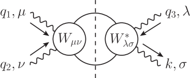
Figure 2: Unitarity relation for $\pi\pi$ intermediate states in HLbL scattering. The blobs refer to the full $\gamma^{*}\gamma^{*}\to\pi\pi$ amplitude, otherwise conventions as in Fig. 1.

We start off from the unitarity relation for $\pi\pi$ intermediate states, as illustrated in Fig. 2. The $s$-channel discontinuity of $\Pi^{\mu\nu\lambda\sigma}$ due to $\pi\pi$ intermediate states follows from

$$\text{Im}_{s}^{\pi\pi}\,\Pi_{\mu\nu\lambda\sigma} =\frac{1}{2}\int\frac{\text{d}^{3}k_{1}}{(2\pi)^{3}2E_{1}}\int\frac{\text{d}^{3}k_{2}}{(2\pi)^{3}2E_{2}}W_{\mu\nu}\big{(}\gamma^{*}(q_{1},\mu)\gamma^{*}(q_{2},\nu)\to\pi(k_{1})\pi(k_{2})\big{)}$$

$$\times W^{*}_{\lambda\sigma}\big{(}\gamma^{*}(q_{3},\lambda)\gamma(-k,\sigma)\to\pi(-k_{1})\pi(-k_{2})\big{)}(2\pi)^{4}\delta^{4}\big{(}k_{1}+k_{2}-q_{1}-q_{2}\big{)}.$$ (3.1)

The phase-space integral in (3.1) may be rewritten in terms of loop integrals

$$\text{Im}_{s}^{\pi\pi}\,\Pi^{\mu\nu\lambda\sigma} =\text{Im}_{s}\,\frac{1}{i}\int\frac{\text{d}^{4}l}{(2\pi)^{4}}\frac{1}{\big{(}l^{2}-M_{\pi}^{2}\big{)}\big{(}(l-\Sigma)^{2}-M_{\pi}^{2}\big{)}}$$ (3.2)

$$\times W_{\mu\nu}\big{(}\gamma^{*}(q_{1},\mu)\gamma^{*}(q_{2},\nu)\to\pi(l)\pi(\Sigma-l)\big{)}W^{*}_{\lambda\sigma}\big{(}\gamma^{*}(q_{3},\lambda)\gamma(-k,\sigma)\to\pi(-l)\pi(l-\Sigma)\big{)},$$

where $\Sigma=q_{1}+q_{2}$. This relation can be analyzed at a given order in a partial-wave expansion for $\gamma^{*}\gamma^{*}\to\pi\pi$ in terms of tensor integrals. Including partial waves up to $D$-waves, we find

$$\text{Im}_{s}^{\pi\pi}\,\Pi^{\mu\nu\lambda\sigma} =\frac{\sigma_{s}}{16\pi}\theta\big{(}s-4M_{\pi}^{2}\big{)}\bigg{\{}\Big{(}h_{1}\big{(}s;q_{1}^{2},q_{2}^{2}\big{)}h_{1}^{*}\big{(}s;q_{3}^{2},0\big{)}+\frac{1}{5}P_{2}(z_{s})h_{3}\big{(}s;q_{1}^{2},q_{2}^{2}\big{)}h_{3}^{*}\big{(}s;q_{3}^{2},0\big{)}\Big{)}A_{1,s}^{\mu\nu\lambda\sigma}$$

$$+\Big{(}h_{2}\big{(}s;q_{1}^{2},q_{2}^{2}\big{)}h_{1}^{*}\big{(}s;q_{3}^{2},0\big{)}+\frac{1}{5}P_{2}(z_{s})h_{7}\big{(}s;q_{1}^{2},q_{2}^{2}\big{)}h_{3}^{*}\big{(}s;q_{3}^{2},0\big{)}\Big{)}A_{2,s}^{\mu\nu\lambda\sigma}$$

$$+h_{3}\big{(}s;q_{1}^{2},q_{2}^{2}\big{)}\Big{(}h_{4}^{*}\big{(}s;q_{3}^{2},0\big{)}A_{3,s}^{\mu\nu\lambda\sigma}+h_{6}^{*}\big{(}s;q_{3}^{2},0\big{)}A_{4,s}^{\mu\nu\lambda\sigma}\Big{)}$$

$$+h_{4}\big{(}s;q_{1}^{2},q_{2}^{2}\big{)}\Big{(}h_{3}^{*}\big{(}s;q_{3}^{2},0\big{)}A_{5,s}^{\mu\nu\lambda\sigma}+h_{4}^{*}\big{(}s;q_{3}^{2},0\big{)}A_{6,s}^{\mu\nu\lambda\sigma}+h_{6}^{*}\big{(}s;q_{3}^{2},0\big{)}A_{7,s}^{\mu\nu\lambda\sigma}\Big{)}$$

$$+h_{5}\big{(}s;q_{1}^{2},q_{2}^{2}\big{)}\Big{(}h_{3}^{*}\big{(}s;q_{3}^{2},0\big{)}A_{8,s}^{\mu\nu\lambda\sigma}+h_{4}^{*}\big{(}s;q_{3}^{2},0\big{)}A_{9,s}^{\mu\nu\lambda\sigma}+h_{6}^{*}\big{(}s;q_{3}^{2},0\big{)}A_{10,s}^{\mu\nu\lambda\sigma}\Big{)}$$

$$+h_{6}\big{(}s;q_{1}^{2},q_{2}^{2}\big{)}\Big{(}h_{3}^{*}\big{(}s;q_{3}^{2},0\big{)}A_{11,s}^{\mu\nu\lambda\sigma}+h_{4}^{*}\big{(}s;q_{3}^{2},0\big{)}A_{12,s}^{\mu\nu\lambda\sigma}+h_{6}^{*}\big{(}s;q_{3}^{2},0\big{)}A_{13,s}^{\mu\nu\lambda\sigma}\Big{)}$$

$$+h_{7}\big{(}s;q_{1}^{2},q_{2}^{2}\big{)}\Big{(}h_{4}^{*}\big{(}s;q_{3}^{2},0\big{)}A_{14,s}^{\mu\nu\lambda\sigma}+h_{6}^{*}\big{(}s;q_{3}^{2},0\big{)}A_{15,s}^{\mu\nu\lambda\sigma}\Big{)}\bigg{\}},$$ (3.3)

with

$$h_{1}\big{(}s;q_{1}^{2},q_{2}^{2}\big{)} =h_{0,++}\big{(}s;q_{1}^{2},q_{2}^{2}\big{)}, h_{5}\big{(}s;q_{1}^{2},q_{2}^{2}\big{)} =5\sqrt{\frac{3}{2}}\frac{\xi_{2}}{q_{2}^{2}}\sqrt{\frac{s}{2}}h_{2,+0}\big{(}s;q_{1}^{2},q_{2}^{2}\big{)},$$

$$h_{2}\big{(}s;q_{1}^{2},q_{2}^{2}\big{)} =-\frac{\xi_{1}\xi_{2}}{q_{1}^{2}q_{2}^{2}}h_{0,00}\big{(}s;q_{1}^{2},q_{2}^{2}\big{)}, h_{6}\big{(}s;q_{1}^{2},q_{2}^{2}\big{)} =5\sqrt{\frac{3}{2}}\frac{\xi_{1}}{q_{1}^{2}}\sqrt{\frac{s}{2}}h_{2,0+}\big{(}s;q_{1}^{2},q_{2}^{2}\big{)},$$

$$h_{3}\big{(}s;q_{1}^{2},q_{2}^{2}\big{)} =5h_{2,++}\big{(}s;q_{1}^{2},q_{2}^{2}\big{)}, h_{7}\big{(}s;q_{1}^{2},q_{2}^{2}\big{)} =-5\frac{\xi_{1}\xi_{2}}{q_{1}^{2}q_{2}^{2}}h_{2,00}\big{(}s;q_{1}^{2},q_{2}^{2}\big{)},$$

$$h_{4}\big{(}s;q_{1}^{2},q_{2}^{2}\big{)} =-\frac{5\sqrt{6}}{4}h_{2,+-}\big{(}s;q_{1}^{2},q_{2}^{2}\big{)},$$ (3.4)

indicating the photon virtualities in the argument of the partial waves, and Lorentz structures $A_{i,s}^{\mu\nu\lambda\sigma}$ as summarized in App. C. The discontinuities for $t$- and $u$-channel involve the tensors $A_{i,t}^{\mu\nu\lambda\sigma}$ and $A_{i,u}^{\mu\nu\lambda\sigma}$, which follow from the $s$-channel analysis by means of crossing symmetry $(q_{2},\nu)\leftrightarrow(q_{3},\lambda)$ and $(q_{1},\mu)\leftrightarrow(q_{3},\lambda)$, respectively. The fifteen Lorentz structures which have emerged from the unitarity relation represent a key element for our derivation of the dispersion relation for the HLbL tensor, as we are now going to explain.

In general, the HLbL tensor with one of the four photons on-shell contains $29$ independent scalar amplitudes. We have explicitly constructed $29$ independent gauge-invariant Lorentz tensors, but doing so in a way that makes crossing symmetry manifest, or even easy to express, is more difficult. For our purposes we find it more convenient to use a redundant basis, in which however crossing symmetry is evident. Therefore, we exploit the crucial property of the $A_{i,s}^{\mu\nu\lambda\sigma}$ that if we project the $s$-channel HLbL tensor on helicity amplitudes, only a single function $\Pi_{i}^{s}\equiv\Pi_{i}(s,t,u)$ contributes for each helicity amplitude, and write

$$\bar{\Pi}^{\mu\nu\lambda\sigma}(s,t,u)=\sum_{i=1}^{15}\Big{(}A_{i,s}^{\mu\nu\lambda\sigma}\Pi_{i}(s,t,u)+A_{i,t}^{\mu\nu\lambda\sigma}\Pi_{i}(t,s,u)+A_{i,u}^{\mu\nu\lambda\sigma}\Pi_{i}(u,t,s)\Big{)}.$$ (3.5)

We have checked that the $45$ tensors in (3.5) form a complete, though redundant, basis. In fact, already the $30$ tensors $A_{i,s}^{\mu\nu\lambda\sigma}$ and $A_{i,t}^{\mu\nu\lambda\sigma}$ alone saturate the number of linearly independent structures, with just one redundant tensor. If we project the whole tensor onto $s$-channel helicity amplitudes, besides the diagonal contribution from $\Pi_{i}^{s}$, we will get contributions from all $\Pi_{i}^{t}$ and $\Pi_{i}^{u}$ to each helicity amplitude. Explicitly, the first few $s$-channel helicity amplitudes as defined in (2.1) read

$$\bar{H}_{++,++}(s,t,u) =\Pi_{1}(s,t,u)+\hat{H}_{++,++}(s,t,u),$$

$$\bar{H}_{00,++}(s,t,u) =-\frac{q_{1}^{2}q_{2}^{2}}{\xi_{1}\xi_{2}}\Pi_{2}(s,t,u)+\hat{H}_{00,++}(s,t,u),$$

$$\bar{H}_{++,+-}(s,t,u) =-\frac{4}{5\sqrt{6}}d^{2}_{02}(z_{s})\Pi_{3}(s,t,u)+\hat{H}_{++,+-}(s,t,u),$$ (3.6)

and similarly for the remaining ones. The hat amplitudes defined by

$$\hat{H}_{\lambda_{1}\lambda_{2},\lambda_{3}\lambda_{4}}(s,t,u)=\sum_{i=1}^{15}\left(f_{\lambda_{1}\lambda_{2},\lambda_{3}\lambda_{4}}^{i}\Pi_{i}(t,s,u)+\tilde{f}_{\lambda_{1}\lambda_{2},\lambda_{3}\lambda_{4}}^{i}\Pi_{i}(u,t,s)\right)$$ (3.7)

with coefficients $f^{i}$ and $\tilde{f}^{i}$ obtained from the contraction of the polarization vectors with $A_{i,t}^{\mu\nu\lambda\sigma}$ and $A_{i,u}^{\mu\nu\lambda\sigma}$, respectively, are responsible for the left-hand cut in the corresponding helicity amplitude. The right-hand cut for $s\geq 4M_{\pi}^{2}$ on the other hand is solely incorporated in the $\Pi_{i}^{s}$ amplitude. In this sense, the decomposition (3.5) leads to diagonal unitarity relations for the helicity amplitudes, see App. D.

The final step in the dispersive calculation of $\bar{\Pi}^{\mu\nu\lambda\sigma}$ concerns the construction of dispersion relations for the coefficient functions $\Pi_{i}$. In the next section, we determine the diagonal kernel functions by comparison with $\gamma^{*}\gamma^{*}\to\pi\pi$, while the issue of non-diagonal kernels will be discussed in Sect. 3.3.

3.2 Dispersion relations: diagonal kernel functions

The construction of dispersion relations for the $\Pi_{i}$ functions becomes greatly simplified if we consider that here we are only interested in the HLbL contribution to $a_{\mu}$. This involves the derivative of the HLbL tensor with respect to $k$ evaluated at $k=0$. We therefore construct dispersion relations only for this very special limit and omit from the start any contribution to the HLbL tensor of $\mathcal{O}(k^{2})$. Since the $A_{i,s}^{\mu\nu\lambda\sigma}$ scale as $\mathcal{O}(k^{0})$, any contribution of $\mathcal{O}(k^{2})$ in $\Pi_{i}$ can be dropped right away. In particular, this concerns most of the $D$-wave contributions due to the angular-momentum factor

$$q_{34}^{2}=\frac{\big{(}s-q_{3}^{2}\big{)}^{2}}{4s}=\mathcal{O}\big{(}k^{2}\big{)},$$ (3.8)

whereas for $S$-waves the expected overall $\mathcal{O}(k)$ scaling is restored by the soft-photon zero, which requires a factor

$$s-q_{3}^{2}=-2k\cdot q_{3}+\mathcal{O}\big{(}k^{2}\big{)}.$$ (3.9)

Not all $D$-wave contributions to $a_{\mu}$ vanish, however. As it follows from the decomposition of the $\gamma^{*}\gamma^{*}\to\pi\pi$ helicity amplitudes in (2.4), or, alternatively, the kernel function $K_{22}^{22}(t,t^{\prime})$ in (2.4), the threshold behavior for the $+-$ system differs from (3.8), in the sense that only a single factor in $s-q_{3}^{2}$ appears. Such $D$-waves do contribute to $a_{\mu}$ since after taking the derivative with respect to $k$ and the $k\to 0$ limit they do not vanish. Ultimately, this special threshold behavior is a consequence of gauge invariance, which dictates the general decomposition in (2.4).

Considering all terms in (3.5) we find that the only diagonal kernels that contribute in the end are those with $i\in\{1,2,3,6,9,12,14\}$. Moreover, for $i\in\{1,2\}$ only $S$-waves are relevant, with the $D$-waves exhibiting the angular-momentum factor as in (3.8), while the other non-vanishing terms, $i\in\{3,6,9,12,14\}$, start at $D$-wave level in the first place. Since even there the dependence on the scattering angle is completely hidden in $A_{i,s}^{\mu\nu\lambda\sigma}$ (or its crossed versions), this implies that all $\Pi_{i}$ effectively become single-variable functions, which, by construction, only have a right-hand cut. Unitarity fixes the discontinuity of these functions, see App. D, on the right-hand cut and therefore the whole function, up to a polynomial contribution. As we will show, however, this polynomial is completely fixed by soft-photon constraints. We stress that the separation of right- and left-hand cut—the property of the $\Pi_{i}$ amplitudes to only have a right-hand cut—is possible only in the absence of double-spectral regions, which holds true for $\pi\pi$ intermediate states after separating the FsQED pion loop as discussed in Sect. 2.2. This reduction to single-variable dispersion relations can also be understood in the framework of $\pi\pi$ Roy equations, where it occurs if one neglects the contribution to the discontinuities from non-leading partial waves, as explained in App. E. The original idea, which goes under the name of reconstruction theorem, has been first formulated in [38].

Based on the discussion above, we construct a dispersive representation of the $\Pi_{i}^{s}$ amplitudes which has the following properties

1. For each $\Pi_{i}^{s}$ we only take into account the discontinuity due to the lowest partial wave.

2. We fix the discontinuity to what unitarity prescribes.

3. The $\Pi_{i}^{s}$ amplitudes have the required soft-photon zeros.

4. The exact form of the soft-photon zeros follows from $\gamma^{*}\gamma^{*}\to\pi\pi$ by means of factorization.

5. The number of subtractions is chosen according to what the implementation of the soft-photon zeros naturally generates (which is sufficient to ensure convergence).

Soft-photon zeros are also properties of the $\gamma^{*}\gamma^{*}\to\pi\pi$ sub-amplitudes, where they manifest themselves as a modification of the Cauchy kernel. The form of the kernel functions of the dispersion relations for the $\Pi_{i}^{s}$ can be read off from the $\gamma^{*}\gamma^{*}\to\pi\pi$ kernel functions in (2.4) in the following way. After dropping the pion angular-momentum factors, these kernel functions lead to modifications of the Cauchy kernel due to soft-photon zeros and photon angular-momentum factors

$$K_{12}(s,s^{\prime})=\frac{f_{12}(s,s^{\prime})}{s^{\prime}-s},\qquad K_{34}(s,s^{\prime})=\frac{f_{34}(s,s^{\prime})}{s^{\prime}-s},$$ (3.10)

for the initial- and final-state photon pair, respectively. The corresponding kernel in HLbL scattering, which has exactly the same soft-photon behavior in each sub-amplitude, can be easily obtained by factorization

$$K_{12,34}(s,s^{\prime})=\frac{f_{12}(s,s^{\prime})f_{34}(s,s^{\prime})}{s^{\prime}-s}.$$ (3.11)

These arguments uniquely lead to the following dispersive integrals for the $\Pi_{i}^{s}$ amplitudes

$$\Pi_{1}^{s} =\bar{h}^{0}_{++,++}(s)=\frac{s-q_{3}^{2}}{\pi}\int\limits_{4M_{\pi}^{2}}^{\infty}\frac{\text{d}s^{\prime}}{s^{\prime}-q_{3}^{2}}\bigg{(}\frac{1}{s^{\prime}-s}-\frac{s^{\prime}-q_{1}^{2}-q_{2}^{2}}{\lambda_{12}^{\prime}}\bigg{)}\text{Im}\,\bar{h}_{++,++}^{0}(s^{\prime}),$$ (3.12)

$$-\frac{q_{1}^{2}q_{2}^{2}}{\xi_{1}\xi_{2}}\Pi_{2}^{s} =\bar{h}^{0}_{00,++}(s)=\frac{s-q_{3}^{2}}{\pi}\int\limits_{4M_{\pi}^{2}}^{\infty}\frac{\text{d}s^{\prime}}{s^{\prime}-q_{3}^{2}}\bigg{(}\frac{1}{s^{\prime}-s}-\frac{s^{\prime}-q_{1}^{2}-q_{2}^{2}}{\lambda_{12}^{\prime}}\bigg{)}\text{Im}\,\bar{h}_{00,++}^{0}(s^{\prime}),$$

$$-\frac{2\sqrt{6}}{75}\Pi_{3}^{s} =\bar{h}^{2}_{++,+-}(s)=\frac{\big{(}s-q_{3}^{2}\big{)}\lambda_{12}}{s\,\pi}\int\limits_{4M_{\pi}^{2}}^{\infty}\frac{\text{d}s^{\prime}\,s^{\prime}}{\big{(}s^{\prime}-q_{3}^{2}\big{)}\lambda_{12}^{\prime}}\bigg{(}\frac{1}{s^{\prime}-s}-\frac{s^{\prime}-q_{1}^{2}-q_{2}^{2}}{\lambda_{12}^{\prime}}\bigg{)}\text{Im}\,\bar{h}_{++,+-}^{2}(s^{\prime}),$$

$$\frac{8}{75}\Pi_{6}^{s} =\bar{h}^{2}_{+-,+-}(s)=\frac{\big{(}s-q_{3}^{2}\big{)}\big{(}s-q_{1}^{2}-q_{2}^{2}\big{)}}{\pi}\int\limits_{4M_{\pi}^{2}}^{\infty}\text{d}s^{\prime}\frac{\text{Im}\,\bar{h}_{+-,+-}^{2}(s^{\prime})}{\big{(}s^{\prime}-q_{3}^{2}\big{)}\big{(}s^{\prime}-q_{1}^{2}-q_{2}^{2}\big{)}\big{(}s^{\prime}-s\big{)}},$$

$$-\frac{4}{75}\sqrt{\frac{2}{s}}\frac{q_{2}^{2}}{\xi_{2}}\Pi_{9}^{s} =\bar{h}^{2}_{+0,+-}(s)=\frac{\big{(}s-q_{3}^{2}\big{)}\lambda_{12}}{\sqrt{s}\,\pi}\int\limits_{4M_{\pi}^{2}}^{\infty}\text{d}s^{\prime}\frac{\sqrt{s^{\prime}}\,\text{Im}\,\bar{h}_{+0,+-}^{2}(s^{\prime})}{\big{(}s^{\prime}-q_{3}^{2}\big{)}\lambda_{12}^{\prime}\big{(}s^{\prime}-s\big{)}},$$

$$-\frac{4}{75}\sqrt{\frac{2}{s}}\frac{q_{1}^{2}}{\xi_{1}}\Pi_{12}^{s} =\bar{h}^{2}_{0+,+-}(s)=\frac{\big{(}s-q_{3}^{2}\big{)}\lambda_{12}}{\sqrt{s}\,\pi}\int\limits_{4M_{\pi}^{2}}^{\infty}\text{d}s^{\prime}\frac{\sqrt{s^{\prime}}\,\text{Im}\,\bar{h}_{0+,+-}^{2}(s^{\prime})}{\big{(}s^{\prime}-q_{3}^{2}\big{)}\lambda_{12}^{\prime}\big{(}s^{\prime}-s\big{)}},$$

$$\frac{2\sqrt{6}}{75}\frac{q_{1}^{2}q_{2}^{2}}{\xi_{1}\xi_{2}}\Pi_{14}^{s} =\bar{h}^{2}_{00,+-}(s)=\frac{\big{(}s-q_{3}^{2}\big{)}\lambda_{12}}{s\,\pi}\int\limits_{4M_{\pi}^{2}}^{\infty}\frac{\text{d}s^{\prime}\,s^{\prime}}{\big{(}s^{\prime}-q_{3}^{2}\big{)}\lambda_{12}^{\prime}}\bigg{(}\frac{1}{s^{\prime}-s}-\frac{s^{\prime}-q_{1}^{2}-q_{2}^{2}}{\lambda_{12}^{\prime}}\bigg{)}\text{Im}\,\bar{h}_{00,+-}^{2}(s^{\prime}),$$

and accordingly for the crossed channels, with imaginary parts

$$\text{Im}\,\bar{h}_{++,++}^{0}(s) =\frac{\sigma_{s}}{16\pi}\theta\big{(}s-4M_{\pi}^{2}\big{)}\,\mathcal{S}\Big{[}h_{0,++}\big{(}s;q_{1}^{2},q_{2}^{2}\big{)}h_{0,++}^{*}\big{(}s;q_{3}^{2},0\big{)}\Big{]},$$

$$\text{Im}\,\bar{h}_{00,++}^{0}(s) =\frac{\sigma_{s}}{16\pi}\theta\big{(}s-4M_{\pi}^{2}\big{)}\,\mathcal{S}\Big{[}h_{0,00}\big{(}s;q_{1}^{2},q_{2}^{2}\big{)}h_{0,++}^{*}\big{(}s;q_{3}^{2},0\big{)}\Big{]},$$

$$\text{Im}\,\bar{h}_{++,+-}^{2}(s) =\frac{\sigma_{s}}{16\pi}\theta\big{(}s-4M_{\pi}^{2}\big{)}\,\mathcal{S}\Big{[}h_{2,++}\big{(}s;q_{1}^{2},q_{2}^{2}\big{)}h_{2,+-}^{*}\big{(}s;q_{3}^{2},0\big{)}\Big{]},$$

$$\text{Im}\,\bar{h}_{+-,+-}^{2}(s) =\frac{\sigma_{s}}{16\pi}\theta\big{(}s-4M_{\pi}^{2}\big{)}\,\mathcal{S}\Big{[}h_{2,+-}\big{(}s;q_{1}^{2},q_{2}^{2}\big{)}h_{2,+-}^{*}\big{(}s;q_{3}^{2},0\big{)}\Big{]},$$

$$\text{Im}\,\bar{h}_{+0,+-}^{2}(s) =\frac{\sigma_{s}}{16\pi}\theta\big{(}s-4M_{\pi}^{2}\big{)}\,\mathcal{S}\Big{[}h_{2,+0}\big{(}s;q_{1}^{2},q_{2}^{2}\big{)}h_{2,+-}^{*}\big{(}s;q_{3}^{2},0\big{)}\Big{]},$$

$$\text{Im}\,\bar{h}_{0+,+-}^{2}(s) =\frac{\sigma_{s}}{16\pi}\theta\big{(}s-4M_{\pi}^{2}\big{)}\,\mathcal{S}\Big{[}h_{2,0+}\big{(}s;q_{1}^{2},q_{2}^{2}\big{)}h_{2,+-}^{*}\big{(}s;q_{3}^{2},0\big{)}\Big{]},$$

$$\text{Im}\,\bar{h}_{00,+-}^{2}(s) =\frac{\sigma_{s}}{16\pi}\theta\big{(}s-4M_{\pi}^{2}\big{)}\,\mathcal{S}\Big{[}h_{2,00}\big{(}s;q_{1}^{2},q_{2}^{2}\big{)}h_{2,+-}^{*}\big{(}s;q_{3}^{2},0\big{)}\Big{]}.$$ (3.13)

The relations (3.2) without the bars on the left-hand side and the $\mathcal{S}[\ldots]$ operators, defined in (3.2), on the right-hand side simply express unitarity for partial-wave helicity amplitudes. Since we have subtracted the FsQED contributions and are dealing with subtracted partial-wave helicity amplitudes, we have to correspondingly adapt the unitarity relations. This is taken care of by the operator $\mathcal{S}[\ldots]$, which either subtracts the FsQED contribution for charged (c) pions, or restores the symmetry factor for neutral (n) pions

$$\mathcal{S}\Big{[}h^{\text{c}}_{J,\lambda_{1}\lambda_{2}}\big{(}s;q_{1}^{2},q_{2}^{2}\big{)}\Big{(}h^{\text{c}}_{J,\lambda_{3}\lambda_{4}}\big{(}s;q_{3}^{2},0\big{)}\Big{)}^{*}\Big{]} \equiv h^{\text{c}}_{J,\lambda_{1}\lambda_{2}}\big{(}s;q_{1}^{2},q_{2}^{2}\big{)}\Big{(}h^{\text{c}}_{J,\lambda_{3}\lambda_{4}}\big{(}s;q_{3}^{2},0\big{)}\Big{)}^{*}$$

$$\quad-N_{J,\lambda_{1}\lambda_{2}}\big{(}s;q_{1}^{2},q_{2}^{2}\big{)}N_{J,\lambda_{3}\lambda_{4}}\big{(}s;q_{3}^{2},0\big{)},$$

$$\mathcal{S}\Big{[}h^{\text{n}}_{J,\lambda_{1}\lambda_{2}}\big{(}s;q_{1}^{2},q_{2}^{2}\big{)}\Big{(}h^{\text{n}}_{J,\lambda_{3}\lambda_{4}}\big{(}s;q_{3}^{2},0\big{)}\Big{)}^{*}\Big{]} \equiv\frac{1}{2}h^{\text{n}}_{J,\lambda_{1}\lambda_{2}}\big{(}s;q_{1}^{2},q_{2}^{2}\big{)}\Big{(}h^{\text{n}}_{J,\lambda_{3}\lambda_{4}}\big{(}s;q_{3}^{2},0\big{)}\Big{)}^{*}.$$ (3.14)

The occurrence of two soft-photon zeros, both in the initial- and final-state photon pair, implies that the convergence behavior of the dispersion relations in (3.12) benefits from two parameter-free subtractions. Since, in addition, perturbative QCD in the factorization framework of [39] predicts an asymptotic behavior $\mathcal{O}(1/s)$ of the helicity amplitudes for large momentum transfer $s$, the dispersive integrals should, in principle, converge even faster than in the case of HVP.

At this point, imposing soft-photon zeros on the $\Pi_{i}^{s}$ amplitudes might appear unjustified, since it is the full Born-subtracted helicity amplitudes which have to obey this property, and the relation among the two sets of quantities involves also the $\Pi_{i}^{t,u}$ amplitudes, see (3.1). Kinematics, however, implies that if the direct-channel amplitudes fulfill soft-photon zeros, so do the crossed-channel amplitudes, as we will now demonstrate.

Consider for example the $\Pi_{i}^{t}$ amplitudes. Soft-photon constraints for these lead to an overall prefactor $t-q_{2}^{2}$. In addition, for $q_{1}^{2}\to 0$ all $\Pi_{i}^{t}$ behave like $t-q_{3}^{2}$. Based on the $s$-channel angle (2.4), these factors can be rewritten as

$$t-q_{2}^{2} =\frac{s-q_{3}^{2}}{2s}\Big{(}q_{1}^{2}-q_{2}^{2}-s+z_{s}\sqrt{\lambda_{12}}\Big{)}\qquad\text{everywhere},$$

$$t-q_{3}^{2} =-\frac{s-q_{2}^{2}}{2s}\Big{(}s+q_{3}^{2}-z_{s}\big{(}s-q_{3}^{2}\big{)}\Big{)}\qquad\text{for}\quad q_{1}^{2}\to 0.$$ (3.15)

The first equation implies not only that the $s$-channel projection of the $t$-channel contribution has a soft-photon zero at $s=q_{3}^{2}$, but also that the amplitude vanishes at $s=q_{1}^{2}$ for $q_{2}^{2}=0$. As the second equation covers the opposite case, kinematics alone already ensures that soft-photon constraints are automatically respected by the crossed-channel integrals.

To summarize the key points: in the derivation of (3.12) we have

1. neglected from the start any contribution with more than two pions in intermediate states in all possible channels,

2. separated the pion-pole and FsQED pion-loop contributions,

3. and provided a dispersive representation of the remainder in which only the lowest partial-wave contribution to the discontinuity is kept.

We stress that the second approximation (point 3) is no approximation at all if what we are interested in is just the HLbL contribution to $a_{\mu}$, since contributions from higher partial waves vanish due to angular-momentum factors (3.8). In particular, this implies that even in the single-meson approximation for $a_{\mu}$ resonances with spin larger than $2$ cannot contribute.

3.3 Non-diagonal kernel functions

While the diagonal kernel functions for the dispersion relations of the $\Pi_{i}$ follow immediately from $\gamma^{*}\gamma^{*}\to\pi\pi$, there can be further non-diagonal contributions, analogous to (2.31). To derive these terms one needs to start with a set of Lorentz structures constructed in such a way that the scalar coefficient functions are free of kinematic singularities, e.g. for $\gamma^{*}\gamma^{*}\to\pi\pi$ these are the tensors given in (2.4). For the $S$-waves in HLbL scattering one possible choice is

$$\bar{\Pi}^{\mu\nu\lambda\sigma} =\tilde{A}_{1,s}^{\mu\nu\lambda\sigma}\tilde{\Pi}_{1}^{s}+\tilde{A}_{2,s}^{\mu\nu\lambda\sigma}\tilde{\Pi}_{2}^{s}+\text{crossed},$$

$$\tilde{A}_{1,s}^{\mu\nu\lambda\sigma} =\big{(}k^{\lambda}q_{3}^{\sigma}-k\cdot q_{3}g^{\lambda\sigma}\big{)}\big{(}q_{2}^{\mu}q_{1}^{\nu}-q_{1}\cdot q_{2}\,g^{\mu\nu}\big{)},$$

$$\tilde{A}_{2,s}^{\mu\nu\lambda\sigma} =\big{(}k^{\lambda}q_{3}^{\sigma}-k\cdot q_{3}g^{\lambda\sigma}\big{)}\big{(}q_{1}\cdot q_{2}q_{1}^{\mu}q_{2}^{\nu}+q_{1}^{2}q_{2}^{2}g^{\mu\nu}-q_{2}^{2}q_{1}^{\mu}q_{1}^{\nu}-q_{1}^{2}q_{2}^{\mu}q_{2}^{\nu}\big{)}.$$ (3.16)

The next steps in the derivation are

1. Write down unsubtracted dispersion relations for $\tilde{\Pi}_{i}^{s}$.

2. Calculate the helicity projections of $\tilde{A}_{i,s}^{\mu\nu\lambda\sigma}$ and express $\tilde{\Pi}_{i}^{s}$ in terms of helicity amplitudes.

3. Express $A_{i,s}^{\mu\nu\lambda\sigma}$ in terms of $\tilde{A}_{i,s}^{\mu\nu\lambda\sigma}$ and infer the dispersion relations for $\Pi_{i}^{s}$.

This procedure leads to

$$\Pi_{1}^{s} =\frac{s-q_{3}^{2}}{\pi}\int\limits_{4M_{\pi}^{2}}^{\infty}\frac{\text{d}s^{\prime}}{s^{\prime}-q_{3}^{2}}\bigg{[}\bigg{(}\frac{1}{s^{\prime}-s}-\frac{s^{\prime}-q_{1}^{2}-q_{2}^{2}}{\lambda_{12}^{\prime}}\bigg{)}\text{Im}\,\bar{h}_{++,++}^{0}(s^{\prime})+\frac{2\xi_{1}\xi_{2}}{\lambda_{12}^{\prime}}\text{Im}\,\bar{h}^{0}_{00,++}(s^{\prime})\bigg{]},$$ (3.17)

$$-\frac{q_{1}^{2}q_{2}^{2}}{\xi_{1}\xi_{2}}\Pi_{2}^{s} =\frac{s-q_{3}^{2}}{\pi}\int\limits_{4M_{\pi}^{2}}^{\infty}\frac{\text{d}s^{\prime}}{s^{\prime}-q_{3}^{2}}\bigg{[}\bigg{(}\frac{1}{s^{\prime}-s}-\frac{s^{\prime}-q_{1}^{2}-q_{2}^{2}}{\lambda_{12}^{\prime}}\bigg{)}\text{Im}\,\bar{h}_{00,++}^{0}(s^{\prime})+\frac{2q_{1}^{2}q_{2}^{2}}{\xi_{1}\xi_{2}\lambda_{12}^{\prime}}\text{Im}\,\bar{h}^{0}_{++,++}(s^{\prime})\bigg{]},$$

in agreement with the diagonal kernels given in (3.12). We stress that these non-diagonal kernels do not contribute to imaginary parts in $s$: from the point of view of the analytic structure of the amplitudes, they are polynomial contributions. In order to better illustrate the precise role of the non-diagonal kernels and explain why their presence is not tantamount to a generic subtraction polynomial, it is instructive to invert the derivation described above. If one starts from (3.17) and inverts the relation between the $\tilde{\Pi}_{i}^{s}$ and the helicity amplitudes, one recovers the unsubtracted dispersion relations for the $\tilde{\Pi}_{i}^{s}$ we started from. If one repeats the same derivation after removing the non-diagonal kernel functions from the dispersion relations (3.17) for the $\Pi_{i}^{s}$, one easily discovers that the dispersion relations so obtained for the $\tilde{\Pi}_{i}^{s}$ contain kinematic singularities. We conclude that the presence of non-diagonal kernels in the dispersion relations for $\Pi_{i}^{s}$ is mandated by the absence of kinematic singularities in $\tilde{\Pi}_{i}^{s}$.

The generalization of this derivation to $D$-waves requires the analog of (2.4) for the full HLbL tensor. We derived such a basis along the lines described in [40, 41, 42], and will provide a full version of the dispersive system including a complete treatment of $D$-waves in a subsequent publication [32].

3.4 Master formula

The relation between the HLbL tensor and its contribution to $a_{\mu}$ as given in (2.3) is not valid for the $D$-wave contributions, which involve terms ambiguous in the limit $k\to 0$. A formula valid also in the $D$-wave case could be derived by an expansion of the vertex function in powers of $k$, but this is impractical since in this formulation the limit $k\to 0$ and the loop integration in general do not commute. Therefore, we follow an approach that relies on an angular average over the spatial directions of $k$, wherein the limit $k\to 0$ and the loop integrations may be interchanged, see App. F. Performing the angular average along these lines, we obtain

$$a_{\mu}^{\pi\pi} =e^{6}\int\frac{\text{d}^{4}q_{1}}{(2\pi)^{4}}\int\frac{\text{d}^{4}q_{2}}{(2\pi)^{4}}\frac{I^{\pi\pi}}{q_{1}^{2}q_{2}^{2}s\big{(}(p+q_{1})^{2}-m^{2}\big{)}\big{(}(p-q_{2})^{2}-m^{2}\big{)}},$$

$$I^{\pi\pi} =\sum\limits_{i\in\{1,2,3,6,14\}}\Big{(}T_{i,s}I_{i,s}+2T_{i,u}I_{i,u}\Big{)}+2T_{9,s}I_{9,s}+2T_{9,u}I_{9,u}+2T_{12,u}I_{12,u},$$ (3.18)

with dispersive integrals $I_{i,(s,u)}$ given in App. G and integration kernels $T_{i,(s,u)}$ in App. H. Throughout, we used the symmetry of the integrand under $q_{1}\leftrightarrow-q_{2}$ to map the $t$-channel contributions onto the $u$-channel and simplify the $s$-channel kernels. Moreover, this symmetry transforms the amplitudes corresponding to $h^{2}_{+0,+-}$ and $h^{2}_{0+,+-}$ into each other, with the $t$-channel of one equaling the $u$-channel of the other, and makes the $s$-channel contribution of $h^{2}_{0+,+-}$ coincide with the one generated by $h^{2}_{+0,+-}$.

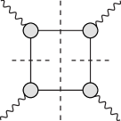
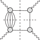
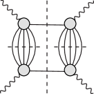
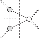
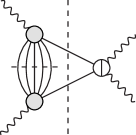
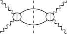
Figure 3: Classes of unitarity diagrams in HLbL scattering. The grey blobs denote (transition) form factors and the blobs with vertical line a polynomial contribution in the crossed channel.

The use and interpretation of (3.4) requires some discussion. In particular, we return to the separation of the FsQED term from the rest which we introduced in Sect. 2.2. To implement this separation correctly and avoid double counting, we must specify what we mean by the partial waves of $\gamma^{*}\gamma^{*}\to\pi^{+}\pi^{-}$ which appear in (3.4) via the $I_{i,(s,u)}$ (see App. G and (3.2)). We decompose the charged-pion partial waves into Born terms $N_{J,\lambda_{1}\lambda_{2}}$ (see App. A) and a remainder $\hat{h}_{J,\lambda_{1}\lambda_{2}}$ to obtain the decomposition ($i=\lambda_{1}\lambda_{2}$, $j=\lambda_{3}\lambda_{4}$)

$$h_{J,i}\big{(}s;q_{1}^{2},q_{2}^{2}\big{)}h_{J,j}^{*}\big{(}s;q_{3}^{2},0\big{)} =N_{J,i}\big{(}s;q_{1}^{2},q_{2}^{2}\big{)}N_{J,j}\big{(}s;q_{3}^{2},0\big{)}+N_{J,i}\big{(}s;q_{1}^{2},q_{2}^{2}\big{)}\hat{h}_{J,j}^{*}\big{(}s;q_{3}^{2},0\big{)}$$

$$+\hat{h}_{J,i}\big{(}s;q_{1}^{2},q_{2}^{2}\big{)}N_{J,j}\big{(}s;q_{3}^{2},0\big{)}+\hat{h}_{J,i}\big{(}s;q_{1}^{2},q_{2}^{2}\big{)}\hat{h}_{J,j}^{*}\big{(}s;q_{3}^{2},0\big{)}.$$ (3.19)

The first term has to be removed from all the $I_{i,(s,u)}$ entering (3.4) since it is accounted for by the FsQED charged pion loop, see (3.2). The second and third term correspond to a triangle-type contribution (fourth diagram in Fig. 3), and the last term to a bulb topology (last diagram in Fig. 3). Physically, the amplitudes $\hat{h}_{J,\lambda_{1}\lambda_{2}}$ include for instance $\pi\pi$ rescattering effects, and thus allow for a model-independent treatment of degrees of freedom corresponding to resonances coupling to the $\pi\pi$ channel, such as the $\sigma$-resonance.

We now discuss in more detail the precise meaning of our initial statement that in our dispersive approach we neglected multi-pion intermediate states. Consider the different classes of unitarity diagrams that involve $\pi\pi$ intermediate states in the $s$-channel, as shown in Fig. 3. Although, by definition, all these diagrams are $\pi\pi$ reducible in the $s$-channel, they differ in the analytic structure in the crossed channel: sub-diagrams feature a pion pole, multi-pion exchange, or polynomial contributions. Our dispersive representation of the HLbL amplitude was derived in a partial-wave picture and therefore cannot, by construction, have any crossed-channel cut. Box diagrams with multi-pion exchange involve crossed-channel multi-pion cuts, representing intermediate states with more than two pions. These unitarity diagrams are not neglected completely, but only included in a partial-wave approximation. In this framework, the second diagram in Fig. 3 is partially covered by the second and third term in (3.4), because the partial-wave projection of the left-hand side of the diagram (which contains the multi-pion exchange) is contained in $\hat{h}_{J,j}$. Analogously the third and fifth diagram belong to the last term therein. Indeed, if the first term in (3.4) is kept, the contribution from the dispersive integrals in (3.4) exactly corresponds to the first term of the partial-wave expansion of the charged-pion loop calculated within sQED multiplied by the appropriate power of the pion vector form factor.

The subtleties concerning Born terms are absent for neutral pions. However, since we have assumed distinguishable particles in the derivation of the unitarity relation, their contribution has to be accompanied by a symmetry factor of $1/2$, see (3.2), so that the explicit form of the $\gamma^{*}\gamma^{*}\to\pi\pi$ amplitudes occurring in the imaginary part reads

$$\mathcal{S}\Big{[}h_{J,i}^{\text{c}}\big{(}s;q_{1}^{2},q_{2}^{2}\big{)}\Big{(}h_{J,j}^{\text{c}}\big{(}s;q_{3}^{2},0\big{)}\Big{)}^{*}\Big{]}+\mathcal{S}\Big{[}h_{J,i}^{\text{n}}\big{(}s;q_{1}^{2},q_{2}^{2}\big{)}\Big{(}h_{J,j}^{\text{n}}\big{(}s;q_{3}^{2},0\big{)}\Big{)}^{*}\Big{]}$$ (3.20)

$$=h_{J,i}^{\text{c}}\big{(}s;q_{1}^{2},q_{2}^{2}\big{)}\Big{(}h_{J,j}^{\text{c}}\big{(}s;q_{3}^{2},0\big{)}\Big{)}^{*}+\frac{1}{2}h_{J,i}^{\text{n}}\big{(}s;q_{1}^{2},q_{2}^{2}\big{)}\Big{(}h_{J,j}^{\text{n}}\big{(}s;q_{3}^{2},0\big{)}\Big{)}^{*}-N_{J,i}\big{(}s;q_{1}^{2},q_{2}^{2}\big{)}N_{J,j}\big{(}s;q_{3}^{2},0\big{)},$$

adding the contributions from charged and neutral pions and subtracting the FsQED part. Alternatively, (3.20) may be expressed in the isospin basis. Changing basis towards isospin $0$ and $2$ according to [37]

$$\begin{pmatrix}h_{J,i}^{\text{c}}\\ h_{J,i}^{\text{n}}\end{pmatrix}=\begin{pmatrix}\frac{1}{\sqrt{3}}&\frac{1}{\sqrt{6}}\\ \frac{1}{\sqrt{3}}&-\sqrt{\frac{2}{3}}\end{pmatrix}\begin{pmatrix}h_{J,i}^{0}\\ h_{J,i}^{2}\end{pmatrix},$$ (3.21)

we find

$$\mathcal{S}\Big{[}h_{J,i}^{\text{c}}\big{(}s;q_{1}^{2},q_{2}^{2}\big{)}\Big{(}h_{J,j}^{\text{c}}\big{(}s;q_{3}^{2},0\big{)}\Big{)}^{*}\Big{]}+\mathcal{S}\Big{[}h_{J,i}^{\text{n}}\big{(}s;q_{1}^{2},q_{2}^{2}\big{)}\Big{(}h_{J,j}^{\text{n}}\big{(}s;q_{3}^{2},0\big{)}\Big{)}^{*}\Big{]}$$ (3.22)

$$=\frac{1}{2}h_{J,i}^{0}\big{(}s;q_{1}^{2},q_{2}^{2}\big{)}\Big{(}h_{J,j}^{0}\big{(}s;q_{3}^{2},0\big{)}\Big{)}^{*}+\frac{1}{2}h_{J,i}^{2}\big{(}s;q_{1}^{2},q_{2}^{2}\big{)}\Big{(}h_{J,j}^{2}\big{(}s;q_{3}^{2},0\big{)}\Big{)}^{*}-N_{J,i}\big{(}s;q_{1}^{2},q_{2}^{2}\big{)}N_{J,j}\big{(}s;q_{3}^{2},0\big{)}.$$

As long as the virtualities remain below the two-pion threshold, Watson’s theorem [43] implies that the phase of $h_{J,i}^{I}\big{(}s;q_{1}^{2},q_{2}^{2}\big{)}$ is equal to $\delta_{J}^{I}(s)$, the phase shift of the corresponding $\pi\pi$ partial wave. Since the Born terms $N_{J,i}\big{(}s;q_{1}^{2},q_{2}^{2}\big{)}$ are real, this proves that indeed the final result for the imaginary part is a real quantity.

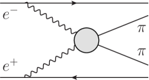
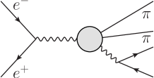
Figure 4: $\gamma^{*}\gamma^{*}\to\pi\pi$ physics in space-like (left) and time-like (right) kinematics.

Experimentally, $\gamma^{*}\gamma^{*}\to\pi\pi$ partial waves are accessible in the process $e^{+}e^{-}\to e^{+}e^{-}\pi\pi$, either in space-like or time-like configuration, see Fig. 4. Using similar manipulations of the loop integrals as in the case of the pion pole [15, 1], only negative virtualities are required for HLbL scattering. However, within the dispersive approach information from all kinematic regions is highly welcome to provide additional experimental constraints and potentially improve the accuracy, as dispersion theory is the ideal framework to reliably perform the required analytic continuation. In this particular case, the construction of dispersion relations for the doubly-virtual process $\gamma^{*}\gamma^{*}\to\pi\pi$ in time-like kinematics is complicated by the occurrence of anomalous thresholds [26, 27]. For a description of how to account for those effects within our framework see [28].

In summary, we obtain a decomposition of the full HLbL contribution into

$$a_{\mu}^{\text{HLbL}}=a_{\mu}^{\pi^{0}\text{-pole}}+a_{\mu}^{\text{FsQED}}+a_{\mu}^{\pi\pi},$$ (3.23)

with the pion pole (2.13), the FsQED charged pion loop, and the remaining effects from $\pi\pi$ intermediate states according to (3.4) with imaginary parts as given in (3.20) or (3.22) in particle or isospin basis, respectively. $a_{\mu}^{\pi\pi}$ covers unitarity diagrams both with triangle and bulb topologies. As far as FsQED Born terms are concerned, this is exemplified by the decomposition in (3.4). It should be stressed that both the pion loop and the Born-term contribution to the triangle topologies in $a_{\mu}^{\pi\pi}$ are entirely fixed by the pion vector form factor for the $\pi^{+}\pi^{-}\gamma^{*}$ vertex. Due to the fact that only space-like kinematics are relevant for $a_{\mu}$, the dispersive integrals also for triangle topologies are free of anomalous thresholds. But even if they were not, the present formalism would still be useful: one would merely have to extend the framework along the lines sketched in [28].

4 Conclusions and outlook

The main result of this paper is presented in (3.23) and (3.4): a master formula that gives the contribution from $\pi\pi$ intermediate states in HLbL scattering to the anomalous magnetic moment of the muon, expressed in terms of helicity partial waves for $\gamma^{*}\gamma^{*}\to\pi\pi$. Within the general framework of dispersion theory, $\pi\pi$ intermediate states constitute the second most important contribution after pseudoscalar pole terms, also included in (3.23). This result is important progress towards a model-independent, data-driven analysis of HLbL scattering. A first numerical evaluation of these contributions as they appear in (3.23) and (3.4) as well as a generalization to a complete treatment of $D$-waves is in progress [32].

Although in principle the required helicity partial waves for $\gamma^{*}\gamma^{*}\to\pi\pi$ can be measured, a dispersive treatment of $\gamma^{*}\gamma^{*}\to\pi\pi$ in the framework of Roy–Steiner equations allows for a combined analysis of all experimental constraints available for the relevant pion–photon interactions [37, 32], in particular from kinematic regions different from those directly relevant for HLbL scattering. While heavier two-particle, scalar intermediate states (such as $K\bar{K}$) are amenable to the same treatment, it is more challenging to account for multi-pion contributions at the same level of rigor that we have adhered to here. To estimate the impact of multi-pion intermediate states, possible ansätze would be to try to generalize the calculation of the FsQED pion loop to include resonances or to approximate missing physical degrees of freedom in terms of resonance poles along the lines of [46].

The final goal of the approach laid out here is a calculation of HLbL scattering consistent with the general principles of analyticity, unitarity, crossing symmetry, and gauge invariance and backed by data as closely as possible. To this end, also the pseudoscalar transition form factors should be subject to a similar analysis, see [47, 48, 49, 50] for first steps in this direction. Ultimately, this approach should allow for a more reliable estimate of uncertainties in the HLbL contribution to the anomalous magnetic moment of the muon.

Acknowledgements

We would like to thank Andreas Nyffeler for helpful discussions, and Bastian Kubis, Heiri Leutwyler, and Andreas Nyffeler for comments on the manuscript. Financial support by the Swiss National Science Foundation is gratefully acknowledged. The AEC is supported by the “Innovations- und Kooperationsprojekt C-13” of the “Schweizerische Universitätskonferenz SUK/CRUS.”

Appendix A FsQED Born terms and contribution to $\boldsymbol{a_{\mu}}$

In our conventions, the $S$- and $D$-wave projections of the Born terms for $\gamma^{*}\gamma^{*}\to\pi\pi$ read [32]

$$N_{J,++}\big{(}t;q_{1}^{2},q_{2}^{2}\big{)} =\Bigg{\{}\frac{2}{p_{t}q_{t}}Q_{J}(x_{t})\bigg{(}M_{\pi}^{2}+\frac{tq_{1}^{2}q_{2}^{2}}{\lambda_{12}^{t}}\bigg{)}+2\delta_{J0}\frac{\big{(}q_{1}^{2}-q_{2}^{2}\big{)}^{2}-t\big{(}q_{1}^{2}+q_{2}^{2}\big{)}}{\lambda_{12}^{t}}\Bigg{\}}F_{\pi}^{V}\big{(}q_{1}^{2}\big{)}F_{\pi}^{V}\big{(}q_{2}^{2}\big{)},$$

$$N_{2,+-}\big{(}t;q_{1}^{2},q_{2}^{2}\big{)} =\Bigg{\{}-\frac{2}{p_{t}q_{t}}\bigg{(}d_{20}^{2}(x_{t})Q_{0}(x_{t})+\frac{\sqrt{6}}{4}x_{t}\bigg{)}\bigg{(}M_{\pi}^{2}+\frac{tq_{1}^{2}q_{2}^{2}}{\lambda_{12}^{t}}\bigg{)}+\frac{2}{\sqrt{6}}\frac{t\big{(}t-q_{1}^{2}-q_{2}^{2}\big{)}}{\lambda_{12}^{t}}\Bigg{\}}$$

$$\qquad\times F_{\pi}^{V}\big{(}q_{1}^{2}\big{)}F_{\pi}^{V}\big{(}q_{2}^{2}\big{)},$$

$$N_{2,+0}\big{(}t;q_{1}^{2},q_{2}^{2}\big{)} =-\frac{t+q_{1}^{2}-q_{2}^{2}}{t-q_{1}^{2}-q_{2}^{2}}\frac{q_{2}^{2}}{\xi_{2}}\sqrt{\frac{3}{t}}\frac{2p_{t}}{q_{t}}\bigg{\{}x_{t}^{2}\big{(}1-x_{t}^{2}\big{)}Q_{0}(x_{t})+x_{t}\bigg{(}x_{t}^{2}-\frac{2}{3}\bigg{)}\bigg{\}}F_{\pi}^{V}\big{(}q_{1}^{2}\big{)}F_{\pi}^{V}\big{(}q_{2}^{2}\big{)},$$

$$N_{2,0+}\big{(}t;q_{1}^{2},q_{2}^{2}\big{)} =-\frac{t-q_{1}^{2}+q_{2}^{2}}{t-q_{1}^{2}-q_{2}^{2}}\frac{q_{1}^{2}}{\xi_{1}}\sqrt{\frac{3}{t}}\frac{2p_{t}}{q_{t}}\bigg{\{}x_{t}^{2}\big{(}1-x_{t}^{2}\big{)}Q_{0}(x_{t})+x_{t}\bigg{(}x_{t}^{2}-\frac{2}{3}\bigg{)}\bigg{\}}F_{\pi}^{V}\big{(}q_{1}^{2}\big{)}F_{\pi}^{V}\big{(}q_{2}^{2}\big{)},$$

$$N_{J,00}\big{(}t;q_{1}^{2},q_{2}^{2}\big{)} =-\frac{q_{1}^{2}q_{2}^{2}}{\xi_{1}\xi_{2}\lambda_{12}^{t}}\bigg{\{}\Big{(}t^{2}-\big{(}q_{1}^{2}-q_{2}^{2}\big{)}^{2}\Big{)}\frac{1}{p_{t}q_{t}}Q_{J}(x_{t})-8t\delta_{J0}\bigg{\}}F_{\pi}^{V}\big{(}q_{1}^{2}\big{)}F_{\pi}^{V}\big{(}q_{2}^{2}\big{)},$$ (A.1)

with

$$x_{t}=\frac{t-q_{1}^{2}-q_{2}^{2}}{4p_{t}q_{t}},$$ (A.2)

and the lowest Legendre functions of the second kind

$$Q_{0}(z)=\frac{1}{2}\int\limits_{-1}^{1}\frac{\text{d}x}{z-x},\qquad Q_{0}(z\pm i\epsilon)=\frac{1}{2}\log\bigg{|}\frac{1+z}{1-z}\bigg{|}\mp i\frac{\pi}{2}\theta\big{(}1-z^{2}\big{)},\qquad Q_{2}(z)=P_{2}(z)Q_{0}(z)-\frac{3}{2}z.$$ (A.3)

$F_{\pi}^{V}(q^{2})$ denotes the pion vector form factor and the kinematic quantities are defined as in Sect. 2.4.

However, for the reasons discussed in Sects. 2.2 and 3.4 the FsQED contribution to $a_{\mu}$ cannot be analyzed within a partial-wave framework, but rather based on Feynman integrals. We find the representation

$$a_{\mu}^{\text{FsQED}}=\frac{2e^{6}}{3\pi^{2}}\int\frac{\text{d}^{4}q_{1}}{(2\pi)^{4}}\int\frac{\text{d}^{4}q_{2}}{(2\pi)^{4}}\frac{F_{\pi}^{V}\big{(}q_{1}^{2}\big{)}F_{\pi}^{V}\big{(}q_{2}^{2}\big{)}F_{\pi}^{V}(s)\big{(}I_{s}+2I_{u}+J_{1}+J_{2}\big{)}}{q_{1}^{2}q_{2}^{2}s\big{(}(p+q_{1})^{2}-m^{2}\big{)}\big{(}(p-q_{2})^{2}-m^{2}\big{)}},$$ (A.4)

where

$$I_{s} =\Big{\{}m^{2}s-2p\cdot q_{1}\big{(}p\cdot q_{1}+p\cdot q_{2}-q_{1}\cdot q_{2}-q_{2}^{2}\big{)}\Big{\}}\int\limits_{0}^{1}\text{d}x\frac{x(1-x)}{M_{\pi}^{2}-x(1-x)s},$$ (A.5)

$$I_{u} =\Big{\{}q_{1}^{2}\big{(}m^{2}+p\cdot q_{2}\big{)}-p\cdot q_{1}\big{(}p\cdot q_{1}+q_{1}\cdot q_{2}\big{)}\Big{\}}\int\limits_{0}^{1}\text{d}x\frac{x(1-x)}{M_{\pi}^{2}-x(1-x)q_{1}^{2}},$$

$$J_{1} =\int\limits_{0}^{1}\text{d}x\int\limits_{0}^{1-x}\text{d}y\,\Delta^{-1}(x,y)\Bigg{\{}2(16xy-6x-6y+3)p\cdot q_{1}\,p\cdot q_{2}-4x(8x-5)(p\cdot q_{1})^{2}$$

$$+2p\cdot q_{1}\Big{[}2x(5x+2y-3)q_{1}\cdot q_{2}-\big{(}8xy+2y^{2}-6x-6y+3\big{)}q_{2}^{2}\Big{]}-8m^{2}x(y\,q_{1}\cdot q_{2}+(1-x)q_{1}^{2}\big{)}\Bigg{\}},$$

$$J_{2} =\int\limits_{0}^{1}\text{d}x\int\limits_{0}^{1-x}\text{d}y\,\Delta^{-2}(x,y)\Bigg{\{}\frac{m^{2}}{2}xy(1-x-y)\lambda_{12}$$

$$+2(p\cdot q_{1})^{2}\Big{[}x(x+2y-1)q_{1}\cdot q_{2}+y\big{(}2x(x+y-1)+1-y\big{)}q_{2}^{2}\Big{]}$$

$$-p\cdot q_{1}\,p\cdot q_{2}\Big{[}\big{(}x^{2}(4y-1)+x(1-2y)^{2}+y(1-y)\big{)}q_{1}\cdot q_{2}+x(x+2y-1)q_{1}^{2}+y(2x+y-1)q_{2}^{2}\Big{]}$$

$$+p\cdot q_{1}\bigg{[}y\Big{[}(1-2y)^{2}(2x+y-1)q_{2}^{2}-(2x-1)\big{(}4x^{2}+6x(y-1)+1-y\big{)}q_{1}^{2}\Big{]}q_{2}^{2}$$

$$+x\Big{[}8(x-1)xy\,q_{1}\cdot q_{2}+(1-2x)^{2}(x+2y-1)q_{1}^{2}-\big{(}4(3x-2)y^{2}+(8y-1)(1-x)\big{)}q_{2}^{2}\Big{]}q_{1}\cdot q_{2}\bigg{]}\Bigg{\}},$$

and

$$\Delta(x,y)=M_{\pi}^{2}-xys-x(1-x-y)q_{1}^{2}-y(1-x-y)q_{2}^{2}.$$ (A.6)

Appendix B $\boldsymbol{1}$-loop ChPT for $\boldsymbol{\gamma^{*}\gamma^{*}\to\pi\pi}$

At $1$-loop order the only non-vanishing partial-wave amplitudes are (for the on-shell case see [51, 52])

$$h_{0,++}\big{(}t;q_{1}^{2},q_{2}^{2}\big{)} =\frac{\bar{l}_{6}-\bar{l}_{5}}{48\pi^{2}F_{\pi}^{2}}\big{(}t-q_{1}^{2}-q_{2}^{2}\big{)}\begin{Bmatrix}1\\ 0\end{Bmatrix}-\frac{1}{8\pi^{2}F_{\pi}^{2}}\begin{Bmatrix}t/2\\ t-M_{\pi}^{2}\end{Bmatrix}\Bigg{\{}1+2\bigg{(}M_{\pi}^{2}+\frac{tq_{1}^{2}q_{2}^{2}}{\lambda_{12}^{t}}\bigg{)}C_{0}\big{(}t,q_{1}^{2},q_{2}^{2}\big{)}$$

$$+\frac{t\big{(}q_{1}^{2}+q_{2}^{2}\big{)}-\big{(}q_{1}^{2}-q_{2}^{2}\big{)}^{2}}{\lambda_{12}^{t}}\bar{J}(t)-\frac{q_{1}^{2}\big{(}t+q_{2}^{2}-q_{1}^{2}\big{)}}{\lambda_{12}^{t}}\bar{J}\big{(}q_{1}^{2}\big{)}-\frac{q_{2}^{2}\big{(}t+q_{1}^{2}-q_{2}^{2}\big{)}}{\lambda_{12}^{t}}\bar{J}\big{(}q_{2}^{2}\big{)}\Bigg{\}},$$

$$h_{0,00}\big{(}t;q_{1}^{2},q_{2}^{2}\big{)} =\frac{q_{1}^{2}q_{2}^{2}}{\xi_{1}\xi_{2}}\Bigg{[}\frac{\bar{l}_{6}-\bar{l}_{5}}{24\pi^{2}F_{\pi}^{2}}\begin{Bmatrix}1\\ 0\end{Bmatrix}+\frac{1}{8\pi^{2}F_{\pi}^{2}\lambda_{12}^{t}}\begin{Bmatrix}t/2\\ t-M_{\pi}^{2}\end{Bmatrix}\bigg{\{}\Big{(}t^{2}-\big{(}q_{1}^{2}-q_{2}^{2}\big{)}^{2}\Big{)}C_{0}\big{(}t,q_{1}^{2},q_{2}^{2}\big{)}$$

$$+4t\bar{J}(t)-2\big{(}t+q_{1}^{2}-q_{2}^{2}\big{)}\bar{J}\big{(}q_{1}^{2}\big{)}-2\big{(}t-q_{1}^{2}+q_{2}^{2}\big{)}\bar{J}\big{(}q_{2}^{2}\big{)}\bigg{\}}\Bigg{]},$$ (B.1)

where the upper/lower result refers to charged/neutral pions and the loop functions are defined as

$$C_{0}\big{(}t,q_{1}^{2},q_{2}^{2}\big{)} =-\int\limits_{0}^{1}\text{d}x\int\limits_{0}^{1-x}\text{d}y\frac{1}{M_{\pi}^{2}-txy-q_{1}^{2}x(1-x-y)-q_{2}^{2}y(1-x-y)},$$

$$\bar{J}(t) =-\int\limits_{0}^{1}\text{d}x\log\bigg{[}1-x(1-x)\frac{t}{M_{\pi}^{2}}\bigg{]},$$ (B.2)

with imaginary parts

$$\text{Im}_{t}\,\bar{J}(t)=\pi\sigma_{t}\theta\big{(}t-4M_{\pi}^{2}\big{)},\qquad\text{Im}_{t}\,C_{0}\big{(}t,q_{1}^{2},q_{2}^{2}\big{)}=-\frac{\pi\theta\big{(}t-4M_{\pi}^{2}\big{)}}{\sqrt{\lambda_{12}^{t}}}\log\frac{t-q_{1}^{2}-q_{2}^{2}+\sigma_{t}\sqrt{\lambda_{12}^{t}}}{t-q_{1}^{2}-q_{2}^{2}-\sigma_{t}\sqrt{\lambda_{12}^{t}}}.$$ (B.3)

In the limit $q_{i}^{2}\to 0$, (B) reproduces the leading term of the chiral expansion of the pion polarizabilities

$$h_{0,++}(t;0,0)=\frac{M_{\pi}}{2\alpha}\big{(}\alpha_{1}-\beta_{1}\big{)}t+\mathcal{O}\big{(}t^{2}\big{)},\qquad\frac{M_{\pi}}{2\alpha}\big{(}\alpha_{1}-\beta_{1}\big{)}=\frac{1}{96\pi^{2}F_{\pi}^{2}}\begin{Bmatrix}2(\bar{l}_{6}-\bar{l}_{5})\\ -1\end{Bmatrix}.$$ (B.4)

In practice, subtractions have to be introduced into the Roy–Steiner equations for $\gamma^{*}\gamma^{*}\to\pi\pi$ sketched in Sect. 2.4 in order to suppress the high-energy tail of the integrals. The ChPT result (B) as well as experimental information on pion polarizabilities provide valuable constraints for this subtraction term. Moreover, the $1$-loop chiral amplitudes themselves can be used to illustrate the $S$-wave part of the Roy–Steiner system (2.4) and (2.31). Inserting (B) into these equations, one finds the relations

$$\frac{1}{\pi}\int\limits_{4M_{\pi}^{2}}^{\infty}\text{d}t^{\prime}\Bigg{\{}\bigg{(}\frac{1}{t^{\prime}-t}-\frac{t^{\prime}-q_{1}^{2}-q_{2}^{2}}{\lambda_{12}^{t^{\prime}}}\bigg{)}\text{Im}_{t}\,h_{1}\big{(}t^{\prime};q_{1}^{2},q_{2}^{2}\big{)}+\frac{2q_{1}^{2}q_{2}^{2}}{\lambda_{12}^{t^{\prime}}}\text{Im}_{t}\,h_{2}\big{(}t^{\prime};q_{1}^{2},q_{2}^{2}\big{)}\Bigg{\}}$$ (B.5)

$$=1+2\bigg{(}M_{\pi}^{2}+\frac{tq_{1}^{2}q_{2}^{2}}{\lambda_{12}^{t}}\bigg{)}C_{0}\big{(}t,q_{1}^{2},q_{2}^{2}\big{)}+\frac{t\big{(}q_{1}^{2}+q_{2}^{2}\big{)}-\big{(}q_{1}^{2}-q_{2}^{2}\big{)}^{2}}{\lambda_{12}^{t}}\bar{J}(t)$$

$$\quad-\frac{q_{1}^{2}\big{(}t+q_{2}^{2}-q_{1}^{2}\big{)}}{\lambda_{12}^{t}}\bar{J}\big{(}q_{1}^{2}\big{)}-\frac{q_{2}^{2}\big{(}t+q_{1}^{2}-q_{2}^{2}\big{)}}{\lambda_{12}^{t}}\bar{J}\big{(}q_{2}^{2}\big{)},$$

$$\frac{1}{\pi}\int\limits_{4M_{\pi}^{2}}^{\infty}\text{d}t^{\prime}\Bigg{\{}\bigg{(}\frac{1}{t^{\prime}-t}-\frac{t^{\prime}-q_{1}^{2}-q_{2}^{2}}{\lambda_{12}^{t^{\prime}}}\bigg{)}\text{Im}_{t}\,h_{2}\big{(}t^{\prime};q_{1}^{2},q_{2}^{2}\big{)}+\frac{2}{\lambda_{12}^{t^{\prime}}}\text{Im}_{t}\,h_{1}\big{(}t^{\prime};q_{1}^{2},q_{2}^{2}\big{)}\Bigg{\}}$$

$$=-\frac{1}{\lambda_{12}^{t}}\bigg{\{}\Big{(}t^{2}-\big{(}q_{1}^{2}-q_{2}^{2}\big{)}^{2}\Big{)}C_{0}\big{(}t,q_{1}^{2},q_{2}^{2}\big{)}+4t\bar{J}(t)-2\big{(}t+q_{1}^{2}-q_{2}^{2}\big{)}\bar{J}\big{(}q_{1}^{2}\big{)}-2\big{(}t-q_{1}^{2}+q_{2}^{2}\big{)}\bar{J}\big{(}q_{2}^{2}\big{)}\bigg{\}},$$

where $h_{1}$ and $h_{2}$ with imaginary parts

$$\text{Im}_{t}\,h_{1}\big{(}t;q_{1}^{2},q_{2}^{2}\big{)} =2\bigg{(}M_{\pi}^{2}+\frac{tq_{1}^{2}q_{2}^{2}}{\lambda_{12}^{t}}\bigg{)}\text{Im}_{t}\,C_{0}\big{(}t,q_{1}^{2},q_{2}^{2}\big{)}+\frac{t\big{(}q_{1}^{2}+q_{2}^{2}\big{)}-\big{(}q_{1}^{2}-q_{2}^{2}\big{)}^{2}}{\lambda_{12}^{t}}\text{Im}_{t}\,\bar{J}(t),$$

$$\text{Im}_{t}\,h_{2}\big{(}t;q_{1}^{2},q_{2}^{2}\big{)} =-\frac{1}{\lambda_{12}^{t}}\Big{[}\Big{(}t^{2}-\big{(}q_{1}^{2}-q_{2}^{2}\big{)}^{2}\Big{)}\text{Im}_{t}\,C_{0}\big{(}t,q_{1}^{2},q_{2}^{2}\big{)}+4t\text{Im}_{t}\,\bar{J}(t)\Big{]},$$ (B.6)

correspond to $h_{0,++}$ and $h_{0,00}$, respectively. We checked numerically that the relations (B.5) hold. In particular, we find that in general the contribution from the non-diagonal kernels is non-negligible.

Appendix C Lorentz structures for the HLbL tensor

The Lorentz structures that appear in the unitarity relation (3.1) are

$$A_{1,s}^{\mu\nu\lambda\sigma} =\frac{8}{\big{(}s-q_{3}^{2}\big{)}\lambda_{12}}\Big{(}k^{\lambda}q_{3}^{\sigma}-k\cdot q_{3}\,g^{\lambda\sigma}\Big{)}\bigg{(}q^{\mu\nu}_{12}+\frac{\lambda_{12}}{4}g^{\mu\nu}\bigg{)},$$

$$A_{2,s}^{\mu\nu\lambda\sigma} =\frac{8}{\big{(}s-q_{3}^{2}\big{)}\lambda_{12}}\Big{(}k^{\lambda}q_{3}^{\sigma}-k\cdot q_{3}\,g^{\lambda\sigma}\Big{)}\Big{(}q_{1}\cdot q_{2}\,q_{1}^{\mu}-q_{1}^{2}\,q_{2}^{\mu}\Big{)}\Big{(}q_{2}^{2}\,q_{1}^{\nu}-q_{1}\cdot q_{2}\,q_{2}^{\nu}\Big{)},$$

$$A_{3,s}^{\mu\nu\lambda\sigma} =-\frac{8}{5\big{(}s-q_{3}^{2}\big{)}\lambda_{12}}\bigg{\{}\big{(}1-z_{s}^{2}\big{)}\Big{(}k^{\lambda}q_{3}^{\sigma}-k\cdot q_{3}\,g^{\lambda\sigma}\Big{)}+\frac{4s\,q_{tu}^{\lambda}q_{tu}^{\sigma}}{\big{(}s-q_{3}^{2}\big{)}\lambda_{12}}\bigg{\}}\bigg{(}q^{\mu\nu}_{12}+\frac{\lambda_{12}}{4}g^{\mu\nu}\bigg{)},$$

$$A_{4,s}^{\mu\nu\lambda\sigma} =\frac{32\bar{z}_{s}\,q_{tu}^{\sigma}}{5\big{(}s-q_{3}^{2}\big{)}^{2}\lambda_{12}}\Big{(}k\cdot q_{3}\,q_{3}^{\lambda}-q_{3}^{2}\,k^{\lambda}\Big{)}\bigg{(}q^{\mu\nu}_{12}+\frac{\lambda_{12}}{4}g^{\mu\nu}\bigg{)},$$

$$A_{5,s}^{\mu\nu\lambda\sigma} =-\frac{4}{5\big{(}s-q_{3}^{2}\big{)}}\Big{(}k^{\lambda}q_{3}^{\sigma}-k\cdot q_{3}\,g^{\lambda\sigma}\Big{)}\Bigg{\{}\frac{1}{2}\big{(}1-z_{s}^{2}\big{)}g^{\mu\nu}-2\bar{z}_{s}\big{(}q_{1}^{\mu}q_{1}^{\nu}-q_{2}^{\mu}q_{2}^{\nu}\big{)}$$

$$+\big{(}q_{1}^{\mu}+q_{2}^{\mu}\big{)}\big{(}q_{1}^{\nu}+q_{2}^{\nu}\big{)}\frac{1}{s}\Big{(}1+z_{s}^{2}+2\bar{z}_{s}\big{(}q_{1}^{2}-q_{2}^{2}\big{)}\Big{)}+\frac{2\big{(}k^{\mu}k_{s}^{\nu}+k_{s}^{\mu}k^{\nu}\big{)}}{s-q_{3}^{2}}+\frac{2}{\lambda_{12}}\big{(}1+z_{s}^{2}\big{)}q^{\mu\nu}_{12}\Bigg{\}},$$

$$A_{6,s}^{\mu\nu\lambda\sigma} =\frac{16}{15\big{(}s-q_{3}^{2}\big{)}^{2}\lambda_{12}}\Bigg{\{}-\frac{\big{(}s-q_{3}^{2}\big{)}^{2}\lambda_{12}}{4}\big{(}g^{\mu\lambda}g^{\nu\sigma}+g^{\mu\sigma}g^{\nu\lambda}\big{)}$$

$$+\frac{s-q_{3}^{2}}{2}\Bigg{[}g^{\mu\nu}\bigg{[}\frac{\lambda_{12}}{2}\big{(}z_{s}^{2}-3\big{)}\Big{(}k^{\lambda}q_{3}^{\sigma}-k\cdot q_{3}\,g^{\lambda\sigma}\Big{)}-\frac{2s}{s-q_{3}^{2}}\,q_{tu}^{\lambda}q_{tu}^{\sigma}\bigg{]}$$

$$+g^{\mu\lambda}\bigg{[}\lambda_{12}\Big{(}k^{\nu}q_{3}^{\sigma}-k\cdot q_{3}\,g^{\nu\sigma}\Big{)}-q_{tu}^{\sigma}\Big{(}\big{(}s-q_{1}^{2}+q_{2}^{2}\big{)}q_{1}^{\nu}-\big{(}s+q_{1}^{2}-q_{2}^{2}\big{)}q_{2}^{\nu}\Big{)}\bigg{]}$$

$$+g^{\nu\lambda}\bigg{[}\lambda_{12}\Big{(}k^{\mu}q_{3}^{\sigma}-k\cdot q_{3}\,g^{\mu\sigma}\Big{)}-q_{tu}^{\sigma}\Big{(}\big{(}s-q_{1}^{2}+q_{2}^{2}\big{)}q_{1}^{\mu}-\big{(}s+q_{1}^{2}-q_{2}^{2}\big{)}q_{2}^{\mu}\Big{)}\bigg{]}$$

$$+g^{\mu\sigma}\bigg{[}\lambda_{12}\Big{(}q_{3}^{\nu}k^{\lambda}-k\cdot q_{3}\,g^{\nu\lambda}\Big{)}+q_{tu}^{\lambda}\Big{(}\big{(}q_{1}^{2}-q_{2}^{2}\big{)}\big{(}q_{1}^{\nu}+q_{2}^{\nu}\big{)}-s\big{(}q_{1}^{\nu}-q_{2}^{\nu}\big{)}\Big{)}-\frac{2\lambda_{12}\,k^{\nu}}{s-q_{3}^{2}}\Big{(}k\cdot q_{3}\,q_{3}^{\lambda}-q_{3}^{2}\,k^{\lambda}\Big{)}\bigg{]}$$

$$+g^{\nu\sigma}\bigg{[}\lambda_{12}\Big{(}q_{3}^{\mu}k^{\lambda}-k\cdot q_{3}\,g^{\mu\lambda}\Big{)}+q_{tu}^{\lambda}\Big{(}\big{(}q_{1}^{2}-q_{2}^{2}\big{)}\big{(}q_{1}^{\mu}+q_{2}^{\mu}\big{)}-s\big{(}q_{1}^{\mu}-q_{2}^{\mu}\big{)}\Big{)}-\frac{2\lambda_{12}\,k^{\mu}}{s-q_{3}^{2}}\Big{(}k\cdot q_{3}\,q_{3}^{\lambda}-q_{3}^{2}\,k^{\lambda}\Big{)}\bigg{]}\Bigg{]}$$

$$-\lambda_{12}\Big{(}k^{\lambda}q_{3}^{\sigma}-k\cdot q_{3}\,g^{\lambda\sigma}\Big{)}\Bigg{[}k^{\mu}k_{s}^{\nu}+k_{s}^{\mu}k^{\nu}+\frac{s-q_{3}^{2}}{2s}\bigg{[}\Big{(}1+z_{s}^{2}+2\bar{z}_{s}\big{(}q_{1}^{2}-q_{2}^{2}\big{)}\Big{)}\big{(}q_{1}^{\mu}+q_{2}^{\mu}\big{)}\big{(}q_{1}^{\nu}+q_{2}^{\nu}\big{)}$$

$$\qquad-2s\bar{z}_{s}\big{(}q_{1}^{\mu}q_{1}^{\nu}-q_{2}^{\mu}q_{2}^{\nu}\big{)}+\frac{2s}{\lambda_{12}}\big{(}z_{s}^{2}+3\big{)}q_{12}^{\mu\nu}\bigg{]}\Bigg{]}$$

$$+2q_{tu}^{\sigma}\bigg{[}q_{tu}^{\lambda}\Big{(}\big{(}q_{1}^{\mu}+q_{2}^{\mu}\big{)}\big{(}q_{1}^{\nu}+q_{2}^{\nu}\big{)}+\frac{2s}{\lambda_{12}}q_{12}^{\mu\nu}\Big{)}-k^{\lambda}\Big{(}\big{(}q_{1}^{2}-q_{2}^{2}\big{)}\big{(}q_{1}^{\mu}+q_{2}^{\mu}\big{)}\big{(}q_{1}^{\nu}+q_{2}^{\nu}\big{)}-s\big{(}q_{1}^{\mu}q_{1}^{\nu}-q_{2}^{\mu}q_{2}^{\nu}\big{)}\Big{)}\bigg{]}$$

$$+\bigg{[}2\big{(}q_{1}^{\lambda}+q_{2}^{\lambda}\big{)}q_{tu}^{\sigma}-\big{(}s-q_{3}^{2}\big{)}\big{(}q_{1}^{\lambda}q_{2}^{\sigma}-q_{2}^{\lambda}q_{1}^{\sigma}\big{)}+2\lambda_{12}\bar{z}_{s}k^{\lambda}q_{3}^{\sigma}\bigg{]}$$

$$\qquad\times\bigg{[}\big{(}s-q_{1}^{2}+q_{2}^{2}\big{)}\big{(}q_{1}^{\mu}k^{\nu}+k^{\mu}q_{1}^{\nu}\big{)}-\big{(}s+q_{1}^{2}-q_{2}^{2}\big{)}\big{(}q_{2}^{\mu}k^{\nu}+k^{\mu}q_{2}^{\nu}\big{)}\bigg{]}$$

$$+2k^{\lambda}\bigg{[}s\Big{(}k^{\nu}\big{(}q_{1}^{\mu}+q_{2}^{\mu}\big{)}+k^{\mu}\big{(}q_{1}^{\nu}+q_{2}^{\nu}\big{)}\Big{)}\big{(}q_{2}^{2}\,q_{1}^{\sigma}+q_{1}^{2}\,q_{2}^{\sigma}\big{)}-s^{2}\Big{(}q_{1}^{\sigma}\big{(}q_{2}^{\mu}k^{\nu}+k^{\mu}q_{2}^{\nu}\big{)}+q_{2}^{\sigma}\big{(}q_{1}^{\mu}k^{\nu}+k^{\mu}q_{1}^{\nu}\big{)}\Big{)}$$

$$\qquad-q_{3}^{\sigma}\Big{(}\big{(}\lambda_{12}+sq_{2}^{2}\big{)}\big{(}q_{1}^{\mu}k^{\nu}+k^{\mu}q_{1}^{\nu}\big{)}+\big{(}\lambda_{12}+sq_{1}^{2}\big{)}\big{(}q_{2}^{\mu}k^{\nu}+k^{\mu}q_{2}^{\nu}\big{)}\Big{)}\bigg{]}$$

$$+\frac{2\lambda_{12}}{s-q_{3}^{2}}k^{\mu}k^{\nu}q_{3}^{\sigma}\Big{(}\big{(}s-q_{3}^{2}\big{)}q_{3}^{\lambda}+\big{(}s+q_{3}^{2}\big{)}k^{\lambda}\Big{)}\Bigg{\}},$$

$$A_{7,s}^{\mu\nu\lambda\sigma} =\frac{16}{15\big{(}s-q_{3}^{2}\big{)}^{2}\lambda_{12}}\Big{(}k\cdot q_{3}\,q_{3}^{\lambda}-q_{3}^{2}\,k^{\lambda}\Big{)}\Bigg{\{}\frac{\lambda_{12}}{s}\Big{(}k^{\mu}q_{3}^{\sigma}-k\cdot q_{3}\,g^{\mu\sigma}\Big{)}\bigg{(}\frac{s\,k^{\nu}}{s-q_{3}^{2}}+k_{s}^{\nu}\bigg{)}$$

$$+\frac{\lambda_{12}}{s}\Big{(}k^{\nu}q_{3}^{\sigma}-k\cdot q_{3}\,g^{\nu\sigma}\Big{)}\bigg{(}\frac{s\,k^{\mu}}{s-q_{3}^{2}}+k_{s}^{\mu}\bigg{)}$$

$$-\frac{2q_{tu}^{\sigma}}{s-q_{3}^{2}}\Big{(}\big{(}s-q_{1}^{2}+q_{2}^{2}\big{)}\big{(}q_{1}^{\mu}k^{\nu}+k^{\mu}q_{1}^{\nu}\big{)}-\big{(}s+q_{1}^{2}-q_{2}^{2}\big{)}\big{(}q_{2}^{\mu}k^{\nu}+k^{\mu}q_{2}^{\nu}\big{)}\Big{)}$$

$$+q_{tu}^{\sigma}\bigg{[}\lambda_{12}\bar{z}_{s}g^{\mu\nu}+2\big{(}q_{1}^{\mu}q_{1}^{\nu}-q_{2}^{\mu}q_{2}^{\nu}\big{)}-\frac{2}{s}\big{(}q_{1}^{\mu}+q_{2}^{\mu}\big{)}\big{(}q_{1}^{\nu}+q_{2}^{\nu}\big{)}\big{(}q_{1}^{2}-q_{2}^{2}+\lambda_{12}\bar{z}_{s}\big{)}-4\bar{z}_{s}q_{12}^{\mu\nu}\bigg{]}\Bigg{\}},$$

$$A_{8,s}^{\mu\nu\lambda\sigma} =\frac{32\bar{z}_{s}}{5\big{(}s-q_{3}^{2}\big{)}^{2}\lambda_{12}}\Big{(}q_{2}^{2}\,q_{1}^{\nu}-q_{1}\cdot q_{2}\,q_{2}^{\nu}\Big{)}\Big{(}k^{\lambda}q_{3}^{\sigma}-k\cdot q_{3}\,g^{\lambda\sigma}\Big{)}$$

$$\times\bigg{\{}\big{(}t-q_{2}^{2}\big{)}\big{(}q_{1}\cdot q_{2}\,q_{1}^{\mu}-q_{1}^{2}\,q_{2}^{\mu}\big{)}-\big{(}u-q_{1}^{2}\big{)}\big{(}q_{2}^{2}\,q_{1}^{\mu}-q_{1}\cdot q_{2}\,q_{2}^{\mu}\big{)}+\frac{\lambda_{12}}{2}k^{\mu}\bigg{\}},$$

$$A_{9,s}^{\mu\nu\lambda\sigma} =\frac{16}{15\big{(}s-q_{3}^{2}\big{)}\lambda_{12}}\Big{(}q_{2}^{2}\,q_{1}^{\nu}-q_{1}\cdot q_{2}\,q_{2}^{\nu}\Big{)}\Bigg{\{}\frac{2q_{tu}^{\sigma}}{s-q_{3}^{2}}\Big{(}q_{3}^{\mu}k^{\lambda}-k\cdot q_{3}\,g^{\mu\lambda}\Big{)}+g^{\mu\sigma}q_{tu}^{\lambda}$$

$$-\frac{4q_{tu}^{\sigma}q_{tu}^{\lambda}}{\big{(}s-q_{3}^{2}\big{)}\lambda_{12}}\Big{(}q_{1}^{\mu}\big{(}s-q_{1}^{2}+q_{2}^{2}\big{)}-q_{2}^{\mu}\big{(}s+q_{1}^{2}-q_{2}^{2}\big{)}\Big{)}$$

$$-\frac{\lambda_{12}\bar{z}_{s}}{s}\Big{(}k^{\lambda}q_{3}^{\sigma}-k\cdot q_{3}\,g^{\lambda\sigma}\Big{)}\bigg{[}q_{1}^{\mu}+q_{2}^{\mu}-\bar{z}_{s}\Big{(}q_{1}^{\mu}\big{(}s-q_{1}^{2}+q_{2}^{2}\big{)}-q_{2}^{\mu}\big{(}s+q_{1}^{2}-q_{2}^{2}\big{)}\Big{)}\bigg{]}$$

$$+\frac{k^{\mu}}{s-q_{3}^{2}}\bigg{[}2\lambda_{12}\bar{z}_{s}\Big{(}k^{\lambda}q_{3}^{\sigma}-k\cdot q_{3}\,g^{\lambda\sigma}\Big{)}+2q_{tu}^{\sigma}\bigg{(}\frac{2q_{3}^{2}\,k^{\lambda}}{s-q_{3}^{2}}+q_{3}^{\lambda}\bigg{)}+2q_{3}^{\sigma}q_{tu}^{\lambda}\bigg{]}\Bigg{\}},$$

$$A_{10,s}^{\mu\nu\lambda\sigma} =\frac{32}{15s\big{(}s-q_{3}^{2}\big{)}^{2}\lambda_{12}}\Big{(}k\cdot q_{3}\,q_{3}^{\lambda}-q_{3}^{2}\,k^{\lambda}\Big{)}\Big{(}q_{2}^{2}\,q_{1}^{\nu}-q_{1}\cdot q_{2}\,q_{2}^{\nu}\Big{)}$$

$$\times\Bigg{\{}s\Big{(}k^{\mu}q_{1}^{\sigma}-k\cdot q_{1}\,g^{\mu\sigma}-k^{\mu}q_{2}^{\sigma}+k\cdot q_{2}\,g^{\mu\sigma}\Big{)}+\big{(}q_{1}^{2}-q_{2}^{2}\big{)}\Big{(}k^{\mu}q_{3}^{\sigma}-k\cdot q_{3}\,g^{\mu\sigma}\Big{)}$$

$$\qquad+q_{tu}^{\sigma}\bigg{[}\frac{4s\,k^{\mu}}{s-q_{3}^{2}}-q_{1}^{\mu}-q_{2}^{\mu}+2\bar{z}_{s}\Big{(}q_{1}^{\mu}\big{(}s-q_{1}^{2}+q_{2}^{2}\big{)}-q_{2}^{\mu}\big{(}s+q_{1}^{2}-q_{2}^{2}\big{)}\Big{)}\bigg{]}\Bigg{\}},$$

$$A_{11,s}^{\mu\nu\lambda\sigma} =\frac{32\bar{z}_{s}}{5\big{(}s-q_{3}^{2}\big{)}^{2}\lambda_{12}}\Big{(}q_{1}\cdot q_{2}\,q_{1}^{\mu}-q_{1}^{2}\,q_{2}^{\mu}\Big{)}\Big{(}k^{\lambda}q_{3}^{\sigma}-k\cdot q_{3}\,g^{\lambda\sigma}\Big{)}$$

$$\times\bigg{\{}\big{(}t-q_{2}^{2}\big{)}\big{(}q_{1}\cdot q_{2}\,q_{1}^{\nu}-q_{1}^{2}\,q_{2}^{\nu}\big{)}-\big{(}u-q_{1}^{2}\big{)}\big{(}q_{2}^{2}\,q_{1}^{\nu}-q_{1}\cdot q_{2}\,q_{2}^{\nu}\big{)}+\frac{\lambda_{12}}{2}k^{\nu}\bigg{\}},$$

$$A_{12,s}^{\mu\nu\lambda\sigma} =\frac{16}{15\big{(}s-q_{3}^{2}\big{)}\lambda_{12}}\Big{(}q_{1}\cdot q_{2}\,q_{1}^{\mu}-q_{1}^{2}\,q_{2}^{\mu}\Big{)}\Bigg{\{}\frac{2q_{tu}^{\sigma}}{s-q_{3}^{2}}\Big{(}q_{3}^{\nu}k^{\lambda}-k\cdot q_{3}\,g^{\nu\lambda}\Big{)}+g^{\nu\sigma}q_{tu}^{\lambda}$$

$$-\frac{4q_{tu}^{\sigma}q_{tu}^{\lambda}}{\big{(}s-q_{3}^{2}\big{)}\lambda_{12}}\Big{(}q_{1}^{\nu}\big{(}s-q_{1}^{2}+q_{2}^{2}\big{)}-q_{2}^{\nu}\big{(}s+q_{1}^{2}-q_{2}^{2}\big{)}\Big{)}$$

$$-\frac{\lambda_{12}\bar{z}_{s}}{s}\Big{(}k^{\lambda}q_{3}^{\sigma}-k\cdot q_{3}\,g^{\lambda\sigma}\Big{)}\bigg{[}q_{1}^{\nu}+q_{2}^{\nu}-\bar{z}_{s}\Big{(}q_{1}^{\nu}\big{(}s-q_{1}^{2}+q_{2}^{2}\big{)}-q_{2}^{\nu}\big{(}s+q_{1}^{2}-q_{2}^{2}\big{)}\Big{)}\bigg{]}$$

$$+\frac{k^{\nu}}{s-q_{3}^{2}}\bigg{[}2\lambda_{12}\bar{z}_{s}\Big{(}k^{\lambda}q_{3}^{\sigma}-k\cdot q_{3}\,g^{\lambda\sigma}\Big{)}+2q_{tu}^{\sigma}\bigg{(}\frac{2q_{3}^{2}\,k^{\lambda}}{s-q_{3}^{2}}+q_{3}^{\lambda}\bigg{)}+2q_{3}^{\sigma}q_{tu}^{\lambda}\bigg{]}\Bigg{\}},$$

$$A_{13,s}^{\mu\nu\lambda\sigma} =\frac{32}{15s\big{(}s-q_{3}^{2}\big{)}^{2}\lambda_{12}}\Big{(}k\cdot q_{3}\,q_{3}^{\lambda}-q_{3}^{2}\,k^{\lambda}\Big{)}\Big{(}q_{1}\cdot q_{2}\,q_{1}^{\mu}-q_{1}^{2}\,q_{2}^{\mu}\Big{)}$$

$$\times\Bigg{\{}s\Big{(}k^{\nu}q_{1}^{\sigma}-k\cdot q_{1}\,g^{\nu\sigma}-k^{\nu}q_{2}^{\sigma}+k\cdot q_{2}\,g^{\nu\sigma}\Big{)}+\big{(}q_{1}^{2}-q_{2}^{2}\big{)}\Big{(}k^{\nu}q_{3}^{\sigma}-k\cdot q_{3}\,g^{\nu\sigma}\Big{)}$$

$$\qquad+q_{tu}^{\sigma}\bigg{[}\frac{4s\,k^{\nu}}{s-q_{3}^{2}}-q_{1}^{\nu}-q_{2}^{\nu}+2\bar{z}_{s}\Big{(}q_{1}^{\nu}\big{(}s-q_{1}^{2}+q_{2}^{2}\big{)}-q_{2}^{\nu}\big{(}s+q_{1}^{2}-q_{2}^{2}\big{)}\Big{)}\bigg{]}\Bigg{\}},$$

$$A_{14,s}^{\mu\nu\lambda\sigma} =-\frac{8}{5\big{(}s-q_{3}^{2}\big{)}\lambda_{12}}\bigg{\{}\big{(}1-z_{s}^{2}\big{)}\Big{(}k^{\lambda}q_{3}^{\sigma}-k\cdot q_{3}\,g^{\lambda\sigma}\Big{)}+\frac{4s\,q_{tu}^{\lambda}q_{tu}^{\sigma}}{\big{(}s-q_{3}^{2}\big{)}\lambda_{12}}\bigg{\}}$$

$$\times\Big{(}q_{1}\cdot q_{2}\,q_{1}^{\mu}-q_{1}^{2}\,q_{2}^{\mu}\Big{)}\Big{(}q_{2}^{2}\,q_{1}^{\nu}-q_{1}\cdot q_{2}\,q_{2}^{\nu}\Big{)},$$

$$A_{15,s}^{\mu\nu\lambda\sigma} =\frac{32\bar{z}_{s}\,q_{tu}^{\sigma}}{5\big{(}s-q_{3}^{2}\big{)}^{2}\lambda_{12}}\Big{(}k\cdot q_{3}\,q_{3}^{\lambda}-q_{3}^{2}\,k^{\lambda}\Big{)}\Big{(}q_{1}\cdot q_{2}\,q_{1}^{\mu}-q_{1}^{2}\,q_{2}^{\mu}\Big{)}\Big{(}q_{2}^{2}\,q_{1}^{\nu}-q_{1}\cdot q_{2}\,q_{2}^{\nu}\Big{)},$$ (C.1)

where $\bar{z}_{s}=z_{s}/\sqrt{\lambda_{12}}$, $z_{s}$ is defined in (2.4), and

$$q_{tu}^{\lambda} =\big{(}t-q_{2}^{2}\big{)}q_{1}^{\lambda}-\big{(}u-q_{1}^{2}\big{)}q_{2}^{\lambda}-\lambda_{12}\bar{z}_{s}\,k^{\lambda},\qquad q_{tu}^{\sigma}=\big{(}t-q_{2}^{2}\big{)}q_{1}^{\sigma}-\big{(}u-q_{1}^{2}\big{)}q_{2}^{\sigma},$$

$$k_{s}^{\mu} =\frac{s\,k^{\mu}}{s-q_{3}^{2}}-q_{1}^{\mu}\Big{(}1-\bar{z}_{s}\big{(}s-q_{1}^{2}+q_{2}^{2}\big{)}\Big{)}-q_{2}^{\mu}\Big{(}1+\bar{z}_{s}\big{(}s+q_{1}^{2}-q_{2}^{2}\big{)}\Big{)},$$

$$q^{\mu\nu}_{12} =q_{1}^{\mu}\Big{(}q_{2}^{2}\,q_{1}^{\nu}-q_{1}\cdot q_{2}\,q_{2}^{\nu}\Big{)}-q_{2}^{\mu}\Big{(}q_{1}\cdot q_{2}\,q_{1}^{\nu}-q_{1}^{2}\,q_{2}^{\nu}\Big{)}.$$ (C.2)

Appendix D Unitarity and helicity amplitudes

The imaginary parts of the helicity amplitudes that follow from $\Pi^{\mu\nu\lambda\sigma}$ by contraction with the pertinent polarization vectors have to reproduce the imaginary parts as expected from general arguments about helicity amplitudes [53]. In our conventions we find for momenta and polarization vectors

$$q_{1}^{\mu} =\big{(}E_{1},0,0,q_{12}\big{)}, q_{3}^{\mu} =\big{(}-E_{3},-q_{34}\sin\theta_{s},0,-q_{34}\cos\theta_{s}\big{)},$$

$$q_{2}^{\mu} =\big{(}E_{2},0,0,-q_{12}\big{)}, k^{\mu} =\big{(}E_{4},-q_{34}\sin\theta_{s},0,-q_{34}\cos\theta_{s}\big{)},$$

$$\epsilon^{\mu}\big{(}q_{1},\pm\big{)} =\mp\frac{1}{\sqrt{2}}\big{(}0,1,\pm i,0\big{)}, \epsilon^{\mu*}\big{(}-q_{3},\pm\big{)} =\mp\frac{1}{\sqrt{2}}\big{(}0,\cos\theta_{s},\mp i,-\sin\theta_{s}\big{)},$$

$$\epsilon^{\mu}\big{(}q_{2},\pm\big{)} =\mp\frac{1}{\sqrt{2}}\big{(}0,1,\mp i,0\big{)}, \epsilon^{\mu*}\big{(}k,\pm\big{)} =\mp\frac{1}{\sqrt{2}}\big{(}0,\cos\theta_{s},\pm i,-\sin\theta_{s}\big{)},$$

$$\epsilon^{\mu}\big{(}q_{1},0\big{)} =\frac{1}{\xi_{1}}\big{(}q_{12},0,0,E_{1}\big{)}, \epsilon^{\mu*}\big{(}-q_{3},0\big{)} =\frac{1}{\xi_{3}}\big{(}q_{34},E_{3}\sin\theta_{s},0,E_{3}\cos\theta_{s}\big{)},$$

$$\epsilon^{\mu}\big{(}q_{2},0\big{)} =\frac{1}{\xi_{2}}\big{(}-q_{12},0,0,E_{2}\big{)},$$ (D.1)

where

$$E_{1}=\frac{s+q_{1}^{2}-q_{2}^{2}}{2\sqrt{s}},\qquad E_{2}=\frac{s-q_{1}^{2}+q_{2}^{2}}{2\sqrt{s}},\qquad E_{3}=\frac{s+q_{3}^{2}}{2\sqrt{s}},\qquad E_{4}=\frac{s-q_{3}^{2}}{2\sqrt{s}},$$ (D.2)

and

$$q_{12}=\frac{\sqrt{\lambda_{12}}}{2\sqrt{s}},\qquad q_{34}=\frac{s-q_{3}^{2}}{2\sqrt{s}}.$$ (D.3)

Contracting these expressions with the $A_{i,s}^{\mu\nu\lambda\sigma}$ from App. C, we find the following imaginary parts

$$\text{Im}_{s}^{\pi\pi}\,H_{++,++} =\frac{\sigma_{s}}{16\pi}\Big{\{}h_{0,++}\big{(}s;q_{1}^{2},q_{2}^{2}\big{)}h_{0,++}\big{(}s;q_{3}^{2},0\big{)}+5P_{2}\big{(}z_{s}\big{)}h_{2,++}\big{(}s;q_{1}^{2},q_{2}^{2}\big{)}h_{2,++}\big{(}s;q_{3}^{2},0\big{)}\Big{\}},$$

$$\text{Im}_{s}^{\pi\pi}\,H_{00,++} =\frac{\sigma_{s}}{16\pi}\Big{\{}h_{0,00}\big{(}s;q_{1}^{2},q_{2}^{2}\big{)}h_{0,++}\big{(}s;q_{3}^{2},0\big{)}+5P_{2}\big{(}z_{s}\big{)}h_{2,00}\big{(}s;q_{1}^{2},q_{2}^{2}\big{)}h_{2,++}\big{(}s;q_{3}^{2},0\big{)}\Big{\}},$$

$$\text{Im}_{s}^{\pi\pi}\,H_{++,+-} =\frac{\sigma_{s}}{16\pi}\,5\,d^{2}_{02}\big{(}z_{s}\big{)}h_{2,++}\big{(}s;q_{1}^{2},q_{2}^{2}\big{)}h_{2,+-}\big{(}s;q_{3}^{2},0\big{)},$$

$$\text{Im}_{s}^{\pi\pi}\,H_{++,0+} =-\frac{\sigma_{s}}{16\pi}\,5\,d^{2}_{0,-1}\big{(}z_{s}\big{)}h_{2,++}\big{(}s;q_{1}^{2},q_{2}^{2}\big{)}h_{2,0+}\big{(}s;q_{3}^{2},0\big{)},$$

$$\text{Im}_{s}^{\pi\pi}\,H_{+-,++} =\frac{\sigma_{s}}{16\pi}\,5\,d^{2}_{20}\big{(}z_{s}\big{)}h_{2,+-}\big{(}s;q_{1}^{2},q_{2}^{2}\big{)}h_{2,++}\big{(}s;q_{3}^{2},0\big{)},$$

$$\text{Im}_{s}^{\pi\pi}\,H_{+-,+-} =\frac{\sigma_{s}}{16\pi}\,5\,d^{2}_{22}\big{(}z_{s}\big{)}h_{2,+-}\big{(}s;q_{1}^{2},q_{2}^{2}\big{)}h_{2,+-}\big{(}s;q_{3}^{2},0\big{)},$$

$$\text{Im}_{s}^{\pi\pi}\,H_{+-,0+} =-\frac{\sigma_{s}}{16\pi}\,5\,d^{2}_{2,-1}\big{(}z_{s}\big{)}h_{2,+-}\big{(}s;q_{1}^{2},q_{2}^{2}\big{)}h_{2,0+}\big{(}s;q_{3}^{2},0\big{)},$$

$$\text{Im}_{s}^{\pi\pi}\,H_{+0,++} =\frac{\sigma_{s}}{16\pi}\,5\,d^{2}_{10}\big{(}z_{s}\big{)}h_{2,+0}\big{(}s;q_{1}^{2},q_{2}^{2}\big{)}h_{2,++}\big{(}s;q_{3}^{2},0\big{)},$$

$$\text{Im}_{s}^{\pi\pi}\,H_{+0,+-} =\frac{\sigma_{s}}{16\pi}\,5\,d^{2}_{12}\big{(}z_{s}\big{)}h_{2,+0}\big{(}s;q_{1}^{2},q_{2}^{2}\big{)}h_{2,+-}\big{(}s;q_{3}^{2},0\big{)},$$

$$\text{Im}_{s}^{\pi\pi}\,H_{+0,0+} =-\frac{\sigma_{s}}{16\pi}\,5\,d^{2}_{1,-1}\big{(}z_{s}\big{)}h_{2,+0}\big{(}s;q_{1}^{2},q_{2}^{2}\big{)}h_{2,0+}\big{(}s;q_{3}^{2},0\big{)},$$

$$\text{Im}_{s}^{\pi\pi}\,H_{0+,++} =-\frac{\sigma_{s}}{16\pi}\,5\,d^{2}_{-1,0}\big{(}z_{s}\big{)}h_{2,0+}\big{(}s;q_{1}^{2},q_{2}^{2}\big{)}h_{2,++}\big{(}s;q_{3}^{2},0\big{)},$$

$$\text{Im}_{s}^{\pi\pi}\,H_{0+,+-} =-\frac{\sigma_{s}}{16\pi}\,5\,d^{2}_{-1,2}\big{(}z_{s}\big{)}h_{2,0+}\big{(}s;q_{1}^{2},q_{2}^{2}\big{)}h_{2,+-}\big{(}s;q_{3}^{2},0\big{)},$$

$$\text{Im}_{s}^{\pi\pi}\,H_{0+,0+} =\frac{\sigma_{s}}{16\pi}\,5\,d^{2}_{-1,-1}\big{(}z_{s}\big{)}h_{2,0+}\big{(}s;q_{1}^{2},q_{2}^{2}\big{)}h_{2,0+}\big{(}s;q_{3}^{2},0\big{)},$$

$$\text{Im}_{s}^{\pi\pi}\,H_{00,+-} =\frac{\sigma_{s}}{16\pi}\,5\,d^{2}_{02}\big{(}z_{s}\big{)}h_{2,00}\big{(}s;q_{1}^{2},q_{2}^{2}\big{)}h_{2,+-}\big{(}s;q_{3}^{2},0\big{)},$$

$$\text{Im}_{s}^{\pi\pi}\,H_{00,0+} =-\frac{\sigma_{s}}{16\pi}\,5\,d^{2}_{0,-1}\big{(}z_{s}\big{)}h_{2,00}\big{(}s;q_{1}^{2},q_{2}^{2}\big{)}h_{2,0+}\big{(}s;q_{3}^{2},0\big{)}.$$ (D.4)

Indeed, these expressions could have been written down immediately based on general properties of helicity partial waves [53], and thus provide a powerful check on the calculation of the $A_{i,s}^{\mu\nu\lambda\sigma}$. Moreover, they provide the proof that the general decomposition of the HLbL tensor in (3.5) leads to diagonal unitarity relations.

Appendix E Scalar Roy equations

Dispersion relations for single-variable functions can be constructed in close analogy to $\pi\pi$ Roy equations [54]. We illustrate this here for a scalar example, e.g. $\pi\pi$ scattering without isospin. The starting point in the derivation is given by a twice-subtracted fixed-$t$ dispersion relation for the scattering amplitude $T(s,t)$

$$T(s,t)=C(t)+\frac{1}{\pi}\int\limits_{4M_{\pi}^{2}}^{\infty}\frac{\text{d}s^{\prime}}{s^{\prime 2}}\bigg{\{}\frac{s^{2}}{s^{\prime}-s}+\frac{u^{2}}{s^{\prime}-u}\bigg{\}}\text{Im}\,T(s^{\prime},t).$$ (E.1)

The subtraction function $C(t)$ can be determined by imposing $st$ crossing symmetry in the form $T(0,t)=T(t,0)$, leading to

$$T(s,t) =C(0)+\frac{1}{\pi}\int\limits_{4M_{\pi}^{2}}^{\infty}\frac{\text{d}s^{\prime}}{s^{\prime 2}}\bigg{\{}\frac{s^{2}}{s^{\prime}-s}+\frac{t^{2}}{s^{\prime}-t}+\frac{u^{2}}{s^{\prime}-u}\bigg{\}}\text{Im}\,T(s^{\prime},t)$$

$$+\frac{1}{\pi}\int\limits_{4M_{\pi}^{2}}^{\infty}\frac{\text{d}s^{\prime}}{s^{\prime 2}}\bigg{\{}\frac{t^{2}}{s^{\prime}-t}+\frac{\big{(}4M_{\pi}^{2}-t\big{)}^{2}}{s^{\prime}-4M_{\pi}^{2}+t}\bigg{\}}\Big{[}\text{Im}\,T(s^{\prime},0)-\text{Im}\,T(s^{\prime},t)\Big{]}.$$ (E.2)

Due to Bose symmetry only even partial waves are allowed in the absence of isospin, so that restricting ourselves to the $S$-wave $t_{0}(s)$, (E) becomes

$$T(s,t) =C(0)+\frac{1}{\pi}\int\limits_{4M_{\pi}^{2}}^{\infty}\frac{\text{d}s^{\prime}}{s^{\prime 2}}\bigg{\{}\frac{s^{2}}{s^{\prime}-s}+\frac{t^{2}}{s^{\prime}-t}+\frac{u^{2}}{s^{\prime}-u}\bigg{\}}\text{Im}\,t_{0}(s^{\prime})+(l\geq 2)$$

$$=T(s)+T(t)+T(u)+(l\geq 2),\qquad T(s)=\frac{C(0)}{3}+\frac{s^{2}}{\pi}\int\limits_{4M_{\pi}^{2}}^{\infty}\frac{\text{d}s^{\prime}\,\text{Im}\,t_{0}(s^{\prime})}{s^{\prime 2}(s^{\prime}-s)},$$ (E.3)

and the amplitude factorizes into single-variable functions $T(s)$. For HLbL scattering we encounter precisely the same situation that only the leading partial wave in a given amplitude is relevant. Moreover, the analog of the parameter $C(0)$ is determined by soft-photon constraints, whose precise form can be inferred from the kernel functions in (2.4).

Appendix F Angular average

The $D$-wave contributions involve terms such as $k\cdot q_{i}/k\cdot q_{3}$, whose limit for $k\to 0$ depends on the direction in which $k$ is taken to zero. Therefore, even though all $A_{i}^{\mu\nu\lambda\sigma}$ scale as $\mathcal{O}(1)$, the result for the derivative in the limit $k\to 0$ is ambiguous. Such terms also appear in $\gamma^{*}\gamma^{*}\to\pi\pi$, see (2.4), e.g. $H_{++}$ involves a $D$-wave contribution without the expected angular-momentum factor for the photon pair, so that the same phenomenon occurs for $q_{t}\to 0$ [35, 32]. A generalization of (2.3) valid also in this case may be derived by including these terms in the average over the spatial directions of $k$

$$a_{\mu} =\frac{1}{16m}\text{Tr}\Big{\{}\big{(}\not{p}+m\big{)}\big{[}\gamma^{\rho},\gamma^{\tau}\big{]}\big{(}\not{p}+m\big{)}\tilde{\Gamma}_{\rho\tau}\Big{\}},$$ (F.1)

$$\tilde{\Gamma}_{\rho\tau} =-e^{6}\int\frac{\text{d}^{4}q_{1}}{(2\pi)^{4}}\int\frac{\text{d}^{4}q_{2}}{(2\pi)^{4}}\frac{1}{q_{1}^{2}q_{2}^{2}s}\frac{\gamma^{\mu}\big{(}\not{p}+\not{q_{1}}+m\big{)}\gamma^{\lambda}\big{(}\not{p}-\not{q_{2}}+m)\gamma^{\nu}}{\big{(}(p+q_{1})^{2}-m^{2}\big{)}\big{(}(p-q_{2})^{2}-m^{2}\big{)}}\bigg{[}\int\frac{\text{d}\Omega(p,k)}{4\pi}\frac{k_{\tau}k^{\sigma}}{k^{2}}\frac{\partial}{\partial k^{\rho}}\Pi_{\mu\nu\lambda\sigma}\bigg{]}_{k=0},$$

where the angular average occurs with respect to the fixed axis defined by $p$. The tensor decomposition

$$\bigg{[}\int\frac{\text{d}\Omega(p,k)}{4\pi}\frac{k^{\mu}k^{\nu}}{k^{2}}\bigg{]}_{k=0}=\frac{1}{3}\Sigma^{\mu\nu},\qquad\Sigma^{\mu\nu}=g^{\mu\nu}-\frac{p^{\mu}p^{\nu}}{m^{2}},$$ (F.2)

then reproduces (2.3), as the terms depending on $p$ vanish in the trace.

Here, we need a generalization involving the following integrals

$$\bigg{[}\int\frac{\text{d}\Omega(p,k)}{4\pi}\frac{k^{\mu}k^{\nu}k^{\lambda}}{k^{2}\,k\cdot q_{3}}\bigg{]}_{k=0} =\frac{m^{2}}{3Z}\bigg{[}\xi_{p}\Big{(}\Sigma^{\mu\nu}p^{\lambda}+\Sigma^{\mu\lambda}p^{\nu}+\Sigma^{\nu\lambda}p^{\mu}\Big{)}-\Big{(}\Sigma^{\mu\nu}q_{3}^{\lambda}+\Sigma^{\mu\lambda}q_{3}^{\nu}+\Sigma^{\nu\lambda}q_{3}^{\mu}\Big{)}\bigg{]}$$

$$+\frac{2m^{4}}{3Z^{2}}\bigg{[}\xi_{p}^{3}p^{\mu}p^{\nu}p^{\lambda}-\xi_{p}^{2}\Big{(}p^{\mu}p^{\nu}q_{3}^{\lambda}+p^{\mu}p^{\lambda}q_{3}^{\nu}+p^{\nu}p^{\lambda}q_{3}^{\mu}\Big{)}$$

$$\quad+\xi_{p}\Big{(}q_{3}^{\mu}q_{3}^{\nu}p^{\lambda}+q_{3}^{\mu}q_{3}^{\lambda}p^{\nu}+q_{3}^{\nu}q_{3}^{\lambda}p^{\mu}\Big{)}-q_{3}^{\mu}q_{3}^{\nu}q_{3}^{\lambda}\bigg{]},$$

$$\bigg{[}\int\frac{\text{d}\Omega(p,k)}{4\pi}\frac{k^{\mu}k^{\nu}k^{\lambda}k^{\sigma}}{k^{2}\,(k\cdot q_{3})^{2}}\bigg{]}_{k=0} =\frac{m^{2}}{3Z}\Big{(}\Sigma^{\mu\nu}\Sigma^{\lambda\sigma}+\Sigma^{\mu\lambda}\Sigma^{\nu\sigma}+\Sigma^{\mu\sigma}\Sigma^{\nu\lambda}\Big{)}$$

$$+\frac{2m^{4}}{3Z^{2}}\bigg{[}\xi_{p}^{2}\Big{(}\Sigma^{\mu\nu}p^{\lambda}p^{\sigma}+\Sigma^{\mu\lambda}p^{\nu}p^{\sigma}+\Sigma^{\mu\sigma}p^{\nu}p^{\lambda}+\Sigma^{\nu\lambda}p^{\mu}p^{\sigma}+\Sigma^{\nu\sigma}p^{\mu}p^{\lambda}+\Sigma^{\lambda\sigma}p^{\mu}p^{\nu}\Big{)}$$

$$\quad-\xi_{p}\Big{(}\Sigma^{\mu\nu}\big{(}p^{\lambda}q_{3}^{\sigma}+p^{\sigma}q_{3}^{\lambda}\big{)}+\Sigma^{\mu\lambda}\big{(}p^{\nu}q_{3}^{\sigma}+p^{\sigma}q_{3}^{\nu}\big{)}+\Sigma^{\mu\sigma}\big{(}p^{\nu}q_{3}^{\lambda}+p^{\lambda}q_{3}^{\nu}\big{)}$$

$$\quad\quad+\Sigma^{\nu\lambda}\big{(}p^{\mu}q_{3}^{\sigma}+p^{\sigma}q_{3}^{\mu}\big{)}+\Sigma^{\nu\sigma}\big{(}p^{\mu}q_{3}^{\lambda}+p^{\lambda}q_{3}^{\mu}\big{)}+\Sigma^{\lambda\sigma}\big{(}p^{\mu}q_{3}^{\nu}+p^{\nu}q_{3}^{\mu}\big{)}\Big{)}$$

$$\quad+\Big{(}\Sigma^{\mu\nu}q_{3}^{\lambda}q_{3}^{\sigma}+\Sigma^{\mu\lambda}q_{3}^{\nu}q_{3}^{\sigma}+\Sigma^{\mu\sigma}q_{3}^{\nu}q_{3}^{\lambda}+\Sigma^{\nu\lambda}q_{3}^{\mu}q_{3}^{\sigma}+\Sigma^{\nu\sigma}q_{3}^{\mu}q_{3}^{\lambda}+\Sigma^{\lambda\sigma}q_{3}^{\mu}q_{3}^{\nu}\Big{)}\bigg{]}$$

$$+\frac{8m^{6}}{3Z^{3}}\bigg{[}\xi_{p}^{4}p^{\mu}p^{\nu}p^{\lambda}p^{\sigma}-\xi_{p}^{3}\Big{(}p^{\mu}p^{\nu}p^{\lambda}q_{3}^{\sigma}+p^{\mu}p^{\nu}p^{\sigma}q_{3}^{\lambda}+p^{\mu}p^{\lambda}p^{\sigma}q_{3}^{\nu}+p^{\nu}p^{\lambda}p^{\sigma}q_{3}^{\mu}\Big{)}$$

$$\quad+\xi_{p}^{2}\Big{(}p^{\mu}p^{\nu}q_{3}^{\lambda}q_{3}^{\sigma}+p^{\mu}p^{\lambda}q_{3}^{\nu}q_{3}^{\sigma}+p^{\mu}p^{\sigma}q_{3}^{\nu}q_{3}^{\lambda}+p^{\nu}p^{\lambda}q_{3}^{\mu}q_{3}^{\sigma}+p^{\nu}p^{\sigma}q_{3}^{\mu}q_{3}^{\lambda}+p^{\lambda}p^{\sigma}q_{3}^{\mu}q_{3}^{\nu}\Big{)}$$

$$\quad-\xi_{p}\Big{(}q_{3}^{\mu}q_{3}^{\nu}q_{3}^{\lambda}p^{\sigma}+q_{3}^{\mu}q_{3}^{\nu}q_{3}^{\sigma}p^{\lambda}+q_{3}^{\mu}q_{3}^{\lambda}q_{3}^{\sigma}p^{\nu}+q_{3}^{\nu}q_{3}^{\lambda}q_{3}^{\sigma}p^{\mu}\Big{)}+q_{3}^{\mu}q_{3}^{\nu}q_{3}^{\lambda}q_{3}^{\sigma}\bigg{]},$$ (F.3)

where

$$Z=(p\cdot q_{3})^{2}-m^{2}q_{3}^{2},\qquad\xi_{p}=\frac{p\cdot q_{3}}{m^{2}}.$$ (F.4)

The result for the fourth-order tensor can most easily be obtained by means of

$$\int\frac{\text{d}\Omega(p,k)}{4\pi}\frac{k^{\mu}k^{\nu}k^{\lambda}k^{\sigma}}{k^{2}\,(k\cdot q_{3})^{2}}=-\frac{\partial}{\partial q_{3\sigma}}\int\frac{\text{d}\Omega(p,k)}{4\pi}\frac{k^{\mu}k^{\nu}k^{\lambda}}{k^{2}\,k\cdot q_{3}}.$$ (F.5)

A powerful check on the calculation is provided by gauge invariance, as the result after the angular average still has to vanish when contracted with $q_{1}^{\mu}$, $q_{2}^{\nu}$, or $(q_{1}+q_{2})^{\lambda}$.

Appendix G Dispersion integrals

The dispersive integrals in (3.4) read (including only diagonal kernels for $D$-waves)

$$I_{1,s} =\frac{1}{\pi}\int\limits_{4M_{\pi}^{2}}^{\infty}\frac{\text{d}s^{\prime}}{s^{\prime}-s}\bigg{[}\bigg{(}\frac{1}{s^{\prime}-s}-\frac{s^{\prime}-q_{1}^{2}-q_{2}^{2}}{\lambda\big{(}s^{\prime},q_{1}^{2},q_{2}^{2}\big{)}}\bigg{)}\text{Im}\,\bar{h}_{++,++}^{0}\big{(}s^{\prime};q_{1}^{2},q_{2}^{2};s,0\big{)}$$ (G.1)

$$\qquad+\frac{2\xi_{1}\xi_{2}}{\lambda\big{(}s^{\prime},q_{1}^{2},q_{2}^{2}\big{)}}\text{Im}\,\bar{h}^{0}_{00,++}\big{(}s^{\prime};q_{1}^{2},q_{2}^{2};s,0\big{)}\bigg{]},$$

$$I_{1,u} =\frac{1}{\pi}\int\limits_{4M_{\pi}^{2}}^{\infty}\frac{\text{d}s^{\prime}}{s^{\prime}-q_{1}^{2}}\bigg{[}\bigg{(}\frac{1}{s^{\prime}-q_{1}^{2}}-\frac{s^{\prime}-s-q_{2}^{2}}{\lambda\big{(}s^{\prime},s,q_{2}^{2}\big{)}}\bigg{)}\text{Im}\,\bar{h}_{++,++}^{0}\big{(}s^{\prime};s,q_{2}^{2};q_{1}^{2},0\big{)}$$

$$\qquad+\frac{2\xi_{s}\xi_{2}}{\lambda\big{(}s^{\prime},s,q_{2}^{2}\big{)}}\text{Im}\,\bar{h}^{0}_{00,++}\big{(}s^{\prime};s,q_{2}^{2};q_{1}^{2},0\big{)}\bigg{]},$$

$$I_{2,s} =\frac{1}{\pi}\int\limits_{4M_{\pi}^{2}}^{\infty}\frac{\text{d}s^{\prime}}{s^{\prime}-s}\bigg{[}\bigg{(}\frac{1}{s^{\prime}-s}-\frac{s^{\prime}-q_{1}^{2}-q_{2}^{2}}{\lambda\big{(}s^{\prime},q_{1}^{2},q_{2}^{2}\big{)}}\bigg{)}\text{Im}\,\bar{h}_{00,++}^{0}\big{(}s^{\prime};q_{1}^{2},q_{2}^{2};s,0\big{)}$$

$$\qquad+\frac{2q_{1}^{2}q_{2}^{2}}{\xi_{1}\xi_{2}\lambda\big{(}s^{\prime},q_{1}^{2},q_{2}^{2}\big{)}}\text{Im}\,\bar{h}^{0}_{++,++}\big{(}s^{\prime};q_{1}^{2},q_{2}^{2};s,0\big{)}\bigg{]}\bigg{(}-\frac{\xi_{1}\xi_{2}}{q_{1}^{2}q_{2}^{2}}\bigg{)},$$

$$I_{2,u} =\frac{1}{\pi}\int\limits_{4M_{\pi}^{2}}^{\infty}\frac{\text{d}s^{\prime}}{s^{\prime}-q_{1}^{2}}\bigg{[}\bigg{(}\frac{1}{s^{\prime}-q_{1}^{2}}-\frac{s^{\prime}-s-q_{2}^{2}}{\lambda\big{(}s^{\prime},s,q_{2}^{2}\big{)}}\bigg{)}\text{Im}\,\bar{h}_{00,++}^{0}\big{(}s^{\prime};s,q_{2}^{2};q_{1}^{2},0\big{)}$$

$$\qquad+\frac{2s\,q_{2}^{2}}{\xi_{s}\xi_{2}\lambda\big{(}s^{\prime},s,q_{2}^{2}\big{)}}\text{Im}\,\bar{h}^{0}_{++,++}\big{(}s^{\prime};s,q_{2}^{2};q_{1}^{2},0\big{)}\bigg{]}\bigg{(}-\frac{\xi_{s}\xi_{2}}{s\,q_{2}^{2}}\bigg{)},$$

$$I_{3,s} =\frac{1}{\pi}\int\limits_{4M_{\pi}^{2}}^{\infty}\frac{\text{d}s^{\prime}\,s^{\prime}}{\big{(}s^{\prime}-s\big{)}\lambda\big{(}s^{\prime},q_{1}^{2},q_{2}^{2}\big{)}}\bigg{(}\frac{1}{s^{\prime}-s}-\frac{s^{\prime}-q_{1}^{2}-q_{2}^{2}}{\lambda\big{(}s^{\prime},q_{1}^{2},q_{2}^{2}\big{)}}\bigg{)}\text{Im}\,\bar{h}_{++,+-}^{2}\big{(}s^{\prime};q_{1}^{2},q_{2}^{2};s,0\big{)}\bigg{(}-\frac{25}{4}\sqrt{6}\bigg{)},$$

$$I_{3,u} =\frac{1}{\pi}\int\limits_{4M_{\pi}^{2}}^{\infty}\frac{\text{d}s^{\prime}\,s^{\prime}}{\big{(}s^{\prime}-q_{1}^{2}\big{)}\lambda\big{(}s^{\prime},s,q_{2}^{2}\big{)}}\bigg{(}\frac{1}{s^{\prime}-q_{1}^{2}}-\frac{s^{\prime}-s-q_{2}^{2}}{\lambda\big{(}s^{\prime},s,q_{2}^{2}\big{)}}\bigg{)}\text{Im}\,\bar{h}_{++,+-}^{2}\big{(}s^{\prime};s,q_{2}^{2};q_{1}^{2},0\big{)}\bigg{(}-\frac{25}{4}\sqrt{6}\bigg{)},$$

$$I_{6,s} =\frac{1}{\pi}\int\limits_{4M_{\pi}^{2}}^{\infty}\frac{\text{d}s^{\prime}}{\big{(}s^{\prime}-q_{1}^{2}-q_{2}^{2}\big{)}\big{(}s^{\prime}-s\big{)}^{2}}\text{Im}\,\bar{h}_{+-,+-}^{2}\big{(}s^{\prime};q_{1}^{2},q_{2}^{2};s,0\big{)}\bigg{(}\frac{75}{8}\bigg{)},$$

$$I_{6,u} =\frac{1}{\pi}\int\limits_{4M_{\pi}^{2}}^{\infty}\frac{\text{d}s^{\prime}}{\big{(}s^{\prime}-s-q_{2}^{2}\big{)}\big{(}s^{\prime}-q_{1}^{2}\big{)}^{2}}\text{Im}\,\bar{h}_{+-,+-}^{2}\big{(}s^{\prime};s,q_{2}^{2};q_{1}^{2},0\big{)}\bigg{(}\frac{75}{8}\bigg{)},$$

$$I_{9,s} =\frac{1}{\pi}\int\limits_{4M_{\pi}^{2}}^{\infty}\frac{\text{d}s^{\prime}\,\sqrt{s^{\prime}}}{\lambda\big{(}s^{\prime},q_{1}^{2},q_{2}^{2}\big{)}\big{(}s^{\prime}-s\big{)}^{2}}\text{Im}\,\bar{h}_{+0,+-}^{2}\big{(}s^{\prime};q_{1}^{2},q_{2}^{2};s,0\big{)}\bigg{(}-\frac{75}{8}\sqrt{2}\,\frac{\xi_{2}}{q_{2}^{2}}\bigg{)},$$

$$I_{9,u} =\frac{1}{\pi}\int\limits_{4M_{\pi}^{2}}^{\infty}\frac{\text{d}s^{\prime}\,\sqrt{s^{\prime}}}{\lambda\big{(}s^{\prime},s,q_{2}^{2}\big{)}\big{(}s^{\prime}-q_{1}^{2}\big{)}^{2}}\text{Im}\,\bar{h}_{+0,+-}^{2}\big{(}s^{\prime};s,q_{2}^{2};q_{1}^{2},0\big{)}\bigg{(}-\frac{75}{8}\sqrt{2}\,\frac{\xi_{2}}{q_{2}^{2}}\bigg{)},$$

$$I_{12,u} =\frac{1}{\pi}\int\limits_{4M_{\pi}^{2}}^{\infty}\frac{\text{d}s^{\prime}\,\sqrt{s^{\prime}}}{\lambda\big{(}s^{\prime},s,q_{2}^{2}\big{)}\big{(}s^{\prime}-q_{1}^{2}\big{)}^{2}}\text{Im}\,\bar{h}_{0+,+-}^{2}\big{(}s^{\prime};s,q_{2}^{2};q_{1}^{2},0\big{)}\bigg{(}-\frac{75}{8}\sqrt{2}\,\frac{\xi_{s}}{s}\bigg{)},$$

$$I_{14,s} =\frac{1}{\pi}\int\limits_{4M_{\pi}^{2}}^{\infty}\frac{\text{d}s^{\prime}\,s^{\prime}}{\big{(}s^{\prime}-s\big{)}\lambda\big{(}s^{\prime},q_{1}^{2},q_{2}^{2}\big{)}}\bigg{(}\frac{1}{s^{\prime}-s}-\frac{s^{\prime}-q_{1}^{2}-q_{2}^{2}}{\lambda\big{(}s^{\prime},q_{1}^{2},q_{2}^{2}\big{)}}\bigg{)}\text{Im}\,\bar{h}_{00,+-}^{2}\big{(}s^{\prime};q_{1}^{2},q_{2}^{2};s,0\big{)}\bigg{(}\frac{25}{4}\sqrt{6}\,\frac{\xi_{1}\xi_{2}}{q_{1}^{2}q_{2}^{2}}\bigg{)},$$

$$I_{14,u} =\frac{1}{\pi}\int\limits_{4M_{\pi}^{2}}^{\infty}\frac{\text{d}s^{\prime}\,s^{\prime}}{\big{(}s^{\prime}-q_{1}^{2}\big{)}\lambda\big{(}s^{\prime},s,q_{2}^{2}\big{)}}\bigg{(}\frac{1}{s^{\prime}-q_{1}^{2}}-\frac{s^{\prime}-s-q_{2}^{2}}{\lambda\big{(}s^{\prime},s,q_{2}^{2}\big{)}}\bigg{)}\text{Im}\,\bar{h}_{00,+-}^{2}\big{(}s^{\prime};s,q_{2}^{2};q_{1}^{2},0\big{)}\bigg{(}\frac{25}{4}\sqrt{6}\,\frac{\xi_{s}\xi_{2}}{s\,q_{2}^{2}}\bigg{)},$$

with the notation

$$\text{Im}\,\bar{h}_{\lambda_{1}\lambda_{2},\lambda_{3}\lambda_{4}}^{J}\big{(}s;q_{1}^{2},q_{2}^{2};q_{3}^{2},q_{4}^{2}\big{)}=\frac{\sigma_{s}}{16\pi}\theta\big{(}s-4M_{\pi}^{2}\big{)}\,\mathcal{S}\Big{[}h_{J,\lambda_{1}\lambda_{2}}\big{(}s;q_{1}^{2},q_{2}^{2}\big{)}h_{J,\lambda_{3}\lambda_{4}}^{*}\big{(}s;q_{3}^{2},q_{4}^{2}\big{)}\Big{]}$$ (G.2)

for the imaginary parts. $\xi_{i}$ refers to the normalization of the longitudinal polarization vectors (D), $\xi_{s}$ denotes $\xi_{i}$ with $q_{i}^{2}\to s$, and $\mathcal{S}[\ldots]$ is defined in (3.2).

Appendix H Integral kernels

The integration kernels of the final loop integration in (3.4) may be expressed as

$$T_{1,s} =\frac{16}{3}s\bigg{\{}m^{2}+\frac{8P_{21}\,p\cdot q_{1}}{\lambda_{12}}\bigg{\}},\qquad T_{1,u}=\frac{16}{3}\bigg{\{}\frac{4P_{12}^{2}}{\lambda_{12}}-P_{12}-Z_{u}\bigg{\}},$$

$$T_{2,s} =\frac{128}{3\lambda_{12}}q_{2}^{2}\big{(}P_{12}+P_{21}\big{)}P_{12},\qquad T_{2,u}=-\frac{8}{3\lambda_{12}}P_{12}\Big{\{}4P_{21}\big{(}s+q_{1}^{2}-q_{2}^{2}\big{)}+q_{2}^{2}\lambda_{12}\Big{\}},$$

$$T_{3,s} =-\frac{16\big{(}8P_{21}\,p\cdot q_{1}+m^{2}\lambda_{12}\big{)}}{15\lambda_{12}}\Bigg{\{}s^{2}+\big{(}q_{1}^{2}-q_{2}^{2}\big{)}^{2}+\frac{m^{2}s}{Z_{s}}\Big{(}\lambda_{12}+4s\big{(}q_{1}^{2}+q_{2}^{2}\big{)}\Big{)}$$

$$+\frac{s}{Z_{s}}\bigg{(}1+\frac{2m^{2}s}{Z_{s}}\bigg{)}\bigg{[}m^{2}\Big{(}s^{2}+\big{(}q_{1}^{2}-q_{2}^{2}\big{)}^{2}\Big{)}-4s\,p\cdot q_{1}\,p\cdot q_{2}-2\big{(}q_{1}^{2}-q_{2}^{2}\big{)}\Big{(}(p\cdot q_{1})^{2}-(p\cdot q_{2})^{2}\Big{)}\bigg{]}\Bigg{\}},$$

$$T_{3,u} =-\frac{32\lambda_{12}m^{2}P_{12}}{15Z_{u}}-\frac{16}{15q_{1}^{2}}\big{(}4P_{12}^{2}-\lambda_{12}Z_{u}\big{)}-\frac{16\big{(}4P_{12}^{2}-\lambda_{12}(P_{12}+Z_{u})\big{)}}{15\lambda_{12}}\Bigg{\{}4q_{2}^{2}+\frac{m^{2}}{Z_{u}}\big{(}8q_{1}^{2}q_{2}^{2}+\lambda_{12}\big{)}$$

$$+\frac{4}{Z_{u}}\bigg{(}1+\frac{2m^{2}q_{1}^{2}}{Z_{u}}\bigg{)}\Big{[}m^{2}(q_{1}\cdot q_{2})^{2}-P_{12}\,p\cdot q_{2}-p\cdot q_{1}\,p\cdot q_{2}\,q_{1}\cdot q_{2}\Big{]}\Bigg{\}},$$

$$T_{6,s} =\frac{128(P_{12}+P_{21})(s-q_{1}^{2}-q_{2}^{2})}{45\lambda_{12}^{2}}\Bigg{\{}\lambda_{12}^{2}+\frac{3\lambda_{12}m^{2}s}{Z_{s}}p\cdot q_{1}\big{(}s-q_{1}^{2}+q_{2}^{2}\big{)}$$

$$+\bigg{(}1+\frac{3m^{2}s}{Z_{s}}+\frac{2m^{4}s^{2}}{Z_{s}^{2}}\bigg{)}p\cdot q_{1}\big{(}q_{1}^{2}-q_{2}^{2}\big{)}^{2}\big{(}3s-q_{1}^{2}+q_{2}^{2}\big{)}$$

$$+\frac{s^{2}}{Z_{s}}\bigg{(}1+\frac{2m^{2}s}{Z_{s}}\bigg{)}p\cdot q_{1}\big{(}p\cdot q_{1}-p\cdot q_{2}\big{)}^{2}\big{(}s-3q_{1}^{2}+3q_{2}^{2}\big{)}\Bigg{\}}-\frac{32}{45}\big{(}s-q_{1}^{2}-q_{2}^{2}\big{)}\big{(}5m^{2}s+Z_{s}\big{)},$$

$$T_{6,u} =-\frac{32P_{12}(s-q_{1}^{2}+q_{2}^{2})}{45\lambda_{12}^{2}}\Bigg{\{}\frac{3\lambda_{12}m^{2}q_{1}^{2}}{Z_{u}}\big{(}4P_{12}-\lambda_{12}\big{)}$$

$$+16\bigg{(}1+\frac{3m^{2}q_{1}^{2}}{Z_{u}}+\frac{2m^{4}q_{1}^{4}}{Z_{u}^{2}}\bigg{)}(q_{1}\cdot q_{2})^{2}\big{(}P_{12}-2q_{1}^{2}\,p\cdot q_{2}\big{)}$$

$$+\frac{16q_{1}^{4}}{Z_{u}}\bigg{(}1+\frac{2m^{2}q_{1}^{2}}{Z_{u}}\bigg{)}(p\cdot q_{2})^{2}\big{(}2q_{1}^{2}\,p\cdot q_{2}+3P_{12}\big{)}\Bigg{\}}+\frac{32}{45}\big{(}s-q_{1}^{2}+q_{2}^{2}\big{)}\big{(}5m^{2}q_{1}^{2}+Z_{u}\big{)},$$

$$T_{9,s} =\frac{16(P_{12}+P_{21})}{45\lambda_{12}}\Bigg{\{}3\lambda_{12}q_{2}^{2}\big{(}s-3q_{1}^{2}-q_{2}^{2}\big{)}+8\big{(}q_{1}^{2}-q_{2}^{2}\big{)}^{2}p\cdot q_{2}\big{(}s-q_{1}^{2}-3q_{2}^{2}\big{)}$$

$$-2\lambda_{12}\,p\cdot q_{2}\bigg{(}s+q_{1}^{2}-5q_{2}^{2}+\frac{3m^{2}}{Z_{s}}\big{(}q_{1}^{2}-q_{2}^{2}\big{)}\big{(}s-q_{1}^{2}+5q_{2}^{2}\big{)}\bigg{)}$$

$$+\frac{12m^{2}}{Z_{s}}\bigg{(}1+\frac{2m^{2}s}{3Z_{s}}\bigg{)}p\cdot q_{2}\big{(}q_{1}^{2}-q_{2}^{2}\big{)}^{2}\Big{(}s\big{(}s-4q_{2}^{2}\big{)}-\big{(}q_{1}^{2}-q_{2}^{2}\big{)}^{2}\Big{)}$$

$$+\frac{4s}{Z_{s}}\bigg{(}1+\frac{2m^{2}s}{Z_{s}}\bigg{)}p\cdot q_{2}\big{(}p\cdot q_{1}-p\cdot q_{2}\big{)}^{2}\Big{(}s\big{(}s+4q_{2}^{2}\big{)}-\big{(}q_{1}^{2}-q_{2}^{2}\big{)}^{2}\Big{)}$$

$$-\frac{3\lambda_{12}q_{2}^{2}}{Z_{s}}\big{(}s+q_{1}^{2}-q_{2}^{2}\big{)}\Big{(}m^{2}\big{(}q_{1}^{2}-q_{2}^{2}\big{)}-(p\cdot q_{1})^{2}+(p\cdot q_{2})^{2}\Big{)}$$

$$+\big{(}s-q_{1}^{2}+q_{2}^{2}\big{)}\big{(}p\cdot q_{1}-p\cdot q_{2})\bigg{[}3\lambda_{12}+\frac{3\lambda_{12}m^{2}}{Z_{s}}\big{(}s+4q_{2}^{2}\big{)}-4\big{(}q_{1}^{2}-q_{2}^{2}\big{)}\big{(}s+q_{1}^{2}-5q_{2}^{2}\big{)}\bigg{]}$$

$$-\frac{12m^{2}s}{Z_{s}}\bigg{(}1+\frac{2m^{2}s}{3Z_{s}}\bigg{)}\big{(}q_{1}^{2}-q_{2}^{2}\big{)}\big{(}s+q_{1}^{2}-5q_{2}^{2}\big{)}\big{(}s-q_{1}^{2}+q_{2}^{2}\big{)}\big{(}p\cdot q_{1}-p\cdot q_{2}\big{)}$$

$$-\frac{1}{Z_{s}}\big{(}s-q_{1}^{2}+q_{2}^{2}\big{)}\big{(}p\cdot q_{1}-p\cdot q_{2}\big{)}^{2}\big{(}p\cdot q_{1}+p\cdot q_{2}\big{)}$$

$$\qquad\qquad\times\bigg{[}\bigg{(}1+\frac{2m^{2}s}{Z_{s}}\bigg{)}\Big{(}s\big{(}3s+14q_{2}^{2}-10q_{1}^{2}\big{)}-\big{(}q_{1}^{2}-q_{2}^{2}\big{)}^{2}\Big{)}-\frac{6\lambda_{12}m^{2}s}{Z_{s}}\bigg{]}\Bigg{\}}$$

$$-\frac{16}{45}\lambda_{12}\big{(}2m^{2}q_{2}^{2}+q_{2}^{2}\,p\cdot q_{1}+2(p\cdot q_{2})^{2}\big{)},$$

$$T_{9,u} =\frac{64P_{12}^{2}}{45\lambda_{12}}\Bigg{\{}16q_{2}^{2}\,q_{1}\cdot q_{2}+\frac{3\lambda_{12}q_{2}^{2}}{Z_{u}}\big{(}2m^{2}-p\cdot q_{1}\big{)}+\frac{16m^{2}q_{1}^{2}q_{2}^{2}\,q_{1}\cdot q_{2}}{Z_{u}}\bigg{(}3+\frac{2m^{2}q_{1}^{2}}{Z_{u}}\bigg{)}$$

$$-\frac{16}{Z_{u}}\bigg{(}1+\frac{2m^{2}q_{1}^{2}}{Z_{u}}\bigg{)}p\cdot q_{2}\Big{(}q_{1}^{2}q_{2}^{2}\,p\cdot q_{1}+P_{12}\,q_{1}\cdot q_{2}\Big{)}\Bigg{\}}-\frac{16}{45}q_{2}^{2}\lambda_{12}\big{(}2m^{2}-p\cdot q_{1}\big{)},$$

$$T_{12,u} =\frac{32P_{12}^{2}}{45\lambda_{12}q_{1}^{2}}\Bigg{\{}\big{(}s+q_{1}^{2}-q_{2}^{2}\big{)}\bigg{[}8\bigg{(}1-\frac{4m^{4}q_{1}^{4}}{Z_{u}^{2}}\bigg{)}(q_{1}\cdot q_{2})^{2}-24q_{1}^{2}q_{2}^{2}\bigg{(}1+\frac{2m^{2}q_{1}^{2}}{Z_{u}}\bigg{)}-\frac{3\lambda_{12}q_{1}^{2}\,p\cdot q_{2}}{Z_{u}}\bigg{]}$$

$$+\frac{6\lambda_{12}q_{1}^{2}}{Z_{u}}\Big{(}m^{2}\big{(}s-q_{1}^{2}+q_{2}^{2}\big{)}-P_{21}\Big{)}-\frac{2q_{1}^{2}\lambda_{12}P_{12}}{Z_{u}}\bigg{(}1-\frac{4m^{2}q_{1}^{2}}{Z_{u}}\bigg{)}$$

$$+\frac{16q_{1}^{2}}{Z_{u}}\bigg{(}1+\frac{2m^{2}q_{1}^{2}}{Z_{u}}\bigg{)}p\cdot q_{2}\big{(}s+q_{1}^{2}-q_{2}^{2}\big{)}\big{(}q_{1}^{2}\,p\cdot q_{2}+2P_{12}\big{)}\Bigg{\}}$$

$$-\frac{8\lambda_{12}}{45q_{1}^{2}}\Big{(}4m^{2}q_{1}^{2}s+2(p\cdot q_{1})^{2}\big{(}s+q_{1}^{2}-q_{2}^{2}\big{)}-p\cdot q_{1}\,q_{1}^{2}\big{(}s-q_{1}^{2}+q_{2}^{2}\big{)}\Big{)},$$

$$T_{14,s} =-\frac{128q_{2}^{2}P_{12}(P_{12}+P_{21})}{15\lambda_{12}}\Bigg{\{}2\big{(}q_{1}^{2}+q_{2}^{2}\big{)}-\frac{m^{2}}{Z_{s}}\Big{(}\lambda_{12}-4s\big{(}q_{1}^{2}+q_{2}^{2}\big{)}\Big{)}$$

$$+\frac{1}{Z_{s}}\bigg{(}1+\frac{2m^{2}s}{Z_{s}}\bigg{)}\bigg{[}m^{2}\Big{(}s^{2}+\big{(}q_{1}^{2}-q_{2}^{2}\big{)}^{2}\Big{)}-4s\,p\cdot q_{1}\,p\cdot q_{2}-2\big{(}q_{1}^{2}-q_{2}^{2}\big{)}\Big{(}(p\cdot q_{1})^{2}-(p\cdot q_{2})^{2}\Big{)}\bigg{]}\Bigg{\}},$$

$$T_{14,u} =\frac{8P_{12}\big{(}4P_{21}(s+q_{1}^{2}-q_{2}^{2})+q_{2}^{2}\lambda_{12}\big{)}}{15\lambda_{12}}\Bigg{\{}4q_{2}^{2}+\frac{m^{2}}{Z_{u}}\big{(}8q_{1}^{2}q_{2}^{2}-\lambda_{12}\big{)}$$

$$+\frac{4}{Z_{u}}\bigg{(}1+\frac{2m^{2}q_{1}^{2}}{Z_{u}}\bigg{)}\Big{[}m^{2}(q_{1}\cdot q_{2})^{2}-P_{12}\,p\cdot q_{2}-p\cdot q_{1}\,p\cdot q_{2}\,q_{1}\cdot q_{2}\Big{]}\Bigg{\}},$$ (H.1)

with the abbreviations

$$P_{12} =p\cdot q_{1}\,q_{1}\cdot q_{2}-p\cdot q_{2}\,q_{1}^{2},\qquad P_{21}=p\cdot q_{1}\,q_{2}^{2}-p\cdot q_{2}\,q_{1}\cdot q_{2},$$

$$Z_{s} =\big{(}p\cdot q_{1}+p\cdot q_{2}\big{)}^{2}-m^{2}s,\qquad Z_{u}=\big{(}p\cdot q_{1}\big{)}^{2}-m^{2}q_{1}^{2}.$$ (H.2)

References

- [1] F. Jegerlehner and A. Nyffeler, Phys. Rept. 477 (2009) 1 [arXiv:0902.3360 [hep-ph]].
- [2] J. Prades, E. de Rafael and A. Vainshtein, Advanced series on directions in high energy physics 20 [arXiv:0901.0306 [hep-ph]].
- [3] T. Blum et al., arXiv:1311.2198 [hep-ph].
- [4] J. Calmet, S. Narison, M. Perrottet and E. de Rafael, Phys. Lett. B 61 (1976) 283.
- [5] A. Kurz, T. Liu, P. Marquard and M. Steinhauser, Phys. Lett. B 734 (2014) 144 [arXiv:1403.6400 [hep-ph]].
- [6] G. Colangelo, M. Hoferichter, A. Nyffeler, M. Passera and P. Stoffer, Phys. Lett. B 735 (2014) 90 [arXiv:1403.7512 [hep-ph]].
- [7] E. de Rafael, Phys. Lett. B 322 (1994) 239 [hep-ph/9311316].
- [8] J. Bijnens, E. Pallante and J. Prades, Phys. Rev. Lett. 75 (1995) 1447 [Erratum-ibid. 75 (1995) 3781] [hep-ph/9505251].
- [9] J. Bijnens, E. Pallante and J. Prades, Nucl. Phys. B 474 (1996) 379 [hep-ph/9511388].
- [10] J. Bijnens, E. Pallante and J. Prades, Nucl. Phys. B 626 (2002) 410 [hep-ph/0112255].
- [11] M. Hayakawa, T. Kinoshita and A. I. Sanda, Phys. Rev. Lett. 75 (1995) 790 [hep-ph/9503463].
- [12] M. Hayakawa, T. Kinoshita and A. I. Sanda, Phys. Rev. D 54 (1996) 3137 [hep-ph/9601310].
- [13] M. Hayakawa and T. Kinoshita, Phys. Rev. D 57 (1998) 465 [Erratum-ibid. D 66 (2002) 019902] [hep-ph/9708227 [hep-ph/0112102]].
- [14] M. Knecht, A. Nyffeler, M. Perrottet and E. de Rafael, Phys. Rev. Lett. 88 (2002) 071802 [hep-ph/0111059].
- [15] M. Knecht and A. Nyffeler, Phys. Rev. D 65 (2002) 073034 [hep-ph/0111058].
- [16] M. J. Ramsey-Musolf and M. B. Wise, Phys. Rev. Lett. 89 (2002) 041601 [hep-ph/0201297].
- [17] K. Melnikov and A. Vainshtein, Phys. Rev. D 70 (2004) 113006 [hep-ph/0312226].
- [18] T. Goecke, C. S. Fischer and R. Williams, Phys. Rev. D 83 (2011) 094006 [Erratum-ibid. D 86 (2012) 099901] [arXiv:1012.3886 [hep-ph]].
- [19] M. Hayakawa, T. Blum, T. Izubuchi and N. Yamada, PoS LAT 2005 (2006) 353 [hep-lat/0509016].
- [20] T. Blum, M. Hayakawa and T. Izubuchi, PoS LATTICE 2012 (2012) 022 [arXiv:1301.2607 [hep-lat]].
- [21] K. T. Engel, H. H. Patel and M. J. Ramsey-Musolf, Phys. Rev. D 86 (2012) 037502 [arXiv:1201.0809 [hep-ph]].
- [22] J. Bijnens and M. Z. Abyaneh, EPJ Web Conf. 37 (2012) 01007 [arXiv:1208.3548 [hep-ph]].
- [23] K. T. Engel and M. J. Ramsey-Musolf, arXiv:1309.2225 [hep-ph].
- [24] J. Aldins, T. Kinoshita, S. J. Brodsky and A. J. Dufner, Phys. Rev. D 1 (1970) 2378.
- [25] S. J. Brodsky and J. D. Sullivan, Phys. Rev. 156 (1967) 1644.
- [26] S. Mandelstam, Phys. Rev. Lett. 4 (1960) 84.
- [27] W. Lucha, D. Melikhov and S. Simula, Phys. Rev. D 75 (2007) 016001 [hep-ph/0610330].
- [28] M. Hoferichter, G. Colangelo, M. Procura and P. Stoffer, arXiv:1309.6877 [hep-ph].
- [29] R. Barbieri and E. Remiddi, Nucl. Phys. B 90 (1975) 233.
- [30] R. Barbieri and E. Remiddi, Phys. Lett. B 49 (1974) 468.
- [31] F. Jegerlehner, Springer Tracts Mod. Phys. 226 (2008) 1.
- [32] G. Colangelo, M. Hoferichter, M. Procura and P. Stoffer, in preparation.
- [33] A. R. Edmonds, “Angular momentum in quantum mechanics,” Princeton University Press, Princeton (1960).
- [34] F. E. Low, Phys. Rev. 110 (1958) 974.
- [35] B. Moussallam, Eur. Phys. J. C 73 (2013) 2539 [arXiv:1305.3143 [hep-ph]].
- [36] R. García-Martín and B. Moussallam, Eur. Phys. J. C 70 (2010) 155 [arXiv:1006.5373 [hep-ph]].
- [37] M. Hoferichter, D. R. Phillips and C. Schat, Eur. Phys. J. C 71 (2011) 1743 [arXiv:1106.4147 [hep-ph]].
- [38] J. Stern, H. Sazdjian and N. H. Fuchs, Phys. Rev. D 47 (1993) 3814 [hep-ph/9301244].
- [39] S. J. Brodsky and G. P. Lepage, Phys. Rev. D 24 (1981) 1808.
- [40] W. A. Bardeen and W. K. Tung, Phys. Rev. 173 (1968) 1423 [Erratum-ibid. D 4 (1971) 3229].
- [41] R. A. Leo, A. Minguzzi and G. Soliani, Nuovo Cim. A 30 (1975) 270.
- [42] R. Tarrach, Nuovo Cim. A 28 (1975) 409.
- [43] K. M. Watson, Phys. Rev. 95 (1954) 228.
- [44] T. Kinoshita, B. Nižić and Y. Okamoto, Phys. Rev. D 31 (1985) 2108.
- [45] J. H. Kühn, A. I. Onishchenko, A. A. Pivovarov and O. L. Veretin, Phys. Rev. D 68 (2003) 033018 [hep-ph/0301151].
- [46] V. Pauk and M. Vanderhaeghen, arXiv:1401.0832 [hep-ph].
- [47] E. Czerwiński et al., arXiv:1207.6556 [hep-ph].
- [48] S. P. Schneider, B. Kubis and F. Niecknig, Phys. Rev. D 86 (2012) 054013 [arXiv:1206.3098 [hep-ph]].
- [49] M. J. Amaryan et al., arXiv:1308.2575 [hep-ph].
- [50] C. Hanhart, A. Kupść, U.-G. Meißner, F. Stollenwerk and A. Wirzba, Eur. Phys. J. C 73 (2013) 2668 [arXiv:1307.5654 [hep-ph]].
- [51] J. Bijnens and F. Cornet, Nucl. Phys. B 296 (1988) 557.
- [52] J. F. Donoghue, B. R. Holstein and Y. C. Lin, Phys. Rev. D 37 (1988) 2423.
- [53] M. Jacob and G. C. Wick, Annals Phys. 7 (1959) 404 [Annals Phys. 281 (2000) 774].
- [54] S. M. Roy, Phys. Lett. B 36 (1971) 353.
- [55] T. Hannah, Nucl. Phys. B 593 (2001) 577 [hep-ph/0102213].
- [56] T. N. Truong, Phys. Rev. D 65 (2002) 056004 [hep-ph/0105123].
- [57] M. Hoferichter, B. Kubis and D. Sakkas, Phys. Rev. D 86 (2012) 116009 [arXiv:1210.6793 [hep-ph]].
- [58] F. Niecknig, B. Kubis and S. P. Schneider, Eur. Phys. J. C 72 (2012) 2014 [arXiv:1203.2501 [hep-ph]].