Two-loop planar master integrals for the production of off-shell vector bosons in hadron collisions
Abstract
We describe the calculation of all planar master integrals that are needed for the computation of NNLO QCD corrections to the production of two off-shell vector bosons in hadron collisions. The most complicated representatives of integrals in this class are the two-loop four-point functions where two external lines are on the light-cone and two other external lines have different invariant masses. We compute these and other relevant integrals analytically using differential equations in external kinematic variables and express our results in terms of Goncharov polylogarithms. The case of two equal off-shellnesses, recently considered in Ref. tancredi , appears as a particular case of our general solution.
1 Introduction
Production of pairs of vector bosons in hadron collisions is an important process that is used by ATLAS and CMS collaborations to study QCD dynamics, understand fine details of electroweak interactions and validate Monte Carlo event generators that are employed for estimating backgrounds in searches for physics beyond the Standard Model atlas ; cms . For this reason, high-quality theoretical predictions for these processes are warranted. Currently, the theoretical description of processes includes next-to-leading order (NLO) QCD corrections dixon1 ; dixon2 , electroweak corrections bier , threshold resummation thr and consistent matching of these processes to parton showers shower . Upgrading theoretical predictions for vector boson pair production to next-to-next-to-leading order (NNLO) in perturbative QCD, represents a natural step towards an even better understanding of these processes. To show how such an improved understanding may be helpful, we describe three concrete examples where further advances in theory predictions for vector boson production are extremely valuable.
The first one is related to persistent and significant discrepancies between theoretical predictions and measured cross-sections and kinematic distributions for production, observed both at and at LHC by ATLAS and CMS collaborations atlas ; cms . It is important to compute NNLO QCD corrections to this process in order to exclude them once and for all as a potential reason for that discrepancy. It is also important to explore other vector boson production processes, such as and . In case of the latter one, calculation of NNLO QCD virtual corrections requires dealing with the situation where two vector bosons have close, but different, masses.
The second example is related to precise measurements of the Higgs coupling to electroweak bosons at the LHC. Such measurements, important for understanding the mechanism of electroweak symmetry breaking, require good control of backgrounds from continuous vector boson production, a particularly pressing issue in case of since in this case -bosons can not be fully reconstructed. NNLO QCD predictions for , where one vector boson is on the mass-shell and the other one is off the mass-shell, will be extremely helpful for this purpose.
To explain the third example, we remind the reader about the recent suggestion to measure the Higgs boson width at the LHC, by counting the number of events above the threshold Caola:2013yja (see also Campbell:2013una ). It is estimated Caola:2013yja ; Campbell:2013una that the Higgs bosons width as small as ten to twenty times its Standard Model value can be probed. However, since this is a counting experiment, an accurate prediction for all processes that produce pairs of -bosons at high invariant mass is crucial. The challenge therefore is to compute , as well as the interference of and amplitudes to the highest precision possible, to facilitate the model-independent measurement of the Higgs boson width at the LHC.
Having argued that extending theoretical description of vector boson pair production to NNLO QCD is important, we note that computing NNLO QCD corrections to hadron collider processes in general is difficult for several reasons. A practical framework for such computations did not exist until very recently, but it appears that, after almost ten years of research, we finally have it. Indeed, as recent NNLO QCD results for Ridder:2013mf ; Currie:2013dwa , Czakon:2013goa ; Baernreuther:2012ws and Boughezal:2013uia show, we now understand quite well how to combine infra-red divergent virtual and real emission corrections to arrive at physical results. The main bottleneck in extending available NNLO QCD predictions to other, more complex, processes is the lack of known two-loop virtual amplitudes. Indeed, absence of two-loop scattering amplitudes for and is the only reason why no NNLO QCD predictions are available for and , both on- and off- the mass-shell.
The standard modern technology for multi-loop computations consists of three primary steps: re-writing scattering amplitudes through a minimal set of tensor integrals, reduction of this set to a few master integrals using integration-by-parts identities ibp and, finally, computation of the master integrals. For a long time, the computation of the master integrals could have been considered to be the least-understood part of this process since very often it is performed on a case-by-case basis. A relatively systematic way to study master integrals is provided by the differential equations in external kinematic variables that can easily be derived kotikov ; remiddi using integration-by-parts identities. However, while the differential equation method was applied to a large number of various master integrals (see, e.g., caffo ; gr ), its systematic applicability for finding master integrals that depend on a large number of kinematic variables was not always clear.
Recently, it was suggested jhenn that, for a generic multi-loop problem, a choice of master integrals can be made that transforms differential equations in such a way that their iterative solution in dimensional regularization parameter becomes straightforward. While this conjecture was never proven in full generality, the technique of Ref. jhenn was successfully applied to compute highly non-trivial Feynman integrals Henn:2013tua ; Henn:2013woa ; Henn:2013nsa , suggesting its tremendous utility for practical computations. In this paper we will use this technique to compute all planar master integrals for and processes, where stands for vector bosons with different invariant masses. We will show that all integrals that belong to this class can be computed in a streamlined manner using the technique of Ref. jhenn .
Before proceeding to the main body of the paper, we will comment on related results for two-loop four-point integrals with all internal particles massless, that are available in the literature. The two-loop four-point functions with all, or all but one, external particles on the light cone are known since long ago Smirnov:1999gc ; Smirnov:1999wz ; Tausk:1999vh ; Anastasiou:2000mf ; gr1 ; gr2 . Recently, these results were extended to the case where two external particles have equal invariant masses tancredi . The calculation reported in Ref. tancredi is the limiting case of the general results that we report here and we use it extensively to cross-check our calculation. Finally, very recently some master integrals that belong to the same class that we consider in this paper were computed in Ref. papa using a variant of the differential equation method. We did not compare our results with that reference since results presented in Ref. papa are for unphysical Euclidean kinematics while we compute those integrals directly in the physical region.
The remainder of the paper is organized as follows. In the next Section, we introduce our notation and explain the basic strategy. In Section 3 we discuss the differential equations and point out their general properties that are used later. In Section 4 we explain how we constructed the analytic solutions of these differential equations in terms of multiple polylogarithms in the physical region. In Section 5 we explain how boundary conditions in the physical region were computed. In Section 6 we point out a simple way to perform the analytic continuation for a certain class of integrals relevant for our analysis. In Section 7, we list all the master integrals and give their boundary asymptotic behaviour in the physical region. In Section 8 we describe checks of our results. We conclude in Section 9. Finally, in attached files, we give matrices that are needed to construct the differential equations for our basis of master integrals and the analytic results for all the planar two-loop four-point integrals in terms of Goncharov polylogarithms.
2 Notation
We consider two-loop QCD corrections to the process . The four-momenta of external particles satisfy and , . The Mandelstam invariants are111We use Mandelstam variables written with capital letters to refer to the physical process. Later, we will use Mandelstam variables for families of integrals; those we will write with small letters.
| (1) |
they satisfy the standard constraint . The physical values of these kinematic variables are , , and . Further constraints on these variables can be derived by considering the center-of-mass frame of colliding partons and expressing the transverse momentum of each of the vector bosons through and variables. We find
| (2) |
In addition, the square of the three-momentum of each of the vector bosons in the center-of-mass frame reads
| (3) |
The constraints on and for given follow from the obvious inequalities
| (4) |
In general, the complete kinematics of the process is defined by four variables that we take to be , , and . However, the dependence on one of these variables is redundant, since any Feynman integral can be written as a function of three dimensionless ratios of these variables and an overall factor that is fully fixed by the mass dimension of an integral. For all planar integrals we choose the following parametrization
| (5) |
This parametrization is motivated by the appearance of a complicated square root in expressions for master integrals222These square roots are proportional to a relative three-momentum of the vector bosons, c.f. Eq. (3). that becomes a simple rational function when expressed in these variables
| (6) |
As we will see in the next Section, once we rationalize the square root, the solution of a system of differential equations is easily achieved using Goncharov polylogarithms. We note that in terms of the variables , the physical region corresponds to
| (7) |
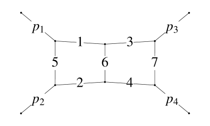
All planar two-loop diagrams that are required for the production of two off-shell vector bosons can be described by a single meta-graph shown in Figure 1. Three mappings, that define three distinct families of integrals, need to be considered:
-
1.
family P12 : ;
-
2.
family P13: ;
-
3.
family P23: .
For each of these families, we define a set of integrals that is closed under the application of integration-by-parts identities. Specifically,
| (8) |
and
| (9) |
Here, the exponents can take any integer values, with the restriction that and . These factors are used to represent irreducible numerators. For each of the three families, integration-by-parts identities can be used to express all the integrals of that type to a minimal set of (master) integrals. Our choice of master integrals can be found in Section 7. These master integrals satisfy differential equations in the external kinematic variables. In the next Section we discuss how such systems of equations can be solved.
3 Differential equations
In this Section we discuss how the master integrals can be calculated. To this end, we derive systems of differential equations for each of the above families. This is a relatively standard procedure, see e.g. kotikov ; remiddi and we do not discuss it further. When deriving differential equations we performed a reduction to master integrals using FIRE Smirnov:2008iw ; Smirnov:2013dia . We choose all master integrals to be dimensionless, such that they depend only on the three variables , and obtain
| (10) |
where or and is a vector of master integrals. The matrices contain simple rational functions. They satisfy the integrability conditions
| (11) |
for . The structure of the equations can be further clarified by writing them in the combined form
| (12) |
where the differential acts on and . For our choice of master integrals (see Section 7), the matrix can be written in the following way
| (13) |
where the are constant matrices, and the arguments of the logarithms , called letters, are simple functions of . We find
| (14) |
We call Eq. (3) the alphabet relevant to the functions . For example, in case of family P12, the first twelve of these letters are required. Eq. (12) makes it manifest that the analytic solution, to all orders in the expansion, can be written in terms of multiple polylogarithms defined by the alphabet (3). In general, the solution to Eq. (12) can be written in the elegant form
| (15) |
where refers to path ordering of the matrix exponential, and the integrals are Chen iterated integrals Chen:1977oja along the contour in the space of kinematical variables . The vector represents the boundary value at the base point of the contour . Eq. (15) is to be understood as a series expansion for small . The homotopy invariance of (15) allows for many equivalent representations of the same functions, corresponding to different choices and parametrizations of .333For a recent example in the context of Bhabha scattering, see Ref. Henn:2013woa . For this reason Eq. (15) is probably the most compact and invariant representation of the functions . However, for practical applications, we find it convenient to make a specific choice of the integration contour.
Indeed, the linearity of the alphabet allows us to write a simple representation of in terms of multiple polylogarithms. This can be thought of as a specific choice of the contour . Another way to arrive at such a solution is to integrate Eqs. (10) over one variable at a time. In the next Section, we will discuss this in more detail.
Note that singular points of the differential equations (12) can be read off from the alphabet (3). They correspond to special kinematic points such as singular limits, threshold or pseudo-threshold configurations of the multivalued functions . A useful feature of the differential equations is that they allow one to easily determine the behavior of close to singular points, and this is helpful in determining the boundary conditions Henn:2013nsa . A practical example of how this is done can be found in Section 5.
Finally, we wish to point out that the letters in Eq. (14) all have a definite sign in the physical regions. This means that all iterated integrals needed for calculating can be written in a manifestly real way, and imaginary parts appear only through explicit factors of . The latter come from the boundary conditions in the physical region.
4 Solution in terms of multiple polylogarithms
The vector of master integrals can be expanded in powers of ,
| (16) |
To construct a solution of the differential equation, we need to iteratively solve Eq. (10) order-by-order in dimensional-regularization parameter . Suppose the solution is constructed up to . The set of differential equations for is then
| (17) |
To find , we integrate the first equation over ; this determines the solution up to a function of
| (18) |
It follows from Eqs. (12),(13), and (3) that the integration kernels appearing on the right-hand side of Eq. (18) only contain terms of the form , for some ’s. Therefore, the integration over can be performed systematically provided that is written in terms of Goncharov polylogarithms
| (19) |
For the simplicity of integration, it is important to keep the same order of integration, e.g. always start with , for all the integrals that contribute to the vector . If this is not done consistently – so that integration variables also appear in indices of Goncharov polylogarithms in addition to their arguments – one has to use various identities between Goncharov polylogarithm to remedy this situation and enable the integration as in Eq. (19). Substituting the solution in Eq. (18) into the second term in Eq. (17), we find the differential equation for the function
| (20) |
where is a matrix related to the original matrix in a non-trivial way. Note, however, that this equation can only depend on the elements of the alphabet that are independent of ; this provides a non-trivial check of the consistency of reconstructed solutions. Integrating this equation over , we find
| (21) |
where is an arbitrary function of a single variable . Substituting Eq. (18) with from Eq. (21) into the third equation in Eq. (17), we find a differential equation for that is independent of and
| (22) |
The solution to this equation
| (23) |
is determined up to a constant of integration . This constant of integration has to be determined from the boundary conditions that we will discuss presently. Once is found, we employ the same strategy to obtain .
5 Boundary conditions in the physical region
It is common practice (see e.g. Refs. Gehrmann:2002zr ; tancredi ) that a solution to differential equations is first constructed in an unphysical region, where the solution is real and unique, and then properly continued into the physical region. We have found it difficult to follow this approach here. The reason has to do with the mapping from the kinematic variables and masses , where the analytic continuation is simple, to the variables. It is the non-linear nature of this mapping that makes it difficult to perform the proper analytic continuation once the result is written in variables. Because of that, we decided to perform computations directly in the physical region. Note that an analysis of master integrals for reported recently in Ref. tancredi arrives at a similar conclusion: all, but one, of the integrals described in that reference are obtained using analytic continuation, while the remaining integral is computed directly in the physical region since the analytic continuation becomes too cumbersome. We, however, decided in favor of a unified approach for computing all the integrals for planar graphs.
To understand how solutions in the physical region are constructed, we note that a Goncharov polylogarithm may develop an imaginary part when its argument is larger than at least one of the indices. Inspecting the alphabet in Eq. (14), it is easy to realize that in the kinematic region of interest, every entry in the alphabet is sign-definite. Therefore, upon integrating over , and from zero to their actual values, we can explicitly construct a real-valued solution, thereby by-passing all the subtleties related to analytic continuation of Goncharov polylogarithms. However, since in the physical region Feynman integrals do have imaginary parts, we should be able to get them in our approach as well and it is clear that, in case one has a sign-definite alphabet, imaginary parts can only appear through the boundary conditions.
To determine boundary conditions, we consider the limit , and . Physically, this limit corresponds to the production of two vector bosons, one with the mass and the other with the mass . The total energy squared of the collision is , which implies that the two vector bosons are at rest in the center-of-mass frame of the colliding partons. For two families, P12 and P13, the only singularities that are developed in this limit, are related to the mass of the lightest of the two vector bosons; for them, and can be set to one and the limit of small -values needs to be approached carefully. A typical behavior of an integral in that limit is , where is some integer. Unfortunately, for some integrals required for the family P23, the limit is also not smooth due to the appearances of the so-called double-parton scattering singularities Gaunt:2011xd . For such integrals, a typical asymptotic in the limit reads
| (24) |
where are integers. Our goal is to compute constants the to the relevant order in and then use them to construct solutions of differential equations as explained in the previous Section.
There are at least two ways to compute asymptotics in the required limits. One option is to simply take the limit in an integrand of a relevant Feynman integral. Since most of the integrals diverge in at least one of these limits, we need to resort to asymptotic expansions to evaluate them. To this end, one can use the strategy of expansion by regions Beneke:1997zp ; Smirnov:2002pj (for a recent review see Chapter 9 of Ref. Smirnov:2012gma ) and its implementation in an open computer code asy.m Pak:2010pt ; Jantzen:2012mw which is now included into FIESTA Smirnov:2013eza . To apply this code to a given Feynman integral, one has to specify the propagators, their powers and the limit of interest, by identifying the small parameter in the problem. As an output one obtains contributions of regions relevant for the given limit, in terms of Feynman-parametric integrals. Such integrals are further evaluated by the method of Mellin–Barnes representation Smirnov:1999gc ; Tausk:1999vh ; Smirnov:2012gma . In fact, for some of the master integrals of family P23, we considered two limits, and . When we evaluated asymptotics in the second limit, we used parametric integrals obtained after taking the first limit as an input for the second limit, also using the code asy.m.
An alternative, and in some cases simpler, way to get the boundary conditions for complicated integrals, is provided by the differential equations. To illustrate it, we consider a differential equation in the -variable for the box integral of the family P12. The definition of the integral can be found in the next Section. Writing the differential equation in the limit , we find
| (25) |
where ellipses stand for less singular terms. In limit, all the integrals in the family must have finite limits. The consistency of this requirement with Eq. (25) leads to a relation between different integrals
| (26) |
As can be seen from Section 7, where all master integrals are defined, the integrals are the two-loop two-point functions and is a relatively simple three-point function, whose limits are straightforward to obtain. We find
| (27) |
We then read off the limit of the integral from Eq. (26) implies
| (28) |
Finally, we note that the boundary conditions in the physical region for all the master integrals are reported in Section 7. To make sure that the boundary conditions are correct, we have often used both strategies described above to evaluate them. An agreement between these independent computations is a non-trivial check of the correctness of the boundary conditions.
6 Analytic continuation
In the previous Section, we described how we determined the boundary behavior of the integrals directly in the physical region, thereby avoiding the necessity of any analytic continuation. As we pointed out, the analytic continuation is not obvious to perform in the variables. The problem is that the change of variables Eq. (5) is non-linear. Therefore, our insistence on writing results in terms of Goncharov polylogarithms makes the analytic structure of the solution less obvious.
Here, we wish to show how the analytic continuation can be easily done in the language of Chen iterated integrals, in terms of the original variables, . We will take the integral family P23 as an example. This will also be a useful check of our results, since the boundary behavior for this integral family is particularly complicated in the physical region.
The integrals of family P23 depend on the variables . We can start from a non-physical region with . The physical region is then reached by analytically continuing to , keeping in mind the Feynman prescription. Note that such an analytic continuation is possible, since the integrals in the P23 family do not have discontinuities in the Mandelstam variable , so that the incorrect prescription for the Mandelstam variable , induced by the analytic continuation of , is not relevant.
We will discuss a single-parameter slice of the functions, which is obtained by fixing two Mandelstam variables and varying the remaining two. Specifically, we choose
| (29) |
A nice feature of this parametrization is that the alphabet (3) needed to describe the functions becomes simply
| (30) |
The boundary constants in the non-physical region are easily fixed. In fact, they can be obtained from the requirement that no branch cuts should start in that region. In the present case, the potential singularity at , cf. Eq. (30), must be spurious. Experience shows that such conditions usually allow one to determine all boundary constants without calculations Henn:2013tua ; Henn:2013nsa . The same is true here. For the basis choice made in Section 7, one easily sees that the boundary values at are given by
| (31) |
Here and are just the explicit values of trivial bubble-type integrals. They are given by
| (32) | ||||
| (33) |
Taking into account that
| (34) |
we see that after multiplying with , the expansion of these functions has uniform weight. This, together with the differential equations (12), shows that the solution has uniform weight in the expansion, to all orders in .
Let us now discuss the analytic continuation in to negative values of . The Feynman prescription implies that should have a small negative imaginary part. The alphabet in Eq. (30) indicates that poles in the complex plane are located at , and at infinity. As we discussed earlier, the pole at is spurious. There are branch cuts along the negative real axis, starting at , and possibly along the imaginary axis starting from .
It is now clear how to analytically continue to negative values of . We can choose a path below the negative real axis, but with , thereby avoiding branch cuts. Then we simply evaluate the Chen iterated path integral along this contour. We have done so for a path consisting of two segments, the first along the real axis from to , and the second along the semi-circle , with . In this way, we numerically verified the values for obtained in the physical region at . In terms of the variables of Eq. (5), this point corresponds to .
Given the simplicity of the alphabet (30) arising from the parametrization (29), it is also possible to perform the analytic continuation in a more algebraic way. Indeed, the terms that require analytic continuation are the ones that develop logarithmic singularities as . In the present case, functions corresponding to the alphabet (30) can be written as Goncharov polylogarithms with indices . The terms with logarithmic divergences are the ones with ’s at the rightmost entry. This behavior can be made manifest by using shuffle relations for iterated integrals, e.g.
| (35) |
and so on, where we explicitly see . The logarithmic terms are then analytically continued according to . In this way, one arrives at a representation valid for .
In summary, the formulation of Eq. (15) in terms of iterated path integrals has many conceptional advantages; here we exploited its manifest homotopy invariance in order to perform the analytic continuation. On the other hand, if one first fixes an integration contour, in order, for example, to obtain an expression in terms of Goncharov polylogarithms, one looses much of this flexibility.
7 Master integrals
For each family of integrals, the Mandelstam variables are given by , , . Their relation to the physical Mandelstam variables and the ensuing parametrization in terms of variables can be read off using the mapping just before Eq. (8) and Eqs. (1), (5).
When choosing the master integrals we followed the strategy proposed in Ref. jhenn to find master integrals having uniform weight. As guiding principles for finding such integrals we analyzed generalized unitarity cuts, as well as explicit (Feynman) parameter representations of the integrals. Technically this is very similar to the analysis of certain three-loop massless integrals studied in Refs. Henn:2013tua ; Henn:2013nsa . In fact, some of the two-loop integrals with two off-shell legs are contained in those three-loop integrals as subintegrals. For more detailed explanations and examples, see Section 2 of Ref. Henn:2013tua .
Below we present the master integrals, and the boundary conditions in the physical region that we used to evaluate them. For convenience, we re-scale and renormalize the master integrals. In particular, for the families P12 and P13 we choose master integrals to be , while for the family P23, we choose master integrals as . The normalization constant is
| (36) |
Furthermore, to present the master integrals and the results for the limits, we use the following notation
| (37) |
The pictures below are intended to give a general idea of how the corresponding master integrals look like, but obviously do not show doubled propagators or numerators and prefactors. Also, in some cases we chose linear combinations of integrals as master integrals, and in those cases only one representative figure is given.
The master integrals and their boundary asymptotic behaviour at the point for the family P12 read
The master integrals for the family P13 and their limits in the kinematic point read
Finally, for the family a convenient set of master integrals and the corresponding boundary conditions are
8 Checks of the results
In this Section, we describe some checks of our results. We begin by making a few nearly self-evident comments. First, we emphasize that all the integrals are computed using one and the same method. While this, obviously, does not guarantee that results are correct, it reduces the number of issues that can appear if every integral is computed with a new technique. Second, we stress that, once the choice of master integrals is made and suitable variables are found, the integration procedure is straightforward and can be thoroughly checked by differentiating the obtained result to ensure that it satisfies the original differential equations in variables. Unfortunately, this procedure does not check the boundary conditions which, therefore have to be checked in some other way.
As we already mentioned in the Introduction, when we require external masses to be equal , we obtain a class of integrals considered recently in Ref. tancredi . Using the results for the integrals appended to the arXiv submission of Ref. tancredi , we have compared numerical values for a large number of integrals that we compute in this paper with integrals computed in Ref. tancredi , finding perfect agreement.444 For integral , which corresponds to the integral of Ref. tancredi , in that reference should be . We thank L. Tancredi for clarifying this point to us. As another check, we have computed some of our integrals numerically using the new version of the program FIESTA Smirnov:2013eza , that is capable of calculating Feynman integrals in the physical region. A perfect agreement with our analytic result is found for a few randomly selected points.
Finally, a procedure of analytic continuation discussed in Sec. 6 can also be used to independently construct solutions in the physical region for integrals of the P23 family. As we explained there, that procedure can also be implemented by means of numerical integration over contour in the complex plane starting from a point in unphysical region where the boundary conditions are simple. We have checked that, for a randomly selected point, this procedure gives results for master integrals of family P23 that are in agreement with our analytic solutions.
9 Conclusions
In this paper we reported on the computation of all two-loop planar master integrals that are required to describe production of two off-shell vector bosons in hadron collisions. We constructed the differential equations for the carefully-chosen basis of master integrals following the strategy suggested in Ref. jhenn . We have computed boundary conditions for these integrals in the physical region and integrated them to obtain analytic results in terms of Goncharov polylogarithms. The results are fairly large. We note, however, that we did not try to simplify these results although such simplifications should be possible. Probably the most compact and flexible form can be achieved in terms of Chen iterated integrals, at the cost of giving up the feature of a linear parametrization. The matrices specifying them are included in the arXiv submission, as well as files with results for the integrals in terms of Goncharov polylogarithms.
The method for calculating multi-loop master integrals suggested in Ref. jhenn appears to be quite promising. We look forward to its application to even more complicated two-loop integrals and, in particular, to the non-planar ones required for the complete description of the off-shell production of two vector bosons at the LHC.
Acknowledgments
K.M. would like to thank Fabrizio Caola for many useful conversations. J.M.H. wishes to thank the organizers of RADCOR 2013, where a preliminary version of these results was presented, for their invitation. J.M.H. is supported in part by the DOE grant DE-SC0009988 and by the Marvin L. Goldberger fund. The work of K.M. is partially supported by US NSF under grants PHY-1214000 and by Karlsruhe Institute of Technology through its distinguished researcher fellowship program. The work of V.S. was supported by the Alexander von Humboldt Foundation (Humboldt Forschungspreis). We are grateful to the Institute for Theoretical Particle Physics (TTP) at Karlsruhe Institute of Technology where some of the results were obtained.
References
- (1) T. Gehrmann, L. Tancredi and E. Weihs, JHEP 1308, 070 (2013) [arXiv:1306.6344, arXiv:1306.6344 [hep-ph]].
- (2) See e.g. CMS notes CMS-PAS-SMP-12-016, CMS-PAS-SMP-13-01; CMS collaboration, Phys. Lett. B 721 (2013), 190.
- (3) ATLAS collaboration, Eur. Phys. J. C72 (2012), 2173, Phys. Rev. D 87 (2013), 113001.
- (4) L. Dixon, Z. Kunszt and A. Signer, Nucl. Phys. B531 (1998), 3.
- (5) L. Dixon, Z. Kunszt and A. Signer, Phys. Rev. D60 (1999), 114037.
- (6) A. Bierweiler, T. Kasprzik and J. H. Kühn, JHEP 1312, 071 (2013) [arXiv:1305.5402 [hep-ph]].
- (7) S. Dawson, I.M. Lewis and M. Zeng, Phys. Rev. D88 (2013), 054028.
- (8) P. Nason and G. Zanderighi, arXiv:1311.1365.
- (9) F. Caola and K. Melnikov, Phys. Rev. D 88, 054024 (2013) [arXiv:1307.4935 [hep-ph]].
- (10) J. M. Campbell, R. K. Ellis and C. Williams, arXiv:1311.3589 [hep-ph].
- (11) J. Currie, A. Gehrmann-De Ridder, E. W. N. Glover and J. Pires, JHEP 1401, 110 (2014) [arXiv:1310.3993 [hep-ph]].
- (12) A. Gehrmann-De Ridder, T. Gehrmann, E. W. N. Glover and J. Pires, Phys. Rev. Lett. 110, no. 16, 162003 (2013) [arXiv:1301.7310 [hep-ph]].
- (13) M. Czakon, P. Fiedler and A. Mitov, Phys. Rev. Lett. 110, 252004 (2013) [arXiv:1303.6254 [hep-ph]].
- (14) P. Baernreuther, M. Czakon and A. Mitov, Phys. Rev. Lett. 109, 132001 (2012) [arXiv:1204.5201 [hep-ph]].
- (15) R. Boughezal, F. Caola, K. Melnikov, F. Petriello and M. Schulze, JHEP 1306, 072 (2013) [arXiv:1302.6216 [hep-ph]].
- (16) F. Tkachov, Phys. Lett. B100 (1981), 65; K.G. Chetyrkin and F. Tkachov, Nucl. Phys. B192 (1981), 159.
- (17) A. Kotikov, Phys. Lett. B254 (1991), 158.
- (18) E. Remiddi, Nuovo Cimento A110 (1997), 1435.
- (19) A. V. Smirnov, JHEP 0810 (2008) 107 [arXiv:0807.3243 [hep-ph]].
- (20) A. V. Smirnov and V. A. Smirnov, Comput. Phys. Commun. 184 (2013) 2820 [arXiv:1302.5885 [hep-ph]].
- (21) M. Caffo, H. Czyz, S. Laporta and E. Remiddi, Nuovo Cimento A111 (1998), 365.
- (22) T. Gehrmann and E. Remiddi, Nucl. Phys. B580 (2000), 485.
- (23) J.M. Henn, Phys. Rev. Lett. 110 (2013).
- (24) J. M. Henn, A. V. Smirnov and V. A. Smirnov, JHEP 1307 (2013) 128 [arXiv:1306.2799 [hep-th]].
- (25) J. M. Henn and V. A. Smirnov, JHEP 1311 (2013) 041 [arXiv:1307.4083].
- (26) J. M. Henn, A. V. Smirnov and V. A. Smirnov, arXiv:1312.2588 [hep-th].
- (27) V. A. Smirnov, Phys. Lett. B 460 (1999) 397 [hep-ph/9905323].
- (28) V. A. Smirnov and O. L. Veretin, Nucl. Phys. B 566 (2000) 469 [hep-ph/9907385].
- (29) J. B. Tausk, Phys. Lett. B 469 (1999) 225 [hep-ph/9909506].
- (30) C. Anastasiou, T. Gehrmann, C. Oleari, E. Remiddi and J. B. Tausk, Nucl. Phys. B 580 (2000) 577 [hep-ph/0003261].
- (31) T. Gehrmann and E. Remiddi, Nucl. Phys. B601 (2001), 248.
- (32) T. Gehrmann and E. Remiddi, Nucl. Phys. B601 (2001), 287.
- (33) C. Papadopoulos, hep-ph/1401.6057.
- (34) K. -T. Chen, Bull. Am. Math. Soc. 83, 831 (1977).
- (35) T. Gehrmann and E. Remiddi, Nucl. Phys. B 640, 379 (2002) [hep-ph/0207020].
- (36) J. R. Gaunt and W. J. Stirling, JHEP 1106, 048 (2011) [arXiv:1103.1888 [hep-ph]].
- (37) M. Beneke and V. A. Smirnov, Nucl. Phys. B 522 (1998) 321 [hep-ph/9711391].
- (38) V. A. Smirnov, Springer Tracts Mod. Phys. 177 (2002) 1.
- (39) V. A. Smirnov, Springer Tracts Mod. Phys. 250 (2012) 1.
- (40) A. Pak and A.V. Smirnov, Eur. Phys. J. C 71 (2011) 1626 [arXiv:1011.4863 [hep-ph]].
- (41) B. Jantzen, A. V. Smirnov and V. A. Smirnov, Eur. Phys. J. C 72 (2012) 2139 [arXiv:1206.0546 [hep-ph]].
- (42) A. V. Smirnov, arXiv:1312.3186 [hep-ph].