Effective Lagrangian for Nonrelativistic Systems

Abstract

The effective Lagrangian for Nambu-Goldstone bosons (NGBs) in systems without Lorentz invariance has a novel feature that some of the NGBs are canonically conjugate to each other, hence describing $1$ dynamical degree of freedom by two NGB fields. We develop explicit forms of their effective Lagrangian up to the quadratic order in derivatives. We clarify the counting rules of NGB degrees of freedom and completely classify possibilities of such canonically conjugate pairs based on the topology of the coset spaces. Its consequence on the dispersion relations of the NGBs is clarified. We also present simple scaling arguments to see whether interactions among NGBs are marginal or irrelevant, which justifies a lore in the literature about the possibility of symmetry breaking in $1+1$ dimensions.

I Introduction

In studies of any macroscopic physical systems, the behavior of the system at low temperatures, small energies, and long distances is determined predominantly by microscopic excitations with small or zero gap. It is, hence, important to develop a general theory to discuss gapless excitations. Barring special reasons, however, we generally do not expect any gapless degrees of freedom in a given system. The important exceptions are (1) a Fermi liquid with the Fermi level within a continuous band, (2) second-order phase transitions with scale (and often conformal) invariance, (3) states protected by topological reasons such as edge states of topological insulators or quantum Hall states, and (4) Nambu-Goldstone bosons (NGBs) of spontaneous symmetry breaking. The first three cases are discussed extensively in the literature. We focus on the last case in this paper because a general theory, so far, has surprisingly been lacking, despite its importance and long history.

Spontaneously broken symmetry is a common theme through all areas of physics. The examples are numerous: Bose-Einstein condensates of cold atoms, superfluids of ⁴He or ³He, crystal lattices, neutron stars, ferromagnets, anti-ferromagnets, liquid crystals, chiral symmetry in QCD, and cosmic inflation. The universal feature is that it guarantees the existence of gapless excitations when the relevant symmetries are continuous. Once promoted to gauge symmetries, it is the basis to discuss superconductivity, the Englert-Bourt-Higgs mechanism, and cosmic strings. The crucial question is the following: What is the general theory that can describe the number of NGB degrees of freedom, and their dispersion relations, their interactions among each other and to other degrees of freedom? Ideally, the theory does not depend on specifics of a given system or perturbation theory but is rather determined by symmetries alone, so that it is applicable even when the system is strongly coupled or we lack understanding of the microscopic description.

In systems with Lorentz invariance, the general theory has already been established back in 1960’s by the celebrated Nambu-Goldstone theorem Nambu and Jona-Lasinio (1961); Goldstone (1961); Goldstone et al. (1962) and later with “phenomenological Lagrangians” by Callan, Coleman, Wess, and Zumino Coleman et al. (1969); Callan et al. (1969). It is important to formulate the theory using Lagrangians because a Lagrangian is a self-contained package to describe a system. It determines the degrees of freedom, equations of motion, Noether currents for symmetries, and commutation relations and provides the basis for perturbation theory using Feynman diagrams and many non-perturbative methods based on path integrals. In comparison, the Hamiltonian formalism Hohenberg and Halperin (1977); Mazenko (2006) requires additional input: what the degrees of freedom are and what their commutation relations (or Poisson brackets) are. Especially when at least one of these two is not clear at the beginning of the discussion, which turns out to be the case for our purposes, the Lagrangian formulation is essential.

However, many systems we are interested in are not Lorentz invariant. A finite temperature violates Lorentz invariance because the Boltzmann weight depends on the energy, which is the time component of the energy-momentum four-vector and hence requires a specific choice of the reference frame. A chemical potential needed to describe systems with finite densities couples to the charge density, which is also the time component of a conserved four-current. Often, the surrounding environment violates Lorentz invariance as well. In all of these cases, rotational invariance may still be present, while Lorentz invariance is certainly not there.

It is, therefore, of foremost importance to develop a general theory of NGBs based on symmetry principles alone without assuming Lorentz invariance. We develop such a theory in this paper.

NGBs without Lorentz invariance have been discussed for their obvious importance, as discussed above. The nonrelativistic  analog of one aspect of the NG theorem, that which ensures the appearance of at least one NGB, was already discussed back in the 1960s Lange (1965, 1966); Guralnik et al. (1968); Brauner (2010a). However, the number and the dispersion of the NGBs have only been studied on a case-by-case basis until quite recently.

The Nambu-Goldstone theorem says there must be one gapless excitation for every broken-symmetry generator, assuming Lorentz invariance. Moreover, Lorentz invariance constrains the dispersion relation for gapless excitation to be $\omega=ck$, where $c$ is the speed of light.

However, these predictions are known to be false in systems without Lorentz invariance. A classic example is a ferromagnet. When spins line up macroscopically due to the nearest-neighbor interaction, it spontaneously breaks the $\text{SO}(3)$ spin-rotational symmetry with three generators down to the unbroken $\text{SO}(2)$ axial symmetry with only one generator. Despite the two spontaneously broken symmetries, the ferromagnet exhibits only one NGB. Moreover, its dispersion is quadratic rather than linear. In contrast, an antiferromagnet supports two NGBs with a linear dispersion, although it shows the same symmetry-breaking pattern $\text{SO}(3)\rightarrow\text{SO}(2)$.

More recent examples appeared in relativistic field theories with nonzero chemical potentials, where examples of an “abnormal number of Nambu-Goldstone bosons” are identified in many contexts Miransky and Shovkovy (2002); Schäfer et al. (2001); Blaschke et al. (2004); He et al. (2006); Ebert et al. (1993, 2005); Buchel et al. (2007). Also, spinor Bose-Einstein condensates in cold atom systems added a number of new examples and realized some of them in the actual experiments Kawaguchi and Ueda (2012); Stamper-Kurn and Ueda (2013). The dispersion of the softest NGB immediately modifies the thermodynamic property of the system at a low temperature. For example, the low-temperature heat capacity behaves as $C(T)\propto T^{d/z}$ for the NGB with the dispersion $\omega\propto k^{z}$ in $d+1$ dimensions. In general, the low-energy dynamics of systems with spontaneous symmetry breaking is governed by NGBs, and hence, it is clearly important to establish a general theorem that predicts the correct number, dispersion, and interactions of NGBs.

In their pioneering work Nielsen and Chadha (1976), Nielsen and Chadha established an inequality that relates the number of NGBs to their dispersion relations. In their approach, NGBs are classified as type-I (type-II) if their dispersion in the long-wavelength limit behaves as $\omega\propto k^{2n-1}$ ($\omega\propto k^{2n}$). Based on the analytic property of correlation functions, Nielsen and Chadha proved that the number of type-I NGBs plus twice the number of type-II NGBs is greater than or equal to the number of broken-symmetry generators. Note that their conclusion is merely an inequality, and hence, it does not give any lower or upper bound for each type of NGB. Also, their classification breaks down when the dispersion is anisotropic, e.g., $\omega\propto\sqrt{(k_{x})^{2}+C(k_{y})^{4}}$. (See Sec. VI.1 for an example.)

In a relatively recent paper, Schäfer et al. Schäfer et al. (2001) pointed out the importance of expectation values of the commutators of the broken generators in reducing the number of NGBs. They showed that the number of NGBs must be equal to the number of broken generators if $\langle[Q_{a},Q_{b}]\rangle=0$ for all combinations of broken generators. Although their argument is physically plausible, it contains a few questionable points. They identified the NG state associated with the charge $Q_{a}$ as $Q_{a}|\Psi_{0}\rangle$ ($|\Psi_{0}\rangle$ is the quantum many-body ground state) and discussed the possibility of linear dependence among such vectors. However, it is well known that, once symmetries are spontaneously broken, broken generators themselves are ill defined. We should rather use commutation relations of generators with other local quantities.

Nambu Nambu (2004, 2005) was probably the first to obtain the correct insight into this problem. He observed that the nonzero expectation value $\langle[Q_{a},Q_{b}]\rangle$ makes zero modes associated with these generators canonically conjugate to each other, and hence, the number of NGBs is reduced by 1 per such a pair. However, he did not prove this claim on general grounds.

With these previous works in mind, the current authors unified all of the above observations into a simple and well-defined form by proving them using field theory Watanabe and Murayama (2012):

$$n_{\text{A}} = \text{dim}\,G/H-\text{rank}\rho,$$ (1)

$$n_{\text{B}} = \frac{1}{2}\text{rank}\rho,$$ (2)

$$n_{\text{NGB}} = \text{dim}\,G/H-\frac{1}{2}\text{rank}\rho,$$ (3)

$$n_{\text{A}}+2n_{\text{B}} = \text{dim}\,G/H,$$ (4)

$$i\rho_{ab} \equiv \langle[Q_{a},j_{b}^{0}(0)]\rangle.$$ (5)

Equation (3) was conjectured earlier in Ref. Watanabe and Brauner (2011) and was also obtained independently in Ref. Hidaka (2013). Here, $n_{\text{A}}$, $n_{\text{B}}$ represent the numbers of type-A, B NGBs, respectively, and $n_{\text{NGB}}\equiv n_{\text{A}}+n_{\text{B}}$ is the total number of NGBs. Equations (3) and (4) follow from Eqs. (1) and (2). $j_{a}^{\mu}(x)$ is the conserved current associated with a broken charge $Q_{a}=\int\mathrm{d}^{d}x\,j_{a}^{0}(x)$. The Lie group $G$ represents the original symmetry of the system, and $H$ is its unbroken subgroup, so that $\text{dim}\,G/H$ represents the number of broken-symmetry generators. Clearly, the symmetry-breaking pattern $G\rightarrow H$ is not sufficient to fix the number of NGBs, and we need additional information [the matrix $\rho$ in Eq. (5)] about the ground state.

The definitions of type-A, B NGBs are not based on their dispersion relations but on their symplectic structure, as we will discuss in detail later. For now, we just note that, generically, type-A NGBs have a linear dispersion and type-B NGBs have a quadratic dispersion, but there are exceptions. Therefore, Eq. (4) can be understood as the equality version of the Nielsen-Chadha theorem for most cases.

The above-explained theorem by Schäfer et al. can also be understood as the special case where the matrix $\rho$ vanishes, and hence, $n_{\text{NGB}}=\text{dim}\,G/H$ from Eq. (3). The matrix $\rho$ must always vanish in the Lorentz-invariant case, because $[Q_{a},j_{b}^{0}(\vec{x},t)]=if_{ab}^{\phantom{ab}c}j_{c}^{0}(\vec{x},t)$ in the absence of central extensions and $j_{c}^{\mu}(0)$ is a Lorentz vector, which cannot have an expectation value without breaking the Lorentz symmetry.

In order to prove the counting rule of NGBs and clarify their dispersion relations, we develop the nonrelativistic analog of the “phenomenological Lagrangian” à la Refs. Coleman et al. (1969); Callan et al. (1969), following Leutwyler’s works Leutwyler (1994a, b). We derive an explicit expression of the effective Lagrangian for a general symmetry breaking-pattern $G\rightarrow H$. In this process, we find a set of terms that have not been taken into account in the literature.

This fully nonlinear effective Lagrangian contains only a few parameters that play the role of coupling constants between NGBs. By analyzing the scaling law of the dominant interaction, we discuss the stability of the symmetry-broken ground state. In sufficiently high dimensions, the system is essentially free, as expected. However, it turns out that, in general, internal symmetries can be spontaneously broken even in $1+1$ dimensions. This is one of the aspects enriched by the absence of Lorentz invariance — in a Lorentz-invariant theory, the well-known Coleman theorem Coleman (1973) prohibits that possibility.

The explicit form of the effective Lagrangian leads to another nontrivial prediction, that is, a no-go theorem for a certain number of type-A and type-B NGBs. One might think that any combination of $n_{\text{A}}$ and $n_{\text{B}}$ subject to Eq. (4) should be possible. However, for given $G$ and $H$, possibilities are quite restricted, because type-B NGBs are described by symplectic homogeneous spaces, which are special types of coset spaces that admit the so-called Kähler structure, if $G$ is semisimple. We will discuss how the possible numbers for type-A and type-B can be completely enumerated for any given $G$ and $H$.

This paper is organized as follows. In Sec. II, we discuss the most general form of the effective Lagrangian for nonrelativistic systems and derive differential equations for the coefficients appearing in the effective Lagrangians by paying careful attention to the gaugeability of the symmetry $G$. We present an analytic solution of the differential equations in terms of the Maurer-Cartan form in Sec. III. We also clarify the obstacle to gauge Wess-Zumino-Witten terms and algebras with central extensions. Analyzing the free part of our effective Lagrangian, we prove the counting rule in Sec. IV and derive their dispersion in Sec. V. We discuss the interaction effect and spontaneous symmetry breaking in $1+1$ dimensions in Sec. VI.

In Sec. VII, we present the mathematical foundation of the canonically conjugate (presymplectic) structure among some NGBs. With this preparation, we completely classify the presymplectic structure and prove a no-go theorem that prohibits a certain combination of type-A and type-B NGBs in Sec. VIII. It is followed by concrete demonstration thorough familiar examples in Sec. IX.

We will not discuss the counting of NGBs associated to spacetime symmetries. For those symmetries, the number of NGBs is reduced not only by forming canonically conjugate pairs but also by other mechanisms, e.g., linear dependence among conserved currents. Hence the above counting rule does not hold. See Refs. Low and Manohar (2002); Watanabe and Murayama (2013); Hayata and Hidaka (2014); Brauner and Watanabe (2014) for more details. Nevertheless, we explain how to impose the Galilean symmetry, if it exists, on the effective Lagrangian in Sec. X.

For the reader’s convenience, we present a pedagogical introduction to the cohomology of Lie algebra in Appendix A. We also review how to couple matter fields to NGBs in Appendix B. Finally, we clarify a confusion in the existing literature on the relation between type-B NGBs and the time-reversal symmetry in Appendix C.

II Effective Lagrangian for nonrelativistic systems

In this section, we describe the general effective Lagrangian for NGBs on the coset space $G/H$. One way of deriving the effective Lagrangian is to integrate out all high-energy modes from an assumed microscopic model. However, there is an alternative universal approach, which is more convenient for our general discussion. Namely, we simply write down the most general Lagrangian that has the assumed symmetry Weinberg (1995). Clearly, the Lagrangian derived from the former approach always falls into this general form, and all terms allowed by symmetry should be generated at least in the process of renormalization.

We assume rotational invariance of space, but no Lorentz invariance. There are terms that have not been considered traditionally. The Lagrangian is considered to be an expansion in the number of derivatives to study long-range and low-energy excitations of the system. We restrict ourselves to terms up to second order in derivatives because they are sufficient to read off the number and dispersion relations of NGBs for most purposes. To work out symmetry requirements on the functional forms of each term in the Lagrangian, differential forms turn out to be very useful.

II.1 Coset space

Suppose that the symmetry group $G$ of a microscopic Lagrangian is spontaneously broken down to its subgroup $H$. The set of the degenerate ground states forms the coset space $G/H$. The low-energy effective Lagrangian is the nonlinear sigma model with the target space $G/H$. We consider only exact symmetries (i.e., without anomalies or explicit breaking). We also set $\hbar=1$ throughout the paper. Except in Sec. X and a few examples in VI.1, we assume that $G$ and $H$ are compact Lie groups for internal symmetries.

Let $\pi^{a}$ ($a=1,\ldots,\text{dim}\,G/H$) be a local coordinate of $G/H$. By definition, the number of fields always equals the number of broken generators $\text{dim}\,G/H$. Every point on this space is equivalent, and we pick the origin $\pi^{a}=0$ as our ground state. The NG field $\pi^{a}(\vec{x},t)$ is a map $\pi:\mathbb{R}^{d+1}\rightarrow G/H$. ($d$ is the spatial dimension.)

$\pi^{a}$’s form a nonlinear realization of $G$. They transform under $\epsilon^{i}Q_{i}$ as

$$\delta_{\epsilon}\pi^{a}=\epsilon^{i}h^{a}_{i}(\pi).$$ (6)

Generators $h_{i}^{a}(\pi)$ can be viewed as vector fields on $G/H$

$$h_{i}(\pi)=h_{i}^{a}(\pi)\partial_{a},\quad\partial_{a}\equiv\frac{\partial}{\partial\pi^{a}},$$ (7)

and their Lie bracket is identified with the commutation relation

$$[h_{i},h_{j}]\equiv(h_{i}^{b}\partial_{b}h_{j}^{a}-h_{j}^{b}\partial_{b}h_{i}^{a})\partial_{a}=f_{ij}^{\phantom{ij}k}h_{k}.$$ (8)

Here, $i,j,k,\ldots$ refer to generators of $G$.

In general, we will look for the most general Lagrangian $\mathcal{L}_{\text{eff}}(\pi,\dot{\pi},\nabla_{r}\pi,\ddot{\pi}^{a},\nabla_{r}\dot{\pi}^{a},\nabla_{r}\nabla_{s}\pi^{a},\ldots)$ that only changes by total derivatives under the transformation in Eq. (6). A particularly useful choice of the nonlinear realization is given by the Callan-Coleman-Wess-Zumino coset construction Coleman et al. (1969); Callan et al. (1969), which we introduce in Sec. III.1.

If the symmetry can be gauged, parameters of symmetry transformations are local $\epsilon^{i}(x)$, and we may introduce gauge fields that transform as

$$\delta_{\epsilon}A^{i}_{\mu}(x) =[\mathcal{D}_{\mu}\epsilon(x)]^{i}=\nabla_{\mu}\epsilon^{i}(x)+f_{jk}^{\phantom{jk}i}A^{j}_{\mu}\epsilon^{k}(x),$$ (9)

where $A_{\mu}^{i}=(A_{t}^{i},\vec{A}^{i})$ and $\nabla_{\mu}=(\nabla_{t},\vec{\nabla})$. However, not all symmetries can be gauged. Such examples are discussed in Sec. III.5. In order to keep the full generality, we first proceed without gauging the symmetry. We will then discuss the local symmetry and clarify the obstruction.

II.2 Derivative expansion and symmetry requirements

We postulate the locality of the microscopic Lagrangian; i.e., it does not include terms containing fields at two separated points $(\vec{x},t)$ and $(\vec{x}^{\prime},t^{\prime})$. Then, the effective Lagrangian obtained by integrating our higher-energy modes should stay local .

To study the low-energy structure of the effective Lagrangian systematically, we employ the derivative expansion. Namely, we expand the Lagrangian in the power series of the time derivative $\nabla_{t}$ and the spatial derivative $\nabla_{r}$ ($r,s=1,\ldots,d$). We do not require Lorentz invariance but we do require spatial rotational symmetry. Because of the lack of the Lorentz invariance, the space and time derivatives may scale differently. For example, $O(\nabla_{t}^{2})$ and $O(\nabla_{r}^{2})$ may not be of the same order in a derivative expansion. We also assume the broken symmetries are internal symmetries, and hence the NG fields are spacetime scalars.

To avoid possible confusion, we use $\nabla_{r}$ to represent the spatial derivative and $\nabla_{t}$ or a“dot” to represent the time derivative. $\partial_{a}\equiv\partial/\partial\pi^{a}$ ($a=1,\ldots,\text{dim}\,G/H$) refers to the derivatives with respect to internal coordinates of $G/H$.

With these cautions in mind, we find the most general form of the effective Lagrangian Leutwyler (1994a) up to the second order in derivatives in $3+1$ dimensions and above:

$$\mathcal{L}_{\mathrm{eff}}=c_{a}(\pi)\dot{\pi}^{a}+\frac{1}{2}\bar{g}_{ab}(\pi)\dot{\pi}^{a}\dot{\pi}^{b}-\frac{1}{2}g_{ab}(\pi)\vec{\nabla}\pi^{a}\cdot\vec{\nabla}\pi^{b}.$$ (10)

In $1+1$ dimensions, there is no spatial rotation, and therefore, we can add three more terms:

$$\tilde{c}_{a}(\pi)\nabla_{x}\pi^{a}+\tilde{g}_{ab}(\pi)\dot{\pi}^{a}\nabla_{x}\pi^{b}+\tilde{b}_{ab}(\pi)\dot{\pi}^{a}\nabla_{x}\pi^{b}.$$ (11)

Also, in $2+1$ dimensions, there is an invariant antisymmetric tensor $\epsilon^{rs}$, and therefore,

$$-\frac{1}{2}b_{ab}(\pi)\epsilon^{rs}\nabla_{r}\pi^{a}\nabla_{s}\pi^{b}$$ (12)

is allowed. $g_{ab}$, $\bar{g}_{ab}$, and $\tilde{g}_{ab}$ are symmetric, and $b_{ab}$ and $\tilde{b}_{ab}$ are antisymmetric with respect to $a$ and $b$. Terms that contain $\ddot{\pi}^{a}$, $\nabla_{r}\dot{\pi}^{a}$, and $\nabla_{r}\nabla_{s}\pi^{a}$ can be brought to the above form by integration by parts.

We discuss that the $c_{a}(\pi)$ term can be interpreted as the Berry phase in Sec. III.6. The terms in Eqs. (11) and (12) have not been taken into account in Ref. Leutwyler (1994a). However, they preserve the assumed rotational invariance in $1+1$ or $2+1$ dimensions and therefore are allowed, in general. We present an example of them in Sec. III.2.4.

There are two subtleties about the terms $\tilde{c}_{a}(\pi)$ and $b_{ab}(\pi)$. First, the energy functional derived by the Lagrangian (10) plus the terms in Eq. (11) is

$$\int\mathrm{d}^{d}x\left[\frac{1}{2}\bar{g}_{ab}\dot{\pi}^{a}\dot{\pi}^{b}+\frac{1}{2}g_{ab}\nabla_{x}\pi^{a}\nabla_{x}\pi^{b}-\tilde{c}_{a}\nabla_{x}\pi^{a}\right],$$ (13)

In the Fourier space, the second term is $O(k_{x}^{2})$ and the last term is $O(k_{x})$. Thus, the energy is minimized by a nonzero $k_{x}$ and the translational symmetry will be spontaneously broken. Although the $O(k_{x})$ term and the $O(k_{x}^{2})$ term balance against each other, this solution may still be consistent with the derivative expansion if the coefficient of the $O(k_{x})$ term is somehow small. Since our main interest is in the situation with unbroken translational symmetry, we will not discuss the consequences of this term any further.

Second, $\tilde{c}_{a}(\pi)$ and $b_{ab}(\pi)$ cannot be Wess-Zumino-Witten type terms (see Sec. III.5). They appear in the energy functional, unlike the terms $c_{a}(\pi)$ and $\tilde{b}_{ab}(\pi)$, which are linear in the time derivative. In order for the energy to be well-defined, $\int\mathrm{d}x\,\tilde{c}_{a}(\pi)\nabla_{x}\pi^{a}$ and $\int\mathrm{d}^{2}x(1/2)b_{ab}(\pi)\epsilon^{rs}\nabla_{r}\pi^{a}\nabla_{s}\pi^{b}$ cannot possess the ambiguity of $2\pi k$ ($k\in\mathbb{Z}$). Another way of putting it is the Wick rotation. In the case of $c_{a}(\pi)$ and $\tilde{b}_{ab}(\pi)$, the factor of $i$ from their time derivative $\partial_{t}$ and from $\mathrm{d}t$ in the integral measure cancel each other out under the Wick rotation and the ambiguity of the action remains to be an integer multiple of $2\pi i$. However, if either $\tilde{c}_{a}(\pi)$ or $b_{ab}(\pi)$ were a Wess-Zumino-Witten-type term, the absolute value of the path-integral weight would not be well defined after the Wick rotation due to the lack of a time derivative.

Our task is to determine coefficients $c_{a}(\pi)$, $\tilde{c}_{a}(\pi)$, $g_{ab}(\pi)$, $\bar{g}_{ab}(\pi)$, $\tilde{g}_{ab}(\pi)$, $b_{ab}(\pi)$, and $\tilde{b}_{ab}(\pi)$ by imposing the global symmetry $G$.

Under global transformation (6), the first term of the Lagrangian (10) transforms as

$$\delta_{i}(c_{a}\dot{\pi}^{a})=(h_{i}^{b}\partial_{b}c_{a}+c_{b}\partial_{a}h_{i}^{b})\dot{\pi}^{a}.$$ (14)

By requiring that this combination is a total derivative $\nabla_{t}(e_{i}+c_{a}h_{i}^{a})$, we find

$$(\partial_{b}c_{a}-\partial_{a}c_{b})h_{i}^{b}=\partial_{a}e_{i}.$$ (15)

Similarly, for $\tilde{c}_{a}(\pi)$, $b(\pi)$, and $\tilde{b}(\pi)$, we have

$$(\partial_{b}\tilde{c}_{a}-\partial_{a}\tilde{c}_{b})h_{i}^{b} = \partial_{a}\tilde{e}_{i},$$ (16)

$$(\partial_{a}b_{bc}+\partial_{b}b_{ca}+\partial_{c}b_{ab})h_{i}^{c} = \partial_{a}e_{ib}^{\prime}-\partial_{b}e_{ia}^{\prime},$$ (17)

$$(\partial_{a}\tilde{b}_{bc}+\partial_{b}\tilde{b}_{ca}+\partial_{c}\tilde{b}_{ab})h_{i}^{c} = \partial_{a}\tilde{e}_{ib}^{\prime}-\partial_{b}\tilde{e}_{ia}^{\prime}.$$ (18)

Here, $\tilde{e}_{i}(\pi)$, $e_{ia}^{\prime}(\pi)$, and $\tilde{e}_{ia}^{\prime}(\pi)$ are also related to the change of the Lagrangian by total derivatives $\nabla_{t}(\tilde{e}_{i}+\tilde{c}_{a}h_{i}^{a})$, $\nabla_{r}[\epsilon^{rs}(e_{ib}^{\prime}+b_{ab}h_{i}^{a})\nabla_{s}\pi^{b}]$, and $\nabla_{t}[(\tilde{e}_{ib}^{\prime}+\tilde{b}_{ab}h_{i}^{a})\nabla_{x}\pi^{b}]-\nabla_{x}[(\tilde{e}_{ib}^{\prime}+\tilde{b}_{ab}h_{i}^{a})\dot{\pi}^{b}]$.

In contrast, the second term of Eq. (10) must be invariant by itself; i.e., they cannot change by a surface term.

$$\delta_{i}\left(g_{ab}\vec{\nabla}\pi^{a}\cdot\vec{\nabla}\pi^{b}\right)$$

$$=(h_{i}^{c}\partial_{c}g_{ab}+g_{cb}\partial_{a}h_{i}^{c}+g_{ac}\partial_{b}h_{i}^{c})\vec{\nabla}\pi^{a}\cdot\vec{\nabla}\pi^{b}=0.$$ (19)

If the left hand side of Eq. (19) were a total derivative $\nabla_{r}\Lambda_{i}^{r}$, $\Lambda_{i}^{r}$ would take the form $f_{ia}(\pi)\nabla_{r}\pi^{a}$. However, $\nabla_{r}\Lambda_{i}^{r}$ then contains a term $\nabla_{r}^{2}\pi^{a}$, which was absent in Eq. (19). Thus, $\Lambda_{i}^{r}$ has to be $0$. Therefore,

$$h_{i}^{c}\partial_{c}g_{ab}+g_{cb}\partial_{a}h_{i}^{c}+g_{ac}\partial_{b}h_{i}^{c}=0.$$ (20)

The same equation holds for $\bar{g}_{ab}(\pi)$ and $\tilde{g}_{ab}(\pi)$:

$$h_{i}^{c}\partial_{c}\bar{g}_{ab}+\bar{g}_{cb}\partial_{a}h_{i}^{c}+\bar{g}_{ac}\partial_{b}h_{i}^{c} = 0,$$ (21)

$$h_{i}^{c}\partial_{c}\tilde{g}_{ab}+\tilde{g}_{cb}\partial_{a}h_{i}^{c}+\tilde{g}_{ac}\partial_{b}h_{i}^{c} = 0.$$ (22)

In summary, coefficients in the effective Lagrangian must obey the differential equations (15)–(18) and (20)–(22) in order that the Lagrangian has the symmetry $G$. We also have to derive the differential equations for $e_{i}(\pi)$, $\tilde{e}_{i}(\pi)$, $e_{ia}^{\prime}(\pi)$, and $\tilde{e}_{ia}^{\prime}(\pi)$ and it can easily be done by using the mathematical technique we introduce in the next section.

II.3 Geometric derivation

II.3.1 Equations on $c(\pi)$’s and $g(\pi)$’s

Here, we rederive the above differential equations by using differential geometry, to set up notations and introduce useful mathematical tools for later calculation. The terms in the effective Lagrangian can be viewed as one-forms

$$c(\pi) = c_{a}(\pi)\mathrm{d}\pi^{a},$$ (23)

$$\tilde{c}(\pi) = \tilde{c}_{a}(\pi)\mathrm{d}\pi^{a},$$ (24)

symmetric tensors

$$g(\pi)=g_{ab}(\pi)\mathrm{d}\pi^{a}\otimes\mathrm{d}\pi^{b},$$ (25)

$$\bar{g}(\pi)=\bar{g}_{ab}(\pi)\mathrm{d}\pi^{a}\otimes\mathrm{d}\pi^{b},$$ (26)

$$\tilde{g}(\pi)=\tilde{g}_{ab}(\pi)\mathrm{d}\pi^{a}\otimes\mathrm{d}\pi^{b},$$ (27)

and two-forms

$$b(\pi)=b_{ab}(\pi)\mathrm{d}\pi^{a}\wedge\mathrm{d}\pi^{b},$$ (28)

$$\tilde{b}(\pi)=\tilde{b}_{ab}(\pi)\mathrm{d}\pi^{a}\wedge\mathrm{d}\pi^{b}$$ (29)

on the manifold $G/H$. Note that $c(\pi)$, $\tilde{c}(\pi)$, $b(\pi)$, and $\tilde{b}(\pi)$ do not necessarily exist globally.

In the following, we use Cartan’s magic formula that relates the Lie derivative $\mathscr{L}_{X}$, the exterior derivative $\mathrm{d}$, and the interior product $\mathrm{i}_{X}$:

$$\mathscr{L}_{X}\omega=(\mathrm{d}\,\mathrm{i}_{X}+\mathrm{i}_{X}\mathrm{d})\omega.$$ (30)

Equation (30) is true for arbitrary forms $\omega$ and vector fields $X$ Nakahara (2003); Eguchi et al. (1980).

We require the Lie derivative of the effective Lagrangian along a vector $h_{i}$ to be a total derivative,

$$\mathscr{L}_{h_{i}}\mathcal{L}_{\mathrm{eff}}=\mathrm{d}\Lambda_{i}.$$ (31)

Let us first focus on the one-form $c$. To fulfill the symmetry requirement

$$\mathscr{L}_{h_{i}}c=\mathrm{d}(\mathrm{i}_{h_{i}}c)+\mathrm{i}_{h_{i}}\mathrm{d}c=\mathrm{d}(e_{i}+\mathrm{i}_{h_{i}}c),$$ (32)

we need

$$\mathrm{i}_{h_{i}}\mathrm{d}c=\mathrm{d}e_{i}.$$ (33)

Equation (33) is nothing but Eq. (15). In the same way, one can obtain

$$\mathrm{i}_{h_{i}}\mathrm{d}\tilde{c}=\mathrm{d}\tilde{e}_{i},\quad\mathrm{i}_{h_{i}}\mathrm{d}b=\mathrm{d}e_{i}^{\prime},\quad\mathrm{i}_{h_{i}}\mathrm{d}\tilde{b}=\mathrm{d}\tilde{e}_{i}^{\prime},$$ (34)

which correspond to Eqs. (16)–(18). Note that the definitions of $e_{i}$, $\tilde{e}_{i}$, $e_{i}^{\prime}$, and $\tilde{e}_{i}^{\prime}$ in Eqs. (33) and (34) fix them only up to a constant or a closed one-form. We will come back to this ambiguity shortly.

Finally, Eqs. (20)–(22) are nothing but the Killing equation for $G$-invariant metrics

$$\mathscr{L}_{h_{i}}g=0,\quad\mathscr{L}_{h_{i}}\bar{g}=0,\quad\mathscr{L}_{h_{i}}\tilde{g}=0.$$ (35)

If $\pi^{a}$ transforms irreducibly under the unbroken symmetry $H$, the invariant metric on $G/H$ is unique and $g$, $\bar{g}$, and $\tilde{g}$ may differ only by an overall factor. In general, they may differ by overall factors for each irreducible representation [see Eq. (84)].

II.3.2 Equations on $e_{i}(\pi)$’s and $e_{i}^{\prime}(\pi)$’s

In order to solve Eqs. (15)–(18), we have to specify the functions $e_{i}(\pi)$ and $\tilde{e}_{i}(\pi)$ and one-forms $e_{i}^{\prime}(\pi)=e_{ia}^{\prime}(\pi)\mathrm{d}\pi^{a}$ and $\tilde{e}_{i}^{\prime}(\pi)=\tilde{e}_{ia}^{\prime}(\pi)\mathrm{d}\pi^{a}$. We show that they obey the differential equations

$$\mathscr{L}_{h_{i}}e_{j} = f_{ij}^{\phantom{ij}k}e_{k}+z_{ij},$$ (36)

$$\mathscr{L}_{h_{i}}\tilde{e}_{j} = f_{ij}^{\phantom{ij}k}\tilde{e}_{k}+\tilde{z}_{ij},$$ (37)

$$\mathscr{L}_{h_{i}}e_{j}^{\prime} = f_{ij}^{\phantom{ij}k}e_{k}^{\prime}+\mathrm{d}z_{ij}^{\prime},$$ (38)

$$\mathscr{L}_{h_{i}}\tilde{e}_{j}^{\prime} = f_{ij}^{\phantom{ij}k}\tilde{e}_{k}^{\prime}+\mathrm{d}\tilde{z}_{ij}^{\prime},$$ (39)

where $z_{ij}$ and $\tilde{z}_{ij}$ are constants and $z_{ij}^{\prime}(\pi)$ and $\tilde{z}_{ij}^{\prime}(\pi)$ are functions. For example, given the initial condition $e_{i}(0)$ and the constants $z_{ij}$, we can solve Eq. (36) to find $e_{i}(\pi)$.

If possible, we always remove $z_{ij}$, $\tilde{z}_{ij}$, $z_{ij}^{\prime}(\pi)$, and $\tilde{z}_{ij}^{\prime}(\pi)$ from Eqs. (36)–(39) by shifting $e_{i}(\pi)$ and $\tilde{e}_{i}(\pi)$ by constants and $e_{i}^{\prime}(\pi)$ and $\tilde{e}_{i}^{\prime}(\pi)$ by closed one-forms using the above-mentioned ambiguity. However, they cannot always be completely removed. For example, $z_{ij}$ cannot be eliminated when the second cohomology of the Lie algebra $H^{2}(\mathfrak{g})$ is nontrivial. (See Appendix A for a brief review of this subject.) In Sec. III.5, we show that the nontrivial $z_{ij}$ corresponds to a central extension of the Lie algebra.

To derive Eq. (36), we first note that the Lie derivative of the two-form $\mathrm{d}c$ vanishes,

$$\mathscr{L}_{h_{i}}\mathrm{d}c=\mathrm{d}^{2}e_{i}+\mathrm{i}_{h_{i}}\mathrm{d}^{2}c=0.$$ (40)

We also use the commutativity $\mathscr{L}_{h_{i}}\mathrm{d}=\mathrm{d}\mathscr{L}_{h_{i}}$ and a property of the interior product,

$$\mathscr{L}_{h_{i}}\mathrm{i}_{h_{j}}=f_{ij}^{\phantom{ij}k}\mathrm{i}_{h_{k}}+\mathrm{i}_{h_{j}}\mathscr{L}_{h_{i}}.\\$$ (41)

Combining Eqs. (40) and (41) with Eqs. (33), we obtain

$$\mathrm{d}(\mathscr{L}_{h_{i}}e_{j}) = \mathscr{L}_{h_{i}}(\mathrm{d}e_{j})=\mathscr{L}_{h_{i}}(\mathrm{i}_{h_{j}}\mathrm{d}c)$$ (42)

$$= f_{ij}^{\phantom{ij}k}(\mathrm{i}_{h_{k}}\mathrm{d}c)+\mathrm{i}_{h_{j}}(\mathscr{L}_{h_{i}}\mathrm{d}c)$$

$$= \mathrm{d}(f_{ij}^{\phantom{ij}k}e_{k}),$$

which proves Eq. (36). Exactly the same derivation applies to Eqs. (37)–(39).

II.4 Local symmetry

Here we discuss the case where the symmetry $G$ can be gauged. Since gauge fields appear in covariant derivatives, it is natural to assume that $A_{\mu}^{i}=(A_{t}^{i},\vec{A}^{i})$ is of the same order as $\nabla_{\mu}=(\nabla_{t},\vec{\nabla})$ in derivative expansion. Equation (10) is then replaced by the sum of the following terms Leutwyler (1994a, b):

$$\mathcal{L}^{(0,1)}_{\mathrm{eff}} = c_{a}(\pi)\dot{\pi}^{a}+e_{i}(\pi)A^{i}_{t},$$ (43)

$$\mathcal{L}^{(0,2)}_{\mathrm{eff}} = \frac{1}{2}\bar{g}_{ab}(\pi)\dot{\pi}^{a}\dot{\pi}^{b}$$ (44)

$$\quad-\bar{h}_{ia}(\pi)A^{i}_{t}\dot{\pi}^{a}+\frac{1}{2}\bar{k}_{ij}(\pi)A^{i}_{t}A^{j}_{t},$$

$$\mathcal{L}^{(2,0)}_{\mathrm{eff}} = -\frac{1}{2}g_{ab}(\pi)\vec{\nabla}\pi^{a}\cdot\vec{\nabla}\pi^{b}$$ (45)

$$\quad+h_{ia}(\pi)\vec{A}^{i}\cdot\vec{\nabla}\pi^{a}-\frac{1}{2}k_{ij}(\pi)\vec{A}^{i}\cdot\vec{A}^{j}.$$

Here, $k_{ij}(\pi)$ and $\bar{k}_{ij}(\pi)$ are symmetric with respect to $i$ and $j$

As discussed before, one can add

$${\mathcal{L}^{(0,1)}_{\mathrm{eff}}}^{\prime} = \tilde{c}_{a}(\pi)\nabla_{x}\pi^{a}+\tilde{e}_{i}(\pi)A_{x}^{i},$$ (46)

$${\mathcal{L}^{(1,1)}_{\mathrm{eff}}}^{\prime} = \tilde{g}_{ab}(\pi)\dot{\pi}^{a}\nabla_{x}\pi^{b}-\tilde{h}_{ia}(\pi)\left(A_{t}^{i}\nabla_{x}\pi^{a}+A_{x}^{i}\dot{\pi}^{a}\right)$$ (47)

$$\quad+\tilde{k}_{ij}(\pi)A_{t}^{i}A_{x}^{j},$$

$${\mathcal{L}^{(1,1)}_{\mathrm{eff}}}^{\prime\prime} = \tilde{b}_{ab}(\pi)\dot{\pi}^{a}\nabla_{x}\pi^{b}+\tilde{e}_{ia}^{\prime}(\pi)(A^{i}_{t}\nabla_{x}\pi^{a}-A^{i}_{x}\dot{\pi}^{a})$$ (48)

$$\quad+\tilde{a}_{ij}(\pi)A^{i}_{t}A^{j}_{x}$$

in $1+1$ dimensions, and

$${\mathcal{L}^{(2,0)}_{\mathrm{eff}}}^{\prime} = -\frac{1}{2}b_{ab}(\pi)\epsilon^{rs}\nabla_{r}\pi^{a}\nabla_{s}\pi^{b}-e_{ia}^{\prime}(\pi)\epsilon^{rs}A^{i}_{r}\nabla_{s}\pi^{a}$$ (49)

$$\quad-\frac{1}{2}a_{ij}(\pi)\epsilon^{rs}A^{i}_{r}A^{j}_{s}$$

in $2+1$ dimensions. Here, $\tilde{k}_{ij}(\pi)$ is symmetric and $a_{ij}(\pi)$ and $\tilde{a}_{ij}(\pi)$ are antisymmetric.

We require that the action $S_{\text{eff}}[\pi,A]=\int\mathrm{d}^{d}x\mathrm{d}t\,\mathcal{L}_{\text{eff}}$ is invariant under the local transformations $\pi^{\prime}(x)=\pi(x)+\delta_{\epsilon}\pi(x)$ and $A^{\prime}(x)=A(x)+\delta_{\epsilon}A(x)$, where $\delta_{\epsilon}\pi^{a}$ and $\delta_{\epsilon}A(x)$ are defined in Eqs. (6) and (9). Here, we assume that the infinitesimal parameters $\epsilon^{i}(x)$ vanish as $|x|\rightarrow 0$. The invariance of the action can be reexpressed as

$$0 = \delta_{\epsilon}S_{\text{eff}}[\pi,A]$$ (50)

$$= \int\mathrm{d}^{d}x\mathrm{d}t\left[\frac{\delta S_{\text{eff}}}{\delta\pi^{a}}\delta_{\epsilon}\pi^{a}+\frac{\delta S_{\text{eff}}}{\delta A_{\mu}^{i}}\delta_{\epsilon}A_{\mu}^{i}\right]$$

$$= \int\mathrm{d}^{d}x\mathrm{d}t\,\epsilon^{i}(x)\left[\frac{\delta S_{\text{eff}}}{\delta\pi^{a}}h_{i}^{a}-(\mathcal{D}_{\mu})_{i}^{\phantom{i}j}\frac{\delta S_{\text{eff}}}{\delta A_{\mu}^{j}}\right],$$

where $(\mathcal{D}_{\mu})_{i}^{\phantom{i}j}=\delta_{i}^{\phantom{i}j}\nabla_{\mu}+f_{ik}^{\phantom{ki}j}A_{\mu}^{k}$. Therefore, the effective Lagrangian must satisfy

$$h_{i}^{a}(\pi)\frac{\delta S_{\text{eff}}}{\delta\pi^{a}}=(\mathcal{D}_{\mu})_{i}^{\phantom{i}j}\frac{\delta S_{\text{eff}}}{\delta A_{\mu}^{j}}.$$ (51)

This condition leads to the differential equations we have derived above. For example, Eq. (51) for $\mathcal{L}^{(0,1)}_{\mathrm{eff}}$ is

$$0 = \dot{\pi}^{b}[h_{i}^{a}(\partial_{a}c_{b}-\partial_{b}c_{a})-\partial_{b}e_{i}]$$ (52)

$$+A_{t}^{j}[h_{i}^{a}\partial_{a}e_{j}-f_{ij}^{\phantom{ji}k}e_{k}],$$

which leads to the differential equations for $c_{a}(\pi)$ and $e_{i}(\pi)$:

$$h_{i}^{a}(\partial_{a}c_{b}-\partial_{b}c_{a})=\partial_{b}e_{i},$$ (53)

$$h_{i}^{a}\partial_{a}e_{j}=f_{ij}^{\phantom{ji}k}e_{k}.$$ (54)

Similarly, for ${\mathcal{L}^{(0,1)}_{\mathrm{eff}}}^{\prime}$,

$$h_{i}^{a}(\partial_{a}\tilde{c}_{b}-\partial_{b}\tilde{c}_{a})=\partial_{b}\tilde{e}_{i},$$ (55)

$$h_{i}^{a}\partial_{a}\tilde{e}_{j}=f_{ij}^{\phantom{ji}k}\tilde{e}_{k}.$$ (56)

We can easily work out all the other terms in the effective Lagrangian in the same way.

Symmetric terms $\mathcal{L}^{(0,2)}_{\mathrm{eff}}$, $\mathcal{L}^{(2,0)}_{\mathrm{eff}}$, and ${\mathcal{L}^{(1,1)}_{\mathrm{eff}}}^{\prime}$ can be compactly expressed as

$$\mathcal{L}^{(0,2)}_{\mathrm{eff}} = \frac{1}{2}\bar{g}_{ab}(\pi)\mathcal{D}_{t}\pi^{a}\mathcal{D}_{t}\pi^{b},$$ (57)

$$\mathcal{L}^{(2,0)}_{\mathrm{eff}} = -\frac{1}{2}g_{ab}(\pi)\vec{\mathcal{D}}\pi^{a}\cdot\vec{\mathcal{D}}\pi^{b},$$ (58)

$${\mathcal{L}^{(1,1)}_{\mathrm{eff}}}^{\prime} = \tilde{g}_{ab}(\pi)\mathcal{D}_{t}\pi^{a}\mathcal{D}_{x}\pi^{b}.$$ (59)

Here $\mathcal{D}_{\mu}\pi^{a}=\nabla_{\mu}\pi^{a}-h_{i}^{a}A_{\mu}^{i}$ is the covariant derivative and $g_{ab}(\pi)$, $\bar{g}_{ab}(\pi)$, and $\tilde{g}_{ab}(\pi)$ are $G$-invariant metrics of $G/H$, obeying the Killing equation (35). To verify Eqs. (57)–(59), one has to use the Lie bracket Eq. (8) several times.

Similarly, antisymmetric terms ${\mathcal{L}^{(2,0)}_{\mathrm{eff}}}^{\prime}$ and ${\mathcal{L}^{(1,1)}_{\mathrm{eff}}}^{\prime\prime}$ can also be written by the covariant derivative:

$${\mathcal{L}^{(2,0)}_{\mathrm{eff}}}^{\prime} = -\frac{1}{2}b_{ab}(\pi)\epsilon^{rs}\mathcal{D}_{r}\pi^{a}\mathcal{D}_{s}\pi^{b},$$ (60)

$${\mathcal{L}^{(1,1)}_{\mathrm{eff}}}^{\prime\prime} = \tilde{b}_{ab}(\pi)\mathcal{D}_{t}\pi^{a}\mathcal{D}_{x}\pi^{b}.$$ (61)

In addition, the two-form $b(\pi)$ obeys the following equations:

$$\mathrm{i}_{h_{i}}\mathrm{d}b=\mathrm{d}e_{i}^{\prime},$$ (62)

$$\mathscr{L}_{h_{i}}e_{j}^{\prime}=f_{ij}^{\phantom{ij}k}e_{k}^{\prime},$$ (63)

$$\mathrm{i}_{h_{i}}e_{j}^{\prime}+\mathrm{i}_{h_{j}}e_{i}^{\prime}=0,$$ (64)

and $\tilde{b}(\pi)$ obeys

$$\mathrm{i}_{h_{i}}\mathrm{d}\tilde{b}=\mathrm{d}\tilde{e}_{i}^{\prime},$$ (65)

$$\mathscr{L}_{h_{i}}\tilde{e}_{j}^{\prime}=f_{ij}^{\phantom{ij}k}\tilde{e}_{k}^{\prime},$$ (66)

$$\mathrm{i}_{h_{i}}\tilde{e}_{j}^{\prime}+\mathrm{i}_{h_{j}}\tilde{e}_{i}^{\prime}=0.\$$ (67)

These differential equations are almost identical to those we derived before, except for the following two constraints.

1. $z_{ij}$, $\tilde{z}_{ij}$, $z^{\prime}_{ij}(\pi)$, and $\tilde{z}^{\prime}_{ij}(\pi)$ in Eqs. (36)–(39) have to vanish.

2. Additional constraints [Eqs. (64) and (67)] must be satisfied.

Thus, the requirement of the local invariance is stronger than the global symmetry. If these additional constraints are not fulfilled, the symmetry cannot be gauged. See Sec. III.5 for a detailed discussion on examples that violate at least one of these conditions.

III Solution with Maurer-Cartan form

In this section, we present the exact analytic solutions to the differential equations derived in the previous section. We initially assume the two conditions listed in Sec. II.4, namely, when the symmetry is gaugeable. Since the end result can be understood without technical details, readers without interest in the derivation can directly go to Sec. III.3, where we summarize our result. We obtain the same result using an alternative formalism of gauging the right translation by $H$ in Sec. III.4. Finally, in Sec. III.5, we discuss the additional terms allowed when the symmetry is not gaugeable.

III.1 Preliminaries

The Callan-Coleman-Wess-Zumino coset construction is a famous and useful formalism to achieve a nonlinear realization and building blocks of the effective Lagrangian Coleman et al. (1969); Callan et al. (1969).

The coset space $G/H$ can be parametrized as $U(\pi)=e^{i\Pi}$ with $\Pi=\pi^{a}T_{a}$. Here, $T_{i}$ is a faithful representation of the Lie algebra $\mathfrak{g}$. Throughout this paper, we use the following notation.

• $i,j,k,\ldots$ refer to generators $\mathfrak{g}$, including both broken and unbroken ones.

• $a,b,c,\ldots$ refer to broken generators $\mathfrak{g}/\mathfrak{h}$.

• $\rho,\sigma,\lambda,\ldots$ refer to unbroken generators $\mathfrak{h}$.

If $G$ is compact, we can always find a unitary representation of $G$ such that $T_{i}$’s are Hermitian and orthogonal $\mathrm{tr}(T_{i}T_{j})=\lambda\delta_{ij}$. As a result, the structure constants become fully antisymmetric; i.e., $f_{ij}^{\phantom{ij}k}=-f_{ik}^{\phantom{ik}j}=0$. However, it is not always convenient to work in this orthogonal basis, especially when $G$ is not semisimple, and in this section, we only use $f_{ij}^{\phantom{ij}k}=-f_{ji}^{\phantom{ij}k}$, which follows just by the antisymmetric property of commutators.

The transformation law of NG fields under the action of $g\in G$ is defined through the decomposition of the product $gU(\pi)$ into the form

$$gU(\pi)=U(\pi^{\prime}(\pi,g))h_{g}(\pi),\quad h_{g}(\pi)\in H.$$ (68)

Now we define an important $\mathfrak{g}$-valued one-form on $G/H$, the so-called Maurer-Cartan one-form:

$$\omega(\pi) \equiv -iU(\pi)^{\dagger}\mathrm{d}U(\pi)$$ (69)

$$= \sum_{n=0}^{\infty}\frac{(-i)^{n}}{(n+1)!}[\underbrace{\Pi,[\Pi,\ldots,[\Pi}_{n},\mathrm{d}\Pi]\ldots]].$$

In the following, we use the notation $\omega(\pi)=\omega_{a}(\pi)\mathrm{d}\pi^{a}=\omega^{i}(\pi)T_{i}=\omega_{a}^{i}(\pi)\mathrm{d}\pi^{a}T_{i}$ and $A=A^{i}T_{i}=A_{\mu}^{i}T_{i}\mathrm{d}x^{\mu}$.

Infinitesimal transformation $h_{i}^{a}(\pi)$ is defined by ${\pi^{\prime}}^{a}=\pi^{a}+\epsilon^{i}h_{i}^{a}(\pi)+O(\epsilon^{2})$ for $g=e^{i\epsilon^{i}T_{i}}$. To find their explicit expression, we compare the order-$\epsilon$ terms in Eq. (68):

$$\mathrm{i}_{h_{i}}\omega\equiv h_{i}^{a}(\pi)\omega_{a}(\pi)=\nu_{i}^{\phantom{i}j}(\pi)T_{j}-T_{\rho}k_{i}^{\rho}(\pi),$$ (70)

where $k_{i}^{\rho}(\pi,g)$ is defined by $h_{g}(\pi)=e^{i\epsilon^{i}k_{i}^{\rho}(\pi,g)T_{\rho}}$ and

$$\nu_{i}^{\phantom{i}j}(\pi)T_{j} \equiv U(\pi)^{\dagger}T_{i}U(\pi)$$ (71)

$$= \sum_{n=0}^{\infty}\frac{(-i)^{n}}{n!}[\underbrace{\Pi,[\Pi,\ldots,[\Pi}_{n},T_{i}]\ldots]].$$

By solving Eq. (70), we can compute $h_{i}^{a}(\pi)$ around the origin as

$$h_{\rho}^{a}(\pi) = \pi^{b}f_{b\rho}^{\phantom{b\rho}a}+\frac{1}{2}\pi^{b}\pi^{c}f_{b\rho}^{\phantom{b\rho}\sigma}f_{c\sigma}^{\phantom{c\sigma}a}+O(\pi^{3}),$$ (72)

$$h_{b}^{a}(\pi) = \delta_{b}^{a}+\frac{1}{2}\pi^{c}f_{cb}^{\phantom{bc}a}+O(\pi^{2}).$$ (73)

Note, in particular, that $h_{b}^{a}(0)=\delta_{b}^{a}$ and $h_{\rho}^{a}(0)=0$ at $\pi=0$, meaning that the broken generator $h_{a}$ shifts $\pi^{a}$ and that the unbroken generator $h_{\rho}$ does not change the ground state.

The transformation law of the Maurer-Cartan form follows from the definition (68):

$$\omega(\pi^{\prime})=-i(h_{g}U^{\dagger}g^{\dagger})\mathrm{d}(gUh_{g}^{\dagger})$$

$$=h_{g}\omega(\pi)h_{g}^{\dagger}-ih_{g}\mathrm{d}h_{g}^{\dagger}.$$ (74)

It is convenient to decompose the Maurer-Cartan forms $\omega=\omega_{\perp}+\omega_{\parallel}$, where $\omega_{\perp}=\omega^{a}T_{a}$ are in $\mathfrak{g}/\mathfrak{h}$, while $\omega_{\parallel}=\omega^{\rho}T_{\rho}$ are in $\mathfrak{h}$. Since $h_{g}\mathrm{d}h_{g}^{\dagger}\in\mathfrak{h}$, we have

$$\omega_{\perp}(\pi^{\prime}) = h_{g}\omega_{\perp}(\pi)h_{g}^{\dagger},$$ (75)

$$\omega_{\parallel}(\pi^{\prime}) = h_{g}\omega_{\parallel}(\pi)h_{g}^{\dagger}-ih_{g}\mathrm{d}h_{g}^{\dagger}.$$ (76)

Their infinitesimal versions are

$$\mathscr{L}_{h_{i}}\omega^{a}(\pi) = -f_{\rho b}^{\phantom{\rho b}a}k_{i}^{\rho}(\pi)\omega^{b}(\pi),$$ (77)

$$\mathscr{L}_{h_{i}}\omega^{\rho}(\pi) = -f_{\lambda\sigma}^{\phantom{\lambda\sigma}\rho}k_{i}^{\lambda}(\pi)\omega^{\sigma}(\pi)-\mathrm{d}k_{i}^{\rho}(\pi).$$ (78)

When we gauge the symmetry $G$ by introducing gauge fields that obey the transformation rule in Eq. (9), the Maurer-Cartan form no longer transforms covariantly, i.e., does not obey Eq. (75) for local transformation. Instead, the combination

$$(\omega_{\perp})_{a}\mathcal{D}\pi^{a} \equiv (\omega_{\perp})_{a}(\mathrm{d}\pi^{a}-h_{i}^{a}A^{i})$$ (79)

$$= [-iU^{\dagger}(\mathrm{d}-iA)U]_{\perp}$$

transforms covariantly.

It is also straightforward to verify the following useful relations:

$$\mathrm{d}\omega^{k}(\pi) = \frac{1}{2}f_{ij}^{\phantom{ij}k}\omega^{i}(\pi)\wedge\omega^{j}(\pi),$$ (80)

$$\mathscr{L}_{h_{i}}\nu_{j}^{\phantom{j}k}(\pi) = f_{ij}^{\phantom{ij}l}\nu_{l}^{\phantom{l}k}(\pi)-f_{\rho l}^{\phantom{l\rho}k}k_{i}^{\rho}(\pi)\nu_{j}^{\phantom{j}l}(\pi),$$ (81)

$$\mathrm{d}\nu_{i}^{\phantom{i}k}(\pi) = f_{jl}^{\phantom{jl}k}\omega^{j}(\pi)\nu_{i}^{\phantom{i}l}(\pi).$$ (82)

Finally, we note that the last line of Eqs. (69) and (71) is written in terms of commutation relations. Therefore, the Maurer-Cartan form $\omega(\pi)$ and generators $h_{i}(\pi)$ do not fundamentally depend on a specific choice of the representation of $T_{i}$.

With these preparations, we now present our analytic solutions to the differential equations derived in Sec. II one by one.

III.2 Explicit solutions

III.2.1 $g(\pi)$’s

As the first example, here we show that

$$g(\pi) = g_{ab}(0)\omega^{a}(\pi)\otimes\omega^{b}(\pi)$$ (83)

is the solution to the Killing equation (35). If NGBs transform irreducibly under the unbroken subgroup $H$, constants $g_{cd}(0)$ must be proportional to $\delta_{cd}$. In the most general case, $g_{cd}(0)$ has to be invariant under unbroken symmetries; namely,

$$f_{\rho a}^{\phantom{\rho a}c}g_{cb}(0)+f_{\rho b}^{\phantom{\rho b}c}g_{ac}(0)=0,$$ (84)

which can be derived from the Killing equation (35) at the origin $\pi=0$ with the help of Eq. (72).

To see that $g(\pi)$ in Eq. (83) is the solution of Eq. (35), we use Eq. (77):

$$\mathscr{L}_{h_{i}}g = \mathscr{L}_{h_{i}}[g_{cd}(0)\omega^{c}(\pi)\otimes\omega^{d}(\pi)]$$ (85)

$$= g_{cd}(0)[(\mathscr{L}_{h_{i}}\omega^{c})\otimes\omega^{d}+\omega^{c}\otimes(\mathscr{L}_{h_{i}}\omega^{d})]$$

$$= -k_{i}^{\rho}[g_{ed}(0)f_{\rho c}^{\phantom{\rho c}e}+g_{ce}(0)f_{\rho d}^{\phantom{\rho d}e}]\omega^{c}\otimes\omega^{d}.$$

The combination in the square brackets vanishes thanks to Eq. (84). Solution (83) also respects the initial value since $\omega^{a}=\mathrm{d}\pi^{a}$ at $\pi=0$. Hence, Eq. (83) is the unique solution of Eq. (35).

The same is true for $\bar{g}_{ab}(\pi)$ and $\tilde{g}_{ab}(\pi)$; i.e.,

$$\bar{g}(\pi)=\bar{g}_{ab}(0)\omega^{a}(\pi)\otimes\omega^{b}(\pi),$$ (86)

$$\tilde{g}(\pi)=\tilde{g}_{ab}(0)\omega^{a}(\pi)\otimes\omega^{b}(\pi)$$ (87)

with

$$f_{\rho a}^{\phantom{\rho a}c}\bar{g}_{cb}(0)+f_{\rho b}^{\phantom{\rho b}c}\bar{g}_{ac}(0)=0,$$ (88)

$$f_{\rho a}^{\phantom{\rho a}c}\tilde{g}_{cb}(0)+f_{\rho b}^{\phantom{\rho b}c}\tilde{g}_{ac}(0)=0.$$ (89)

III.2.2 $e_{i}(\pi)$’s

We now prove that

$$e_{i}(\pi)=\nu_{i}^{\phantom{i}j}(\pi)e_{j}(0)$$ (90)

is the solution of Eq. (36) when $z_{ij}=0$. By multiplying $e_{k}(0)$ to Eq. (81), we get

$$\mathscr{L}_{h_{i}}[\nu_{j}^{\phantom{j}k}(\pi)e_{k}(0)]$$

$$=f_{ij}^{\phantom{ij}l}[\nu_{l}^{\phantom{l}k}(\pi)e_{k}(0)]-[f_{\rho l}^{\phantom{l\rho}k}e_{k}(0)]k_{i}^{\rho}(\pi)\nu_{j}^{\phantom{j}l}(\pi).$$ (91)

The second term vanishes because Eq. (36) at $\pi=0$ implies

$$f_{\rho i}^{\phantom{\rho i}k}e_{k}(0)=0.$$ (92)

Therefore, Eq. (90) satisfies the differential equation (36). Combined with $\nu_{i}^{\phantom{i}j}(0)=\delta_{i}^{j}$ [see Eq. (71)], we conclude that this is the unique solution that is consistent with the initial value.

Similarly,

$$\tilde{e}_{i}(\pi)=\nu_{i}^{\phantom{i}j}(\pi)\tilde{e}_{j}(0),\quad f_{\rho i}^{\phantom{\rho i}k}\tilde{e}_{k}(0)=0$$ (93)

is the solution of Eq. (37).

III.2.3 $c(\pi)$’s

Next, we claim that

$$c(\pi)=-\omega^{i}(\pi)e_{i}(0)+\mathrm{d}\chi$$ (94)

is a solution of Eq. (33), where $\chi$ a smooth function. First, we multiply $e_{k}(0)$ to Eqs. (80) and (82) to get

$$\mathrm{d}[\omega^{k}(\pi)e_{k}(0)]=\frac{1}{2}f_{lj}^{\phantom{lj}k}\omega^{l}(\pi)\wedge\omega^{j}(\pi)e_{k}(0),$$ (95)

$$\mathrm{d}e_{i}(\pi)=\mathrm{d}[\nu_{i}^{\phantom{i}j}(\pi)e_{j}(0)]=f_{jl}^{\phantom{jl}k}\omega^{j}(\pi)\nu_{i}^{\phantom{i}l}(\pi)e_{k}(0).$$ (96)

Further operating $\mathrm{i}_{h_{i}}$ to the former equation, we have

$$\mathrm{i}_{h_{i}}\mathrm{d}c(\pi)$$

$$=\mathrm{i}_{h_{i}}\mathrm{d}[-\omega^{k}(\pi)e_{k}(0)]$$

$$=-f_{lj}^{\phantom{ij}k}[\mathrm{i}_{h_{i}}\omega^{l}(\pi)]\omega^{j}(\pi)e_{k}(0),$$

$$=f_{jl}^{\phantom{ij}k}\nu_{i}^{\phantom{i}l}(\pi)\omega^{j}(\pi)e_{k}(0)-[f_{j\rho}^{\phantom{ij}k}e_{k}(0)]k_{i}^{\rho}(\pi)\omega^{j}(\pi)$$

$$=\mathrm{d}e_{i}(\pi).$$ (97)

In the derivation, we use Eqs. (70), (92), and (96). Therefore, $c(\pi)$ in Eq. (94) indeed obeys the differential equation. The undetermined part $\mathrm{d}\chi$ is a total derivative term in the Lagrangian.

Similarly, $\tilde{c}(\pi)=-\omega^{i}(\pi)\tilde{e}_{i}(0)$ up to a closed one-form.

III.2.4 $e_{i}^{\prime}(\pi)$’s and $b(\pi)$’s

In the same way, it is not difficult to verify that

$$e_{i}^{\prime}(\pi) = e_{bc}^{\prime}(0)\nu_{i}^{b}(\pi)\omega^{c}(\pi),$$ (98)

$$\tilde{e}^{\prime}_{i}(\pi) = \tilde{e}_{bc}^{\prime}(0)\nu_{i}^{b}(\pi)\omega^{c}(\pi)$$ (99)

are the solutions of Eqs. (38) and (39) and that

$$b(\pi) = -e_{cd}^{\prime}(0)\omega^{c}(\pi)\wedge\omega^{d}(\pi)+\mathrm{d}\chi^{\prime},$$ (100)

$$\tilde{b}(\pi) = -\tilde{e}_{cd}^{\prime}(0)\omega^{c}(\pi)\wedge\omega^{d}(\pi)+\mathrm{d}\tilde{\chi}^{\prime}$$ (101)

are the solutions of Eq. (34). Constants $e_{ia}^{\prime}(0)$ and $\tilde{e}_{ia}^{\prime}(0)$ have to satisfy

$$e_{\rho a}^{\prime}(0)=0,\quad e_{ab}^{\prime}(0)+e_{ba}^{\prime}(0)=0,$$

$$f_{\rho a}^{\phantom{a\rho}c}e_{cb}^{\prime}(0)+f_{\rho b}^{\phantom{\rho d}c}e_{ac}^{\prime}(0)=0$$ (102)

and

$$\tilde{e}_{\rho a}^{\prime}(0)=0,\quad\tilde{e}_{ab}^{\prime}(0)+\tilde{e}_{ba}^{\prime}(0)=0,$$

$$f_{\rho a}^{\phantom{a\rho}c}\tilde{e}_{cb}^{\prime}(0)+f_{\rho b}^{\phantom{\rho d}c}\tilde{e}_{ac}^{\prime}(0)=0.$$ (103)

One can see that a condition for the gaugeability (64) is indeed fulfilled since

$$\mathrm{i}_{h_{i}}e_{j}^{\prime}(\pi)=e_{bc}^{\prime}(0)\nu_{j}^{b}(\pi)[\mathrm{i}_{h_{i}}\omega^{c}(\pi)]=e_{bc}^{\prime}(0)\nu_{j}^{b}(\pi)\nu_{i}^{c}$$ (104)

is antisymmetric with respect to $i$ and $j$, thanks to the second relation of Eq. (102).

Among constants $e_{ia}^{\prime}(0)$ that satisfy the above conditions, those which can be written as

$$e_{ia}^{\prime}(0)=f_{ia}^{\phantom{ia}k}C_{k},\quad f_{\rho i}^{\phantom{\rho i}k}C_{k}=0$$ (105)

give only a total derivative term in the Lagrangian. Indeed, from Eq. (80) and $f_{\rho i}^{\phantom{\rho i}k}C_{k}=0$, it follows that

$$\mathrm{d}[C_{k}\omega^{k}]=f_{ab}^{\phantom{ia}k}C_{k}\omega^{a}\wedge\omega^{b}.$$ (106)

For example, for $G/H=\text{SO}(3)/\text{SO}(2)=S^{2}$, the choice $e_{ab}^{\prime}(0)=\epsilon_{ab}$ satisfies all conditions in Eq. (102). In this case, $\epsilon_{ab}\omega^{a}\wedge\omega^{b}$ is nothing but the $\theta$ term:

$$\frac{\theta}{4\pi}\vec{n}\cdot\nabla_{x}\vec{n}\times\nabla_{y}\vec{n}$$ (107)

up to an overall factor, which is expected since $\epsilon_{ab}$ can be written as $f_{ab}^{\phantom{ab}z}=\epsilon_{abz}$ ($C_{z}=1$ and $C_{x}=C_{y}=0$).

An example of $b_{ab}(\pi)$ terms that are not a total derivative is given by the coset $\text{SU}(3)/\text{U}(1)\times\text{U}(1)$. We use the standard notation of Gell-Mann matrices $\lambda_{i}$ ($i=1,\ldots,8$) and set $T_{i}=\lambda_{i}/2$. In this case,

$$\omega^{1}\wedge\omega^{2},\quad\omega^{4}\wedge\omega^{5},\quad\omega^{6}\wedge\omega^{7}$$ (108)

are candidates for $b_{ab}(\pi)\mathrm{d}\pi^{a}\wedge\mathrm{d}\pi^{b}$, but we have to pay attention to

$$\mathrm{d}\omega^{3} = \omega^{1}\wedge\omega^{2}+\frac{1}{2}(\omega^{4}\wedge\omega^{5}-\omega^{6}\wedge\omega^{7}),$$ (109)

$$\mathrm{d}\omega^{8} = \frac{\sqrt{3}}{2}(\omega^{4}\wedge\omega^{5}+\omega^{6}\wedge\omega^{7}).$$ (110)

Therefore, only one of the three in Eq. (108) is not a total derivative and affects the equation of motion.

III.3 Summary of the Lagrangian

Let us summarize what we have shown above. We found explicit analytic solutions for differential equations derived in Sec. II under the assumptions that the symmetries can be gauged. (See conditions discussed in Sec. II.4.)

In $3+1$ dimensions, the most general effective Lagrangian that has the internal symmetry $\delta_{\epsilon}\pi^{a}=\epsilon^{i}(x)h^{a}_{i}(\pi)$ and $\delta_{\epsilon}A^{i}_{\mu}=\nabla_{\mu}\epsilon^{i}(x)+f_{jk}^{\phantom{jk}i}A^{j}_{\mu}\epsilon^{k}(x)$ as well as the spatial rotation is given by

$$\mathcal{L}_{\text{eff}} = c_{a}(\pi)\dot{\pi}^{a}+e_{i}(\pi)A_{t}^{i}$$ (111)

$$+ \frac{1}{2}\bar{g}_{ab}(\pi)\mathcal{D}_{t}\pi^{a}\mathcal{D}_{t}\pi^{b}-\frac{1}{2}g_{ab}(\pi)\vec{\mathcal{D}}\pi^{a}\cdot\vec{\mathcal{D}}\pi^{b}$$

to the quadratic order in derivatives. Here, $\mathcal{D}_{\mu}\pi^{a}=\nabla_{\mu}\pi^{a}-h_{i}^{a}(\pi)A_{\mu}^{i}$ is the covariant derivative. The coefficients $c_{a}(\pi)$, $e_{i}(\pi)$, $g_{ab}(\pi)$, and $\bar{g}_{ab}(\pi)$ are given by

$$c_{a}(\pi) = -\omega_{a}^{i}(\pi)e_{i}(0),$$ (112)

$$e_{i}(\pi) = \nu_{i}^{\phantom{i}j}(\pi)e_{j}(0),$$ (113)

$$g_{ab}(\pi) = g_{cd}(0)\omega_{a}^{c}(\pi)\omega_{b}^{d}(\pi),$$ (114)

$$\bar{g}_{ab}(\pi) = \bar{g}_{cd}(0)\omega_{a}^{c}(\pi)\omega_{b}^{d}(\pi).$$ (115)

Here, $\omega_{a}^{i}(\pi)T_{i}=-iU(\pi)^{\dagger}\partial_{a}U(\pi)$ [$U(\pi)=e^{i\pi^{a}T_{a}}$] is the Maurer-Cartan form. The function $\nu_{i}^{\phantom{i}j}(\pi)$ is defined by $\nu_{i}^{\phantom{i}j}(\pi)T_{j}=U(\pi)^{\dagger}T_{i}U(\pi)$. The generator $h_{i}^{a}(\pi)$ can also be solved from $h_{i}^{a}(\pi)\omega_{a}^{b}(\pi)=\nu_{i}^{\phantom{i}b}(\pi)$.

The Lagrangian contains only few parameters (coupling constants) $e_{i}(0)$, $g_{ab}(0)$ and $\bar{g}_{ab}(0)$. They have to be invariant under unbroken-symmetry transformation; i.e.,

$$f_{\rho i}^{\phantom{\rho i}j}e_{j}(0)=0,$$ (116)

$$f_{\rho a}^{\phantom{\rho a}c}g_{cb}(0)+f_{\rho b}^{\phantom{\rho b}c}g_{ac}(0)=0,$$ (117)

$$f_{\rho a}^{\phantom{\rho a}c}\bar{g}_{cb}(0)+f_{\rho b}^{\phantom{\rho b}c}\bar{g}_{ac}(0)=0.$$ (118)

If we further demand the Lorentz invariance, $\bar{g}_{ab}(0)=c^{-2}g_{ab}(0)$ and $e_{i}(0)=0$, so that the Lagrangian is reduced to

$$\mathcal{L}_{\text{eff}}=\frac{1}{2}g_{ab}(\pi)\mathcal{D}_{\mu}\pi^{a}\mathcal{D}^{\mu}\pi^{b}.$$ (119)

Equation (119) is exactly the leading-order term of the standard chiral perturbation theory. Therefore, our effective Lagrangian equally applies to Lorentz-invariant systems.

In $2+1$ dimensions, one can add

$$-\frac{1}{2}b_{ab}(\pi)\epsilon^{rs}\mathcal{D}_{r}\pi^{a}\mathcal{D}_{s}\pi^{b}$$ (120)

to the effective Lagrangian (111), where

$$b_{ab}(\pi) = -e_{cd}^{\prime}(0)\omega_{a}^{c}(\pi)\omega_{b}^{d}(\pi)$$ (121)

with constraints Eq. (102) on $e_{ab}^{\prime}(0)$.

Similarly, in $1+1$ dimensions, the following terms are allowed:

$$\tilde{c}_{a}\nabla_{x}\pi^{a}+\tilde{e}_{i}A_{x}^{i}+\tilde{g}_{ab}\mathcal{D}_{t}\pi^{a}\mathcal{D}_{x}\pi^{b}+\tilde{b}_{ab}\mathcal{D}_{t}\pi^{a}\mathcal{D}_{x}\pi^{b},$$ (122)

where

$$\tilde{c}_{a}(\pi) = -\omega_{a}^{i}(\pi)\tilde{e}_{i}(0),$$ (123)

$$\tilde{e}_{i}(\pi) = \nu_{i}^{\phantom{i}j}(\pi)\tilde{e}_{j}(0),$$ (124)

$$\tilde{g}_{ab}(\pi) = \tilde{g}_{cd}(0)\omega_{a}^{c}(\pi)\omega_{b}^{d}(\pi),$$ (125)

$$\tilde{b}_{ab}(\pi) = -\tilde{e}_{cd}^{\prime}(0)\omega_{a}^{c}(\pi)\omega_{b}^{d}(\pi)$$ (126)

with constraints Eqs. (89), (93), and (103) on coupling constants.

III.4 Gauging ${\cal H}$ rather than modding

It is well known (see Ref. Bando et al. (1988) for a review) that the coset construction on $G/H$ is equivalent to that on $G$ with the right translation by ${\cal H}$ gauged. Here we use the notation ${\cal H}$ that commutes with the left translation by $G$, as opposed to $H\subset G$ that does not commute with $G$. The gauging of the unbroken ${\cal H}$ symmetry eliminates unwanted NGBs. Using this method, it is now somewhat more transparent to derive the action in the differential-geometric method above because the transformation laws are linear.

We first consider $U=e^{i\Pi}$ with $\Pi=\pi^{a}T_{a}+\pi^{\rho}T_{\rho}$ for all generators of $\mathfrak{g}$. Namely, $T_{\rho}\in\mathfrak{h}$ and $T_{a}\in\mathfrak{g}/\mathfrak{h}$. Under the global symmetry $G$, $U$ transforms as the left translation

$$U(\pi)\rightarrow gU(\pi)=U(\pi^{\prime}).$$ (127)

On the other hand, we require a local symmetry under the right translation by ${\cal H}$

$$U(\pi)\rightarrow U(\pi)h(x).$$ (128)

Note that gauging the right translation of $\mathcal{H}$ is different from the gauging we studied in the previous sections that corresponds to the left translation.

The point here is that one can always take the gauge $\pi^{\rho}=0$. In order for $U$ to stay in this gauge, the global transformation needs to be accompanied by a gauge transformation

$$U(\pi)\rightarrow gU(\pi)h_{g}^{\dagger}(\pi)=U(\pi^{\prime})$$ (129)

with a suitable choice of $h_{g}\in{\cal H}$. The end result is therefore equivalent to writing the theory on $G/H$.

We introduce a gauge field ${\cal A}={\cal A}^{\rho}T_{\rho}={\cal A}_{\mu}\mathrm{d}x^{\mu}$ for the right translation gauge group ${\cal H}$ so that the Lagrangian is invariant under both the global $G$ and the local ${\cal H}$. Note that we use a different symbol from the gauge field $A^{i}$ in the previous section [see, e.g., Eq. (79)] for the left translation under $G$. The Maurer-Cartan form $\omega=-iU^{\dagger}\mathrm{d}U$ is invariant under the global $G$, while it transforms as

$$\omega\rightarrow-ih^{\dagger}U^{\dagger}\mathrm{d}(Uh)=h^{\dagger}\omega h-ih^{\dagger}\mathrm{d}h.$$ (130)

On the other hand, the gauge field transforms as usual:

$${\cal A}\rightarrow h^{\dagger}{\cal A}h+ih^{\dagger}\mathrm{d}h.$$ (131)

Then the combination

$$\omega+{\cal A}$$ (132)

is gauge covariant. As before, we decompose the Maurer-Cartan forms $\omega=\omega_{\perp}+\omega_{\parallel}$, where $\omega_{\perp}=\omega^{a}T_{a}$ are in $\mathfrak{g}/\mathfrak{h}$, while $\omega_{\parallel}=\omega^{\rho}T_{\rho}$ are in $\mathfrak{h}$. Then, the inhomogeneous transformation occurs only on $\omega_{\parallel}$,

$$\omega_{\perp} \rightarrow h^{\dagger}\omega_{\perp}h,$$ (133)

$$\omega_{\parallel}+{\cal A} \rightarrow h^{\dagger}(\omega_{\parallel}+{\cal A})h.$$ (134)

Therefore, we can build an invariant Lagrangian just by focusing on local ${\cal H}$ invariance on $\omega_{\perp}$ and $\omega_{\parallel}+{\cal A}$.

We introduce the notation for the pullback of Maurer-Cartan forms to space and time:

$$\pi^{*}\omega=\bar{\omega}\mathrm{d}t+\vec{\omega}\cdot\mathrm{d}\vec{x}=-iU^{\dagger}\partial_{i}U(\dot{\pi}^{i}\mathrm{d}t+{\nabla}\pi^{i}\cdot\mathrm{d}\vec{x}).$$ (135)

They are decomposed as

$$\bar{\omega}=\bar{\omega}^{a}T_{a}+\bar{\omega}^{\rho}T_{\rho},$$ (136)

$$\vec{\omega}=\vec{\omega}^{a}T_{a}+\vec{\omega}^{\rho}T_{\rho}.$$ (137)

The general Lagrangian at the second order in the time derivative is

$$\mathcal{L}_{\text{eff}}=\frac{1}{2}\bar{g}_{ab}(0)\bar{\omega}^{a}\bar{\omega}^{b}+\frac{1}{2}\bar{g}_{\rho\sigma}(0)(\bar{\omega}^{\rho}+{\cal A}_{t}^{\rho})(\bar{\omega}^{\sigma}+{\cal A}_{t}^{\sigma})$$

$$- \frac{1}{2}g_{ab}(0)\vec{\omega}^{a}\cdot\vec{\omega}^{b}-\frac{1}{2}g_{\rho\sigma}(0)(\vec{\omega}^{\rho}+\vec{{\cal A}}^{\rho})\cdot(\vec{\omega}^{\sigma}+\vec{{\cal A}}^{\sigma}).$$

$\bar{g}_{ab}(0)$, $\bar{g}_{\rho\sigma}(0)$, $g_{ab}(0)$, and $g_{\rho\sigma}(0)$ are all constants subject to $H$ invariance as in the previous section [see Eqs. (117) and (118)].

Because the Lagrangian is quadratic in ${\cal A}$, we can integrate it out and find

$${\cal A}=-\omega_{\parallel}.$$ (139)

In addition, we can perform a gauge transformation in ${\cal H}$ to remove all $\pi^{\rho}$ without a loss of generality. Then, the Lagrangian reduces to the form

$$\mathcal{L}_{\text{eff}}=\frac{1}{2}\bar{g}_{ab}(0)\bar{\omega}_{\perp}^{a}\bar{\omega}_{\perp}^{b}-\frac{1}{2}g_{ab}(0)\vec{\omega}_{\perp}^{a}\cdot\vec{\omega}_{\perp}^{b},$$ (140)

which can be easily verified to be the same as what we derived in earlier sections.

So far, everything is well known. Now come the new terms we discussed in previous sections.

We first discuss terms with a single derivative. If the generator $T_{a}\in\mathfrak{g}/\mathfrak{h}$ commutes with ${\cal H}$, $\omega^{a}\rightarrow h^{\dagger}\omega_{\perp}^{a}h=\omega^{a}$ and hence is invariant. Therefore, we can add it to the Lagrangian. On the other hand, if the generator $T_{\rho}\in\mathfrak{h}$ commutes with ${\cal H}$, it generates a U(1) subgroup, and hence,

$$\omega^{\rho}\rightarrow h^{\dagger}\omega^{\rho}h-i(h^{\dagger}\mathrm{d}h)^{\rho}=\omega^{\rho}-i\mathrm{d}(\log h)^{\rho}.$$ (141)

Namely, the shift is a total derivative. It is also allowed as a term of the Lagrangian. In addition, the combination $(\omega^{\rho}+{\cal A}^{\rho})$ is invariant. Therefore, the following terms are allowed:

$$\mathcal{L}^{(0,1)}_{\mathrm{eff}}=-e_{a}(0)\omega^{a}-e_{\rho}(0)\omega^{\rho}-\bar{e}_{\rho}(0)(\omega^{\rho}+{\cal A}^{\rho}).$$ (142)

The last term is removed after integrating over ${\cal A}^{\rho}$ together with the quadratic terms. Therefore, we only need to consider the first two terms, which are nothing but

$$\mathcal{L}^{(0,1)}_{\mathrm{eff}}=-e_{i}(0)\omega_{a}^{i}\dot{\pi}^{a},$$ (143)

which we derived in Eq. (94).

The antisymmetric tensor can also be included in the same fashion,

$${\mathcal{L}^{(2,0)}_{\mathrm{eff}}}^{\prime} = -\frac{1}{2}e^{\prime}_{ab}(0)\vec{\omega}^{a}\times\vec{\omega}_{\perp}^{b}$$ (144)

$$-\frac{1}{2}e^{\prime}_{\rho\sigma}(0)(\vec{\omega}^{\rho}+\vec{{\cal A}}^{\rho})\times(\vec{\omega}^{\sigma}+\vec{{\cal A}}^{\sigma}).$$

$e^{\prime}_{ab}(0)$ is invariant under ${\cal H}$ [see Eq. (102)]. The second line is again eliminated by integrating out $\vec{{\cal A}}^{\rho}$, and the first line again can be shown to be the same as the previous result.

The central extension or Wess-Zumino-Witten terms, however, cannot be written using Maurer-Cartan forms, because they are not gaugeable as we discuss in the following section.

The advantage of this formulation is that the only question is to find ${\cal H}$-invariant tensors. It is, therefore, easier to generalize to higher-derivative terms than solve the differential equations. In that case, integration over the gauge field needs to be done by an order-by-order basis because the Lagrangian is no longer quadratic in the gauge field.

Note that we integrate out the gauge fields ${\cal A}$ to show the equivalence to the results in the previous sections. However, they can be kept in the Lagrangian as nondynamical auxiliary fields. For some applications, such as large-$N$ expansion, it is more convenient to keep them.

III.5 Central extensions and Wess-Zumino-Witten term

We have presented our analytic expressions of the effective Lagrangian in terms of Maurer-Cartan forms assuming that the symmetry $G$ is gaugeable. The conditions for the gaugeability are summarized in Sec. II.4. In this section, we discuss examples in which at least one of these conditions is violated, making it impossible to gauge the symmetry.

III.5.1 Central extensions

Let us consider the case $G=\text{U}(1)\times\text{U}(1)$ and $H=\{e\}$. The NG fields $\varphi^{a}$ ($a=1,2$) independently change by a constant under $G$. In such a case, the effective Lagrangian may contain

$$c_{a}(\varphi)\dot{\varphi}^{a}=\frac{C}{2}\epsilon_{ab}\varphi^{a}\dot{\varphi}^{b}.$$ (145)

with $C$ a constant.

Here, we explain that the one-form $c=(C/2)\epsilon_{ab}\varphi^{a}\mathrm{d}\varphi^{b}$ ends up with nonzero $z_{ij}$’s in Eq. (36). To that end, we first compute $e_{a}(\varphi)$ following the definition in Eq. (33):

$$\mathrm{d}c = \frac{C}{2}\epsilon_{ab}\mathrm{d}\varphi^{a}\wedge\mathrm{d}\varphi^{b},$$ (146)

$$\mathrm{i}_{h_{a}}\mathrm{d}c = C\epsilon_{ab}\mathrm{d}\varphi^{b}=\mathrm{d}e_{a},$$ (147)

where $h_{a}=\partial_{a}$. Therefore, $e_{a}=C\epsilon_{ab}\varphi^{b}$ up to a constant. Their Lie derivative is

$$\mathscr{L}_{h_{a}}e_{b}=\partial_{a}e_{b}=-C\epsilon_{ab}.$$ (148)

Comparing Eq. (148) with Eq. (36), we see $z_{ab}=-C\epsilon_{ab}\neq 0$. Therefore, the symmetry $G$ cannot be gauged. The Lagrangian

$$\mathcal{L}^{(0,1)}_{\mathrm{eff}}=\frac{C}{2}\epsilon_{ab}\varphi^{a}\dot{\varphi}^{b}+C\epsilon_{ab}\varphi^{b}A_{0}^{a}$$ (149)

changes not only by a surface term $\nabla_{t}(C\epsilon_{ab}\epsilon^{a}\varphi^{b})/2$ but also by $\epsilon^{a}z_{ab}A_{0}^{b}=-C\epsilon_{ab}\epsilon^{a}A_{0}^{b}$.

To make a connection to central extensions, we note that conserved charges of the internal symmetry $G$ are dominated by $Q_{a}=\int\mathrm{d}^{d}x\,j_{a}^{0}=\int\mathrm{d}^{d}x\,C\epsilon_{ab}\varphi^{b}$. Their commutation relation can be computed by using the commutation relation $[\varphi^{1}(\vec{x},t),\varphi^{2}(\vec{x}^{\prime},t)]=-C^{-1}\delta^{d}(\vec{x}-\vec{x}^{\prime})$ as

$$[Q_{a},Q_{b}]=-i\epsilon_{ab}C\Omega,$$ (150)

where $\Omega$ is the volume of the system. Naively, the shift symmetries $\varphi^{a}\rightarrow\varphi^{a}+\epsilon^{a}$ for $a=1$ and $a=2$ commute with each other but Noether charges do not. The right hand side of Eq. (150) is the central extension of the $\mathfrak{g}=\mathfrak{u}(1)\times\mathfrak{u}(1)$ algebra.

The shift symmetry $\psi^{\prime}=\psi+c$ ($c\in\mathbb{C}$) of the free-boson Schördinger field theory Brauner (2010b)

$$\mathcal{L}=\frac{i}{2}(\psi^{\dagger}\dot{\psi}-\dot{\psi}^{\dagger}\psi)-\frac{1}{2m}\vec{\nabla}\psi^{\dagger}\cdot\vec{\nabla}\psi$$ (151)

cannot be gauged due to the same reason, although the phase rotation $\psi\rightarrow\psi e^{i\epsilon}$ can be gauged.

The central extension is possible only when the second cohomology of the Lie algebra $H^{2}(\mathfrak{g})$ is nontrivial. Namely, $G$ must have at least two Abelian generators that commute with all the other generators. [See Appendix A for a brief review of $H^{2}(\mathfrak{g})$.] Therefore, the corresponding terms in the Lagrangian are always of the form $-(1/2)z_{ab}\varphi^{a}\dot{\varphi}^{b}$, where $\varphi^{a}$ are the NG fields for such Abelian generators, which leads to the extended algebra $[Q_{a},Q_{b}]=iz_{ab}\Omega$.

Note that the coefficient $C$ is quantized when $G/H$ is compact. See the discussion at the end of Sec. VII.4.

III.5.2 Example of $\tilde{z}_{ij}^{\prime}(\pi)$

We now give an example of nonzero $\tilde{z}_{ij}^{\prime}(\pi)$ in Eq. (39). We take $G=\text{U}(1)^{3}=\{(\varphi^{1},\varphi^{2},\varphi^{3})|\varphi^{i}\in[0,2\pi)\}$ and $H=\{e\}$. The effective Lagrangian may contain

$${\mathcal{L}^{(1,1)}_{\mathrm{eff}}}^{\prime\prime}=\tilde{b}_{ab}(\varphi)\dot{\varphi}^{a}\nabla_{x}\varphi^{b}=\frac{k}{3(2\pi)^{2}}\epsilon_{abc}\varphi^{c}\dot{\varphi}^{a}\nabla_{x}\varphi^{b},$$ (152)

which can be regarded as the two-from $\tilde{b}=(k/3!)(2\pi)^{-2}\epsilon_{abc}\varphi^{c}\mathrm{d}\varphi^{a}\wedge\mathrm{d}\varphi^{b}$. The one-form $\tilde{e}_{a}^{\prime}(\varphi)$ can be computed as

$$\mathrm{d}\tilde{b} = \frac{k}{3!(2\pi)^{2}}\epsilon_{abc}\mathrm{d}\varphi^{a}\wedge\mathrm{d}\varphi^{b}\wedge\mathrm{d}\varphi^{c},$$ (153)

$$\mathrm{i}_{h_{a}}\mathrm{d}\tilde{b} = \mathrm{d}\left(\frac{k}{2(2\pi)^{2}}\epsilon_{abc}\varphi^{b}\mathrm{d}\varphi^{c}\right)=\mathrm{d}\tilde{e}_{a}^{\prime}.$$ (154)

Therefore, $\tilde{e}_{a}^{\prime}(\varphi)=(k/2)(2\pi)^{-2}\epsilon_{abc}\varphi^{b}\mathrm{d}\varphi^{c}$ up to a closed one-form.

Let us check conditions for gaugeability summarized in Sec. II.4 one by one. First, Eq. (64) is satisfied since

$$\mathrm{i}_{h_{a}}\tilde{e}_{b}^{\prime}=\frac{k}{2(2\pi)^{2}}\epsilon_{abc}\varphi^{c}$$ (155)

is antisymmetric with respect to $a$ and $b$. However,

$$\mathscr{L}_{h_{a}}\tilde{e}_{b}^{\prime}=\mathrm{d}\left(-\frac{k}{2(2\pi)^{2}}\epsilon_{abc}\varphi^{c}\right)=\mathrm{d}\tilde{z}_{ab}^{\prime}.$$ (156)

Hence, $\tilde{z}_{ab}^{\prime}(\varphi)=-(k/2)(2\pi)^{-2}\epsilon_{abc}\varphi^{c}\neq 0$ up to a constant. This nonzero $\tilde{z}_{ab}^{\prime}$ is the obstruction to gauge the symmetry $G$.

Note that the coefficient $k$ must be an integer to ensure that the Lagrangian changes only by integer multiples of $2\pi$ under the periodic shift $\varphi^{a}\rightarrow\varphi^{a}+2\pi$, because the integrand $e^{iS}$ in the path integral must be single valued even though the action $S$ itself is multivalued. (See the discussion at the end of Sec. VII.4.) On the other hand, this type of term is not allowed in ${\mathcal{L}^{(2,0)}_{\mathrm{eff}}}^{\prime}=-(1/2)b_{ab}(\pi)\epsilon^{rs}\nabla_{r}\pi^{a}\nabla_{s}\pi^{b}$ in Eq. (49) because the Hamiltonian must be single valued.

III.5.3 Wess-Zumino-Witten term

In general, we can write a similar term whenever $H_{\text{dR}}^{3}(G/H)$ Nakahara (2003); Eguchi et al. (1980) is nontrivial. (Here and below, $H^{n}_{\text{dR}}$ refers to de Rham cohomology, the space of closed but not exact $n$-forms.) Then there is a nontrivial closed three-form $\omega_{3}$ on $G/H$. Because $\omega_{3}$ is locally exact $\omega_{3}=\mathrm{d}\tilde{b}$, we can take the $(1+1)$-dimensional spacetime that is Wick-rotated and compactified to Euclidean space $S^{2}=\partial B_{3}$ as a boundary of a three-ball $B_{3}$, and we can have

$$\int_{B_{3}}\omega_{3}=\int_{S^{2}}\tilde{b}$$ (157)

as a part of a Lagrangian or a Hamiltonian.

Note that there is, in general, more than $1$ $B_{3}$ in $G/H$ whose boundary is $S^{2}=\partial B_{3}$. Therefore, the action is defined only up to an integral of $\omega_{3}$ over a closed three-surface in $G/H$. To ensure that $e^{iS/\hbar}$ in the path integral is single valued, the difference may only be integer multiples of $2\pi\hbar$ Witten (1983). It requires a quantization condition on the coefficient of terms of this type. The same quantization condition can be obtained from the requirement of the associativity of the group elements Murayama (1989).

An important example is the Wess-Zumino-Witten term Witten (1984). This term exists for any compact simple $G$ and $H=\{e\}$ because $H^{3}_{\text{dR}}(G)={\mathbb{R}}$. It is defined with

$$\omega_{3}=\frac{k}{12\pi}\mathrm{tr}[(U^{-1}\mathrm{d}U)^{3}]=\frac{k\lambda}{24\pi}f_{abc}\omega^{a}\wedge\omega^{b}\wedge\omega^{c},$$ (158)

with $k$ an integer, which is sometimes referred to as the level. Here, we normalize $T_{a}$ as $\mathrm{tr}[T_{a}T_{b}]=\lambda\delta_{ab}$ so that the structure constant is completely antisymmetric. In order for the path integral $e^{iS}$ to be single valued, $k$ must be an integer in $1+1$ dimensions. (See the discussion at the end of Sec. VII.4.) Also, because of this ambiguity of $2\pi k$, the Wess-Zumino-Witten term cannot be used to construct a $b(\pi)$ term since it takes part in the energy functional, as noted before.

Consider the transformation $U(\pi)\rightarrow U(\pi^{\prime})=gU(\pi)$. Obviously, for a global $g$, $\omega_{3}$ does not change. However, $\tilde{b}$ can change. To see this possible change in $\tilde{b}$, let us temporarily regard $g=e^{iv}$ as local and consider infinitesimal change up to the linear order in $i\mathrm{d}v=g^{-1}\mathrm{d}g$,

$$\frac{12\pi}{k}\delta(\mathrm{d}\tilde{b}) = \mathrm{tr}[(U^{-1}\mathrm{d}U+U^{-1}(g^{-1}\mathrm{d}g)U)^{3}-(U^{-1}\mathrm{d}U)^{3}]$$ (159)

$$= 3\mathrm{tr}[g^{-1}\mathrm{d}g(U\mathrm{d}U^{-1})^{2}]$$

$$= 3i\mathrm{d}\,\mathrm{tr}[v(U\mathrm{d}U^{-1})^{2}],$$

and hence,

$$\delta\tilde{b}=\frac{ik}{4\pi}\mathrm{tr}[v(U\mathrm{d}U^{-1})^{2}].$$ (160)

Now we can set $v$ to be constant. Then, we see that

$$\delta\tilde{b}=\frac{ik}{4\pi}\mathrm{tr}[v(U\mathrm{d}U^{-1})^{2}]=-\frac{ik}{4\pi}\mathrm{d}\,\mathrm{tr}[vU\mathrm{d}U^{-1}]$$ (161)

is indeed a total derivative.

There is no compact way to write $\omega_{3}=\mathrm{d}\tilde{b}$, but the following trick works for a power-series expansion in $\pi$. By defining $U_{\tau}=e^{i\tau\Pi}$ for a real parameter $\tau$, it is easy to show

$$\frac{\partial}{\partial\tau}U_{\tau}^{-1}\mathrm{d}U_{\tau}=iU_{\tau}^{-1}(\mathrm{d}\Pi)U_{\tau},$$ (162)

and therefore,

$$\frac{\partial}{\partial\tau}\mathrm{tr}[(U_{\tau}^{-1}\mathrm{d}U_{\tau})^{3}]=-3i\mathrm{d}\,\mathrm{tr}[\Pi\mathrm{d}U_{\tau}\wedge\mathrm{d}U_{\tau}^{-1}].$$ (163)

We can integrate the both sides and find

$$\tilde{b}=-\frac{ik}{4\pi}\int_{0}^{1}\mathrm{d}\tau\,\mathrm{tr}[\Pi\mathrm{d}U_{\tau}\wedge\mathrm{d}U_{\tau}^{-1}]$$ (164)

to obtain an explicit form in a power-series expansion in $\Pi$. To the leading order in $\pi$, we find

$$\tilde{b}=\frac{k\lambda}{24\pi}f_{abc}\pi^{a}\mathrm{d}\pi^{b}\wedge\mathrm{d}\pi^{c}+O(\pi^{4}).$$ (165)

Since $\pi^{a}$ shifts under the $G$ transformation, we can see that $\tilde{b}$ changes by a total derivative.

It is well known that the Wess-Zumino-Witten term cannot be gauged. To clarify the obstruction, we now compute $\tilde{e}_{i}^{\prime}(\pi)$:

$$\mathrm{i}_{h_{d}}\mathrm{d}\tilde{b} = \frac{k\lambda}{4\pi}(\mathrm{i}_{h_{d}}\omega^{a})\left(\frac{1}{2}f_{abc}\omega^{b}\wedge\omega^{c}\right)$$ (166)

$$= \frac{k\lambda}{4\pi}\nu_{d}^{a}\mathrm{d}\omega^{a}=-\frac{k\lambda}{4\pi}\mathrm{d}(\nu_{d}^{a}\omega^{a}),$$

where we use Eqs. (70) and (80). (Since we assume all generators are broken, terms with indices $\rho,\sigma,\ldots$ should be neglected.) The last equality can be shown backward:

$$\mathrm{d}(\nu_{d}^{a}\omega^{a}) = (\mathrm{d}\nu_{d}^{a})\wedge\omega^{a}+\nu_{d}^{a}\mathrm{d}\omega^{a}$$ (167)

$$= (f_{abc}\omega^{b}\nu_{d}^{c})\wedge\omega^{a}+\nu_{d}^{a}\mathrm{d}\omega^{a}$$

$$= -\nu_{d}^{c}f_{abc}\omega^{a}\wedge\omega^{b}+\nu_{d}^{a}\mathrm{d}\omega^{a}$$

$$= -2\nu_{d}^{c}\mathrm{d}\omega^{c}+\nu_{d}^{a}\mathrm{d}\omega^{a}=-\nu_{d}^{c}\mathrm{d}\omega^{c},$$

where we use Eq. (82) in the first line. Comparing Eq. (166) with Eq. (34), we find

$$\tilde{e}_{a}^{\prime}=-\frac{k\lambda}{4\pi}\nu_{a}^{c}\omega^{c}$$ (168)

up to an exact one-form.

Having obtained $e_{a}^{\prime}(\pi)$, let us now check the gaugeability condition. First, the Lie derivative of $e_{a}^{\prime}(\pi)$ satisfies

$$\mathscr{L}_{h_{a}}\tilde{e}_{b}^{\prime} = -\frac{k\lambda}{4\pi}\left[(\mathscr{L}_{h_{a}}\nu_{b}^{c})\omega^{c}+\nu_{b}^{c}(\mathscr{L}_{h_{a}}\omega^{c})\right]$$ (169)

$$= -\frac{k\lambda}{4\pi}(f_{abd}\nu_{d}^{c}\omega^{c}+0)=f_{abc}\tilde{e}_{c}^{\prime},$$

meaning that $z_{ab}^{\prime}(\pi)$ does vanish, according to Eq. (38). However, since

$$\mathrm{i}_{h_{a}}\tilde{e}_{b}^{\prime}=-\frac{k\lambda}{4\pi}\nu_{b}^{c}(\mathrm{i}_{h_{a}}\omega^{c})=-\frac{k\lambda}{4\pi}\nu_{b}^{c}\nu_{a}^{c}=-\frac{k}{4\pi}\delta_{ab},$$ (170)

$\mathrm{i}_{h_{a}}\tilde{e}_{b}^{\prime}$ is symmetric, rather than antisymmetric, with respect to $a$ and $b$, and therefore does not satisfy Eq. (67). Therefore, the Wess-Zumino-Witten term cannot be made gauge invariant. In the derivation of Eqs. (169) and (170), we use Eqs. (70), (71), (77), and (81).

Another example of this type is $G/H=\text{U}(1)\times\text{SO}(3)/\text{SO}(2)=S^{1}\times S^{2}$ with $H^{3}_{\text{dR}}(G/H)=H^{1}_{\text{dR}}(S^{1})\times H^{2}_{\text{dR}}(S^{2})=\mathbb{R}$. Parametrizing the coset space with $\varphi$ for $S^{1}$ and the unit vector $\vec{n}$ for $S^{2}$, we can write

$${\mathcal{L}^{(1,1)}_{\mathrm{eff}}}^{\prime}=k\frac{\varphi}{4\pi}\vec{n}\cdot(\dot{\vec{n}}\times\nabla_{x}\vec{n}).$$ (171)

Under a constant shift of $\varphi$ by $2\pi$, the change is a total derivative in space, and hence, the Lagrangian is $\text{U}(1)$ invariant. However for a local shift of $\varphi$, it changes the Lagrangian and hence is not an invariance.

Note that the shift of $\varphi$ by $2\pi$ does not change $e^{iS}$ in the path integral because

$$\int\mathrm{d}t\mathrm{d}x\frac{1}{4\pi}\vec{n}\cdot(\dot{\vec{n}}\times\nabla_{x}\vec{n})\in{\mathbb{Z}}$$ (172)

is the winding number of $S^{2}\rightarrow S^{2}$, as long as $k\in{\mathbb{Z}}$.

III.6 Berry’s phase

Finally, we discuss the interpretation of the linear time-derivative term of the effective Lagrangian as the Berry phase. Terms of our interest are

$$\mathcal{L} = c_{a}(\pi)\dot{\pi}^{a}+e_{i}(\pi)A_{t}^{i}$$ (173)

$$= -\omega_{a}^{i}(\pi)\dot{\pi}^{a}e_{i}(0)+e_{i}(0)\nu^{i}_{j}(\pi)A_{t}^{j}.$$

We apply a set of infinitesimal external fields $A_{t}^{i}=\mu^{i}(t)$ that slowly depend on time. NG fields $\pi^{a}$ condense in such a way that $\{\pi^{a}\}_{a=1}^{\mathrm{dim}\,G/H}$ minimize the potential

$$V(t)\equiv-e_{i}(0)\nu^{i}_{j}(\pi)\mu^{j}(t)$$ (174)

at each time. Now, we consider a closed path $\mu^{i}(t)$ in the parameter space $\{\mu^{i}\}_{i=1}^{\mathrm{dim}G}$. NG fields adiabatically depend on time through external fields, i.e., $\pi^{a}=\pi^{a}(\mu(t))$. Under this process, the ground state $|\Psi_{0}\rangle$ evolves as

$$|\Psi(t)\rangle=e^{i\pi^{a}(\mu(t))Q_{a}}|\Psi_{0}\rangle,$$ (175)

where $Q_{a}=\int\mathrm{d}^{d}x\,j_{a}^{0}(\vec{x},t)$ are broken generators. Note that $\pi^{a}$ here is a $c$-number, not an operator, that is fixed by $\mu^{i}(t)$.

The Berry phase acquired under this cyclic process is

$$\Theta_{\text{BP}} = \int\mathrm{d}t\,i\langle\Psi(t)|\frac{\mathrm{d}}{\mathrm{d}t}|\Psi(t)\rangle$$ (176)

$$= -\int\mathrm{d}t\,\omega_{a}^{i}(\pi(\mu(t)))\frac{\mathrm{d}\pi^{a}(\mu(t))}{\mathrm{d}t}\langle\Psi_{0}|Q_{i}|\Psi_{0}\rangle$$

$$= -\int\mathrm{d}t\mathrm{d}^{d}x\,\omega_{a}^{i}(\pi)\dot{\pi}^{a}e_{i}(0),$$

where $e_{i}(0)=\langle\Psi_{0}|Q_{i}|\Psi_{0}\rangle/\Omega=\langle\Psi_{0}|j_{i}^{0}(\vec{x},t)|\Psi_{0}\rangle$ due to the translational invariance of the ground state. Again, we have used the fact that the Maurer-Cartan form $\omega_{a}^{i}(\pi)$ only depends on the commutation relation and not on the specific representation. Equation (176) reproduces the $c_{a}(\pi)\dot{\pi}^{a}$ term of the effective Lagrangian, except for the $\vec{x}$ dependence of $\pi^{a}$.

To treat the coordinate dependence properly, we introduce external fields $\mu^{i}=\mu^{i}(\vec{x},t)$ that are slowly varying over both space and time. In this case, the ground state is given by

$$|\Psi(t)\rangle = e^{i\Pi(t)}|\Psi_{0}\rangle,$$ (177)

$$\Pi(t) = \int\mathrm{d}t\mathrm{d}^{d}x\,j_{a}^{0}(\vec{x},t)\pi^{a}(\mu(\vec{x},t)).$$ (178)

To compute the Berry phase, we have to evaluate commutation relations

$$\langle\Psi_{0}|[\underbrace{\Pi,[\ldots,[\Pi}_{n},\nabla_{t}\Pi]\ldots]]|\Psi_{0}\rangle$$ (179)

$$= \int\mathrm{d}t\mathrm{d}^{d}x\Big{[}\dot{\pi}^{a}\langle\Psi_{0}|[\underbrace{\Pi,[\ldots,[\Pi}_{n},j_{a}^{0}(\vec{x},t)]\ldots]]|\Psi_{0}\rangle$$

$$-\pi^{a}\vec{\nabla}\cdot\langle\Psi_{0}|[\underbrace{\Pi,[\ldots,[\Pi}_{n},\vec{j}_{a}(\vec{x},t)]\ldots]]|\Psi_{0}\rangle\Big{]}.$$

Here, we use the current conservation $\nabla_{t}j^{0}(\vec{x},t)+\vec{\nabla}\cdot\vec{j}_{a}(\vec{x},t)=0$. The second line vanishes since we assume the rotational symmetry of the ground state. Also, due to the translational symmetry of the ground state, the expectation value of the commutator in the first line does not actually depend on $\vec{x}$ or $t$. Using the current algebra $[j_{i}^{0}(\vec{x},t),j_{j}^{0}(\vec{x}^{\prime},t)]=if_{ij}^{\phantom{ij}k}j_{k}^{0}(\vec{x})\delta^{d}(\vec{x}-\vec{x}^{\prime})$, one can easily show Eq. (176) with the proper coordinate dependence of $\pi^{a}$.

IV Number of Nambu-Goldstone bosons

In the next two sections, we will make use of the effective Lagrangian developed in the previous section to derive several rigorous results on the number of NGBs. To be consistent with the assumed broken symmetries, in this section and the next sections we assume $2+1$ or higher dimensions.

In order to discuss the number and the dispersion relation of NGBs, we focus on the free part of the Lagrangian. We will justify ignoring the interaction terms in Sec. VI.1. Keeping only the quadratic terms in $\pi$ in Eq. (111) and setting $A_{\mu}^{i}=0$, we find

$$\mathcal{L}_{\text{eff}} = \frac{1}{2}f_{ab}^{\phantom{ab}k}e_{k}(0)\dot{\pi}^{a}\pi^{b}$$ (180)

$$+ \frac{1}{2}\bar{g}_{ab}(0)\dot{\pi}^{a}\dot{\pi}^{b}-\frac{1}{2}g_{ab}(0)\vec{\nabla}\pi^{a}\cdot\vec{\nabla}\pi^{b}.$$

Note that the $b(\pi)$ term does not contribute to the free part.

When $z_{ij}$ in Eq. (36) does not vanish, $e_{i}(\pi)$ and $c_{i}(\pi)$ receive a contribution from $z_{ij}$:

$$e_{i}(\pi) = e_{i}(0)+\pi^{b}[f_{bi}^{\phantom{bi}k}e_{k}(0)+z_{bi}]+O(\pi^{2}),$$ (181)

$$c_{a}(\pi) = c_{a}(0)+\frac{1}{2}\pi^{b}[f_{ab}^{\phantom{ab}k}e_{k}(0)+z_{ab}]+O(\pi^{2}).$$ (182)

[The condition Eq. (92) should also be replaced by $f_{\rho i}^{\phantom{\rho i}b}e_{b}(0)+z_{\rho i}=0$.] Including this contribution, we have

$$\mathcal{L}_{\text{eff}} = \frac{1}{2}\sigma_{ab}\dot{\pi}^{a}\pi^{b}$$ (183)

$$+ \frac{1}{2}\bar{g}_{ab}(0)\dot{\pi}^{a}\dot{\pi}^{b}-\frac{1}{2}g_{ab}(0)\vec{\nabla}\pi^{a}\cdot\vec{\nabla}\pi^{b}.$$

where $\sigma_{ab}\equiv f_{ab}^{\phantom{ab}k}e_{k}(0)+z_{ab}$.

IV.1 Derivation 1

The parameter $e_{i}(0)$ is related to the expectation value of the conserved charge density. From theorem, the conserved current associated with $\delta_{i}\pi^{a}=h_{i}^{a}$ can be derived as

$$j_{i}^{0}(x)=e_{i}(\pi)-\bar{g}_{ab}(\pi)h_{i}^{a}(\pi)\dot{\pi}^{b}.$$ (184)

Note that the conserved-current operators are free of anomalous dimensions even in the presence of interactions because $j_{i}^{0}\rightarrow Zj_{i}^{0}$ would violate the commutation relations $[j_{i}^{0}(x),j_{k}^{0}(y)]=if_{ik}{}^{l}j_{l}^{0}(x)\delta(x-y)$. The absence of the anomalous dimensions is the nonrenormalization theorem of conserved currents. Therefore, its expectation value is that of the origin

$$\langle j_{i}^{0}(x)\rangle=e_{i}(0).$$ (185)

We present explicit calculations in Sec. VI.2 and an alternative argument in Sec. VI.3 to support this point.

Now, let us define a real and antisymmetric matrix $\rho$ by

$$i\rho_{ab}=\langle[Q_{a},j_{b}^{0}(x)]\rangle.$$ (186)

Assuming the translational invariance of the ground state, $\rho_{ab}$ is independent of $x$. We see that $\rho_{ab}$ is related to the first term in the effective Lagrangian:

$$\rho_{ab} = -i\langle[Q_{a},j_{b}^{0}(x)]\rangle$$ (187)

$$= f_{ab}^{\phantom{ab}i}\langle j_{i}^{0}(x)\rangle+z_{ab}=\sigma_{ab}.$$

One can always block diagonalize $\rho$ by an orthogonal matrix as

$$\rho=\begin{pmatrix}i\sigma_{y}\lambda_{1}&&&\\ &\ddots&&&\\ &&i\sigma_{y}\lambda_{m}&\\ &&&O\\ \end{pmatrix},\,\,\lambda_{\alpha}\neq 0\,(\alpha=1,\ldots,m).$$ (188)

Here, $\sigma_{y}$ is the Pauli matrix and $m=(1/2)\text{rank}\rho$. On this basis, the first term of the effective Lagrangian becomes

$$\sum_{\alpha=1}^{m}\lambda_{\alpha}\pi^{2\alpha}\dot{\pi}^{2\alpha-1}=\lambda_{1}\pi^{2}\dot{\pi}^{1}+\ldots+\lambda_{m}\pi^{2m}\dot{\pi}^{2m-1}.$$ (189)

In the presence of these single time-derivative terms, one can neglect $O(\nabla_{t}^{2})$ terms at a sufficiently low energy. Therefore, $\lambda_{\alpha}\pi^{2\alpha}$ (no sum) is, in fact, a canonically conjugate valuable to $\pi^{2\alpha-1}$. They together represent $1$ low-energy degree of freedom, rather than $2$. We call those NGBs that are generated by a pair of canonically conjugate generators type-B, while the rest type-A. By definition, the number of type-A and type-B NGBs are given by

$$n_{\text{A}}=\text{dim}\,G/H-\text{rank}\rho,\quad n_{\text{B}}=\frac{1}{2}\text{rank}\rho.~{}$$ (190)

Equation (190) proves the counting rules in Eqs. (1) and (2). As a corollary, the number of NGBs always falls into the range,

$$\frac{1}{2}\text{dim}\,G/H\leq n_{\text{NGB}}\leq\text{dim}\,G/H.~{}$$ (191)

Equation (191) is obvious since $0\leq\text{rank}\,\rho\leq\text{dim}\,G/H$.

Note that our definition of type-A, B NGBs is not based on the dispersion relation. They are instead classified based on the structure of time derivatives that defines the presymplectic structure (see, e.g., Ref. Woodhouse (1992)), as we discuss in Sec. VII. These canonically conjugate relations among fields are the close analogs of Poisson brackets in the Hamiltonian formalism Hohenberg and Halperin (1977); Mazenko (2006). Note, however, that they had to provide the Poisson brackets in order to reproduce the microscopic theory, while in our case, we derive the commutation relations from the first principles for each possibility we can classify.

IV.2 Derivation 2

Another way of deriving the same result is to make use of the canonical commutation relation. Let us go back to the first term of the Lagrangian $\frac{1}{2}\sigma_{ab}\pi^{b}\dot{\pi}^{a}$. Here, we assume that $\sigma$ is block diagonalized as

$$\sigma=\begin{pmatrix}i\sigma_{y}\lambda_{1}^{\prime}&&&\\ &\ddots&&&\\ &&i\sigma_{y}\lambda_{m}^{\prime}&\\ &&&O\\ \end{pmatrix},\,\,\lambda_{\alpha}^{\prime}\neq 0\,(\alpha=1,\ldots,m).$$ (192)

We denote by $\sigma^{\prime}$ the $2m\times 2m$ upper left part of the matrix $\sigma$, which has the full rank.

When we neglect the $O(\nabla_{t}^{2})$ term of the effective Lagrangian, there are $m$ constraints of the second class in the system. By following Dirac’s quantization procedure, one can derive the equal-time commutation relation

$$[\pi^{a}(\vec{x},t),\pi^{b}(\vec{x}^{\prime},t)]=i(\sigma^{\prime-1})^{ba}\delta^{d}(\vec{x}-\vec{x}^{\prime}).$$ (193)

for $0\leq a,b\leq 2m$. By definition, $n_{\text{A}}=\text{dim}\,G/H-\text{rank}\sigma^{\prime}$ and $n_{\text{B}}=(1/2)\text{rank}\sigma^{\prime}$. In this approach, we have to prove that $\text{rank}\sigma^{\prime}=\text{rank}\rho$.

The Noether current in Eq. (184) can be expanded around the origin as

$$j_{a}^{0}(x)=e_{a}(0)+\sigma_{ab}\pi^{b}(x)+O(\pi^{2}).$$ (194)

By neglecting the contribution from higher-order terms,

$$\rho_{ab} \equiv -i\langle[Q_{a},j_{b}^{0}(\vec{x},t)]\rangle$$ (195)

$$= -i\int\mathrm{d}^{d}x^{\prime}\langle[j_{a}^{0}(\vec{x}^{\prime},t),j_{b}^{0}(\vec{x},t)]\rangle$$

$$= \sigma^{\prime}_{ac}({\sigma^{\prime}}^{-1})^{cd}\sigma^{\prime}_{db}=\sigma^{\prime}_{ab}.$$

Therefore, $\text{rank}\sigma^{\prime}=\text{rank}\rho$.

Finally, let us comment on the locality of the effective Lagrangian. Even if the microscopic model does not have long-range interactions, long-range interactions among NGBs may be mediated by other gapless degrees of freedom in the system. When the effective Lagrangian fails to be local, would-be NGBs may acquire a gap and the counting rule may not hold. (See Ref. Watanabe and Murayama (2014a) for more details.)

Moreover, if we allow nonlocal effective Lagrangians, the classification of type-A and B becomes ambiguous. As an example, let us take a free theory of a type-B NGB described by a local Lagrangian $\mathcal{L}_{\text{eff}}=\sum_{a,b=1,2}(\sigma/2)\epsilon_{ab}\pi^{a}\dot{\pi}^{b}-\sum_{a=1,2}(g/2)\vec{\nabla}\pi^{a}\cdot\vec{\nabla}\pi^{a}$ in $3+1$ dimensions. After integrating out the field $\pi^{2}$, one finds a nonlocal effective Lagrangian in terms of $\pi^{1}$:

$$L_{\text{eff}} = \frac{1}{2}\int\mathrm{d}^{3}x\mathrm{d}^{3}x^{\prime}\,\dot{\pi}^{1}(\vec{x},t)\frac{\sigma^{2}}{4\pi g|\vec{x}-\vec{x}^{\prime}|}\dot{\pi}^{1}(\vec{x}^{\prime},t)$$ (196)

$$-\frac{g}{2}\int\mathrm{d}x\,\vec{\nabla}\pi^{1}(\vec{x},t)\cdot\vec{\nabla}\pi^{1}(\vec{x},t).$$

This nonlocal Lagrangian can still describe the mode with the same quadratic dispassion $\omega=(g/\sigma)k^{2}$, but now, it is described by a single field $\pi^{1}$ and hence may be classified as type-A. Therefore, the classification of type-A and B makes sense only when we restrict ourselves to local effective Lagrangians.

V Dispersion relation

In this section, we discuss the dispersion relation of NGBs. In particular, we show that type-A NGBs generically have linear dispersions, while type-B NGBs are quadratic.

The linearized effective Lagrangian in Eq. (183) leads to the equation of motion $\mathcal{G}_{ab}\pi^{b}(k,\omega)=0$, where

$$\mathcal{G}=i\sigma\omega+\bar{g}(0)\omega^{2}-g(0)k^{2}.$$ (197)

The dispersion relations of NGBs are determined by solving $\mathrm{det}\mathcal{G}=0$. If type-A and type-B NGBs do not coexist, the situation is pretty simple. When $\sigma=0$ (only type-A), the dispersion is always linear since $\omega^{2}$ has to balance with $k^{2}$. In contrast, when $\sigma$ has the full rank (only type-B), we can ignore $\bar{g}(0)\omega^{2}\ll i\sigma\omega$ in the low-energy limit, and the dispersion is quadratic by the same argument.

Note that $g(0)$ must always be full rank as long as we consider an internal symmetry group $G$, because the field-transformation rule in Eq. (6) does not explicitly depend on coordinates, and thus, there are no symmetries that prohibit the appearance of the $O(k^{2})$ term. In Sec. VI.1, we explain examples of NGBs associated with spacetime symmetries that lack the $O(k^{2})$ term, but for now, let us focus on internal symmetries.

When type-A and type-B NGBs do coexist, and especially when there are NGBs of the same representation under $H$, the metrics $g(0)$ and $\bar{g}$ may mix them and the discussion of the dispersion becomes complicated. To discuss the dispersion even in such a general situation, here, we develop a perturbation theory for small $\omega$.

Assuming that $g(0)$ is positive and nonsingular, we can always write it as $g(0)=Z^{2}$, with $Z$ a symmetric, positive, and nonsingular matrix. Substituting this expression into $\mathcal{G}$, we have

$$\mathcal{G}^{\prime}\equiv Z^{-1}\mathcal{G}Z^{-1}=i\Sigma\omega+Z^{-1}\bar{g}(0)Z^{-1}\omega^{2}-k^{2},$$ (198)

where $\Sigma=Z^{-1}\sigma Z^{-1}$. Because $\Sigma$ is still real and antisymmetric, one can always find an orthogonal matrix $O$ such that

$$\Sigma=O\Lambda O^{T},\quad\Lambda=\begin{pmatrix}i\sigma_{y}\lambda_{1}^{\prime\prime}&&&\\ &\ddots&&&\\ &&i\sigma_{y}\lambda_{m}^{\prime\prime}&\\ &&&O\\ \end{pmatrix}.$$ (199)

Here, $\lambda^{\prime\prime}_{\alpha}>0$ for $\alpha=1,\ldots,m=(1/2)\mathrm{rank}\,\rho$. Now, $\mathrm{det}\mathcal{G}=0$ is equivalent to $\mathrm{det}\mathcal{G}^{\prime\prime}=0$, where

$$\mathcal{G}^{\prime\prime}\equiv O^{T}\mathcal{G}^{\prime}O=i\Lambda\omega+\bar{G}\omega^{2}-k^{2}$$ (200)

and $\bar{G}=O^{T}Z^{-1}\bar{g}(0)Z^{-1}O$.

We regard $O(\omega^{2})$ terms as a small perturbation. Following the standard procedure for the degenerate perturbation theory, we diagonalize the bottom right $n\times n$ ($n\equiv\mathrm{dim}G-2m$) block of $\bar{G}$:

$$\bar{G}=\begin{pmatrix}*&\cdots&*&*&\cdots&*\\ \vdots&*&\vdots&\vdots&*&\vdots\\ *&\cdots&*&*&\cdots&*\\ *&\cdots&*&s_{1}&&0\\ \vdots&*&\vdots&&\ddots&\\ *&\cdots&*&0&&s_{n}\\ \end{pmatrix}$$ (201)

Asterisks stand for unknown elements. This diagonalization is compatible with the above transformation of $\Sigma$, since all relevant components of $\Lambda$ vanish.

The upper left $2m\times 2m$ block has a nonzero unperturbed term that reads

$$\lambda^{\prime\prime}_{\alpha}\omega\sigma_{y}+k^{2}\,\sigma_{0}=0\,\, \Leftrightarrow\,\,\omega_{\alpha}(k)=\frac{k^{2}}{\lambda_{\alpha}^{\prime\prime}}$$ (202)

for $\alpha=1,\ldots,m$. The off-diagonal component $\omega\sigma_{y}$ is reminiscent of the presymplectic structure in Eq. (189). Therefore, these modes with quadratic dispersion may still be called type-B NGBs, although, strictly speaking, fields describing these modes are, in general, a mixture of type-A and type-B NG fields, according to the definition in Sec. IV.1.

On the other hand, in the bottom right $n\times n$ block, where the zeroth-oder term vanishes, the linear order correction gives

$$s_{\xi}\omega^{2}-k^{2}=0\,\, \Leftrightarrow\,\,\omega_{\xi}(k)=\pm\frac{k}{\sqrt{s_{\xi}}}$$ (203)

for $\xi=1,\ldots,n$. Because there is no presymplectic structure in this block, these linear dispersions can be regarded as type-A NGBs. Our ground state is stable only when all of $s_{\xi}>0$. Note that the mixing between upper and lower blocks induces only negligible corrections of $O(\omega^{3})$.

We have shown here that generically type-A NGBs have a linear dispersion and type-B NGBs have a quadratic dispersion. Therefore, the equality version of the Nielsen-Chadha theorem is now proven.

When the $O(\nabla^{2})$ term of the effective Lagrangian is somehow absent, type-A NGBs may have a quadratic dispersion and type-B NGBs may have a quartic dispersion. As explained above, that never happens for internal symmetries, but there are examples of NGBs originated from spacetime symmetries that lack the $O(\nabla^{2})$ term. See Sec. VI.1 for more details.

VI Stability of the symmetry breaking ground state

In identifying the degrees of freedom and reading off their dispersion relations, in previous sections, we used the perturbation theory and studied the quadratic part of the effective Lagrangian. One may be concerned that the interactions may upset the conclusion. Namely, the question is whether the cubic and higher terms can modify the dynamics at long distances, which is equivalent to the question about the stability of a long-range order.

VI.1 Scaling of interactions among NGBs

Here we examine the scaling law of the most relevant interactions among NGBs to see the stability of the symmetry-breaking ground state.

We start with the situation when there are only type-A NGBs. In order to keep the free action

$$\int\mathrm{d}^{d}x\mathrm{d}t\left(\frac{\bar{g}_{ab}(0)}{2}\dot{\pi}^{a}\dot{\pi}^{b}-\frac{g_{ab}(0)}{2}\vec{\nabla}\pi^{a}\cdot\vec{\nabla}\pi^{b}\right)$$ (204)

invariant, NG fields $\pi^{a}$ should transform as ${\pi^{\prime}}^{a}(\alpha\vec{x},\alpha t)=\alpha^{(1-d)/2}\pi^{a}(\vec{x},t)$. In $1+1$ dimensions, we should include $\tilde{g}_{ab}(0)\dot{\pi}^{a}\nabla_{x}\pi^{b}$ in the free action, but it does not change the scaling law. Note again that the $b(\pi)$ and $\tilde{b}(\pi)$ terms do not have the free part, and the $\tilde{c}_{a}(\pi)$ term causes an instability to a translational symmetry-broken phase as discussed before, and hence, we do not consider them here. The most relevant interactions $\mathrm{d}^{d}x\mathrm{d}t\nabla_{t}^{2}\pi^{3}$ and $\mathrm{d}^{d}x\mathrm{d}t\nabla_{r}^{2}\pi^{3}$ then scale with $\alpha^{(1-d)/2}$. Therefore, if the spatial dimension $d$ is greater than one, all interactions are irrelevant and the system flows into the free fixed point. In this case, the symmetry-breaking ground state is stable and $1$ can understand the property of the system via the standard perturbation theory. On the other hand, when $d=1$, the interaction is marginal, so that broken symmetries are restored and the low-energy spectrum may get gapped.

This result is consistent with the Coleman theorem that guarantees the absence of continuous symmetry breaking in $1+1$ dimensions for the Lorentz-invariant case $g_{ab}=\bar{g}_{ab}$ Coleman (1973). Superfluids in $1+1$ dimensions are in the Kosterlitz-Thouless phase, which possesses only a quasi-long-range order (power-law decay) and has a gapless density wave. The $S=1/2$ antiferromagnetic chain also shows a quasi-long-range order and supports gapless excitations called des Cloizeaux-Pearson modes. These gapless excitations are qualitatively different from free NGBs; rather, they can be understood as Tomonaga-Luttinger liquids Giamarchi (2004). In contrast, the $S=1$ antiferromagnetic chain is believed to be in the Haldane phase and to be gapped.

We can easily extend our analysis for other types of dispersion. Although spacetime symmetries are not the main focus of the current paper, type-A NGBs that originated from spontaneously-broken spacetime symmetries sometimes have weird dispersions. In such a case, the criteria we have derived for internal symmetries may be violated. For example, in a rotating superfluid in $2+1$ dimensions, a vortex lattice breaks the magnetic translation. The NG bosons, the so-called Tkachenko mode, are described by the effective Lagrangian

$$\int\mathrm{d}^{2}x\mathrm{d}t\left[\frac{A}{2}\dot{\varphi}^{2}-\frac{B}{2}(\nabla^{2}\varphi)^{2}\right].$$ (205)

Note that the term $(\nabla\varphi)^{2}$ is prohibited by symmetry transformation $\delta\varphi\propto\vec{x}$ Watanabe and Murayama (2013). In this case, it is easy to see that the dominant interaction is marginal, which destroys the long-range phase correlation even at $T=0$ Sinova et al. (2002). This conclusion makes contrast with the usual superfluids or crystals in $2+1$ dimensions, which are stable at $T=0$. Another example is a helical magnet. Because of the spin-orbit coupling, the spin rotation must be accompanied by the spatial one. The helical (spiral) order breaks some combination of the rotation and translation. It turns out that there is only one gapless mode Radzihovsky and Lubensky (2011), which is described by

$$\int\mathrm{d}^{3}x\mathrm{d}t\left[\frac{A}{2}\dot{\varphi}^{2}-\frac{B}{2}(\nabla_{z}\varphi)^{2}-\frac{C}{2}[(\nabla_{x}^{2}+\nabla_{y}^{2})\varphi]^{2}\right].$$ (206)

Again, the terms $(\nabla_{x}\varphi)^{2}$ and $(\nabla_{y}\varphi)^{2}$ are prohibited by symmetry. As a result, the dispersion of the NGB is anisotropic $\omega=\sqrt{(B/A)k_{z}^{2}+(C/A)(k_{x}^{2}+k_{y}^{2})^{2}}$, which is an example of NGBs that cannot be classified as either type-I nor type-II, although it can be unambiguously classified as type-A. All interactions are irrelevant at $T=0$, but there are marginal interactions at a finite temperature, despite the fact that usually broken symmetries are stable at a finite temperature in three dimensions.

Let us go back to the usual case $z=1$ and instead consider a finite temperature. When $T>0$, all imaginary-time dependences drop out at a sufficiently long-distance and low-energy scale, leaving only the $n=0$ component of the Matsubara frequency. Then, the free part of the action is just $-T\int\mathrm{d}^{d}x[g_{ab}(0)/2]\vec{\nabla}\pi^{a}\cdot\vec{\nabla}\pi^{b}$ and fields transform as ${\pi^{\prime}}^{a}(\alpha\vec{x})=\alpha^{(2-d)/2}\pi^{a}(\vec{x})$. The most relevant interaction $\mathrm{d}^{d}x\nabla_{r}^{2z}\pi^{3}$ scales as $\alpha^{(2-d)/2}$, so that the stability condition is given by $d>2$, which is nothing but the Mermin-Wagner theorem.

Next, we discuss the case where only type-B NGBs are present. To keep the free action

$$\int\mathrm{d}^{d}x\mathrm{d}t\left(\frac{\sigma_{ab}}{2}\dot{\pi}^{a}\pi^{b}+\frac{g_{ab}(0)}{2}\nabla\pi^{a}\cdot\nabla\pi^{b}\right)$$ (207)

invariant, NG fields should obey the scaling law ${\pi^{\prime}}^{a}(\alpha\vec{x},\alpha^{2}t)=\alpha^{-d/2}\pi^{a}(\vec{x},t)$. We could add $\tilde{g}_{ab}(0)\dot{\pi}^{a}\nabla_{x}\pi^{b}$ in $1+1$ dimensions, but it is clearly higher order in derivatives. In this case, the most relevant interactions $\mathrm{d}^{d}x\mathrm{d}t\nabla_{t}\pi^{3}$ and $\mathrm{d}^{d}x\mathrm{d}t\nabla_{r}^{2}\pi^{3}$ scale as $\alpha^{-d/2}$. Therefore, the theory is essentially free in all dimensions, and hence, broken symmetries can never be restored. This conclusion might sound surprising for high-energy theorists, but actually, it is a well-known fact in condensed-matter physics Nagaosa (1999). We will come back to this point in Sec. VI.3.

Type-A NGBs with a quadratic dispersion $\omega\propto k^{2}$ ($z=2$) and type-B NGBs with the same dispersion have a completely different effect on broken symmetries. The former destroys the order parameter if $d\leq 2$, while the latter does not do anything if $d>0$.

The discussion for a finite temperature for type-B NGBs is identical to the type-A case, since all imaginary-time dependences drop out. We summarize our result in Table 1.

Table 1: The stability condition for the symmetry-breaking ground state in $d$ spatial dimensions, obtained by evaluating the scaling law of interactions and the infrared divergence for NGBs.

	$T=0$	$T>0$
Only type-A NGBs	$d>1$	$d>2$
Only type-B NGBs	$d>0$	$d>2$

VI.2 Fluctuation of order parameters

The stability of the symmetry-breaking ground state can also be discussed by evaluating the quantum correction to the expectation value of order parameters. The infrared divergence originated from gapless NGBs tends to destroy the symmetry-breaking order parameters in lower dimensions.

Again, assuming that the free theory is a good starting point, we express the expectation value of order parameters in terms of the free Green functions $\mathcal{G}^{ab}(x-y)=\langle T\pi^{a}(x)\pi^{b}(y)\rangle$. For example, the Noether charge density $j_{i}^{0}(\vec{x},t)$ plays the role of the order parameter for charges $Q_{a}$ for which $\langle[Q_{a},j_{b}^{0}(x)]\rangle\neq 0$ for some $b$. The current density $j_{i}^{0}(\vec{x},t)$ in Eq. (184) can be expanded in terms of NG fields as

$$j_{i}^{0} = e_{k}(0)\left[\delta_{i}^{k}+\pi^{b}f_{bi}^{\phantom{bi}k}+\frac{1}{2}f_{ai}^{\phantom{ai}j}f_{jb}^{\phantom{jb}k}\pi^{a}\pi^{b}+O(\pi^{3})\right]$$ (208)

$$-\bar{g}_{ab}(0)\left[\dot{\pi}^{a}\delta_{i}^{b}+C_{icd}^{ab}\pi^{c}\dot{\pi}^{d}+O(\nabla_{t}\pi^{3})\right],$$

where $C_{\rho cd}^{ab}=f_{c\rho}^{\phantom{c\rho}a}\delta_{d}^{b}$ for unbroken currents ($i=\rho$) and $C_{ecd}^{ab}=f_{ce}^{\phantom{ce}a}\delta_{d}^{b}+(1/2)\delta_{e}^{a}f_{cd}^{\phantom{cd}b}$ for broken currents ($i=e$). Therefore, the dominant contribution to the expectation value is given by

$$\langle j_{i}^{0}\rangle \simeq e_{k}(0)\left[\delta_{i}^{k}+\frac{1}{2}f_{ai}^{\phantom{ai}j}f_{jb}^{\phantom{jb}k}\mathcal{G}^{ab}(0)+\cdots\right].$$ (209)

For superfluids, $\psi(\vec{x},t)\simeq\sqrt{n_{0}}\,e^{i\theta(\vec{x},t)}$ is the order parameter, and its expectation value with quantum fluctuation is

$$\langle e^{i\theta(\vec{x},t)}\rangle=e^{-\frac{1}{2}\langle\theta(\vec{x},t)^{2}\rangle}=e^{-\frac{1}{2}\mathcal{G}(0)}.$$ (210)

(Note that $\theta$ itself is not a good quantity to look at since it does not have the assumed periodicity of $2\pi$.) As one can see, we need $|\mathcal{G}_{0}^{ab}(\vec{x}=0,t=0)|\ll 1$ in order for the quantum correction to be small compared to the classical value.

We can easily evaluate $\mathcal{G}^{ab}(0)$ by scaling. When only type-A NGBs appear, $i(\mathcal{G}_{0}^{-1})_{ab}(\vec{k},\omega)=\bar{g}_{ab}\omega^{2}-g_{ab}k^{2}$ and

$$\int\mathrm{d}^{d}k\mathrm{d}\omega\,\mathcal{G}^{ab}(\vec{k},\omega)\propto\int_{0}^{\Lambda}\mathrm{d}k\,k^{d-2},$$ (211)

$$T\sum_{n}\int\mathrm{d}^{d}k\,\mathcal{G}^{ab}(\vec{k},i\omega_{n})\propto T\int_{0}^{\Lambda}\mathrm{d}k\,k^{d-3},$$ (212)

for $T=0$ and $T>0$, respectively. We have introduced the ultraviolet cutoff $\Lambda$. Therefore, for the convergence of the infrared contribution, we need $d>1$ at zero temperature and $d>2$ at a finite temperature. Similarly, when only type-B NGBs appear, $i(\mathcal{G}_{0}^{-1})_{ab}(\vec{k},\omega)=-i\sigma_{ab}\omega-g_{ab}k^{2}$ and

$$\int\mathrm{d}^{d}k\mathrm{d}\omega\,\mathcal{G}^{ab}(\vec{k},\omega)\propto\int_{0}^{\Lambda}\mathrm{d}k\,k^{d-1},$$ (213)

$$T\sum_{n}\int\mathrm{d}^{d}k\,\mathcal{G}^{ab}(\vec{k},i\omega_{n})\propto T\int_{0}^{\Lambda}\mathrm{d}k\,k^{d-3}.$$ (214)

Therefore, there is no infrared divergence, even at $1+1$ dimensions at zero temperature. These results are consistent with those summarized in Table 1.

In Sec. IV.1, we discussed the nonrenormalization theorem of $\langle j_{i}^{0}(0)\rangle$. However, Eqs. (209) and (213) may appear to indicate that $\langle j_{i}^{0}(0)\rangle$ receives a finite correction due to quantum fluctuations. Now, we show that it is not the case by explicitly evaluating the magnetization of ferromagnets at the one-loop level. The effective Lagrangian (183) for the coset $G/H=\text{SO}(3)/\text{SO}(2)$ reads

$$\mathcal{L}=\frac{i}{2}e_{0}\left(\bar{z}\dot{z}-\dot{\bar{z}}z\right)+\bar{g}_{0}\dot{\bar{z}}\dot{z}-g_{0}\vec{\nabla}\bar{z}\cdot\vec{\nabla}z$$ (215)

to the quadratic order in $z=(\pi^{1}+i\pi^{2})/\sqrt{2}$. According to Eq. (208), the magnetization including the fluctuation is $j_{z}^{0}=e_{0}-e_{0}\bar{z}z-i\bar{g}_{0}(\bar{z}\dot{z}-\dot{\bar{z}}z)$. Therefore,

$$\langle j_{z}^{0}\rangle=e_{0}-\sum_{n}\int\frac{\mathrm{d}^{d}k}{(2\pi)^{d}}\frac{e_{0}+2\bar{g}_{0}i\omega_{n}}{-e_{0}i\omega_{n}+\bar{g}_{0}\omega_{n}^{2}+g_{0}k^{2}}$$ (216)

We can perform the Matsubara summation using the standard trick and find

$$\langle j_{z}^{0}\rangle=e_{0}-n(\omega)+n(\omega^{\prime}),$$ (217)

where $n(\epsilon)=(e^{\beta\epsilon}-1)^{-1}$ is the Bose distribution function,

$$\omega=\frac{\sqrt{e_{0}^{2}+4g_{0}\bar{g}_{0}k^{2}}-e_{0}}{2\bar{g}_{0}}=\frac{g_{0}}{e_{0}}k^{2}+O(k^{4})$$ (218)

is the dispersion of the gapless Goldstone mode (magnon), and

$$\omega^{\prime}=\frac{\sqrt{e_{0}^{2}+4g_{0}\bar{g}_{0}k^{2}}+e_{0}}{2\bar{g}_{0}}=\frac{e_{0}}{\bar{g}_{0}}+O(k^{2})$$ (219)

is the dispersion of the gapped mode. [The existence of the gapped mode is questionable since this solution balances the $O(\nabla_{t})$ term and the $O(\nabla_{t}^{2})$ term of the effective Lagrangian. It is easily eliminated from calculation by taking the limit $\bar{g}\rightarrow 0$.] Since $n(\omega)=n(\omega^{\prime})=0$ at $T=0$, the one-loop correction to the expectation value of the magnetization vanishes in the ground state. Clearly, the finite-temperature correction is dominated by magnons and is proportional to $T^{d/2}$ at low temperature, which is known as Bloch’s law Ashcroft and Mermin (1976).

So far, we have only considered the case where only one type of NGB appears, since both of our above arguments are essentially based on scaling. However, in general, type-A and type-B NGBs can coexist. In such a case, there is no field transformation that keeps all of the free parts invariant unless type-A and type B NGBs are somehow completely decoupled. When they interact, we have no choice but to respect the scaling rule of the softer modes (type-B NGBs). Then the free Lagrangian of type-A NGBs are not kept invariant and their velocity diverge in the infrared limit.

In the next section, we present some arguments that can be used in type-A and type-B coexisting cases.

VI.3 Spontaneous symmetry breaking in 1+1 dimensions

The usual argument for ferromagnets in $1+1$ dimensions is as follows Nagaosa (1999). As the ferromagnetic order parameter $S_{z}$ commutes with the Hamiltonian $H$, one can simultaneously diagonalize $H$ and $S_{z}$ and obtain quantum many-body eigenstates $|\Psi_{E,M}\rangle$ labeled by the eigenvalue of $H$ and $S_{z}$. Since $|\Psi_{E,M}\rangle$ is an eigenstate, there is no quantum fluctuation of order parameter $\langle\Psi_{E,M}|S_{z}^{2}|\Psi_{E,M}\rangle=\langle\Psi_{E,M}|S_{z}|\Psi_{E,M}\rangle^{2}$. From the translational invariance of the ground state, it follows that $\langle\Psi_{E,M}|[S_{x},j_{y}^{0}(\vec{x},t)]|\Psi_{E,M}\rangle=iM/\Omega$, where $\Omega$ is the volume of the system. As usual, applying the magnetic field $-B_{z}S_{z}$ to pick up a particular state, taking the large volume limit first, and then switching off the field, one finds the definition of symmetry breaking of $S_{x}$ [$\langle[S_{x},j_{y}^{0}(\vec{x},t)]\rangle=im\neq 0$], with $m$ the magnetization density.

This argument can be easily extended to a more general case, as long as Cartan generators are not spontaneously broken. As discussed above, only Cartan generators, which commute with each other by definition, can have nonzero expectation values. We can thus simultaneously diagonalize all of them (except for the Abelian invariant algebra of $G$ that never plays the role of an order parameter) and the Hamiltonian. This argument is an alternative proof of the nonrenormalization theorem of the expectation value of the current operator at $T=0$, discussed in Sec. IV.1. (At a finite temperature, we no longer use a pure quantum eigenstate but take an ensemble over all states, and the expectation value gets a finite temperature correction.)

However, the simultaneous eigenstate of the Hamiltonian and Cartan generators can never break those symmetries generated by the Cartan generators themselves. Therefore, this argument has to be modified when applied to, for instance, a magnetic order that completely breaks the $\text{SU}(2)$ symmetry and has a ferromagnetic order $\langle S_{z}\rangle$, an example of which in $1+1$ dimensions is recently discussed in Ref. Furuya and Giamarchi (2014) . Even for this case, we can still argue that the ferromagnetic long-range order will not be completely destroyed by quantum fluctuations. In order to break $S_{z}$, one has to take a superposition of some simultaneous eigenstates with different eigenvalues of $S_{z}$. In this superposition, we do not have to include those with positive and negative eigenvalues of $S_{z}$ with the equal amplitude. Therefore, the expectation value is generically nonzero, unless dictated by the unbroken time-reversal symmetry etc.

In Ref. Momoi (1996), it has been proved that continuous symmetry breaking in $1+1$ dimensions is possible only when uniform susceptibilities of broken charges diverge. Indeed, we can show the divergence of uniform susceptibility whenever type-B NGBs appear. Equation (208) tells us that the current-current correlation function of charges associated with type-B NGBs is dominated by

$$\langle\delta j_{a}^{0}(\vec{x},t)\delta j_{b}^{0}(0)\rangle=e_{k}(0)e_{\ell}(0)f_{ca}^{\phantom{ca}k}f_{db}^{\phantom{db}\ell}\langle\pi^{c}(\vec{x},t)\pi^{d}(0)\rangle.$$ (220)

Therefore, the uniform susceptibility

$$\chi_{ab}=\lim_{|\vec{k}|\rightarrow 0}\left[\langle\delta j_{a}^{0}(\vec{k},i\omega_{n})\delta j_{b}^{0}(-\vec{k},-i\omega_{n})\rangle_{\omega_{n}=0}\right]$$ (221)

diverges due to poles of Green’s functions corresponding to type-B NGBs.

In contrast, when type-B NGBs do not exist, all $e_{i}(0)^{\prime}s$s in Eq. (208) vanish and the correlation function is dominated by

$$\langle\delta j_{a}^{0}(\vec{x},t)\delta j_{b}^{0}(0)\rangle=\bar{g}_{ac}(0)\bar{g}_{bd}(0)\langle\dot{\pi}^{c}(\vec{x},t)\dot{\pi}^{d}(0)\rangle.$$ (222)

Additional time derivatives cancel the divergence, and the uniform susceptibility converges.

An example of continuous symmetry breaking at $1+1$ dimensions, which supports both a linear and a quadratic dispersion, is given by spinor Bose-Einstein Condenates Eisenberg and Lieb (2002); Fuchs et al. (2005); Zvonarev et al. (2007); Matveev and Furusaki (2008); Kamenev and Glazman (2009). The model is defined by

$$\mathcal{L}=\frac{i}{2}(\psi^{\dagger}\dot{\psi}-\text{c.c.})-\frac{\nabla\psi^{\dagger}\cdot\nabla\psi}{2m}-\frac{g}{2}(\psi^{\dagger}\psi-n_{0})^{2}.$$ (223)

Here, $\psi=(\psi_{1},\psi_{2})^{T}$ is a two-component complex scaler field and $n_{0}=N/L$. ($N$ is the number of bosons. and $L$ is the system size.) The dimensionless coupling constant is given by $\gamma=mg/n_{0}$.

At the tree level (mean-field approximation), the system exhibits a long-range order $\langle\psi\rangle=(0,v)^{T}$ and then the $\text{U}(2)$ symmetry (generated by $S_{x,y,z}$ and $Q$) is spontaneously broken into a $\text{U}(1)$ symmetry (generated by $S_{z}+Q$). There are two NGBs, a type-A NGB (sound wave) with a linear dispersion $\omega_{\text{ph}}(k)=(n_{0}/m)\sqrt{\gamma}\,k$ and a type-B NGB (spin wave) with a quadratic dispersion $\omega_{\text{sw}}(k)=k^{2}/2m$ as $|\vec{k}|\rightarrow 0$. However, the strong fluctuation caused by the linear dispersion invalidates this simple analysis.

The ground state in this case cannot be an eigenstate of $S_{z}$, because $S_{z}$ is also broken. Instead, the ground state $|0\rangle$ can be taken as an eigenstate of $S_{z}+Q$. From the tree level result, it is natural to take the simultaneous eigenstate with $(S_{z}+Q)|0\rangle=0$. Then, in particular, $\langle S_{z}+Q\rangle=0$ and $\langle[S_{x},S_{y}]\rangle=i\langle S_{z}\rangle=-i\langle Q\rangle\neq 0$, which imply the spontaneous breaking of $S_{x}$ and $S_{y}$.

Surprisingly, there exists an exact solution of this model based on the Bethe-anzatz Fuchs et al. (2005). The solution exhibits the ferromagnetic long-range order, showing the spontaneous breaking of spin rotation. Correspondingly, there is a well-defined spin-wave excitation with the dispersion $\omega_{\text{SW}}(k)=\left[1-(2\sqrt{\gamma}/3\pi)+\cdots\right](k^{2}/2m)$ in the week-coupling limit $\gamma\ll 1$ and $\omega_{\text{SW}}(k)=\left[(2\pi^{2}/3\gamma)+\cdots\right](k^{2}/2m)$ in the strong-coupling limit $\gamma\gg 1$ Fuchs et al. (2005).

On the other hand, the phase-phase correlation is not truly long ranged. As a result, the sound wave should be understood as a Tomonaga-Luttinger liquid rather than as a type-A NGB Zvonarev et al. (2007); Matveev and Furusaki (2008); Kamenev and Glazman (2009).

VII Topology

In this section, we discuss the geometry behind the type-B NGBs that do not appear in Lorentz-invariant theories. There is an underlying geometrical foundation called a presymplectic structure. Understanding the geometry of NGBs turns out to be important for classifying a possible division between type-A and type-B NGBs in the next section.

VII.1 Presymplectic structure

We have seen that the one-form $c=c_{a}\mathrm{d}\pi^{a}$ on the cotangent space $T^{*}(G/H)$ is in general not invariant under $G$, while the two-form $\omega=\mathrm{d}c$ is [see Eq.(40)]. Therefore, we should focus on $\omega$, which is a closed and $G$-invariant two-form on $G/H$. If the antisymmetric matrix $\omega=\omega_{ab}(\pi)\mathrm{d}\pi^{a}\wedge\mathrm{d}\pi^{b}$ has a nonzero determinant $\text{det}\,\omega_{ab}(\pi)\neq 0$, it defines a symplectic structure on $G/H$. The combination of a manifold and a nondegenerate closed two-form $(M,\omega)$ is called a symplectic manifold. In physics terminology, it is nothing but a phase space of a dynamical system with well-defined canonical commutation relations among its coordinates given by $[\pi^{a},\pi^{b}]=i(\omega^{-1})^{ab}$. It is obvious that it requires $G/H$ to be even dimensional. If $G/H$ is compact, its second cohomology $H^{2}(G/H)$ must be nontrivial. Note that many coset spaces do not satisfy these requirements.

If $\omega$ is degenerate, namely, if $\text{det}\,\omega_{ab}=0$, it is called a presymplectic structure, or partially symplectic, because only a subset of the coordinates $\pi^{a}$ participates in the matrix $\omega_{ab}$. Recall that a symplectic structure on a manifold is what defines the canonical commutation relation on a phase space $[\pi^{a},\pi^{b}]=i(\omega^{-1})^{ab}$. If it is only partially symplectic, $\omega^{-1}$ is singular. Then, the coset space $G/H$ is partially a phase space and partially a coordinate space. Only a subset of the coordinates participates in the canonical conjugate pairs, while the remainder does not. The former corresponds to type-B NGBs, while the latter corresponds to type-A.

One crucial theorem from mathematics on the presymplectic structure was proven by Chu Chu (1974):

If the second dimension cohomology group $H^{2}({\mathfrak{g}})$ of the Lie algebra ${\mathfrak{g}}$ for a connected Lie group $G$ is trivial, then every left-invariant closed 2-form on $G$ induces a symplectic homogeneous space.

In our case, we have a presymplectic form on $G/H$ that can be pulled back to $G$. If $G$ is semisimple, $H^{2}({\mathfrak{g}})$ is trivial (see Appendix A). Then, the theorem states that $G$ can be projected down to a symplectic homogeneous space $G/U$. Namely, there is the structure of fibration, as shown in Fig. 1. For a nonsemisimple case, however, there is a possibility of central extension that we will discuss in Sec. VII.3.

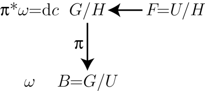
Figure 1: Fibration responsible for the presymplectic structure. $U\subseteq G$ is the subgroup that commutes with all Cartan generators $T_{i}$ with nonvanishing $e_{i}(0)$. The base manifold $B=G/U$is symplectic, which describes the type-B NGBs, while the fiber $F=U/H$ describes the type-A NGBs. The symplectic form $\omega$ on $B$ is pulled back to $\uppi^{*}\omega=\mathrm{d}c$ on $G/H$.

VII.2 Compact semisimple case

It is important to ask the following question: What kinds of coset spaces support a presymplectic structure? We have a definite answer to this question when $G$ is compact semisimple.

As we have seen, $c(\pi)=e_{i}(0)\omega^{i}$ is completely specified in terms of constants $e_{i}(0)$, where the generator $T_{i}$ commutes with the entire $H$ [see Eq. (92)]. Therefore, we can enlarge $H$ to include all generators that commute with $T_{i}$ to define the subgroup $U$ such that $U^{\dagger}e_{i}(0)T_{i}U=e_{i}(0)T_{i}$ in $G$. Mathematically, $e_{i}(0)T_{i}$ generates an Abelian group $T$, which is called a torus. Then, $U$ is called a centralizer of the torus $T$ in $G$. The following theorem proven by Borel Borel (1954) is then useful:

Let $G$ be compact semisimple and $U$ be the centralizer of a torus. Then, $G/U$ is homogeneous Kählerian and algebraic.

A torus $T$ in this context means an Abelian subgroup of $G$. Now, here is a new theorem of our own that follows from Eq. (94):

The presymplectic structure is determined uniquely with a Cartan element of the Lie algebra.

Namely, once $e_{i}(0)$ is specified, we know the symplectic structure. And, $e_{i}(0)$ generates a torus. For instance, an $\mathrm{SU}(N)$ group is simple and has many possible Abelian subgroups $T=\mathrm{U}(1),\mathrm{U}(1)^{2},\ldots\mathrm{U}(1)^{N-1}$. In general, a simple group admits a torus up to $T_{\text{max}}=\mathrm{U}(1)^{r}$, where $r$ is the rank of its Lie algebra, called the maximal torus $T_{\text{max}}$. An Abelian subgroup is called a torus because it is a manifold of coordinates with periodic boundary conditions for each, just like the surface of a doughnut (a two-torus). A centralizer $U$ of a torus $T$ is defined by the collection of elements in $G$ that commute with every element of $T$, i.e., $U=\{u\in G|utu^{-1}=t,\,\,\forall t\in T\}$. For instance, for

$$T=\{e^{i\,\mathrm{diag}(\overbrace{\alpha_{1},\ldots,\alpha_{1}}^{n_{1}},\,\overbrace{\alpha_{2},\ldots,\alpha_{2}}^{n_{2}},\,\cdots,\overbrace{\alpha_{k},\ldots,\alpha_{k}}^{n_{k}}\,)}\},$$

where $\sum_{i=1}^{k}n_{i}=N$ and $\sum_{i=1}^{k}n_{i}\alpha_{i}=0$ (traceless), $T=\mathrm{U}(1)^{k-1}\subset\mathrm{SU}(N)$, and its centralizer is $U=\mathrm{U}(1)^{k-1}\times\prod_{i=1}^{k}\mathrm{SU}(n_{i})$. Borel’s theorem then states then $G/U=\mathrm{SU}(N)/[\mathrm{U}(1)^{k-1}\times\prod_{i=1}^{k}\mathrm{SU}(n_{i})]$ is Kähler. A Kähler manifold always allows for a symplectic structure.

Therefore, this kind of a partially symplectic structure is possible on the coset space by considering the following fiber bundle $F\hookrightarrow G/H\stackrel{{\scriptstyle\uppi}}{{\rightarrow}}B$, where the base space $B=G/U$ is symplectic. (Note that we use the boldface $\uppi$ here to avoid a possible confusion with the NG field $\pi$.) The fiber is $F=U/H$. The symplectic structure $\omega$ on $B$ is pulled back by the projection $\uppi$ as $\uppi^{*}\omega$ on the entire coset space $G/H$. Since the closedness $\mathrm{d}\omega=0$ on $B$ implies the closedness $\mathrm{d}(\uppi^{*}\omega)=0$ on $G/H$, we can always find a one-form $c$ such that $\mathrm{d}c=\uppi^{*}\omega$ locally on $G/H$. Therefore, what we see in the Lagrangian at the first order in the time derivative is this pullback $\uppi^{*}\omega$ (further pulled back to spacetime by $\pi$).

The simplest example to see this structure is the $S^{3}=\text{U}(2)/\text{U}(1)$ as an $S^{1}$ fibration over $S^{2}$, as shown in Fig. 2. In this example, type-B NGBs live on the base space $S^{2}$, while the type-A NGB fluctuates along the $S^{1}$ fibers.

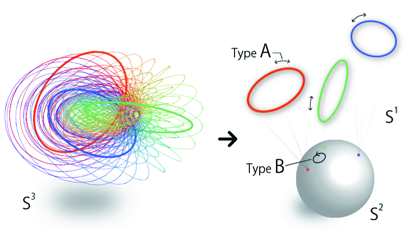
Figure 2: Graphical representation of the fibration $S^{1}\hookrightarrow S^{3}\stackrel{{\scriptstyle\uppi}}{{\rightarrow}}S^{2}$, where the projection $\uppi$ is the Hopf map. On each point on $S^{2}$, there is an $S^{1}$ fiber where the type-A NGB can fluctuate. The fiber on each point is shown with different colors. The type-B NGBs fluctuate on $S^{2}$. On the left, the entire $S^{3}$ is shown using a stereographic projection onto $\mathbb{R}^{3}$. $S^{1}$ Fibers are shown as circles, and the collection of circles form the entire $S^{3}$. Note that every circle is intertwined with every other circle.

The projection on a symplectic manifold makes sense from a physics point of view. In the long-distance limit, the modes with quadratic dispersion (typically, type-B) have much lower energies than those with linear dispersion (typically, type-A). Therefore, keeping only the type-B modes, namely, those with canonically-conjugate pairs, would make sense in this limit. It corresponds to the projection on the symplectic base manifold that describes type-B NGBs while eliminating the fiber that describes type-A NGBs.

The symplectic structure on $B=G/U$ is specified by parameters $e_{i}(0)$. Going back to the example of $G/U=\mathrm{SU}(N)/(\mathrm{U}(1)^{k-1}\times\prod_{i=1}^{k}\mathrm{SU}(n_{i}))$, using the exact sequence of the homotopy groups, it is seen that $\pi_{2}(G/U)=\pi_{1}(\mathrm{U}(1)^{k-1})/\pi_{1}(G)={\mathbb{Z}}^{k-1}$, while the Hurewicz theorem says that $H_{2}(G/U)=\pi_{2}(G/U)$ when $\pi_{1}(G/U)=0$. In addition, because $G/U$ is compact without a boundary, $H_{\text{dR}}^{2}=H_{2}(G/U,{\mathbb{R}})$ (de Rham theorem). Therefore, there are $k-1$ generators of $H^{2}_{\text{dR}}(G/U)$, $\omega_{1},\omega_{2},\ldots,\omega_{k-1}$, that can be used for the symplectic form $\omega=\sum_{i=1}^{k-1}a_{i}\omega_{i}$ on $G/U$. These numbers $a_{i}(i=1,\ldots,k-1)$ specify $\omega=dc$, and hence, $c=c_{a}d\pi^{a}$ in the Lagrangian. The number of $a_{i}$ is precisely the same number of parameters as $e_{i}(0)$ for this coset space.

In general, $\text{dim}\,H^{2}_{\text{dR}}(G/U)$ is the same as the number of $\text{U}(1)$ factors in $U$ when $G$ is semisimple [i.e., no $\text{U}(1)$ factors in $G$]. Pulled back to $G/H$, the possibilities of presymplectic structure correspond to the number $N_{\text{C}}$ of Cartan generators in $G$ that commute with $H$. We will use this fact extensively when we present the classification of possible presymplectic structures in the next section.

Note, however, that the linear combination $\omega=\sum_{i=1}^{k-1}a_{i}\omega_{i}$ may be degenerate for a certain choice of the parameters $a_{i}$. For instance, $G/H=\text{SU}(3)/\text{U}(1)\times\text{U}(1)$ is Kähler, has $H^{2}(G/H)={\mathbb{Z}}^{2}$, and supports a symplectic structure. There are two linearly independent closed invariant two-forms in Eq. (108): $\text{d}\omega^{3}$ [(109)] and $\text{d}\omega^{8}$ [(110)]. Note that $\omega^{3}$ and $\omega^{8}$ are not globally defined, as they transform inhomogeneously under the group transformations [see Eq. (76)]. Therefore, these two two-forms are closed but not exact, generate $H^{2}_{\text{dR}}[\text{SU}(3)/\text{U}(1)\times\text{U}(1)]$, and are candidates for the symplectic structure. Indeed, $\text{d}\omega^{3}=\text{d}\pi^{1}\wedge\text{d}\pi^{2}+(1/2)(\text{d}\pi^{4}\wedge\text{d}\pi^{5}-\text{d}\pi^{6}\wedge\text{d}\pi^{7})+O(\pi)^{3}$ and hence is nondegenerate. On the other hand, if we pick $\text{d}\omega^{8}=(\sqrt{3}/2)(\text{d}\pi^{4}\wedge\text{d}\pi^{5}+\text{d}\pi^{6}\wedge\text{d}\pi^{7})+O(\pi)^{3}$, it does not provide a canonical structure between $\pi^{1}$ and $\pi^{2}$, and hence, it is degenerate. There is actually a larger symmetry that preserves this choice because the torus is $\text{U}(1)$ generated by $T_{8}$ and its centralizer is $\text{U}(2)$. Then, it can be projected down to $\text{SU}(3)/\text{U}(2)=\mathbb{C}P^{2}$, where the fiber is $\text{U}(2)/\text{U}(1)\times\text{U}(1)=S^{2}$. This fibration is an example where the fiber is not a group .

VII.3 Case with central extensions

So far, we have assumed that $G$ is compact semisimple. If $G$ is not semisimple, especially if it has more than one $\text{U}(1)$ factor, its second cohomology $H^{2}(\mathfrak{g})$ is nontrivial and it allows for a central extension. See Appendix A for more discussions on the central extension.

In this case, $G/H$ may not necessarily be projected down to a symplectic manifold. Considering $G=\text{U}(1)^{3}$ and $H=\{e\}$, for an example, parametrized by three angles, $T^{3}=G/H=\{\varphi^{a}\in[0,2\pi)|a=1,2,3\}$ is a three-torus. We can introduce a presymplectic structure Chu (1974)

$$\omega=\mathrm{d}\varphi^{1}\wedge(\mathrm{d}\varphi^{2}+r\mathrm{d}\varphi^{3}).$$ (224)

If $r$ is a rational number $r=p/q$ for $p$ and $q$ relatively prime, the orbit winds around $T^{3}$ $q$ times and closes on itself. Then, there is a well-defined projection down to $T^{2}$. On the other hand, if $r$ is an irrational number, there is no well-defined projection because the orbit winds around $T^{3}$ infinite times without closing on itself.

We suspect that such a pathological case would not arise in physical systems. Yet, we do not have a concrete proof of what goes wrong in such a case.

VII.4 Quantization condition

The normalization of the presymplectic structure may be quantized. All discussions above are, so far, concerned with the invariance of the action up to a surface term. In classical physics, the action itself does not have a physical meaning while its variation leads to the equations of motion. In quantum physics, however, the action itself goes into the path integrals as $e^{iS/\hbar}$, and hence, its value matters. Yet, a change in the action by integer multiples of $2\pi\hbar$ does not change the path integral. Recall that we use the unit $\hbar=1$ in this paper, and henceforth, we drop $\hbar$ in expressions.

When $\omega=\text{d}c$ is closed but not exact, namely, an element of $H^{2}_{\text{dR}}(G/H)$, its coefficient is quantized. Considering a time integral to be a periodic loop $L^{1}$ on $G/H$, the loop can be viewed as a boundary of a two-disk. [Here, we assume $\pi_{1}(G/H)=0$, so that every loop on $G/H$ is contractible to a point.] However, nontrivial $H^{2}_{\text{dR}}$ implies nontrivial $H_{2}$, and hence, there are noncontractible two-cycles on $G/H$. Namely, there are nontrivial closed two-dimensional surfaces $C_{2}$ in $G/H$. Then, $C_{2}=C_{2}^{+}\cup C_{2}^{-}$ is a union of two surfaces that share the same boundary $L^{1}=\partial C_{2}^{+}=-\partial C_{2}^{-}$. The simplest example is $C_{2}\simeq S^{2}$, where $L^{1}$ is the equator, $C_{2}^{+}$ the northern hemisphere, and $C_{2}^{-}$ the southern hemisphere. For the action

$$S\ni\int\text{d}^{d}x\int_{L_{1}}c$$ (225)

to give a single valued $e^{iS}$, its ambiguity

$$\Delta S=\int\mathrm{d}^{d}x\int_{C_{2}^{+}}\mathrm{d}c-\int\mathrm{d}^{d}x\int_{-C_{2}^{-}}\mathrm{d}c=\int\mathrm{d}^{d}x\int_{C_{2}}\mathrm{d}c$$ (226)

must be quantized in units of $2\pi$. This discussion is the same as the one on Wess-Zumino-Witten terms in Sec. III.5.3.

When the system is finite $\Omega=\int\mathrm{d}^{d}x<\infty$, the quantization condition restricts the normalization of $c$. In other words, $\Omega\mathrm{d}c$ is an element of $H^{2}(G/H,{\mathbb{Z}})$ rather than $H^{2}_{\text{dR}}(G/H)=H^{2}(G/H,{\mathbb{R}})$.

The same consideration applies to central extensions. When the target space is compact, the (pre)symplectic form is quantized. For example, for $\text{U}(1)^{2}=\{(\varphi^{1},\varphi^{2})|\varphi^{i}\in[0,2\pi)\}$, $\Omega\mathrm{d}c=k(2\pi)^{-1}\mathrm{d}\varphi^{1}\wedge\mathrm{d}\varphi^{2}$ with $k\in{\mathbb{Z}}$. On the other hand, when the target space is non-compact, such as ${\mathbb{R}}^{2}={\mathbb{C}}$ in the case of the free Schrödinger field mentioned in Sec. III.5 and Appendix C, the coefficient is not quantized.

VIII Classification of Possible Presymplectic Structures

As we have seen in Sec. VII, a presymplectic structure on a coset space $G/H$ is characterized by its fibration on a symplectic base space $B=G/U$ with the fiber $F=U/H$, when $G$ and $H$ are compact semisimple. $U\subset G$ is the subgroup that commutes with generators with nonzero $e_{i}(0)$. Since $e_{i}(0)$’s need to be invariant under $H$ [Eq. (92)], $H\subset U$. The base space describes type-B NGBs while the fiber describes type-A NGBs. In this section, we show how such structures can be completely classified.

VIII.1 Preliminary discussions

The number of type-A and type-B NGBs is given by the counting rule in Eqs. (1) and (2). If the rank of $\rho$ explores all the possible integral values in the range

$$0\leq\text{rank}\rho\leq\text{dim}\,G/H,$$ (227)

the number of type-A and type-B NGBs can be any combinations between $(n_{\text{A}},n_{\text{B}})=(\text{dim}\,G/H,0)$ and $(0,\frac{1}{2}\text{dim}\,G/H)$. Indeed, in the case of Heisenberg magnets $G/H=\text{SO}(3)/\text{SO}(2)$ ($\text{dim}\,G/H=2$), antiferromagnets and ferromagnets, respectively, realize the case $\text{rank}\rho=0,1$. However, in this section, we discuss that, in general, allowed values of $\text{rank}\rho$ are strongly constrained.

In general, we can always choose the basis of generators in such a way that only Cartan generators Georgi (1999) of $G$ that commute with all generators of $H$ may have a nonzero expectation value $\langle j_{i}^{0}(\vec{x},t)\rangle\neq 0$ Watanabe and Brauner (2011), as we have discussed in previous sections. Their expectation values specify $e_{i}(0)$, and the corresponding generators generate the torus $T$. Each nonzero expectation value of conserved charge densities defines a presymplectic structure on $G/H$ by $c=-e_{i}(0)\omega^{i}$ [Eq. (94)]; namely, it makes NG fields associated with broken generators $Q_{a}$ and $Q_{b}$ canonically conjugate to each other, as discussed in Sec. VII

For a given $G$ and $H$, let $N_{\text{C}}$ be the number of Cartan generators of $\mathfrak{g}$ that commute with $\mathfrak{h}$. Based on the above considerations, we know that these generators are the only ones that are allowed to have nonvanishing $e_{i}(0)$. Therefore, there are $N_{\text{C}}$ parameters to specify the possible presymplectic structure on $G/H$. This counting takes into account only the connected component $G_{0}$ of the identity, and the discrete subgroup $G/G_{0}$ might further restrict allowed presymplectic structures.

Therefore, we first consider the case when $H$ is generated by Cartan generators alone, so that all Cartan generators commute with $\mathfrak{h}$ to maximize $N_{\text{C}}$.

VIII.2 Flag manifolds

To study the case of maximum $N_{\text{C}}$ for a given $G$, let us consider the flag manifolds $G/\text{U}(1)^{r}$, where $N_{\text{C}}=r\geq 1$ is the rank of the simple group $G$. We can systematically enumerate all possibilities of presymplectic structures for them. It turns out that this list allows us to also classify possibilities for other $G/H$ as well. In this sense, the discussion here is the basis of all other cases. For concreteness, we first discuss $\text{SU}(n+1)/\text{U}(1)^{n}$.

A flag manifold is Kähler, thanks to the Borel theorem Borel (1954), and is hence symplectic. Indeed, for $\text{SU}(n+1)/\text{U}(1)^{n}$, $\text{dim}\,{G/H}=n(n+1)$ is always even. Since all Cartan generators of $G$ remain unbroken, $N_{\text{C}}=n$ and there are many presymplectic structures that can control the number of type-A and type-B NGBs. The simplest case of $\text{SU}(3)/\text{U}(1)^{2}$ with $N_{\text{C}}=2$ is shown in Table 2.

The two limiting cases can easily be understood. Any symplectic manifold is endowed with an associated symplectic two-form, which always realizes the case $\mathrm{rank}\rho=\text{dim}\,{G/H}$. (Unless discrete the subgroup puts out an obstacle.) Thus, we know that $(n_{\text{A}},n_{\text{B}})=(0,n(n+1)/2)$ is possible. Also, by setting all expectation values of charge densities to be $0$, one can realize the case where $\mathrm{rank}\rho=0$, and hence, $(n_{\text{A}},n_{\text{B}})=(n(n+1),0)$.

The question is whether it is possible to realize combinations of $(n_{\text{A}},n_{\text{B}})$ between these two limiting cases. Although there are $N_{\text{C}}=n$ parameters to control, the number of integers in the range Eq. (227) grows as $n^{2}$, so obviously, it is not possible to realize all of these values for a large $n$. For example, there is a minimum value of $\mathrm{rank}\,\rho$ (except for $0$), which is achieved by the presymplectic structure that appeared in the above discussion of $\text{SU}(n+1)/\text{U}(n)=\mathbb{C}P^{n}$ model. This presymplectic structure gives $\mathrm{rank}\rho=n$, and $0<\mathrm{rank}\rho<n$ is prohibited.

Table 2: Possible number of type-A and type-B NGBs for $\text{SU}(3)/\text{U}(1)\times\text{U}(1)$.

$n_{\text{A}}$	$n_{\text{B}}$	$F=U/H$	$B=G/U$
6	0	$\text{SU}(3)/\text{U}(1)\times\text{U}(1)$	$\{e\}$
2	2	$\text{SU}(2)/\text{U}(1)$	$\text{SU}(3)/\text{SU}(2)\times\text{U}(1)$
0	3	$\{e\}$	$\text{SU}(3)/\text{U}(1)\times\text{U}(1)$

The case for simple classical groups is straightforward to work out. The smallest possible $H$ that makes $G/H$ symplectic is the flag manifold $H=\text{U}(1)^{r}$, where $r$ is the rank of $G$. All Cartan generators commute with $\text{U}(1)^{r}$, and hence, $N_{\text{C}}=r$. Therefore, this case allows for the largest number of possible choices for $U$.

Because $e_{i}(0)$ belong to the adjoint representation, the corresponding generators $T_{i}$ generate a torus $T$, and its centralizer $U$ is generated by all generators of $\mathfrak{g}$ that leave $e_{i}(0)$ invariant. Such symmetry-breaking patterns have been studied extensively in the literature (see, e.g., Ref. Intriligator et al. (1995)).

For $\text{SU}(n)$ groups, the possible form of $e_{i}(0)T_{i}$ is

$$e_{i}(0)T_{i}=\mathrm{diag}(\overbrace{\alpha_{1},\ldots,\alpha_{1}}^{n_{1}},\,\overbrace{\alpha_{2},\ldots,\alpha_{2}}^{n_{2}},\,\ldots,\overbrace{\alpha_{k},\ldots,\alpha_{k}}^{n_{k}}\,),$$ (228)

and the corresponding centralizer is

$$U=\text{U}(1)^{k-1}\times\prod_{k}\text{SU}(n_{k}),\quad n=\sum_{k}n_{k},\quad\sum_{k}n_{k}\alpha_{k}=0.$$ (229)

In this expression, $\text{SU}(1)$ counts as a trivial group.

For $\text{SO}(n)$ groups, any element of the adjoint representation is an antisymmetric matrix that can be skew diagonalized. Therefore, the possible form of $e_{i}(0)T_{i}$ is

$$e_{i}(0)T_{i}=\mathrm{diag}(\overbrace{0,\ldots,0}^{m},\,\overbrace{\alpha_{1},\ldots,\alpha_{1}}^{n_{1}},\,\ldots,\overbrace{\alpha_{k},\ldots,\alpha_{k}}^{n_{k}}\,)\otimes i\sigma_{2},$$ (230)

and we find the centralizer

$$U=\text{SO}(m)\times\prod_{k}\text{U}(n_{k}),\qquad n=m+2\sum_{k}n_{k}.$$ (231)

Finally, for $\text{Sp}(n)$ groups [we use the notation that the rank is $n$ for $\text{Sp}(n)$], every element $g\in\text{Sp}(n)$ preserves

$$J=\left(\begin{array}[]{c|c}0&-I_{n}\\ \hline\cr I_{n}&0\end{array}\right),\qquad gJg^{T}=J.$$ (232)

Therefore, the adjoint representation is a $2n\times 2n$ matrix of the form

$$S=\left(\begin{array}[]{c|c}A&B\\ \hline\cr C&-A^{T}\end{array}\right),\qquad SJ+JS^{T}=0.$$ (233)

Here, $B^{T}=B$ and $C^{T}=C$ are symmetric matrices. The Cartan generators are given by the diagonal matrices in $A$ with $B=C=0$ and therefore have the form $S=A_{\text{diag}}\otimes\sigma_{3}$. In general,

$$e_{i}(0)T_{i}=\mathrm{diag}(\overbrace{0,\ldots,0}^{m},\,\overbrace{\alpha_{1},\ldots,\alpha_{1}}^{n_{1}},\,\ldots,\overbrace{\alpha_{k},\ldots,\alpha_{k}}^{n_{k}}\,)\otimes\sigma_{3},$$ (234)

and we find

$$U=\text{Sp}(m)\times\prod_{k}\text{U}(n_{k}),\qquad n=m+\sum_{k}n_{k}.$$ (235)

The problem is basically listing up a partition of integers.

Once all possibilities $U$ are listed, it is easy to count $n_{\text{A}}=\text{dim}\,U/H$ and $n_{\text{B}}=\text{dim}\,G/U$. We present all possible cases for rank-five groups in tables: $\text{SU}(6)$ (Table 3), $\text{SO}(10)$ (Table 4), and $\text{SO}(11)$ and $\text{Sp}(5)$ (Table 5).

Looking at Table 4, one might think that $U=\text{SO}(6)\times\text{U}(1)^{2}$ and $U=\text{U}(4)\times\text{U}(1)$ are the same because $\mathfrak{so}(6)$ and $\mathfrak{su}(4)$ are identical Lie algebras. They are not. The spectrum of the 14 type-B NGBs on $\text{SO}(10)/[\text{SO}(6)\times\text{U}(1)^{2}]=\text{SO}(10)/[\text{SU}(4)/\mathbb{Z}_{2}\times\text{U}(1)^{2}]$ consists of $14=6+6+1+1$ under $\text{SO}(6)$, while those on $\text{SO}(10)/(\text{U}(4)\times\text{U}(1))=\text{SO}(10)/\{[\text{SU}(4)\times\text{U}(1)]/{\mathbb{Z}}_{4}\times\text{U}(1)\}$ consist of $14=4+4+6$ under $\text{SU}(4)$. The same comment applies to $\text{SO}(4)\times\text{U}(1)^{3}$ vs $\text{U}(2)^{2}\times\text{U}(1)$ as $\mathfrak{so}(4)=\mathfrak{su}(2)\oplus\mathfrak{su}(2)$. On $\text{SO(10)}/[\text{SO}(4)\times\text{U}(1)^{3}]$, the type-B spectrum is $18=4\times 3+1\times 6$ under $\text{SO}(4)$, while for $\text{SO}(10)/[\text{U}(2)^{2}\times\text{U}(1)]$, it is $18=(2,2)\times 2+(2,1)\times 2+(1,2)\times 2+(1,1)\times 2$ under $\text{U}(2)\times\text{U}(2)$. Therefore, one has to be careful about not identifying local isomorphisms among groups.

On the other hand, in the case of $\text{SO}(n)$ with $n$ even, it can break to $U=\text{SO}(2)\times\prod_{k}\text{U}(n_{k})$. Turning $e_{i}(0)$ for the $\text{SO}(2)$ generator would “break” it further to $\text{U}(1)$ with no difference in the group structure or representations of NGBs. Namely, two cases are continuously connected without an order parameter that distinguishes them. Therefore, we can identify $\text{SO}(2)$ and $\text{U}(1)$ and we have eliminated duplicates from Table 4.

Note that there is a duality between $\text{Sp}(n)$ and $\text{SO}(2n+1)$ groups in each symmetry-breaking pattern because the dimensions of the group match: $(1/2)(2n+1)2n=n(2n+1)$ for $\text{SO}(2n+1)$, and $(1/2)2n(2n+1)=n(2n+1)$ for $\text{Sp}(n)$.

Table 3: Possible number of type-A and type-B NGBs for $\text{SU}(6)/\text{U}(1)^{5}$.

$n_{\text{A}}$	$n_{\text{B}}$	$U$
30	0	$\{e\}$
20	5	$\text{SU}(5)\times\text{U}(1)$
14	8	$\text{SU}(4)\times\text{SU}(2)\times\text{U}(1)$
12	9	$\text{SU}(4)\times\text{U}(1)^{2}$
12	9	$\text{SU}(3)^{2}\times\text{U}(1)$
8	11	$\text{SU}(3)\times\text{SU}(2)\times\text{U}(1)^{2}$
6	12	$\text{SU}(3)\times\text{U}(1)^{3}$
6	12	$\text{SU}(2)^{3}\times\text{U}(1)^{2}$
4	13	$\text{SU}(2)^{2}\times\text{U}(1)^{3}$
2	14	$\text{SU}(2)\times\text{U}(1)^{4}$
0	15	$\text{U}(1)^{5}$

Table 4: Possible number of type-A and type-B NGBs for $\text{SO}(10)/\text{U}(1)^{5}$.

$n_{\text{A}}$	$n_{\text{B}}$	$U$
40	0	$\{e\}$
24	8	$\text{SO}(8)\times\text{U}(1)$
20	10	$\text{U}(5)$
14	13	$\text{SO}(6)\times\text{U}(2)$
12	14	$\text{SO}(6)\times\text{U}(1)^{2}$
12	14	$\text{U}(4)\times\text{U}(1)$
10	15	$\text{SO}(4)\times\text{U}(3)$
8	16	$\text{U}(3)\times\text{U}(2)$
6	17	$\text{SO}(4)\times\text{U}(2)\times\text{U}(1)$
6	17	$\text{U}(3)\times\text{U}(1)^{2}$
4	18	$\text{SO}(4)\times\text{U}(1)^{3}$
4	18	$\text{U}(2)^{2}\times\text{U}(1)$
2	19	$\text{U}(2)\times\text{U}(1)^{3}$
0	30	$\text{U}(1)^{5}$

Table 5: Possible number of type-A and type-B NGBs for $\text{SO}(11)/\text{U}(1)^{5}$ and $\text{Sp}(5)/\text{U}(1)^{5}$.

$n_{\text{A}}$	$n_{\text{B}}$	$U\subset\text{SO}(11)$	$U\subset\text{Sp}(5)$
50	0	$\{e\}$	$\{e\}$
32	9	$\text{SO}(9)\times\text{U}(1)$	$\text{Sp}(4)\times\text{U}(1)$
20	15	$\text{SO}(7)\times\text{U}(2)$	$\text{Sp}(3)\times\text{U}(2)$
20	15	$\text{U}(5)$	$\text{U}(5)$
18	16	$\text{SO}(7)\times\text{U}(1)^{2}$	$\text{Sp}(3)\times\text{U}(1)^{2}$
14	18	$\text{SO}(5)\times\text{U}(3)$	$\text{Sp}(2)\times\text{U}(3)$
14	18	$\text{SO}(3)\times\text{U}(4)$	$\text{Sp}(1)\times\text{U}(4)$
12	19	$\text{U}(4)\times\text{U}(1)$	$\text{U}(4)\times\text{U}(1)$
10	20	$\text{SO}(5)\times\text{U}(2)\times\text{U}(1)$	$\text{Sp}(2)\times\text{U}(2)\times\text{U}(1)$
8	21	$\text{SO}(5)\times\text{U}(1)^{3}$	$\text{Sp}(2)\times\text{U}(1)^{3}$
8	21	$\text{SO}(3)\times\text{U}(3)\times\text{U}(1)$	$\text{Sp}(1)\times\text{U}(3)\times\text{U}(1)$
8	21	$\text{U}(3)\times\text{U}(2)$	$\text{U}(3)\times\text{U}(2)$
6	22	$\text{SO}(3)\times\text{U}(2)^{2}$	$\text{Sp}(1)\times\text{U}(2)^{2}$
6	22	$\text{U}(3)\times\text{U}(1)^{2}$	$\text{U}(3)\times\text{U}(1)^{2}$
4	23	$\text{SO}(3)\times\text{U}(2)\times\text{U}(1)^{2}$	$\text{Sp}(1)\times\text{U}(2)\times\text{U}(1)^{2}$
4	23	$\text{U}(2)^{2}\times\text{U}(1)$	$\text{U}(2)^{2}\times\text{U}(1)$
2	24	$\text{SO}(3)\times\text{U}(1)^{4}$	$\text{Sp}(1)\times\text{U}(1)^{4}$
2	24	$\text{U}(2)\times\text{U}(1)^{3}$	$\text{U}(2)\times\text{U}(1)^{3}$
0	25	$\text{U}(1)^{5}$	$\text{U}(1)^{5}$

It should be possible to enumerate possibilities for exceptional groups $G_{2}$, $F_{4}$, and $E_{6,7,8}$ as well, but we do not attempt it here.

VIII.3 General $H$

For more general $G/H$, we start with the list of possible $U$ for $G/\text{U}(1)^{r}$ and remove those that do not commute with $H$. It gives all possible presymplectic structures. The number of type-B NGBs is given by $n_{\text{B}}=(1/2)\text{dim}\,G/U$, while $n_{\text{A}}={\rm dim}U/H$. Let us discuss a few examples below.

For instance, one can consider $\text{SU}(6)/\text{SU}(5)$, whose dimension is $35-24=11$. Note that $\text{SU}(6)/\text{SU}(5)=\text{U}(6)/\text{U}(5)=S^{11}$ which is discussed in Sec. IX.3. Looking at the list in Table 3, the only $U$ that commutes with $\text{SU}(5)$ is in the top two. Therefore, there are two types of presymplectic structures possible on $\text{SU}(6)/\text{SU}(5)$. If $U$ is trivial, all 11 are type-A NGBs. If $U=\text{SU}(5)\times\text{U}(1)$, $B=\text{SU}(6)/[\text{SU}(5)\times\text{U}(1)]={\mathbb{C}}\text{P}^{5}$ and there are five type-B NGBs for $(1/2){\rm dim}B=5$. There is only one type-A NGB.

If the same $\text{SU}(6)$ is broken by an order parameter in a rank-three antisymmetric tensor, the unbroken group is $H=\text{SU}(3)\times\text{SU}(3)$. In this case, there is no $U$ that commutes with $H$ except for the trivial one. Namely, this coset space allows for no presymplectic structure, and hence, $n_{\text{A}}=19$ and $n_{\text{B}}=0$. However, if one of the $\text{SU}(3)$ is further broken completely by order parameters in fundamental representations (at least two of them), $H=\text{SU}(3)$ commutes with the first seven choices of $U$ in Table 3, and there are accordingly seven possibilities of $(n_{\text{A}},n_{\text{B}})$.

This way, one can work out all possibilities of $(n_{\text{A}},n_{\text{B}})$ for a given $G$ and $H$ if compact and simple. Then, we look at discrete subgroups if $G$ or $H$ has more than one connected component to further eliminate some possibilities. It is also straightforward to study examples with additional $\text{U}(1)$ factors, paying attention to possible central extensions.

This way, one can enumerate all possible presymplectic structures for a given $G/H$ and write down the most general effective Lagrangians using the explicit forms we found in Sec. III.

IX Examples

Having developed a complete classification of presymplectic structures, we revisit popular examples of coset spaces in the literature and show what effective Lagrangians are possible for them.

IX.1 $\text{O}(n+1)/\text{O}(n)=S^{n}$

For $\text{O}(n+1)/\text{O}(n)=S^{n}$, $\text{SO}(n+1)/\text{SO}(n)=S^{n}$, and $\text{O}(n+1)/[\text{O}(n)\times\mathbb{Z}_{2}]=\mathbb{R}P^{n}$, there is no possible presymplectic structure for $n\geq 3$. As seen in Tables 4 and 5, there is no nontrivial $U$ that commutes with the $\text{SO}(n)$ subgroup within $\text{SO}(n+1)$, and hence, $N_{\text{C}}=0$. Therefore, we can only have $n$ type-A NGBs. The most general Lagrangian is hence

$$\mathcal{L}_{\text{eff}}=\frac{1}{2}\bar{g}_{0}\dot{n}_{i}\dot{n}_{i}-\frac{1}{2}g_{0}\vec{\nabla}n_{i}\cdot\vec{\nabla}n_{i}$$ (236)

up to the second order in derivatives, where $\vec{n}$ is a normalized $(n+1)$-component vector.

When $n=2$, all of these examples have $N_{\text{C}}=1$ and the coset $\text{SO}(3)/\text{SO}(2)=S^{2}$ indeed describes both ferro- and antiferromagnets. However, for $\text{O}(3)/\text{O}(2)=S^{2}$, there is no presymplectic structure that is consistent with the discrete subgroup $\{+\openone,-\openone\}$, at least when we realize it as an internal symmetry. To see this point, let us parametrize the coset $S^{2}$ by the spherical coordinate $(\theta,\phi)$. The candidate of a one-form that is associated with the would-be symplectic structure is $\cos\theta\dot{\phi}$, but it changes sign under $-\openone$: $\theta\rightarrow\pi-\theta$ and $\phi\rightarrow\phi+\pi$ unless the discrete symmetry incorporates with the time reversal $t\rightarrow-t$. The coset $\text{O}(3)/[\text{O}(2)\times\mathbb{Z}_{2}]=\mathbb{R}P^{2}$ can be discussed in a similar fashion, but since $\mathbb{R}P^{2}$ is not even orientable, there is obviously no symplectic structure that is consistent with the global topology of $G/H$.

IX.2 $\text{SU}(n+1)/\text{U}(n)=\mathbb{C}P^{n}$

The $\mathbb{C}P^{n}$ ($n\geq 1$) model is a natural generalization of ferromagnets based on $S^{2}=\mathbb{C}P^{1}$. For $G/H=\text{SU}(n+1)/\text{U}(n)=\mathbb{C}P^{n}$, $N_{\text{C}}=1$ because there is a unique Cartan generator $\text{diag}(n,-1,\ldots,-1)$ that commutes with $H=\text{U}(n)$. Therefore, there is a unique symplectic structure on $G/H$ (up to an overall normalization). The effective Lagrangian can be most conveniently expressed in terms of an $n$-component complex field $z(\vec{x},t)\in\mathbb{C}^{n}$, and the most general effective Lagrangian to the quadratic order in derivatives is given by

$$\mathcal{L}_{\text{eff}}=is_{0}\frac{z^{\dagger}\dot{z}-\dot{z}^{\dagger}z}{1+z^{\dagger}z}+G_{ab}\left(\bar{g}_{0}\dot{\bar{z}}^{a}\dot{z}^{b}-g_{0}\vec{\nabla}\bar{z}^{a}\cdot\vec{\nabla}z^{b}\right),$$ (237)

where

$$G_{ab}(\bar{z},z)=\frac{\delta_{ab}(1+\bar{z}z)-\bar{z}^{b}z^{a}}{(1+\bar{z}z)^{2}}$$ (238)

is the Fubini-Study metric on $\mathbb{C}P^{n}$ Nakahara (2003); Eguchi et al. (1980). In $2+1$ dimensions, we can add a topological term ($\theta$-term) $(i/2\pi)G_{ab}(\bar{z},z)\epsilon^{ij}\partial_{i}\bar{z}^{a}\partial_{j}z^{b}$. The $n=1$ case is identical to ferromagnets (recall that $\mathbb{C}P^{1}=S^{2}$). The coefficient of the first term $s_{0}$ is the charge density of the ground state $\langle j_{\rho_{0}}^{0}(x)\rangle$, where $\rho_{0}$ is the U(1) part of the unbroken subgroup $H=\text{U}(n)$. This term $s_{0}\Omega$ must be quantized to a half-integer, where $\Omega$ is the volume of the system, as discussed in Sec. VII.4. When $s_{0}\neq 0$, the system resembles ferromagnets: The real and imaginary parts of $z^{a}$ become canonically conjugate to each other, and there are $n$ type-B NGBs. On the other hand, when $s_{0}=0$, the ground state is antiferromagnetic and there are $2n$ type-A NGBs. Other possibilities $(n_{\text{A}},n_{\text{B}})=(2,n-1),(4,n-2),\ldots,(2n-2,1)$ cannot be realized.

IX.3 $\text{U}(n+1)/\text{U}(n)=S^{2n+1}$

$\text{U}(n+1)/\text{U}(n)=S^{2n+1}$ ($n\geq 1$) is topologically the same as $\text{SO}(2n+2)/\text{SO}(2n+1)$, yet its field theory is very different because $N_{\text{C}}=1$ for the generator $\text{diag}(n,-1,\ldots,-1)$. It is closely related to the $\mathbb{C}P^{n}$ model since it admits a fibration $S^{1}\hookrightarrow S^{2n+1}\stackrel{{\scriptstyle\uppi}}{{\rightarrow}}\mathbb{C}P^{n}$, where type-B NGBs live on the base manifold $\mathbb{C}P^{n}$ and a type-A NGB is in the fiber $S^{1}$. Therefore, there are only two possibilities $(n_{\text{A}},n_{\text{B}})=(1,n)$ and $(2n+1,0)$, which is expected from $N_{\text{C}}=1$. The case $n=1$ of this model describes the physics of Kaon condensation Miransky and Shovkovy (2002); Schäfer et al. (2001). The generalization to $n\geq 1$ is discussed in Ref. Andersen .

As a concrete example, let us consider a $\mathrm{U}(n+1)$-symmetric Schrödinger field

$$\mathcal{L}=i\psi^{\dagger}\dot{\psi}-\frac{1}{2m}\vec{\nabla}\psi^{\dagger}\cdot\vec{\nabla}\psi-\frac{\lambda}{2}(\psi^{\dagger}\psi-n_{0})^{2},$$ (239)

where $\psi(x)$ is a complex $(n+1)$-dimensional column vector. A similar model was discussed in Refs. Miransky and Shovkovy (2002); Schäfer et al. (2001). At the tree level, it has the vacuum

$$\langle\psi\rangle=\sqrt{n_{0}}(1,0,\ldots,0)^{T}.$$ (240)

In this case, the original $\mathrm{U}(n+1)$ symmetry is broken to $\mathrm{U}(n)$ symmetry. The coset space $\mathrm{U}(n+1)/\mathrm{U}(n)=S^{2n+1}$ does not admit a symplectic structure.

Therefore, we have to carefully parametrize the coset space. Since $\mathrm{U}(n+1)/[\mathrm{U}(n)\times\mathrm{U}(1)]\cong\mathbb{C}P^{n}$, which does admit a symplectic structure, we view $S^{2n+1}$ as a $\mathrm{U}(1)$ bundle on $\mathbb{C}P^{n}$. The symplectic two-form lives on $\mathbb{C}P^{n}$. We parametrize the field $\psi(x)$ as

$$\psi=\sqrt{n}\frac{e^{-i\theta}}{\sqrt{1+z^{\dagger}z}}\begin{pmatrix}1\\ z\end{pmatrix},$$ (241)

where $z(x)$ is an $n$-dimensional column vector. Substituting the above parametrization, we find

$$\mathcal{L}_{\text{eff}} = n_{0}\left(\dot{\theta}+\frac{i}{2}\frac{z^{\dagger}\dot{z}-\dot{z}^{\dagger}z}{1+z^{\dagger}z}\right)-\frac{1}{2\lambda}\left(\dot{\theta}+\frac{i}{2}\frac{z^{\dagger}\dot{z}-\dot{z}^{\dagger}z}{1+z^{\dagger}z}\right)^{2}$$ (242)

$$-\frac{n_{0}}{2m}\left(\vec{\nabla}\theta+\frac{i}{2}\frac{z^{\dagger}\vec{\nabla}z-\vec{\nabla}z^{\dagger}z}{1+z^{\dagger}z}\right)^{2}$$

$$-\frac{n_{0}}{2m}\left(\frac{\vec{\nabla}z^{\dagger}\vec{\nabla}z}{1+z^{\dagger}z}-\frac{(\vec{\nabla}z^{\dagger}z)(z^{\dagger}\vec{\nabla}z)}{(1+z^{\dagger}z)^{2}}\right)+\cdots.$$

The second term arises from integrating out $n$ at the tree level and looks the same as the terms $O(\vec{\nabla}^{2})$, except for the overall normalization because of the irreducible nature of $\theta$ and $z^{i}$ under $H=\text{U}(n)$.

The terms in the last parentheses above are nothing but the Fubini-Study metric on $\mathbb{C}P^{n}$, which is Kähler. On the other hand, the first term defines a one-form

$$c=i\frac{z^{\dagger}\mathrm{d}z-\mathrm{d}z^{\dagger}z}{1+z^{\dagger}z},$$ (243)

while its exterior derivative

$$\mathrm{d}c=i\frac{(1+z^{\dagger}z)\mathrm{d}z^{\dagger}\wedge\mathrm{d}z-(\mathrm{d}z^{\dagger}z)\wedge(z^{\dagger}\mathrm{d}z)}{(1+z^{\dagger}z)^{2}}$$ (244)

is the Kähler form on $\mathbb{C}P^{n}$ associated with the Fubini-Study metric. The coordinate $\theta$ represents the U(1), which is orthogonal to the tangent vectors of $\mathbb{C}P^{n}$.

In Sec. X, we derive the effective Lagrangian for $n=1$ based purely on the Galilean symmetry and the $\text{U}(2)$ internal symmetry. We should be able to rewrite the Lagrangian (242) in terms of the Galilean-covariant derivatives,

$$\mathscr{D}_{t}\theta=\dot{\theta}-\frac{(\vec{\nabla}\theta)^{2}}{2m},$$ (245)

$$\mathscr{D}_{t}z=\dot{z}-\frac{\vec{\nabla}\theta\cdot\vec{\nabla}z}{m},\quad\vec{\mathscr{D}}z=\vec{\nabla}z,$$ (246)

neglecting higher-order derivatives. Comparing Eq. (239) with Eq. (291), we notice that the Lagrangian lacks the term that contains $\mathscr{D}_{t}z^{\dagger}\mathscr{D}_{t}z$. In general, if we start from a particular microscopic model and work only at tree levels, the effective Lagrangian may not include all possible terms allowed by symmetries. Missing terms are often generated by higher corrections .

X Galilean invariance

So far, our discussions have focused on the spontaneous breaking of internal symmetries. However, in many interesting physical systems, spacetime symmetries are also spontaneously broken. For the sake of the clarity of our discussions, we restrict ourselves to translationally and rotationally invariant systems in this paper. Therefore, we discuss spontaneously broken Galilean invariance as an illustrative example in this section. We demonstrate how spacetime symmetries can be discussed within our effective Lagrangian formalism and see how they provide additional constraints on the parameters in the theory. The so-called inverse Higgs mechanism provides a heuristic method to show how would-be NGB degrees of freedom can be consistently removed from the physical spectrum in accordance with observations. This method was discussed mostly in Lorentz-invariant systems, and our presentation here shows how it can be successfully extended to Lorentz-noninvariant systems.

It has recently been argued Son and Wingate (2006) that some classes of Galilean-invariant theories can be promoted to be nonrelativistic general-coordinate invariant, by introducing the spatial metric $g_{ij}(\vec{x},t)$ and the $\text{U}(1)$ gauge field and by assigning their nontrivial transformation rule. The Galilean symmetry itself is global in the sense that the velocity parameter in $\vec{x}^{\prime}=\vec{x}+\vec{v}t$ is a constant, but the nonrelativistic general-coordinate invariance allows a more general local transformation $\vec{x}^{\prime}(\vec{x},t)$ with arbitrary time dependence (but still, $t^{\prime}=t$). Such an extended symmetry strongly restricts the response of the system to external fields. Our discussion below should be useful to systematically produce general-coordinate-invariant combinations.

X.1 Coset construction with spacetime symmetries

In condensed-matter physics, superfluid helium and various types of Bose-Einstein condensates often spontaneously break the Galilean symmetry as well as the U(1) phase rotation. In such a situation, one has to make sure that the effective Lagrangian has the Galilean symmetry.

Here, we discuss how to incorporate spacetime symmetries in our effective Lagrangian. Spacetime symmetries are those which change coordinates $x^{\mu}=(t,\vec{x})$ in addition to the fields. For example, the transformation rule of the superfluid phase under the Galilean transformation is

$$\vec{x}^{\prime} = \vec{x}+\vec{v}_{0}t,\quad t^{\prime}=t,$$ (247)

$$\theta^{\prime}(\vec{x}^{\prime},t^{\prime}) = \theta(\vec{x},t)-m\vec{v}_{0}\cdot\vec{x}-\frac{mv_{0}^{2}}{2}t,$$ (248)

for a constant vector $\vec{v}_{0}\in\mathbb{R}^{3}$. Since $\vec{x}$ changes, Galilean symmetry is a spacetime symmetry.

For simplicity, here, we discuss the situation where the spacetime translation $P_{\mu}=(H,-\vec{P})$ is not broken, and unbroken generators $Q_{\rho}$ are internal symmetries, while broken generators $Q_{a}$ may contain spacetime symmetries such as the Galilean boost generator.

Following Ref. Ivanov and Ogievetsky (1975), we use

$$U(x,\pi(x))=e^{ix^{\mu}P_{\mu}}e^{i\pi^{a}(x)Q_{a}}$$ (249)

to define the Maurer-Cartan form $\omega$:

$$\omega(x,\pi(x)) = -iU^{\dagger}\mathrm{d}U$$ (250)

$$= e^{\mu}P_{\mu}+\omega_{\perp}+\omega_{\parallel}.$$

Again, $\omega_{\perp}=\omega^{a}Q_{a}$ is the broken part and $\omega_{\parallel}=\omega^{\rho}Q_{\rho}$ is the unbroken part. $e^{\mu}=e^{\mu}_{\nu}\mathrm{d}x^{\nu}$ is called vielbein and $G_{\mu\nu}\equiv\eta_{\rho\sigma}e_{\mu}^{\rho}e_{\nu}^{\sigma}$ gives a spacetime metric that transforms nicely. Especially, the spacetime-invariant volume-form is given by $\mathrm{d}^{d}x\mathrm{d}t\sqrt{|\mathrm{det}G|}$.

The symmetry transformation of $x$ and $\pi(x)$ under the action of $g$ is defined by [see Eq. (68)]

$$gU(x,\pi(x))=U(x^{\prime},\pi^{\prime}(x^{\prime}))h_{g}(x,\pi(x)).$$ (251)

Since $P_{\mu}$ is unbroken, one may be confused by the $e^{ix^{\mu}P_{\mu}}$ factor of $U$, but, thanks to this factor, we can realize the spacetime symmetry in this way. Analogously to Eqs. (75) and (76), we have

$$e^{\mu}(x^{\prime},\pi^{\prime}(x^{\prime})) = e^{\mu}(x,\pi(x)),$$ (252)

$$\omega_{\perp}(x^{\prime},\pi^{\prime}(x^{\prime})) = h_{g}\omega_{\perp}(x,\pi(x))h_{g}^{\dagger},$$ (253)

$$\omega_{\parallel}(x^{\prime},\pi^{\prime}(x^{\prime})) = h_{g}\omega_{\parallel}(x,\pi(x))h_{g}^{\dagger}-ih_{g}\mathrm{d}h_{g}^{\dagger}.$$ (254)

Here, we have used the assumption that unbroken generators are internal.

Let us first discuss the broken part of the Maurer-Cartan form. We define the spacetime-covariant derivative $\mathscr{D}_{\mu}\pi^{a}$ through

$$e^{\mu}\mathscr{D}_{\mu}\pi^{a}=\omega^{a}.$$ (255)

According to Eq (253), it indeed transforms covariantly:

$$(\mathscr{D}_{\mu}\pi^{a})^{\prime}Q_{a}=h_{g}(\mathscr{D}_{\mu}\pi^{a}Q_{a})h_{g}^{\dagger},$$ (256)

thanks to the covariance of the vielbein $e^{\mu}(x,\pi(x))$ [see Eq. (252)]. If we had defined the covariant derivative by

$$\mathrm{d}x^{\mu}\tilde{\mathscr{D}}_{\mu}\pi^{a}=\omega^{a}$$ (257)

instead of Eq. (255), $\tilde{\mathscr{D}}_{\mu}\pi^{a}$ would not transform covariantly, since $\mathrm{d}x^{\mu}$ is not covariant; i.e., $\mathrm{d}{x^{\prime}}^{\mu}\neq\mathrm{d}x^{\mu}$.

For the same reason, the unbroken part $\partial_{\mu}\pi^{a}\omega_{a}^{\rho}$ does not transform covariantly. From Eq (254), we have

$$(\partial_{\mu}{\pi}^{a}{\omega}_{a}^{\rho})^{\prime}Q_{\rho}=\frac{\partial x^{\nu}}{\partial{x^{\prime}}^{\mu}}\left[h_{g}(\partial_{\nu}\pi^{a}\omega_{a}^{\rho}Q_{\rho})h_{g}^{\dagger}-ih_{g}\partial_{\nu}h_{g}^{\dagger}\right].$$ (258)

If the factor $\partial x^{\nu}/\partial{x^{\prime}}^{\mu}$ were absent, as in the case for internal symmetries, the unbroken part would transform covariantly up to the inhomogeneous term $-ih_{g}\partial_{\nu}h_{g}^{\dagger}$, which may be just a total derivative. In such a case, the unbroken part can be added to the effective Lagrangian, as discussed in Sec. III.4. However, nontrivial $\partial x^{\nu}/\partial{x^{\prime}}^{\mu}$ poses an obstacle, as we shall see shortly.

Covariant derivatives in Eq. (255) are the building blocks of the effective Lagrangian. The case considered in Sec. III, where only internal symmetries are broken, can be understood as the spacial case of $e^{\mu}(x,\pi(x))=\mathrm{d}x^{\mu}$. In the following, we will demonstrate what we have said here using a concrete example.

X.2 Example

In this section, we discuss the effective Lagrangian for the microscopic model

$$\mathcal{L}=\frac{i}{2}(\psi^{\dagger}\dot{\psi}-\text{c.c.})-\frac{\vec{\nabla}\psi^{\dagger}\cdot\vec{\nabla}\psi}{2m}-\frac{g}{2}(\psi^{\dagger}\psi-n_{0})^{2}.$$ (259)

This model can be seen as the nonrelativistic version of the model for the Kaon condensation discussed in Refs. Miransky and Shovkovy (2002); Schäfer et al. (2001). Here, $\psi=(\psi_{1},\psi_{2})^{T}$ is a two-component complex scaler field. The ground-state expectation value $\langle\psi\rangle=\sqrt{n_{0}}(0,1)^{T}$ breaks the $\text{U}(2)$ symmetry down to $\text{U}(1)$ symmetry. Broken-symmetry generators are $\sigma_{1}$, $\sigma_{2}$, and $\sigma_{3}-\sigma_{0}$, where $\sigma_{1,2,3}$ are Pauli matrices and $\sigma_{0}$ is the identity matrix.

The Lagrangian (259) possesses the Galilean symmetry

$$\vec{x}^{\prime} = \vec{x}+\vec{v}_{0}t,\quad t^{\prime}=t,$$ (260)

$$\psi^{\prime}(\vec{x}^{\prime},t^{\prime}) = e^{m\vec{v}_{0}\cdot\vec{x}+\frac{1}{2}mv_{0}^{2}t}\psi(\vec{x},t),$$ (261)

in addition to the internal $\text{U}(2)$ symmetry. The low-energy effective Lagrangian must respect it.

Note that our discussion below is solely based on the internal $\text{U}(2)$ symmetry and the Galilean symmetry, so that it applies to any microscopic Lagrangians as long as they respect these symmetries and show the same symmetry-breaking pattern.

X.2.1 Without Galilean symmetry

Before going into the detailed discussion on the consequences of Galilean invariance, let us first review what we developed in Sec. III without paying attention to the Galilean symmetry for comparison. We parametrize the coset as

$$U=e^{i\pi^{a}T_{a}}=e^{i\left[\pi^{1}\sigma_{1}+\pi^{2}\sigma_{2}+\theta(\sigma_{3}-\sigma_{0})\right]}.$$ (262)

We compute the Maurer-Cartan form

$$\omega\equiv-iU^{\dagger}\mathrm{d}U$$

$$\equiv\omega^{0}(\sigma_{3}+\sigma_{0})+\left[\omega^{1}\sigma_{1}+\omega^{2}\sigma_{2}+\omega^{3}(\sigma_{3}-\sigma_{0})\right].$$ (263)

Then $\omega_{a}^{i}$s defined by $\omega=\mathrm{d}\pi^{a}\omega_{a}^{i}T_{i}$ are building blocks of the effective Lagrangian, as explained in Sec. III. To the quadratic order in derivatives, the most general form of the effective Lagrangian for this symmetry-breaking pattern, is

$$\mathcal{L}_{\text{eff}}=-e_{3}(0)\bar{\omega}^{3}-e_{0}(0)\bar{\omega}^{0}$$

$$+\frac{\bar{g}_{11}(0)}{2}\left(\bar{\omega}^{1}\bar{\omega}^{1}+\bar{\omega}^{2}\bar{\omega}^{2}\right)-\frac{g_{11}(0)}{2}\left(\vec{\omega}^{1}\cdot\vec{\omega}^{1}+\vec{\omega}^{2}\cdot\vec{\omega}^{2}\right)$$

$$+\frac{\bar{g}_{33}(0)}{2}\bar{\omega}^{3}\bar{\omega}^{3}-\frac{g_{33}(0)}{2}\vec{\omega}^{3}\cdot\vec{\omega}^{3},$$ (264)

where we use the notation introduced in Sec. III.4; namely, $\bar{\omega}^{i}=\omega_{a}^{i}\dot{\pi}^{a}$ and $\vec{\omega}^{i}=\omega_{a}^{i}\vec{\nabla}\pi^{a}$. There are six parameters in this Lagrangian. We will see soon that the Galilean invariance reduce them to four.

There is a trick to easily compute the Maurer-Cartan form $\omega$ for this example. We decompose $U$ into the product $U=U_{0}U_{1}$, where $U_{0}=e^{-i\theta\sigma_{0}}$ and

$$U_{1}=e^{i\pi^{a}\sigma_{a}}=\sigma_{0}\cos\rho+\frac{i}{\rho}\pi^{a}\sigma_{a}\sin\rho$$ (265)

with the constraint $\pi^{3}=\theta$. Here, $a=1,2,3$ and $\rho\equiv\sqrt{\pi^{a}\pi^{a}}$ . Using the property of Pauli matrices, the Maurer-Cartan form for $U_{0}$ and $U_{1}$

$$-iU_{0}^{\dagger}\mathrm{d}U_{0} \equiv \sigma_{0}\Omega^{0},$$ (266)

$$-iU_{1}^{\dagger}\mathrm{d}U_{1} \equiv \sigma_{1}\Omega^{1}+\sigma_{2}\Omega^{2}+\sigma_{3}\Omega^{3}$$ (267)

can easily be evaluated as

$$\Omega^{0} = -\mathrm{d}\theta,$$ (268)

$$\Omega^{a} = \mathrm{d}\pi^{b}\left[\left(\delta^{ab}-\frac{\pi^{a}\pi^{b}}{\rho^{2}}\right)\frac{\sin 2\rho}{2\rho}\right.$$ (269)

$$\quad\quad\quad\left.+\frac{\pi^{a}\pi^{b}}{\rho^{2}}-\epsilon^{abc}\pi^{c}\left(\frac{\sin\rho}{\rho}\right)^{2}\right].$$

The full Maurer-Cartan form $\omega=-iU_{0}^{\dagger}\mathrm{d}U_{0}-iU_{1}^{\dagger}\mathrm{d}U_{1}$ is given by

$$\omega^{1}=\Omega^{1},\quad\omega^{2}=\Omega^{2},$$ (270)

$$\omega^{0}=\frac{\Omega^{3}+\Omega^{0}}{2},\quad\omega^{3}=\frac{\Omega^{3}-\Omega^{0}}{2}.$$ (271)

X.2.2 With Galilean symmetry

To implement the Galilean symmetry, we introduce the boost operator $\vec{B}$ as well as the spacetime translation $P_{\mu}=(H,-\vec{P})$. Their nonzero commutation relations are $[Q_{a},Q_{b}]=2i\epsilon_{abc}Q_{c}$, $[\vec{B},H]=-i\vec{P}$ and $[B^{i},P^{j}]=-imQ\delta^{ij}$ is centrally extended (see Appendix A). $Q_{1}$, $Q_{2}$, $Q_{3}-Q$, and $\vec{B}$ are spontaneously broken. The unbroken generator $Q+Q_{3}$ is internal, so that the assumption in the previous section is fulfilled. Therefore, we use

$$\tilde{U} = e^{ix^{\mu}P_{\mu}}e^{i\pi^{a}(\vec{x},t)Q_{a}-i\theta(\vec{x},t)Q-i\vec{v}(\vec{x},t)\cdot\vec{B}}.$$ (272)

Here we introduced a new vector field $\vec{v}(\vec{x},t)$ that does not describe any physical modes and will be eliminated later in favor of real NG fields $\pi^{1}$, $\pi^{2}$, and $\pi^{3}\equiv\theta$.

The Maurer-Cartan form $\tilde{\omega}=-i\tilde{U}^{\dagger}\mathrm{d}\tilde{U}$ is given by

$$\tilde{\omega} = \tilde{\omega}^{0}(Q_{3}+Q)+\left[\omega^{1}Q_{1}+\omega^{2}Q_{2}+\tilde{\omega}^{3}(Q_{3}-Q)\right]$$ (273)

$$+e^{\mu}P_{\mu}-\vec{B}\cdot\mathrm{d}\vec{v}$$

where $\omega^{0,1,2,3}$ stands for those defined in Eq. (263):

$$\tilde{\omega}^{0} = \omega^{0}+\frac{1}{2}\left(\frac{mv^{2}}{2}\mathrm{d}t-m\vec{v}\cdot\mathrm{d}\vec{x}\right),$$ (274)

$$\tilde{\omega}^{3} = \omega^{3}-\frac{1}{2}\left(\frac{mv^{2}}{2}\mathrm{d}t-m\vec{v}\cdot\mathrm{d}\vec{x}\right),$$ (275)

and

$$e^{0}(\vec{x},t)=\mathrm{d}t,\quad\vec{e}(\vec{x},t)=\mathrm{d}\vec{x}-\vec{v}(\vec{x},t)\mathrm{d}t.$$ (276)

$\vec{e}$ is indeed covariant:

$$\vec{e}^{\prime}(\vec{x}^{\prime},t^{\prime}) = \mathrm{d}(\vec{x}+\vec{v}_{0}t)-[\vec{v}(\vec{x},t)+\vec{v}_{0}]\mathrm{d}t$$ (277)

$$= \mathrm{d}\vec{x}-\vec{v}(\vec{x},t)\mathrm{d}t=\vec{e}(\vec{x},t).$$

In this case, $\mathrm{det}G$ is trivial and $\mathrm{d}^{d}x\mathrm{d}t$, by itself, is an invariant volume form.

Following the definition in Eq. (255), covariant derivatives are given by

$$\vec{\mathscr{D}}\pi^{1} = \vec{\omega}^{1},$$ (278)

$$\vec{\mathscr{D}}\pi^{2} = \vec{\omega}^{2},$$ (279)

$$\vec{\mathscr{D}}\pi^{3} = \vec{\omega}^{3}+\frac{m\vec{v}}{2},$$ (280)

$$\mathscr{D}_{t}\pi^{1} = \bar{\omega}^{1}+\vec{v}\cdot\vec{\mathscr{D}}\pi^{1},$$ (281)

$$\mathscr{D}_{t}\pi^{2} = \bar{\omega}^{2}+\vec{v}\cdot\vec{\mathscr{D}}\pi^{2},$$ (282)

$$\mathscr{D}_{t}\pi^{3} = \bar{\omega}^{3}-\frac{mv^{2}}{4}+\vec{v}\cdot\vec{\mathscr{D}}\pi^{3}.$$ (283)

Let us now focus on $\vec{\mathscr{D}}\pi^{3}$. It contains a linear term of $\vec{v}$ without derivatives. Thus, we can impose a covariant constraint $\vec{\mathscr{D}}\pi^{3}=0$, so called the inverse Higgs constraint Ivanov and Ogievetsky (1975), to eliminate the unphysical field $\vec{v}$ in terms of true NG fields

$$\vec{v}=-\frac{2\vec{\omega}^{3}}{m}.$$ (284)

This constraint is a heuristic way to get rid of unphysical fields in the coset construction with spacetime symmetries. See Refs. McArthur (2010); Nicolis et al. (2014); Brauner and Watanabe (2014) for more details.

After imposing this constraint, covariant derivatives become

$$\vec{\mathscr{D}}\pi^{1} = \vec{\omega}^{1},$$ (285)

$$\vec{\mathscr{D}}\pi^{2} = \vec{\omega}^{2},$$ (286)

$$\mathscr{D}_{t}\pi^{1} = \bar{\omega}^{1}-\frac{2}{m}\vec{\omega}^{3}\cdot\vec{\mathscr{D}}\pi^{1},$$ (287)

$$\mathscr{D}_{t}\pi^{2} = \bar{\omega}^{2}-\frac{2}{m}\vec{\omega}^{3}\cdot\vec{\mathscr{D}}\pi^{2},$$ (288)

$$\mathscr{D}_{t}\pi^{3} = \bar{\omega}^{3}-\frac{1}{m}\vec{\omega}^{3}\cdot\vec{\omega}^{3}.$$ (289)

Combinations in Eqs. (285)–(289) are the Galilean-covariant building blocks of the effective Lagrangian.

For the usual superfluid, the inverse Higgs constraint is $\vec{\mathscr{D}}\theta=\vec{\nabla}\theta+m\vec{v}=0$ and the combination in Eq. (289) corresponds to $\mathscr{D}_{t}\theta=\dot{\theta}-(\vec{\nabla}\theta)^{2}/2m$. Quantities in Eqs. (287) and (288) correspond to the second term in Eq. (12) of Ref. Son (2005) for supersolids.

According to Eq. (258), $\bar{\omega}^{0}=\omega^{0}_{a}\dot{\pi}^{a}$ transforms as

$$(\bar{\omega}^{0})^{\prime}(\vec{x}+\vec{v}_{0}t,t)$$

$$=\bar{\omega}^{0}(\vec{x},t)+\vec{v}_{0}\cdot\vec{\omega}^{0}(\vec{x},t)+(\nabla_{t}+\vec{v}_{0}\cdot\vec{\nabla})\Lambda$$ (290)

for some $\Lambda$. Therefore, the change of $\bar{\omega}^{0}$ is more than a surface term and it cannot be added to the effective Lagrangian.

In summary, the most general form of the effective Lagrangian that respects the Galilean symmetry is

$$\mathcal{L}_{\text{eff}}=-e_{3}(0)\mathscr{D}_{t}\pi^{3}$$

$$+\frac{\bar{g}_{11}(0)}{2}\left[(\mathscr{D}_{t}\pi^{1})^{2}+(\mathscr{D}_{t}\pi^{2})^{2}\right]+\frac{\bar{g}_{33}(0)}{2}(\mathscr{D}_{t}\pi^{3})^{2}$$

$$-\frac{g_{11}(0)}{2}\left(\vec{\mathscr{D}}\pi^{1}\cdot\vec{\mathscr{D}}\pi^{1}+\vec{\mathscr{D}}\pi^{2}\cdot\vec{\mathscr{D}}\pi^{2}\right),$$ (291)

which now contains only four parameters. Compared to Eq. (264), we have two restrictions:

$$e_{0}(0)=0,\quad g_{33}(0)=-\frac{2e_{3}(0)}{m}\,\,(>0).$$ (292)

Since $e_{0}(0)$ represents the classical expectation value of $(Q_{3}+Q)/\Omega$, the spin must be fully polarized and $e_{3}(0)=(Q_{3}-Q)/\Omega=-2n<0$, where $n$ is the number density of the particles. This conclusion is consistent with the rigorous result in Ref. Eisenberg and Lieb (2002).

Galilean-invariant combinations contain mixed powers of derivatives, and one can drop higher-order-derivative terms, as it does not affect the physics to the aimed order of the derivative expansion.

One may think that introducing the unphysical field $\vec{v}(\vec{x},t)$ first and eliminating it by imposing a covariant condition is just a complicated and useless way of deriving the effective Lagrangian. However, as we have demonstrated here, it is actually a convenient way to systematically generate terms with proper spacetime symmetries.

Finally, let us discuss the power counting of the derivative expansion. In this paper, we assign $\pi^{a}=O(1)$ so that $\nabla_{\mu}\pi^{a}=O(k_{\mu})$ and expand the Lagrangian in the series of derivatives. However, Refs. Son (2005); Son and Wingate (2006) introduced an alternative way of power counting, which assigns $\nabla_{\mu}\pi^{a}=O(1)$, provided that the Lagrangian does not depend on $\pi^{a}$ without derivatives. In this power-counting method, the lowest-order term is the sum of all invariant combinations with one derivative per a field. This counting has an advantage that it can deal with the situation with large fluctuation $\pi^{a}=O(k^{-1})$ from the ground state, but it works only for Abelian groups $G$; otherwise the effective Lagrangian depends on fields without derivative, as one can see from the example discussed in this section.

XI Conclusion

In this paper, we derived the explicit form of the most general nonrelativistic Lagrangian of NGBs in terms of Maurer-Cartan form, which must be quite useful to systematically discuss quantum corrections. By using the free part of the effective Lagrangian, we proved the counting rule of NGBs and clarified the dispersion relation of NGBs for a general setup. We also completely classified possible numbers of type-A and type-B NGBs for a given choice of $G/H$.

To discuss additional constraints on the effective Lagrangian from spacetime symmetries, we showed explicitly the consequence of Galilean invariance. In addition, we presented an intuitive interpretation of the presymplectic structure as Berry’s phase of the ground state.

Having derived the most general effective Lagrangian, we could develop simple scaling arguments and show why a long-range order is stable in $1+1d$ when only type-B NGBs are present, while the stability requires $2+1d$ and above for type-A NGBs. It remains an interesting question whether there is a general rule of thumb when both types of NGBs coexist.

Appendix A LIE-ALGEBLA COHOMOLOGY

The cohomology of Lie algebra was introduced by Chevalley and Eilenberg Chevalley and Eilenberg (1948) as a way to compute the de Rham cohomology of compact connected Lie groups using their Lie algebras. On the other hand, most physics literature is more familiar with de Rham cohomology. We use the work by Chevalley and Eilenberg backward to describe Lie-algebra cohomology using de Rham cohomology.

The existence of a central extension of a Lie algebra $\mathfrak{g}$ is determined by its second cohomology $H^{2}(\mathfrak{g})$. The question relevant to us is whether a central extension

$$[T_{i},T_{j}]=if_{ij}{}^{k}T_{k}+iz_{ij},$$ (293)

where $z_{ij}$ is the center (an element that commutes with the rest of $\mathfrak{g}$), is possible for a given Lie algebra. Then the question is whether it is consistent with the Jacobi identity

$$[T_{i},[T_{j},T_{k}]]+[T_{j},[T_{k},T_{i}]]+[T_{k},[T_{i},T_{j}]]=0.$$ (294)

A form on a Lie algebra $\omega_{k}\in\Omega^{k}(\mathfrak{g})$ is a map from $\wedge^{k}\mathfrak{g}$ to $\mathbb{R}$

$$\omega_{k}(\mathfrak{g}_{1},\ldots,\mathfrak{g}_{k})\in{\mathbb{R}}$$ (295)

antisymmetric among arguments,

$$\omega_{k}(\mathfrak{g}_{1},\ldots,\mathfrak{g}_{i},\ldots,\mathfrak{g}_{j},\ldots,\mathfrak{g}_{k})$$ (296)

$$= -\omega_{k}(\mathfrak{g}_{1},\ldots,\mathfrak{g}_{j},\ldots,\mathfrak{g}_{i},\ldots,\mathfrak{g}_{k}).$$

A two-form $\omega_{2}$ is exact if it can be obtained from a one-form $\omega_{2}=\mathrm{d}\omega_{1}$,

$$\mathrm{d}\omega_{1}(\mathfrak{g}_{1},\mathfrak{g}_{2})=\omega_{1}([\mathfrak{g}_{1},\mathfrak{g}_{2}]).$$ (297)

On the other hand, it is closed if

$$\mathrm{d}\omega_{2}(\mathfrak{g}_{1},\mathfrak{g}_{2},\mathfrak{g}_{3})$$

$$= \omega_{2}(\mathfrak{g}_{1},[\mathfrak{g}_{2},\mathfrak{g}_{3}])+\omega_{2}(\mathfrak{g}_{1},[\mathfrak{g}_{2},\mathfrak{g}_{3}])+\omega_{2}(\mathfrak{g}_{1},[\mathfrak{g}_{2},\mathfrak{g}_{3}])=0$$

for any $\mathfrak{g}_{1,2,3}$. This condition is called the cocycle condition. For an exact two-form, it is nothing but the Jacobi identity, and hence, it is automatically closed.

The possibility of $\omega_{2}(\mathfrak{g}_{1},\mathfrak{g}_{2})$ that cannot be written as the original commutation relation yet satisfies the Jacobi identity is the central extension and hence can be described by the second cohomology $H^{2}(\mathfrak{g})$.

According to the theorem by Chevalley and Eilenberg, $H^{2}(\mathfrak{g})=H^{2}_{\text{dR}}(G)$ if $G$ is the compact connected group generated by $\mathfrak{g}$. Since all compact simple Lie groups have trivial second cohomology, central extensions are not possible for their Lie algebras. On the other hand, if there are $U(1)$ factors,

$$\text{dim}\,H_{\text{dR}}^{2}(\text{U}(1)^{n})=\frac{n(n-1)}{2}\ ,$$ (299)

generated by $\mathrm{d}\varphi^{a}\wedge\mathrm{d}\varphi^{b}$. Therefore, the Lie algebra cohomology $H^{2}(\mathfrak{u}(1)^{n})$ is also nontrivial, and hence, a central extension is possible.

Note that the Lie algebra knows only about the local information, and hence, it makes no distinction between $\mathfrak{u}(1)$ and $\mathbb{R}$. For instance, consider the Galilean group of rotations $M_{ij}$, translations $P_{i}$, and Galilean boosts $B_{i}$:

$$[M_{ij},P_{k}] = i(\delta_{ik}P_{j}-\delta_{ij}P_{k}),$$ (300)

$$\left[M_{ij},B_{k}\right] = i(\delta_{ik}B_{j}-\delta_{ij}B_{k}),$$ (301)

$$\left[M_{ij},M_{kl}\right] = i(\delta_{ik}M_{jl}-\delta_{il}M_{jk}-\delta_{jk}M_{il}+\delta_{jl}M_{ik}),$$

$$\left[P_{i},B_{j}\right] = 0.$$ (303)

$\vec{P}$ and $\vec{B}$ form ${\mathbb{R}}^{d}$ individually, which allows for a central extension

$$[P_{i},B_{j}]=i\delta_{ij}M,$$ (304)

where the eigenvalue of the operator $M$ is the mass of the particle and a center of the Lie algebra (i.e., commutes with everything else). The rotational invariance restricts the form to be proportional to $\delta_{ij}$. The exception is for the $2+1$ dimension, where $\epsilon_{ij}$ allows for alternative extensions $[P_{x},P_{y}]\propto\epsilon_{xy}=1$ Watanabe and Murayama (2014b).

Another example of central extension based on $\mathbb{R}$ is the shift symmetry of the Schrödinger field mentioned in Sec. III.5. It has a central extension thanks to $H^{2}({\mathbb{R}}^{2})={\mathbb{R}}\neq 0$.

Appendix B MATTER FIELDS

In this paper, we establish the effective Lagrangian of NGBs for systems without Lorentz invariance. The effective Lagrangian can also describe the situation where other low-energy degrees of freedom (matter fields) couple to NGBs. In this Appendix, we review how to write down such low-energy theory for the reader’s convenience. Such matter fields are important in many physical systems, e.g., fermions coupled to a spin system and nucleons coupled to pions.

B.1 Approach 1: Modding $H$

As discussed originally in Ref. Callan et al. (1969), any representation of $H$ $\psi\rightarrow\rho(h)\psi$, where $\rho(h)$ is a representation matrix, can be promoted to transform under the full $G$ by

$$\psi\rightarrow\psi^{\prime}=\rho(h_{g}(\pi))\psi.$$ (305)

Since $h_{g}(\pi)$ is an element of $H$, the above expression is well defined. To see that it is a consistent transformation law, we perform two successive transformations

$$U(\pi)\rightarrow g_{2}g_{1}U(\pi) = g_{2}U(\pi^{\prime})h_{g_{1}}(\pi)$$ (306)

$$= U(\pi^{\prime\prime})h_{g_{2}}(\pi^{\prime})h_{g_{1}}(\pi),$$

while

$$\psi\rightarrow\rho(h_{g_{2}}(\pi^{\prime})h_{g_{1}}(\pi))\psi=\rho(h_{g_{2}}(\pi^{\prime}))\rho(h_{g_{1}}(\pi))\psi,$$ (307)

given that $\rho$ is a representation of $H$.

Note that this transformation law is local in the sense that $\rho(h_{g}(\pi(\vec{x},t)))$ is position-dependent. As a result, $\mathrm{d}\psi$ does not transform in the same way as $\psi$ does:

$$(\mathrm{d}\psi)^{\prime}=\mathrm{d}[\rho(h_{g})\psi]=\rho(h_{g})[\mathrm{d}+\rho(h_{g}^{\dagger}\mathrm{d}h_{g})]\psi.$$ (308)

However, the inhomogeneous part can be exactly compensated by the unbroken component of the Maurer-Cartan form [see Eq. (78)]

$$\rho(\omega_{\parallel}^{\prime})=\rho(h_{g}\omega_{\parallel}h_{g}^{\dagger})-i\rho(h_{g}\mathrm{d}h_{g}^{\dagger}).$$ (309)

Therefore, the combination

$$D\psi=[\mathrm{d}+i\rho(\omega_{\parallel})]\psi$$ (310)

is covariant. [This fact also means that $D^{n}\psi$ ($n\geq 0$) is covariant.] Then, the question is how to write down $H$-invariant combinations out of these $H$-covariant building blocks. For example, $\psi^{\dagger}\psi$, $i(\psi^{\dagger}D_{\mu}\psi-\text{c.c.})$, and $D_{\mu}\psi^{\dagger}D_{\nu}\psi$ are all invariant combinations. Since $D$ contains $\omega_{\parallel}$, they describe interactions between NGBs and matter fields. We can also multiply invariants such as $g_{ab}(0)\vec{\omega}^{a}\cdot\vec{\omega}^{b}$ to them. Since all Maurer-Cartan forms come with at least $1$ derivative acting on NG fields, all interactions become smaller and smaller in the low-energy limit.

What may be surprising is that the matter fields need to be only in linear representations of $H$, not $G$. For instance, when electrons are coupled to ferromagnets, $G=\text{SO}(3)$, $H=\text{SO}(2)$, and the electrons need to transform only under $\text{U}(1)$ representation with a particular charge $q$, namely, $\rho(T_{z})=q$ and $\psi^{\prime}=e^{iq\theta}\psi$. Then, the low-energy effective Lagrangian for the interacting system of electrons and magnons (the NGB in ferromagnets) is given by $\mathcal{L}_{\text{eff}}=\mathcal{L}_{\text{mag}}+\mathcal{L}_{\text{el$+$int}}$, where

$$\mathcal{L}_{\text{mag}} = -s\bar{\omega}^{z}-\frac{1}{2}g_{0}\left[(\vec{\omega}^{x})^{2}+(\vec{\omega}^{y})^{2}\right],$$ (311)

$$\mathcal{L}_{\text{el$+$int}} = \frac{i}{2}\left(\psi^{\dagger}D_{t}\psi-\text{c.c.}\right)-\mu\psi^{\dagger}\psi-\frac{\vec{D}\psi^{\dagger}\cdot\vec{D}\psi}{2m}$$ (312)

$$-\lambda\left[(\vec{\omega}^{x})^{2}+(\vec{\omega}^{y})^{2}\right]\psi^{\dagger}\psi$$

to the order $O(\nabla_{t},\vec{\nabla}^{2})$. Here, $D_{t}=\nabla_{t}+iq\bar{\omega}^{z}$ and $\vec{D}=\vec{\nabla}+iq\vec{\omega}^{z}$, $s$ is the magnetization density, $m$ is the effective mass, and $\mu$ is the chemical potential of electrons.

The interaction Lagrangian (312) may be derived from a microscopic model

$$\mathcal{L} = \frac{i}{2}(\Psi^{\dagger}\nabla_{t}\Psi-\text{c.c.})-\mu\Psi^{\dagger}\Psi-\frac{\vec{\nabla}\Psi^{\dagger}\cdot\vec{\nabla}\Psi}{2m}$$ (313)

$$-J\vec{n}\cdot\Psi^{\dagger}\frac{\vec{\sigma}}{2}\Psi,$$

where $\Psi(\vec{x},t)$ is a two-component spinor and $\vec{n}(\vec{x},t)$ represents the magnetization of the ferromagnet including the fluctuation. At this moment, the interaction term $\lambda\vec{n}\cdot\vec{s}$ does not contain any derivatives and the weakness of the interaction at long-distance is less apparent. To get the effective Lagrangian (312), we define locally a unitary transformation $U(\vec{n}(\vec{x},t))$ Nagaosa (1999); Altland and Simons (2010) such that

$$U^{\dagger}\vec{n}\cdot\vec{\sigma}U=\sigma_{z}$$ (314)

and rewrite Eq. (313) in terms of $(\psi,\psi^{\prime})^{T}\equiv U\Psi$. Then, $\lambda\vec{n}\cdot\vec{s}$ becomes just a constant $\lambda\sigma_{z}/2$, giving different chemical potentials to $\psi$ and $\psi^{\prime}$. The derivative of $\Psi$ now contains the Maurer-Cartan form

$$\mathrm{d}\Psi=U(\mathrm{d}+i\omega)(\psi,\psi^{\prime})^{T}.$$ (315)

Since $\psi^{\prime}$ electrons have a gap $J$, we can integrate them out, ending up with Eq. (312) with $q=1/2$ and $\lambda=1/8m$ to the current order of the derivative expansion.

B.2 Approach 2: Gauging $H$

The translation law in the previous section is often awkward to deal with because it is nonlinear. Using the formalism to gauge the right translation of $U$ by $H$, we can identify the above transformation law as the gauge transformation with the gauge $\pi^{\rho}=0$. Therefore, we consider $U=e^{i(\pi^{a}T_{a}+\pi^{\rho}T_{\rho})}$ for the entire $G$ and its global transformation

$$U(\pi)\rightarrow gU(\pi),\quad\psi\rightarrow\psi,$$ (316)

while the local $H$ transformation is

$$U(\pi)\rightarrow U(\pi)h(x),\quad\psi\rightarrow\rho(h^{\dagger}(x))\psi.$$ (317)

Then, we can construct an invariant Lagrangian using $\psi$ and its covariant derivatives

$$D\psi=[\mathrm{d}-i\rho(\mathcal{A})]\psi,$$ (318)

where $\mathcal{A}={\cal A}^{\rho}T_{\rho}$ transforms as in Eq. (131). Equation (318) is indeed covariant under the right translation:

$$(D\psi)^{\prime} = [\mathrm{d}-i\rho(h^{\dagger}{\cal A}h+ih^{\dagger}\mathrm{d}h)]\rho(h^{\dagger})\psi$$ (319)

$$= \rho(h^{\dagger})[\mathrm{d}+\rho(h\mathrm{d}h^{\dagger})-i\rho({\cal A}+i(\mathrm{d}h)h^{\dagger})]\psi$$

$$= \rho(h^{\dagger})[\mathrm{d}-i\rho({\cal A})]\psi=\rho(h^{\dagger})D\psi.$$

At the end of the day, we integrate the gauge fields out and stick to the gauge $\pi^{\rho}=0$. Within this gauge, $h(x)=h_{g}^{\dagger}(\pi)$ and $\rho(h^{\dagger}(x))=\rho(h_{g}(\pi))$, as desired.

Appendix C TIME-REVERSAL SYMMETRY

In this Appendix, we clarify a confusion on discrete symmetries in the existing literature Brauner (2007); Kapustin . Contrary to the claim made in these references, we argue that type-B NGBs can appear without breaking any discrete symmetries such as the time-reversal symmetry (TRS).

In the case of ferromagnets, the expectation value

$$\langle[S_{x},S_{y}]\rangle=i\langle S_{z}\rangle\neq 0$$ (320)

spontaneously breaks not only the spin-rotational symmetry but also TRS, since under the time reversal, the spin operator $\vec{S}$ flips its sign $\vec{S}\rightarrow-\vec{S}$. However, in general,

$$\langle[Q_{a},Q_{b}]\rangle=if_{ab}^{\phantom{ab}c}\langle Q_{c}\rangle\neq 0$$ (321)

does not necessarily mean that TRS is broken. In order to respect TRS, all generators that have a nonzero expectation value $\langle Q_{c}\rangle$ have to be even under the time reversal. Then, Eq. (321) dictates that either the $Q_{a}$ or $Q_{b}$ that appears in the commutator must be even and the other one must be odd, since TRS is antiunitary and flips the sign of the right-hand side.

The simplest example is again given by the free-boson model in Eq. (151). In this model, we identify the free bosons with the dispersion $\omega=k^{2}/2m$ as the type-B NGB corresponding to the spontaneously broken shift symmetry $\psi\rightarrow\psi+c$ ($c\in\mathbb{C}$) Brauner (2010a). The Noether charge for shifting the real and imaginary parts of $\psi$ is given by $Q_{R}=i\int\mathrm{d}^{d}x(\psi-\psi^{\dagger})$ and $Q_{I}=\int\mathrm{d}^{d}x(\psi+\psi^{\dagger})$, respectively. Because of the commutation relation $[\psi(\vec{x},t),\psi^{\dagger}(\vec{x}^{\prime},t)]=\delta^{d}(\vec{x}-\vec{x}^{\prime})$, $Q_{R}$ and $Q_{I}$ do not commute and $[Q_{R},Q_{I}]=2i\Omega$. In this case, the field $\psi$ transforms under TRS as $\mathcal{T}\psi(\vec{x},t)\mathcal{T}^{-1}=\psi(\vec{x},-t)$, and hence, $Q_{R}$ is odd and $Q_{I}$ is even under TRS.

A more nontrivial example is the model discussed in Sec. X that exhibits the symmetry-breaking pattern $\text{U}(2)\rightarrow\text{U}(1)$. The field $\psi$ transforms as $\psi^{\prime}=e^{i\epsilon^{i}\sigma_{i}}\psi$ under the $\text{SU}(2)$ symmetry, and corresponding conserved charges are given by $Q_{i}=\int\mathrm{d}^{d}x\,\psi^{\dagger}\sigma_{i}\psi$.

There are several consistent definitions of the time-reversal symmetries for this model. If $\psi$ is a scalar, $\mathcal{T}$ acts $\psi$ as

$$\mathcal{T}\psi(\vec{x},t)\mathcal{T}^{-1}=\psi(\vec{x},-t).$$ (322)

In this case, $Q_{1}$ and $Q_{3}$ are even and $Q_{2}$ is odd since $\sigma_{2}$ is imaginary. Thus, $\langle[Q_{1},Q_{2}]\rangle=2i\langle Q_{3}\rangle\neq 0$ does not break this TRS while a type-B NGB appears in this model. $\vec{Q}/2$ represents a pseudospin. Another way of defining $\mathcal{T}$ symmetry is

$$\mathcal{T}\psi(\vec{x},t)\mathcal{T}^{-1}=i\sigma_{2}\psi(\vec{x},-t).$$ (323)

This time, all of the $Q_{i}$’s are odd under $\mathcal{T}$ and $\vec{Q}/2$ represents the real spin. $\langle[Q_{1},Q_{2}]\rangle=2i\langle Q_{3}\rangle\neq 0$ breaks this TRS.

Other discrete symmetries, such as the parity $\mathcal{P}$ and the charge conjugation $\mathcal{C}$, if they exist, can be discussed in the same way.

References

- Nambu and Jona-Lasinio (1961) Yoichiro Nambu and Giovanni Jona-Lasinio, “Dynamical Model of Elementary Particles Based on an Analogy with Superconductivity. I,” Phys. Rev. 122, 345 (1961).
- Goldstone (1961) J. Goldstone, “Field Theories with Superconductor Solutions,” Nuovo Cimento 19, 154 (1961).
- Goldstone et al. (1962) J. Goldstone, A. Salam, and S. Weinberg, “Broken Symmetries,” Phys. Rev. 127, 965 (1962).
- Coleman et al. (1969) S. Coleman, J. Wess, and Bruno Zumino, “Structure of Phenomenological Lagrangians. I,” Phys. Rev. 177, 2239 (1969).
- Callan et al. (1969) Curtis G. Callan, Sidney Coleman, J. Wess, and Bruno Zumino, “Structure of Phenomenological Lagrangians. II,” Phys. Rev. 177, 2247 (1969).
- Hohenberg and Halperin (1977) P. C. Hohenberg and B. I. Halperin, “Theory of Dynamic Critical Phenomena,” Rev. Mod. Phys. 49, 435 (1977).
- Mazenko (2006) Gene F. Mazenko, Nonequilibrium Statistical Mechanics (Wiley-VCH, Weinheim, 2006).
- Note (1) When we say “nonrelativistic” in this paper, it just means that the system does not have the Lorentz symmetry to begin with. The effective Lagrangian for a nonrelativistic system may possess an emergent Lorentz symmetry at the lowest order in the derivative expansion [e.g., for antiferromagnets after proper scaling of space and time].
- Lange (1965) R. V. Lange, “Goldstone Theorem in Nonrelativistic Theories,” Phys. Rev. Lett. 14, 3 (1965).
- Lange (1966) R. V. Lange, “Nonrelativistic Theorem Analogous to the Goldstone Theorem,” Phys. Rev. 146, 301 (1966).
- Guralnik et al. (1968) G.S. Guralnik, C.R. Hagen, and T.W.B. Kibble, in Advances in Particle Physics, Vol. II, edited by R. L. Cool and R. E. Marshak (Wiley, New York, 1968) pp. 567–708.
- Brauner (2010a) Tomáš Brauner, “Spontaneous Symmetry Breaking and Nambu-Goldstone Bosons in Quantum Many-Body Systems,” Symmetry 2, 609 (2010a).
- Miransky and Shovkovy (2002) V. A. Miransky and I. A. Shovkovy, “Spontaneous Symmetry Breaking with Abnormal Number of Nambu-Goldstone Bosons and Kaon Condensate,” Phys. Rev. Lett. 88, 111601 (2002).
- Schäfer et al. (2001) T Schäfer, DT Son, Misha A Stephanov, D Toublan, and JJM Verbaarschot, “Kaon Condensation and Goldstone’s Theorem,” Physics Letters B 522, 67 (2001).
- Blaschke et al. (2004) D. Blaschke, D. Ebert, K. G. Klimenko, M. K. Volkov, and V. L. Yudichev, “Abnormal Number of Nambu-Goldstone Bosons in the Color-Asymmetric Dense Color Superconducting Phase of a Nambu-Jona-Lasinio-Type Model,” Phys. Rev. D 70, 014006 (2004).
- He et al. (2006) Lianyi He, Meng Jin, and Pengfei Zhuang, “Superfluidity in a Three-Flavor Fermi Gas with SU(3) Symmetry,” Phys. Rev. A 74, 033604 (2006).
- Ebert et al. (1993) D. Ebert, Yu. L. Kalinovsky, L. Münchow, and M.K. Volkov, “Mesons and Diquarks in a NJL Model at Finite Temperature and Chemical Potential,” Int. J. Mod. Phys. A 08, 1295 (1993).
- Ebert et al. (2005) D. Ebert, K. G. Klimenko, and V. L. Yudichev, “Pion, Meson, and Diquarks in the Two-Flavor Color-Superconducting Phase of Dense Cold Quark Matter,” Phys. Rev. C 72, 015201 (2005).
- Buchel et al. (2007) Alex Buchel, Junji Jia, and V.A. Miransky, “Dynamical Stabilization of Runaway Potentials at Finite Density,” Phys. Lett. B 647, 305 (2007).
- Kawaguchi and Ueda (2012) Yuki Kawaguchi and Masahito Ueda, “Spinor Bose-Einstein Condensates,” Phys. Rep. 520, 253 (2012).
- Stamper-Kurn and Ueda (2013) Dan M. Stamper-Kurn and Masahito Ueda, “Spinor Bose Gases: Symmetries, Magnetism, and Quantum Dynamics,” Rev. Mod. Phys. 85, 1191 (2013).
- Nielsen and Chadha (1976) H. B. Nielsen and S. Chadha, “On How to Count Goldstone Bosons,” Nucl. Phys. B105, 445 (1976).
- Nambu (2004) Yoichiro Nambu, “Spontaneous Breaking of Lie and Current Algebras,” J. Stat. Phys. 115, 7 (2004).
- Nambu (2005) Yoichiro Nambu, in Proceedings of the Third Meeting on CPT and Lorentz Symmetry, Bloomington, Indiana, 2004, Vol. 1, edited by V.A. Kostelecky (World Scientific, Singapore, 2005) pp. 1–10.
- Watanabe and Murayama (2012) Haruki Watanabe and Hitoshi Murayama, “Unified Description of Nambu-Goldstone Bosons without Lorentz Invariance,” Phys. Rev. Lett. 108, 251602 (2012).
- Watanabe and Brauner (2011) Haruki Watanabe and Tomáš Brauner, “Number of Nambu-Goldstone Bosons and its Relation to Charge Densities,” Phys. Rev. D 84, 125013 (2011).
- Hidaka (2013) Yoshimasa Hidaka, “Counting Rule for Nambu-Goldstone Modes in Nonrelativistic Systems,” Phys. Rev. Lett. 110, 091601 (2013).
- Leutwyler (1994a) H. Leutwyler, “Nonrelativistic Effective Lagrangians,” Phys. Rev. D 49, 3033 (1994a).
- Leutwyler (1994b) H. Leutwyler, “On the Foundations of Chiral Perturbation Theory,” Ann. Phys. (N.Y.) 235, 165 (1994b).
- Coleman (1973) Sidney Coleman, “There Are No Goldstone Bosons in Two Dimensions,” Commun. Math. Phys. 31, 259 (1973).
- Low and Manohar (2002) Ian Low and Aneesh V. Manohar, “Spontaneously Broken Spacetime Symmetries and Goldstone’s Theorem,” Phys. Rev. Lett. 88, 101602 (2002).
- Watanabe and Murayama (2013) Haruki Watanabe and Hitoshi Murayama, “Redundancies in Nambu-Goldstone Bosons,” Phys. Rev. Lett. 110, 181601 (2013).
- Hayata and Hidaka (2014) Tomoya Hayata and Yoshimasa Hidaka, “Broken Spacetime Symmetries and Elastic Variables,” Phys. Lett. B 735 (2014).
- Brauner and Watanabe (2014) Tomáš Brauner and Haruki Watanabe, “Spontaneous Breaking of Spacetime Symmetries and the Inverse Higgs Effect,” Phys. Rev. D 89, 085004 (2014).
- Weinberg (1995) Steven Weinberg, The Quantum Theory of Fields, Vol. II (Cambridge University Press, Cambridge, England, 1995).
- Note (2) The condition of the locality can be relaxed to an exponential decay (, ). This type of term can be well approximated by the derivative expansion in a strictly local Lagrangian.
- Nakahara (2003) Mikio Nakahara, Geometry, Topology, and Physics, 2nd ed. (Institute of Physics Publishing, Bristol, England, 2003, 2003).
- Eguchi et al. (1980) Tohru Eguchi, Peter B. Gilkey, and Andrew J. Hanson, “Gravitation, Gauge Theories and Differential Geometry,” Phys. Rep. 66, 213 (1980).
- Bando et al. (1988) Msaako Bando, Taichiro Kugo, and Koichi Yamawaki, “Nonlinear Realization and Hidden Local Symmetries,” Phys. Rep. 164, 217 (1988).
- Brauner (2010b) Tomáš Brauner, “Spontaneous Symmetry Breaking and Nambu-Goldstone Bosons in Quantum Many-Body Systems,” Symmetry 2, 609 (2010b).
- Witten (1983) Edward Witten, “Global Aspects of Current Algebra,” Nucl. Phys. B223, 422 (1983).
- Murayama (1989) Hitoshi Murayama, “Associativity in Wess-Zumino model and Kac-Moody Algebra,” Z. Phys. C 42, 397 (1989).
- Witten (1984) Edward Witten, “Nonabelian Bosonization in Two-Dimensions,” Commun. Math. Phys. 92, 455 (1984).
- Woodhouse (1992) N.M.J. Woodhouse, Geometric Quantization, 2nd ed. (Oxford University Press, Oxford, England, 1992).
- Watanabe and Murayama (2014a) Haruki Watanabe and Hitoshi Murayama, “Nambu-Goldstone Bosons with Fractional-Power Dispersion Relations,” Phys. Rev. D 89, 101701 (2014a).
- Giamarchi (2004) Thierry Giamarchi, Quantum Physics in One Dimension (Oxford University Press, Oxford, England, 2004).
- Sinova et al. (2002) Jairo Sinova, C. B. Hanna, and A. H. MacDonald, “Quantum Melting and Absence of Bose-Einstein Condensation in Two-Dimensional Vortex Matter,” Phys. Rev. Lett. 89, 030403 (2002).
- Radzihovsky and Lubensky (2011) Leo Radzihovsky and T. C. Lubensky, “Nonlinear Smectic Elasticity of Helical State in Cholesteric Liquid Crystals and helimagnets,” Phys. Rev. E 83, 051701 (2011).
- Nagaosa (1999) Naoto Nagaosa, Quantum Field Theory in Condensed Matter Physics (Springer, New York, 1999).
- Ashcroft and Mermin (1976) Neil W. Ashcroft and N. David Mermin, Solid State Physics (Saunders College Publishing, Philadelphia, 1976).
- Furuya and Giamarchi (2014) Shunsuke C. Furuya and Thierry Giamarchi, “Spontaneously magnetized tomonaga-luttinger liquid in frustrated quantum antiferromagnets,” Phys. Rev. B 89, 205131 (2014).
- Note (3) A new foot note: In this case, is not truly broken due to strong quantum fluctuations in dimensions.
- Momoi (1996) Tsutomu Momoi, “Quantum Fluctuations in Quantum Lattice Systems with Continuous Symmetry,” J. Stat. Phys. 85, 193 (1996).
- Eisenberg and Lieb (2002) Eli Eisenberg and Elliott H. Lieb, “Polarization of Interacting Bosons with Spin,” Phys. Rev. Lett. 89, 220403 (2002).
- Fuchs et al. (2005) J. N. Fuchs, D. M. Gangardt, T. Keilmann, and G. V. Shlyapnikov, “Spin Waves in a One-Dimensional Spinor Bose Gas,” Phys. Rev. Lett. 95, 150402 (2005).
- Zvonarev et al. (2007) M. B. Zvonarev, V. V. Cheianov, and T. Giamarchi, “Spin Dynamics in a One-Dimensional Ferromagnetic Bose Gas,” Phys. Rev. Lett. 99, 240404 (2007).
- Matveev and Furusaki (2008) K. A. Matveev and A. Furusaki, “Spectral Functions of Strongly Interacting Isospin- Bosons in One Dimension,” Phys. Rev. Lett. 101, 170403 (2008).
- Kamenev and Glazman (2009) A. Kamenev and L. I. Glazman, “Dynamics of a One-dimensional Spinor Bose Liquid: A Phenomenological approach,” Phys. Rev. A 80, 011603 (2009).
- Chu (1974) Bon-Yao Chu, “Symplectic Homogeneous Spaces,” Trans. Am. Math. Soc. 197, 145 (1974).
- Borel (1954) A. Borel, “Kählerian Coset Spaces of Semisimple Lie Groups,” Proc. Natl. Acad. Sci. U.S.A. 40, 1147 (1954).
- Note (4) We thank Alan Weinstein for this example.
- Georgi (1999) Howard Georgi, Lie Algebras in Particle Physics: From Isospin to Unified Theories, 2nd ed. (Westview Press, Denver, 1999).
- Intriligator et al. (1995) Kenneth A. Intriligator, R.G. Leigh, and M.J. Strassler, “New Examples of Duality in Chiral and Nonchiral Supersymmetric Gauge Theories,” Nucl. Phys. B456, 567 (1995).
- (64) J. O. Andersen, “Relativistic Bose Gases at Finite Density,” arXiv:hep-ph/0501094 .
- Note (5) We have found that an interaction term , which respects both Galilean and symmetry, contains .
- Son and Wingate (2006) D. T. Son and M Wingate, “General Coordinate Invariance and Conformal Invariance in Nonrelativistic Physics: Unitary Fermi Gas,” Ann. Phys. (Amsterdam) 321, 197 (2006).
- Ivanov and Ogievetsky (1975) E.A. Ivanov and V.I. Ogievetsky, “The Inverse Higgs Phenomenon in Nonlinear Realizations,” Teor. Mat. Fiz. 25, 164 (1975).
- McArthur (2010) I.N. McArthur, “Nonlinear Realizations of Symmetries and Unphysical Goldstone Bosons,” J. High Enegry Phys. 11, 140 (2010).
- Nicolis et al. (2014) Alberto Nicolis, Riccardo Penco, and Rachel A. Rosen, “Relativistic Fluids, Superfluids, Solids, and Supersolids from a Coset Construction,” Phys. Rev. D 89, 045002 (2014).
- Son (2005) D. T. Son, “Effective Lagrangian and Topological Interactions in Supersolids,” Phys. Rev. Lett. 94, 175301 (2005).
- Chevalley and Eilenberg (1948) Claude Chevalley and Samuel Eilenberg, “Cohomology Theory of Lie Groups and Lie Algebras,” Trans. Am. Math. Soc. 63, 85 (1948).
- Watanabe and Murayama (2014b) Haruki Watanabe and Hitoshi Murayama, “Noncommuting Momenta of Topological Solitons,” Phys. Rev. Lett. 112, 191804 (2014b).
- Altland and Simons (2010) Alexander Altland and Ben Simons, Condensed Matter Field Theory, 2nd ed. (Cambridge University Press, Cambridge, England, 2010).
- Brauner (2007) Tomáš Brauner, “Goldstone Bosons in Presence of Charge Density,” Phys. Rev. D 75, 105014 (2007).
- (75) Anton Kapustin, “Remarks on Nonrelativistic Goldstone Bosons,” arXiv:1207.0457 .