Statistical Properties of the Intrinsic Geometry of Heavy-particle Trajectories in Two-dimensional, Homogeneous, Isotropic Turbulence

Abstract

We obtain, by extensive direct numerical simulations, trajectories of heavy inertial particles in two-dimensional, statistically steady, homogeneous, and isotropic turbulent flows, with friction. We show that the probability distribution function $\mathcal{P}(\kappa)$, of the trajectory curvature $\kappa$, is such that, as $\kappa\to\infty$, $\mathcal{P}(\kappa)\sim\kappa^{-h_{\rm r}}$, with $h_{\rm r}=2.07\pm 0.09$. The exponent $h_{\rm r}$ is universal, insofar as it is independent of the Stokes number ${\rm St}$ and the energy-injection wave number $k_{\rm inj}$. We show that this exponent lies within error bars of their counterparts for trajectories of Lagrangian tracers. We demonstrate that the complexity of heavy-particle trajectories can be characterized by the number $N_{\rm I}(t,{\rm St})$ of inflection points (up until time $t$) in the trajectory and $n_{\rm I}({\rm St})\equiv\lim_{t\to\infty}\frac{N_{\rm I}(t,{\rm St})}{t}\sim{\rm St}^{-\Delta}$, where the exponent $\Delta=0.33\pm 0.02$ is also universal.

The transport of particles by turbulent fluids has attracted considerable attention since the pioneering work of Taylor tay22 . The study of such transport has experienced a renaissance because (a) there have been tremendous advances in measurement techniques and direct numerical simulations (DNSs) tos+bod09 and (b) it has implications not only for fundamental problems in the physics of turbulence bec+bif+bof+cen+mus+tos06 but also for a variety of geophysical, atmospheric, astrophysical, and industrial problems sha03 ; gra+wan13 ; fal+fou+ste02 ; Arm10 ; Csa73 ; eat+fes94 ; pos+abr02 . It is natural to use the Lagrangian frame of reference fal+gaw+var01 here; but we must distinguish between (a) Lagrangian or tracer particles, which are neutrally buoyant and follow the flow velocity at a point, and (b) inertial particles, whose density $\rho_{p}$ is different from the density $\rho_{f}$ of the advecting fluid. The motion of heavy inertial particles is determined by the flow drag, which can be parameterized by a time scale $\tau_{\rm s}$, whose ratio with the Kolmogorov dissipation time $T_{\eta}$ is the Stokes number ${\rm St}=\tau_{\rm s}/T_{\eta}$; tracer and heavy inertial particles show qualitatively different behaviors in flows; e.g., the former are uniformly dispersed in a turbulent flow, whereas the latter cluster bec+bif+bof+cen+mus+tos06 , most prominently when ${\rm St}\simeq 1$. Differences between tracers and inertial particles have been investigated in several studies tos+bod09 , which have concentrated on three-dimensional (3D) flows and on the clustering or dispersion of these particles.

We present the first study of the statistical properties of the geometries of heavy-particle trajectories in two-dimensional (2D), homogeneous, isotropic, and statistically steady turbulence, which is qualitatively different from its 3D counterpart because, if energy is injected at wave number $k_{\rm inj}$, two power-law regimes appear in the energy spectrum $E(k)$ kra+mon80 ; pan+per+ray09 ; bof+eck12 , for wave numbers $k<k_{\rm inj}$ and $k>k_{\rm inj}$. One regime is associated with an inverse cascade of energy, towards large length scales, and the other with a forward cascade of enstrophy to small length scales. It is important to study both forward- and inverse-cascade regimes, so we use $k_{\rm inj}=4$, which gives a large forward-cascade regime in $E(k)$, and $k_{\rm inj}=50$, which yields both forward- and inverse-cascade regimes.

For a heavy inertial particle, we calculate the velocity ${\bm{v}}$, the acceleration ${\bm{a}}=d{\bm{v}}/dt$, with magnitude $a$ and normal and tangential components $a_{n}$ and $a_{t}$, respectively. The intrinsic curvature of a particle trajectory is $\kappa=a_{n}/v^{2}$. We find two intriguing results that shed new light on the geometries of particle tracks in 2D turbulence: First, the probability distribution function (PDF) $\mathcal{P}(\kappa)$ is such that, as $\kappa\to\infty$, $\mathcal{P}(\kappa)\sim\kappa^{-h_{\rm r}}$; in contrast, as $\kappa\to 0$, $\mathcal{P}(\kappa)$ has slope zero; we find that $h_{\rm r}=2.07\pm 0.09$ is universal, insofar as they are independent of ${\rm St}$ and $k_{\rm inj}$. We present high-quality data, with two decades of clean scaling, to obtain the values of these exponents, for different values of ${\rm St}$ and $k_{\rm inj}$. We obtain data of similar quality for Lagrangian-tracer trajectories and thus show that $h_{\rm r}$ lies within error bars of its tracer-particle counterpart. Second, along every heavy-particle track, we calculate the number, $N_{\rm I}(t,{\rm St})$, of inflection points (at which ${\bm{a}}\times{\bm{v}}$ changes sign) up until time $t$. We propose that

$$n_{\rm I}({\rm St})\equiv\lim_{t\to\infty}\frac{N_{\rm I}(t,{\rm St})}{t}$$ (1)

is a natural measure of the complexity of the trajectories of these particles; and we find that $n_{\rm I}\sim{\rm St}^{-\Delta}$, where the exponent $\Delta=0.33\pm 0.02$ is also universal.

We obtain several other interesting results: (a) At short times the particles move ballistically but, at large times, there is a crossover to Brownian motion, at a crossover time $T_{\rm cross}$ that increases monotonically with ${\rm St}$. (b) The PDFs $\mathcal{P}(a)$, $\mathcal{P}(a_{n})$, and $\mathcal{P}(a_{t})$ all have exponential tails. (c) By conditioning $\mathcal{P}(\kappa)$ on the sign of the Okubo-Weiss oku70 ; wei91 ; per+ray+mit+pan11 parameter $\Lambda$, we show that particles in regions of elongational flow ($\Lambda>0$) have, on average, trajectories with a lower curvature than particles in vortical regions ($\Lambda<0$).

We write the 2D incompressible Navier-Stokes (NS) equation in terms of the stream-function $\psi$ and the vorticity ${\bm{\omega}}={\bm{\nabla}}\times{\bm{u}}({\bm{x}},t)$, where ${\bm{u}}\equiv(-\partial_{y}\psi,\partial_{x}\psi)$ is the fluid velocity at the point ${\bm{x}}$ and time $t$, as follows:

$$D_{t}{\bm{\omega}} = \nu\nabla^{2}{\bm{\omega}}-\mu{\bm{\omega}}+F;$$ (2)

$$\nabla^{2}{\bf\psi} = {\bm{\omega}}.$$ (3)

Here, $D_{t}\equiv\partial_{t}+{\bm{u}}\cdot\nabla$, the uniform fluid density $\rho_{\rm f}=1$, $\mu$ is the coefficient of friction, and $\nu$ the kinematic viscosity of the fluid. We use a Kolmogorov-type forcing $F(x,y)\equiv-F_{0}k_{\rm inj}\cos(k_{\rm inj}y)$, with amplitude $F_{0}$ and length scale $\ell_{\rm inj}\equiv 2\pi/k_{\rm inj}$. (A) For $k<k_{\rm inj}$, the inverse cascade of energy yields $E(k)\sim k^{-5/3}$; and (B) for $k>k_{\rm inj}$, there is a forward cascade of enstrophy and $E(k)\sim k^{-\delta}$, where the exponent $\delta$ depends on the friction $\mu$ (for $\mu=0$, $\delta=3$). We use $\mu=0.01$ and obtain $\delta=-3.6$. The equation of motion for a small, spherical, rigid particle (henceforth, a heavy particle) in an incompressible flow  max+ril83 assumes the following simple form, if $\rho_{\rm p}\gg\rho_{\rm f}$ :

$$\frac{d\bf{x}}{dt}={\bm{v}}(t),\hskip 28.45274pt\frac{d{\bm{v}}}{dt}=-\frac{1}{\tau_{\rm s}}\left[{\bm{v}}(t)-{\bm{u}}(\bf{x}(t),t)\right],$$ (4)

where $\bf{x}$, ${\bm{v}}$, and $\tau_{\rm s}=(2R_{\rm p}^{2})\rho_{\rm p}/(9\nu\rho_{\rm f})$ are, respectively, the position, velocity, and response time of the particle, and $R_{\rm p}$ is its radius. We assume that $R_{\rm p}\ll\eta$, the dissipation scale of the carrier fluid, and that the particle number density is so low that we can neglect interactions between particles, the particles do not affect the flow, and particle accelerations are so high that we can neglect gravity. In our DNSs we solve simultaneously for several species of particles, each with a different value of ${\rm St}$; there are $N_{\rm p}$ particles of each species. We also obtain the trajectories for $N_{\rm p}$ Lagrangian particles, each of which obeys the equation $d(\bf{x})/dt={\bm{u}}\left[\bf{x}(t),t\right]$. The details of our DNS are given in the Appendix A and parameters in our DNSs are given in Tables(1) and (2) for $12$ representative values of ${\rm St}$ (we have studied $20$ different values of ${\rm St}$).

In Fig. (1) we show representative particle trajectories of a Lagrangian tracer (black line) and three different heavy particles with ${\rm St}=0.1$ (red asterisks), ${\rm St}=0.5$ (blue circles), and ${\rm St}=1$ (black squares) superimposed on a pseudocolor plot of ${\bm{\omega}}$. We expect that inertial particles move ballistically in the range $0<t\leq\tau_{\rm s}$; for $t\gg\tau_{\rm s}$, we anticipate a crossover to Brownian behavior, which we quantify by defining the mean-square displacement $r^{2}(t)=\langle({\bf x}(t_{0}+t)-{\bf x}(t_{0}))^{2}\rangle_{t_{0},N_{\rm p}}$, where $\langle\rangle_{t_{0},N_{\rm p}}$ denotes an average over $t_{0}$ and over the $N_{\rm p}$ particles with a given value of ${\rm St}$. Figure (2) contains log-log plots of $r^{2}$ versus $t$, for the representative cases with ${\rm St}=0.1$ (red asterisks) and ${\rm St}=1$ (black squares); both of these plots show clear crossovers from ballistic ($r^{2}\sim t^{2}$) to Brownian ($r^{2}\sim t$) behaviors. We define the crossover time $T_{\rm cross}$ as the intersection of the ballistic and Brownian asymptotes (bottom inset of Fig. (2)). The top inset of Fig. (2) shows that, in the parameter range we consider, $T_{\rm cross}$ increases monotonically with ${\rm St}$.

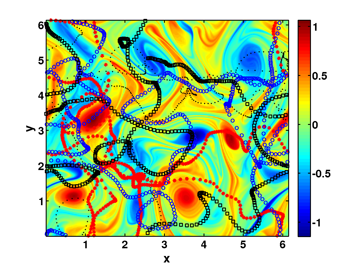
Figure 1: (Color online) Representative particle trajectories of a Lagrangian tracer (black line) and three different heavy particles with ${\rm St}=0.1$ (red asterisks), ${\rm St}=0.5$ (blue circles), and ${\rm St}=1$ (black squares) superimposed on a pseudocolor plot of ${\bm{\omega}}$. For the spatiotemporal evolution of this plot see the animation available at the location http://www.youtube.com/watch?v=lk3iSHhfTuU

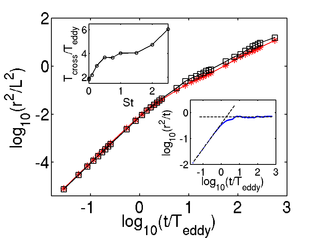
Figure 2: (Color online) Log-log (base 10) plots of $r^{2}$ versus $t/T_{\rm eddy}$ for ${\rm St}=0.1$ (red triangles), and ${\rm St}=1$ (black squares); top inset: plot of $T_{\rm cross}/T_{\rm eddy}$ versus ${\rm St}$; bottom inset: log-log (base 10) plot of $r^{2}/t$ versus $t/T_{\rm eddy}$ for tracers (blue curve) and linear fits to the small- and large-$t$ asymptotes (dashed lines) with slopes $1$ and $0$ in ballistic and Brownian regimes, respectively; the intersection point of these dashed lines yields $T_{\rm cross}$.

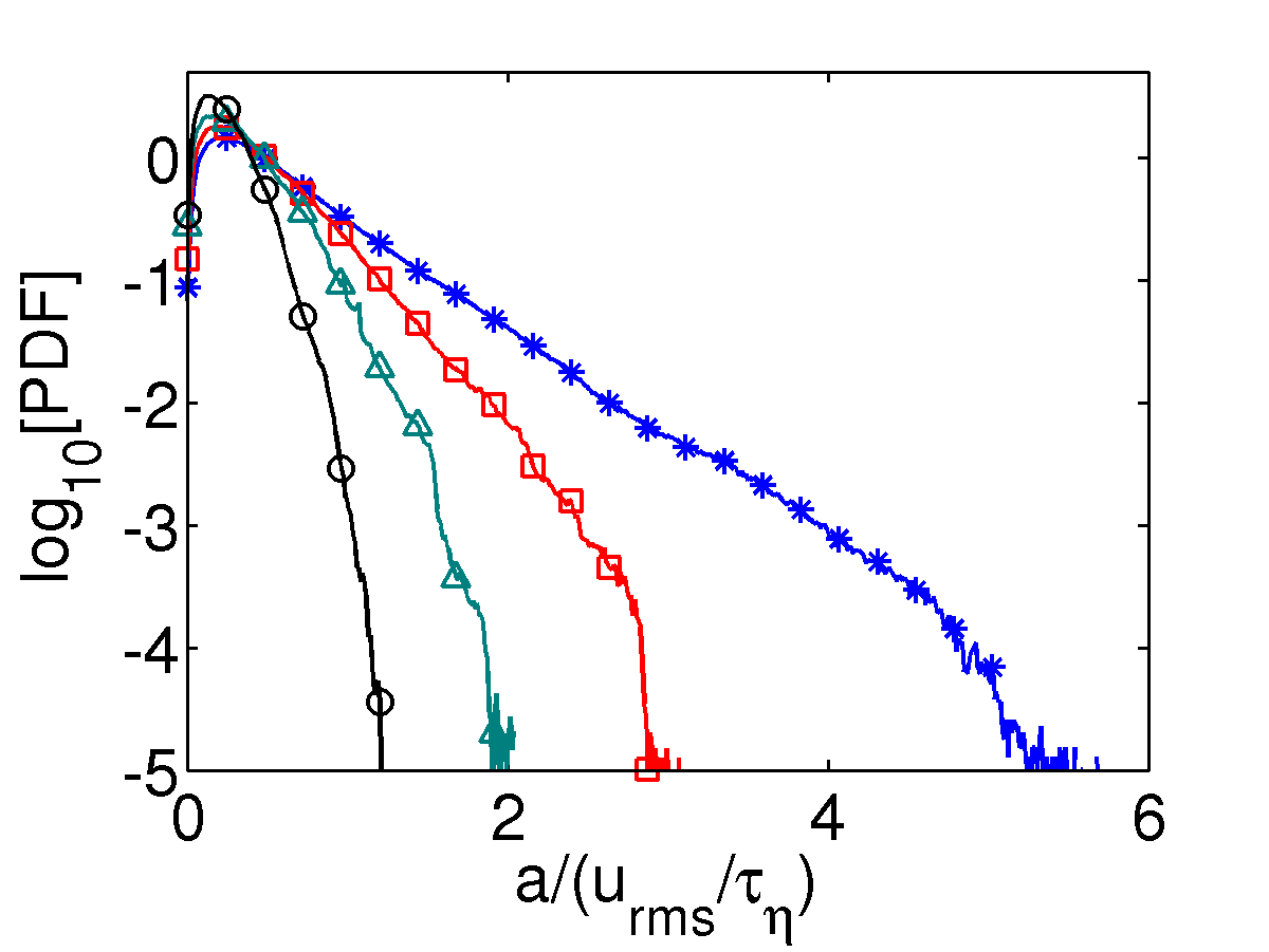
Figure 3: (Color online) Plots of PDFs of (a) the modulus of $a$ of the particle acceleration, (b) its tangential component $a_{t}$, and (c) its normal component $a_{n}$ for ${\rm St}=0$ (blue curve), $0.5$ (red curve), $1$ (green curve), and $2$ (black curve).

In Fig. (3) we present semilog plots of the PDFs $\mathcal{P}(a)$, $\mathcal{P}(a_{t})$, and $\mathcal{P}(a_{n})$ for some representative values of ${\rm St}$. Clearly, all of these PDFs have exponential tails, i.e., $\mathcal{P}(a,{\rm St})\sim\exp[-a/\alpha({\rm St})]$, $\mathcal{P}(a_{t},{\rm St})\sim\exp[-a_{t}/\alpha_{\rm t}({\rm St})]$, and $\mathcal{P}(a_{n},{\rm St})\sim\exp[-a_{n}/\alpha_{\rm n}({\rm St})]$. As ${\rm St}$ increases, the tails of these PDFs fall more and more rapidly, because the higher the inertia the more difficult is it to accelerate a particle. Hence, $\alpha$, $\alpha_{\rm t}$, and $\alpha_{\rm n}$ decrease with ${\rm St}$ [see Table (2)].

Although these acceleration PDFs have exponential tails, $\mathcal{P}(\kappa)$ shows a power-law behavior as $\kappa\to\infty$, as we have mentioned above. The exponent $h_{\rm r}$ for the right-tail of $\mathcal{P}(\kappa)$ is especially interesting because it characterizes the parts of a trajectory that have large values of $\kappa$. If $\mathcal{P}(\kappa)\sim\kappa^{-h_{\rm r}}$, then its cumulative PDF $\mathcal{Q}(\kappa)\sim\kappa^{-h_{\rm r}+1}$. We obtain an accurate estimate of $h_{\rm r}$ from $\mathcal{Q}$, which we obtain by a rank-order method that does not suffer from binning errors mit05a . We give representative, log-log plots of $\mathcal{Q}$ in Fig. (4), for ${\rm St}=0.1$ (blue asterisks) and ${\rm St}=1$ (red squares); and we determine $h_{\rm r}$ by fitting a straight line to $\mathcal{Q}$ over a scaling range of more than two decades; We plot, in the inset, Fig. (4), the local slope of this scaling range, whose mean value and standard deviation yield, respectively, $h_{\rm r}$ and its error bars. From such plots we find that $h_{\rm r}$ does not depend significantly on ${\rm St}$ [Table (2)]. Furthermore, we find that the Lagrangian analog of $h_{\rm r}$, which we denote by $h_{\rm lagrangian}$, is $2.03\pm 0.09$, i.e., it lies within error bars of $h_{\rm r}$. By analyzing the $\kappa\to 0$ limit of $\mathcal{P}(\kappa)$, we find that $\mathcal{P}(\kappa)\sim A_{0}\kappa^{h_{\rm l}}$, where $A_{0}>0$ is an amplitude and $h_{\rm l}=0.0\pm 0.1$ (the latter is independent of ${\rm St}$); this indicates that there is a nonzero probability that the paths of particles have zero curvature, i.e., they can move in straight lines. The $\kappa\to 0$ limit of $\mathcal{P}(\kappa)$ seems, therefore, to be different from its counterpart for 3D fluid turbulence (see Ref. xu+oue+bod07 for Lagrangian tracers and Ref. akshaypreprint for heavy particles), where $\mathcal{P}(\kappa)\to 0$ as $\kappa\to 0$. Very-high-resolution DNSs for 2D turbulence must be undertaken to probe the $\kappa\to 0$ limit of $\mathcal{P}(\kappa)$ by going to even smaller values of $\kappa$ than we have been able to obtain reliably in our DNS.

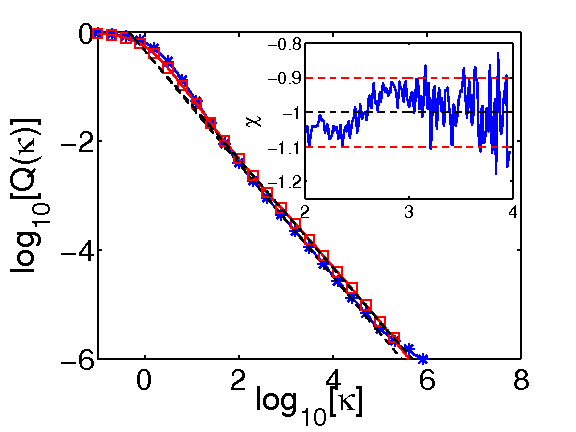
Figure 4: (Color online) Log-log plots of the cumulative PDFs $\mathcal{Q}(\kappa)$ for ${\rm St}=0.1$ (blue asterisks) and ${\rm St}=1$ (red squares); the inset shows a plot of the local slope of the tail of this cumulative PDF and the two dashed horizontal lines indicate the maximum and minimum values of this local slope in the range we use for fitting the exponent $h_{\rm r}$.

A point in a 2D flow is vortical or strain-dominated if the Okubo-Weiss parameter $\Lambda=(1/8)(\omega^{2}-\sigma^{2})$ is, respectively, positive or negative oku70 ; wei91 ; per+ray+mit+pan11 . We now investigate how the acceleration statistics of heavy particles depends on the sign of $\Lambda$ by conditioning the PDFs of $a_{t}$ and $\kappa$ on this sign. In particular, we obtain the conditional PDFs $\mathcal{P}^{+}$ and $\mathcal{P}^{-}$, where the superscript stands for the sign of $\Lambda$. We find, on the one hand, that the tail of $\mathcal{P}^{+}(a_{t})$ falls faster than that of $\mathcal{P}^{-}(a_{t})$ because regions of the trajectory with high tangential accelerations are associated with strain-dominated points in the flow. On the other hand, the right tail of $\mathcal{P}^{+}(\kappa)$ falls more slowly than that of $\mathcal{P}^{-}(\kappa)$, which implies that high-curvature parts of a particle trajectory are correlated with vortical regions of the flow. We give plots of $\mathcal{P}^{+}(a_{t})$, $\mathcal{P}^{+}(\kappa)$, $\mathcal{P}^{-}(a_{t})$, and $\mathcal{P}^{-}(\kappa)$ in the Appendix A.

We find that ${\bm{a}}\times{\bm{v}}$ (a pseudoscalar in 2D like the vorticity) changes sign at several inflection points along a particle trajectory. We use the number of inflection points on a trajectory, per unit time, $n_{\rm I}({\rm St})$ (see Eq. (1)) as a measure of its complexity. In Fig. (5) we demonstrate that the limit in Eq. (1) exists by plotting $N_{\rm I}(t,{\rm St})/t$ as a function of $t$ for ${\rm St}=0.1$ (red asterisks) and ${\rm St}=2$ (black triangles); the mean value of $N_{\rm I}(t,{\rm St})/t$, between the two vertical dashed lines in Fig. (5), yields our estimate for $n_{\rm I}({\rm St})$, which is given in the inset as a function of ${\rm St}$ (on a log-log scale); the standard deviation gives the error bars. From this inset of Fig. (5) we conclude that $n_{\rm I}({\rm St})\sim{\rm St}^{-\Delta},$ with $\Delta=0.33\pm 0.05$. This exponent $\Delta$ [Table (1)] is independent of the Reynolds number and $\mu$, within the range of parameters we have explored. Furthermore, $\Delta$ is independent of whether our 2D turbulent flow is dominated by forward or the inverse cascades in $E(k)$, which are controlled by $k_{\rm inj}$.

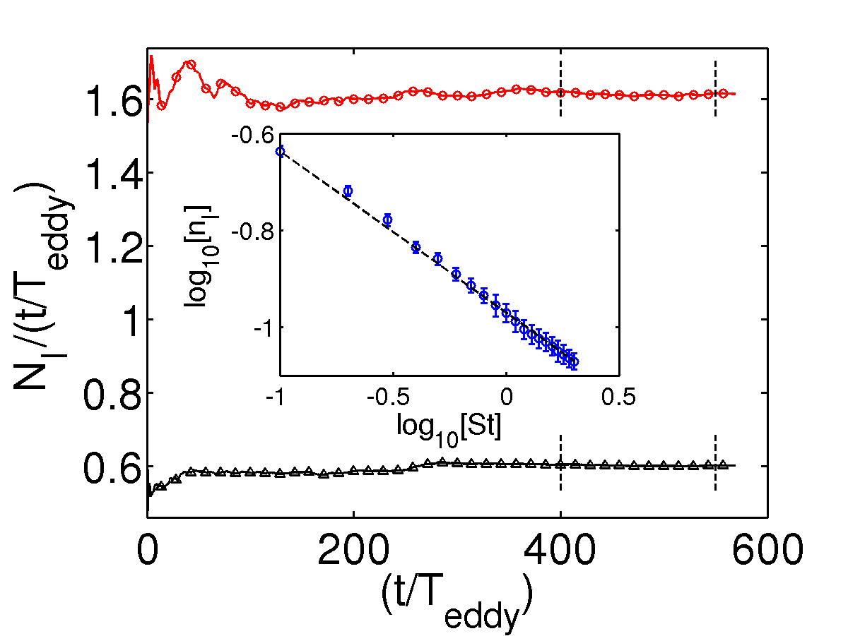
Figure 5: (Color online) Plots of $N_{\rm I}/(t/T_{\rm eddy})$ versus $t/T_{\rm eddy}$ for ${\rm St}=0.1$ (red curve) and ${\rm St}=2$ (black curve); the inset shows a log-log (base 10) plot of $n_{\rm I}$ versus ${\rm St}$ (blue open circles); the black dotted line has a slope $=-1/3$.

We have repeated all the above studies with a forcing term that yields an energy spectrum with a significant inverse-cascade part ($k_{\rm inj}=50$); the parameters for this run are given in Table (1) in the Appendix A and in Ref. AGthesis . The dependence of all the tails of the PDFs discussed above and the exponents $h_{\rm l}$ and $h_{\rm r}$ on ${\rm St}$ are similar to those we have found above for $k_{\rm inj}=4$.

Earlier studies of the geometrical properties of particle tracks have been restricted to tracers; and they have inferred these properties from tracer velocities and accelerations. For example, the PDFs of different components of the acceleration of Lagrangian particles in 2D turbulent flows has been studied for both decaying wil+kam+fri08 and forced kad+del+bos+sch11 cases; they have shown exponential tails in periodic domains, but, in a confined domain, have obtained PDFs with heavier tails kad+bos+sch08 . The PDF of the curvature of tracer trajectories has been calculated from the same simulations, which quote an exponent $h_{\rm lagrangian}\simeq 2.25$ (but no error bars are given). Our work goes well beyond these earlier studies by (a) investigating the statistical properties of the geometries of the trajectories of heavy particles in 2D turbulent flows for a variety of parameter ranges and Stokes numbers, (b) by introducing and evaluating, with unprecedented accuracy (and error bars), the exponent $h_{\rm r}$, (c) proposing $n_{\rm I}$ as a measure of the complexity of heavy-particle trajectories and obtaining the exponent $\Delta$ accurately, (d) by examining the dependence of all these exponents on ${\rm St}$ and $k_{\rm inj}$, and (e) showing, thereby, that these exponents are universal (within our error bars).

Our results imply that $n_{\rm I}({\rm St})$ has a power-law divergence, so the trajectories become more and more contorted, as ${\rm St}\to 0$. This divergence is suppressed eventually, in any DNS, which can only achieve a finite value of $Re_{\lambda}$ because it uses only a finite number of collocation points. Such a suppression is the analog of the finite-size rounding off of divergences, in say the susceptibility, at an equilibrium critical point fssprivman . Note also that the limit ${\rm St}\to 0$ is singular and it is not clear a priori that this limit should yield the same results, for the properties we study, as the Lagrangian case ${\rm St}=0$.

We hope that our study will lead to experimental studies and accurate measurements of the exponents $h_{\rm r}$ and $\Delta$, and applications of these in developing a detailed understanding of particle-laden flows in the variety of systems that we have mentioned in the introduction.

For 3D turbulent flows, geometrical properties of Lagrangian-particle trajectories have been studied numerically bra+lil+eck06 ; sca11 and experimentally xu+oue+bod07 . However, such geometrical properties have not been studied for heavy particles. The extension of our heavy-particle study to the case of 3D fluid turbulence is nontrivial and will be given in a companion paper akshaypreprint .

$Run$	$N$	$F_{0}$	$k_{\rm inj}$	$\ell_{\rm d}$	$\lambda$	$Re_{\lambda}$	$T_{\rm eddy}$	$T_{\eta}$	$T_{\rm inj}$
IA	$1024$	$0.2$	$50$	$1.3\times 10^{-3}$	$0.06$	$1219$	$0.98$	$0.16$	$2.94$
FA	$1024$	$0.005$	$4$	$5.4\times 10^{-3}$	$0.2$	$1322$	$7$	$2.9$	$30.2$

Table 1: The parameters for our DNS runs: $N^{2}$ is the number of collocation points, $N_{\rm p}=10^{4}$ is the number of Lagrangian or inertial particles, $\delta t$ the time step, $\nu=10^{-5}$ the kinematic viscosity, and $\mu=0.01$ the air-drag-induced friction, $F_{0}$ the forcing amplitude, $k_{\rm inj}$ the forcing wave number, $l_{d}\equiv(\nu^{3}/\varepsilon)^{1/4}$ the dissipation scale, $\lambda\equiv\sqrt{\nu E/\varepsilon}$ the Taylor microscale, $Re_{\lambda}=u_{\rm rms}\lambda/\nu$ the Taylor-microscale Reynolds number, $T_{eddy}=(\frac{\sum_{k}E(k)/k}{\sum_{k}E(k)})/u_{rms}$ the eddy-turn-over time, and $T_{\eta}\equiv\sqrt{(\nu/\varepsilon)}$ the Kolmogorov time scale. $T_{\rm inj}\equiv(\ell_{\rm inj}^{2}/E_{\rm inj})^{1/3}$ is the energy-injection time scale, where $E_{\rm inj}=<{\bf f_{\rm u}}\cdot{\bm{u}}>$, is the energy-injection rate, $\ell_{\rm inj}=2\pi/k_{\rm inj}$ is the energy-injection length scale, and ${\bm{f}}_{\omega}=\nabla\times{\bm{f}}_{\rm u}$.

$Run$	${\rm St}$	$\alpha$	$\alpha_{\rm t}$	$\alpha_{\rm n}$	$h_{\rm r}$
F1	$0.1$	$0.86\pm 0.07$	$1.45\pm 0.07$	$0.86\pm 0.07$	$2.03\pm 0.08$
F2	$0.2$	$0.96\pm 0.06$	$1.66\pm 0.07$	$0.97\pm 0.06$	$2.0\pm 0.1$
F3	$0.3$	$1.11\pm 0.07$	$1.87\pm 0.07$	$1.12\pm 0.06$	$2.0\pm 0.1$
F4	$0.4$	$1.43\pm 0.07$	$2.15\pm 0.07$	$1.36\pm 0.09$	$2.04\pm 0.09$
F5	$0.5$	$1.56\pm 0.08$	$2.27\pm 0.08$	$1.45\pm 0.09$	$2.0\pm 0.1$
F6	$0.6$	$1.66\pm 0.08$	$2.36\pm 0.09$	$1.6\pm 0.1$	$2.02\pm 0.09$
F7	$0.7$	$1.88\pm 0.09$	$2.51\pm 0.09$	$1.61\pm 0.09$	$2.06\pm 0.09$
F8	$0.8$	$2.22\pm 0.08$	$2.73\pm 0.09$	$1.90\pm 0.09$	$2.01\pm 0.08$
F9	$0.9$	$2.6\pm 0.1$	$2.9\pm 0.1$	$2.0\pm 0.1$	$2.0\pm 0.1$
F10	$1.0$	$2.6\pm 0.1$	$3.3\pm 0.1$	$2.17\pm 0.09$	$2.0\pm 0.1$
F11	$1.5$	$3.9\pm 0.1$	$4.3\pm 0.1$	$3.3\pm 0.1$	$2.1\pm 0.1$
F12	$2.0$	$4.5\pm 0.1$	$4.7\pm 0.1$	$3.8\pm 0.1$	$2.0\pm 0.1$

Table 2: The values of $\alpha$, $\alpha_{\rm n}$, and $\alpha_{\rm t}$ and the exponent $h_{\rm r}$ for the case $k_{\rm inj}=4$ and for different values of ${\rm St}$.

I Acknowledgments

We thank A. Bhatnagar, A. Brandenburg, B. Mehlig, S.S. Ray, and D. Vincenzi for discussions, and particularly A. Niemi, whose study of the intrinsic geometrical properties of polymers poly11 , inspired our work on particle trajectories. The work has been supported in part by the European Research Council under the AstroDyn Research Project No. 227952 (DM), Swedish Research Council under grant 2011-542 (DM), NORDITA visiting PhD students program (AG), and CSIR, UGC, and DST (India) (AG and RP). We thank SERC (IISc) for providing computational resources. AG, PP, and RP thank NORDITA for hospitality; DM thanks the Indian Institute of Science for hospitality.

*

Appendix A Statistical Properties of the Intrinsic Geometry of Heavy-particle Trajectories in Two-dimensional, Homogeneous, Isotropic Turbulence : Supplemental Material

In this Supplemental Material we provide numerical details of our direct numerical simulation (DNS) of Eq. (2) in the main part of this paper. We also give results of our DNS for the case of the injection wave vector $k_{\rm inj}=50$, which yields a significant inverse-cascade part in the energy spectrum $E(k)$. In Fig. (6) we show the energy spectra $E(k)$ for our runs $\tt FA$ ($k_{\rm inj}=4$) and $\tt IA$ ($k_{\rm inj}=50$).

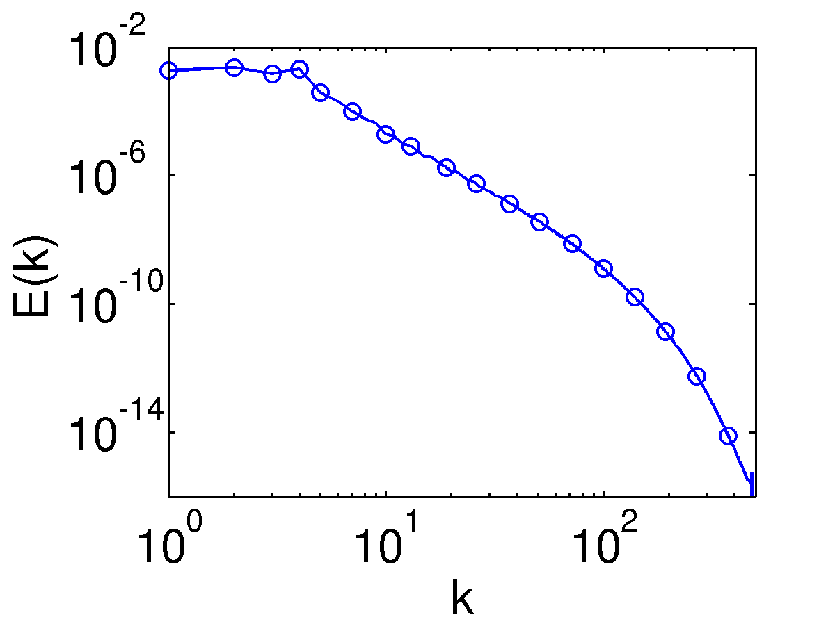
Figure 6: (Color online) Log-log (base 10) plots of the energy spectra $E(k)$ versus $k$ for (a) runs $\tt FA$ ($k_{\rm inj}=4$) and (b) runs $\tt IA$ ($k_{\rm inj}=50$).

We perform a DNS of Eq. (2) by using a pseudo-spectral code Can88 with the $2/3$ rule for dealiasing; and we use a second-order, exponential time differencing Runge-Kutta method cox+mat02 for time stepping. We use periodic boundary conditions in a square simulation domain with side $\mathbb{L}=2\pi$, with $N^{2}$ collocation points. Together with Eq.(2) we solve for the trajectories of $N_{\rm p}$ heavy particles, for each of which we solve Eq. (4) with an Euler scheme. The use of an Euler scheme to evolve particles is justified because, in time $\delta t$, a particle crosses at most one-tenth of grid spacing. We obtain the Lagrangian velocity at an off-grid particle position ${\bm{x}}$, from the Eulerian velocity field by using a bilinear-interpolation scheme Pre+Fla+Teu+Vet92 ; for numerical details see Refs. per+pan09 ; Per09 ; per+ray+mit+pan11 ; ray+mit+per+pan11 .

We calculate the fluid energy-spectrum $E(k)\equiv\sum_{k-1/2<k^{\prime}\leq k+1/2}k^{\prime 2}\langle|\hat{\psi}({\bf k^{\prime}},t)|^{2}\rangle_{t}$, where $\langle\cdot\rangle_{t}$ indicates a time average over the statistically steady state. The parameters in our simulations are given in Table(II) of the main part of this paper and in Table(3). These include the Taylor-microscale Reynolds number, $Re_{\lambda}\equiv u_{\rm rms}\lambda/\nu$, where $\lambda\equiv\sqrt{\nu E/\varepsilon}$ is the Taylor microscale and the Stokes number ${\rm St}=\tau_{\rm s}/T_{\eta}$. We use $20$ different values of ${\rm St}$ to study the dependence on ${\rm St}$ of the PDFs $\mathcal{P}(a)$, $\mathcal{P}(a_{t})$ and $\mathcal{P}(a_{n})$, the cumulative PDF $\mathcal{Q}(\kappa)$, the mean square displacement, and the number of inflection points $N_{\rm I}(t,{\rm St})$ at which ${\bm{a}}\times{\bm{v}}$ changes sign along a particle trajectory.

A point in a 2D flow is vortical or strain-dominated if the Okubo-Weiss parameter $\Lambda=(1/8)(\omega^{2}-\sigma^{2})$ is, respectively, positive or negative oku70 ; wei91 ; per+ray+mit+pan11 . We investigate how the acceleration statistics of heavy particles depends on the sign of $\Lambda$ by conditioning the PDFs of $a_{t}$ and $\kappa$ on this sign. In particular, we obtain the conditional PDFs $\mathcal{P}^{+}$ and $\mathcal{P}^{-}$, where the superscript stands for the sign of $\Lambda$. We find, on the one hand, that the tail of $\mathcal{P}^{+}(a_{t})$ falls faster than that of $\mathcal{P}^{-}(a_{t})$ because regions of the trajectory with high tangential accelerations are associated with strain-dominated points in the flow. On the other hand, the right tail of $\mathcal{P}^{+}(\kappa)$ falls more slowly than that of $\mathcal{P}^{-}(\kappa)$, which implies that high-curvature parts of a particle trajectory are correlated with vortical regions of the flow. We give plots of $\mathcal{P}^{+}(a_{t})$, $\mathcal{P}^{+}(\kappa)$, $\mathcal{P}^{-}(a_{t})$, and $\mathcal{P}^{-}(\kappa)$ in Fig. (7) and Fig. (8). These trends hold for all values of ${\rm St}$ and $k_{\rm inj}$ that we have studied.

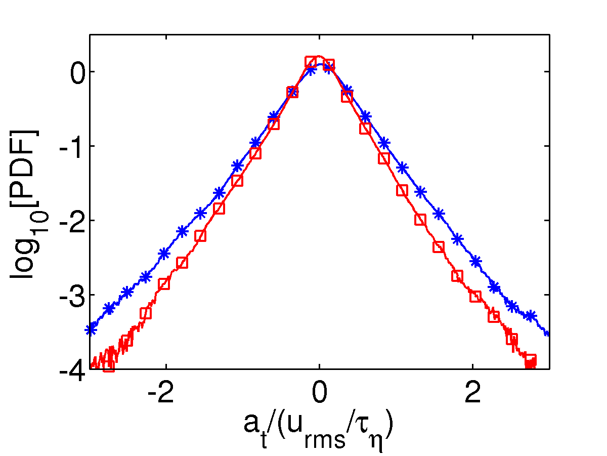
Figure 7: (Color online) Semilog (base 10) plots of the PDFs of the tangential component of the acceleration for ${\rm St}=0.1$ in vortical regions $\mathcal{P}(a_{t}^{+})$ (red squares) and in strain-dominated regions $\mathcal{P}(a_{t}^{-})$ (blue asterisks).

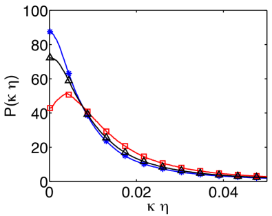
Figure 8: (Color online) Semilog (base 10) plots of PDF of the curvature of trajectories for ${\rm St}=0.1$ in vortical regions $\mathcal{P}(\kappa^{+}\eta)$ (red squares), in strain-dominated regions $\mathcal{P}(\kappa^{-}\eta)$ (blue asterisks), and in general (i.e., without conditioning on the sign of $\Lambda$) $\mathcal{P}(\kappa\eta)$ (black triangles).

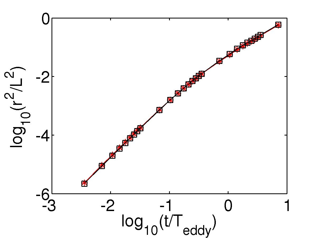
Figure 9: (Color online) Log-log (base 10) plots for $k_{\rm inj}=50$ of $r^{2}$ versus $t/T_{\rm eddy}$ for ${\rm St}=0.1$ (red asterisks) and ${\rm St}=1$ (black squares).

In Fig. (9), we plot the square of the mean-squared displacement $r^{2}$ versus time $t$ for $k_{\rm inj}=50$; here too we see a crossove from ballistic to Brownian behaviors; however, in contrast to the case $k_{\rm inj}=4$, the crossover time $T_{\rm cross}$ does not depend significantly on ${\rm St}$.

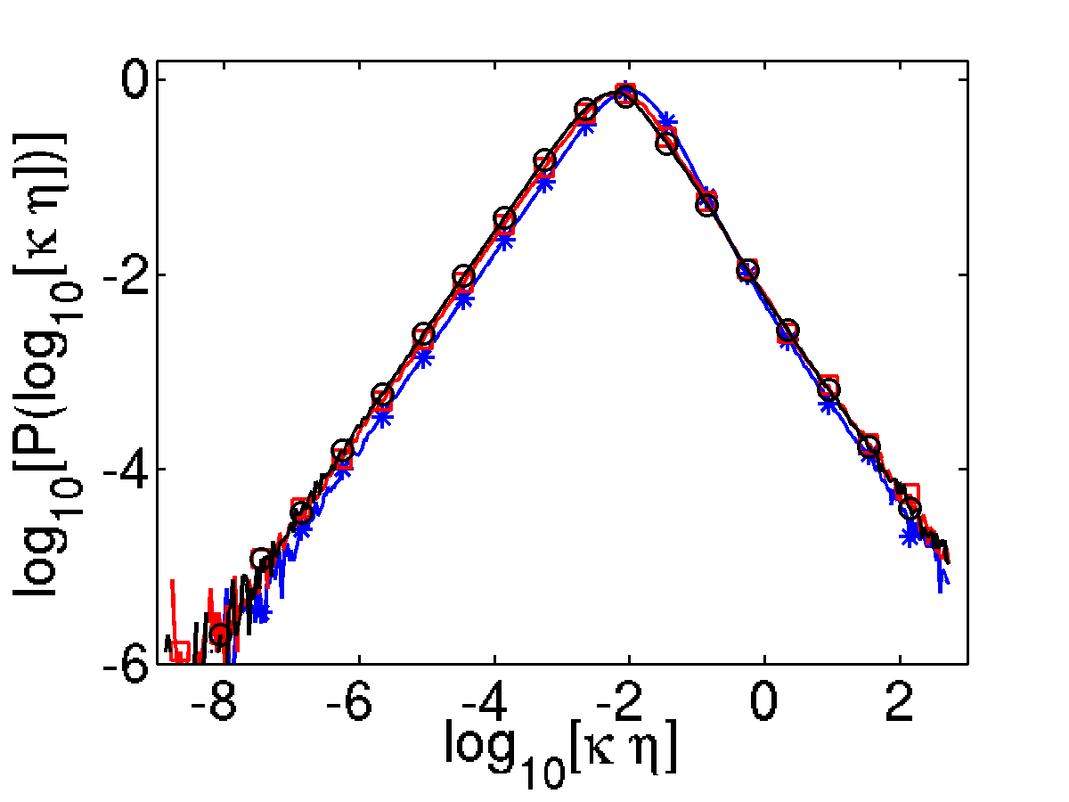
Figure 10: (Color online) Semilog (base 10) plot of the PDF $\mathcal{P}(\log_{10}(\kappa\eta))$ versus $\log_{10}(\kappa\eta)$, for ${\rm St}=0.1$ (blue asterisks), 301 ${\rm St}=1$ (red squares) and ${\rm St}=2$ (black circles).

In Fig. (10), we plot the PDF $\mathcal{P}(\log_{10}(\kappa\eta))$ versus $\log_{10}(\kappa\eta)$, for ${\rm St}=0.1$ (blue asterisks), ${\rm St}=1$ (red squares) and ${\rm St}=2$ (black circles). Such PDFs provide another convenient way of displaying the power-law behaviors, as $\kappa\to\infty$ and $\kappa\to 0$, which we have reported in the main part of this paper, where we have used the cumulative PDF of $\kappa$ to obtain the power-law exponents.

In Table(3) we report the values of $\alpha$, $\alpha_{\rm n}$, $\alpha_{\rm t}$, and the exponent $h_{\rm r}$ of the right tail of the PDF of the trajectory curvature, for the case $k_{\rm inj}=50$ and for different values of ${\rm St}$.

$Run$	${\rm St}$	$\alpha$	$\alpha_{\rm t}$	$\alpha_{\rm n}$	$h_{\rm r}$
I1	$0.1$	$0.39\pm 0.06$	$0.69\pm 0.02$	$0.40\pm 0.06$	$2.16\pm 0.09$
I2	$0.2$	$0.47\pm 0.05$	$0.81\pm 0.03$	$0.46\pm 0.05$	$2.14\pm 0.09$
I3	$0.3$	$0.55\pm 0.04$	$0.95\pm 0.02$	$0.54\pm 0.05$	$2.1\pm 0.1$
I4	$0.4$	$0.63\pm 0.04$	$1.09\pm 0.03$	$0.61\pm 0.04$	$2.10\pm 0.08$
I5	$0.5$	$0.71\pm 0.04$	$1.21\pm 0.02$	$0.68\pm 0.03$	$2.09\pm 0.09$
I6	$0.6$	$0.80\pm 0.03$	$1.34\pm 0.03$	$0.77\pm 0.03$	$2.08\pm 0.09$
I7	$0.7$	$0.88\pm 0.04$	$1.48\pm 0.04$	$0.85\pm 0.03$	$2.07\pm 0.09$
I8	$0.8$	$0.97\pm 0.03$	$1.60\pm 0.03$	$0.94\pm 0.04$	$2.07\pm 0.09$
I9	$0.9$	$1.05\pm 0.03$	$1.73\pm 0.03$	$1.01\pm 0.04$	$2.1\pm 0.1$
I10	$1.0$	$1.16\pm 0.03$	$1.87\pm 0.03$	$1.10\pm 0.03$	$2.1\pm 0.1$

Table 3: The values of $\alpha$, $\alpha_{\rm n}$, $\alpha_{\rm t}$, and the exponent $h_{\rm r}$, for the case $k_{\rm inj}=50$ for different values of ${\rm St}$.

In Table(4) we report the exponent $h_{\rm l}$, which charcterizes $\mathcal{P}(\kappa\eta)$, as $\kappa\to 0$, in both the cases $k_{\rm inj}=4$ and $k_{\rm inj}=50$. In both these cases and for all the different values of ${\rm St}$ we have studied, $h_{\rm l}=0.0\pm 0.1$.

${\rm St}$	$0.1$	$0.2$	$0.3$	$0.4$	$0.5$	$1.0$
$h_{\rm l}$ ($\tt FA$)	$0.0\pm 0.1$	$0.0\pm 0.1$	$0.0\pm 0.1$	$0.0\pm 0.1$	$0.0\pm 0.1$	$0.0\pm 0.1$
$h_{\rm l}$ ($\tt IA$)	$0.0\pm 0.1$	$0.0\pm 0.1$	$0.0\pm 0.1$	$0.0\pm 0.1$	$0.0\pm 0.1$	$0.0\pm 0.1$

Table 4: The exponent $h_{\rm l}$ that charcterizes $\mathcal{P}(\kappa\eta)$, as $\kappa\to 0$, in both the cases $k_{\rm inj}=4$ and $k_{\rm inj}=50$ and for different values of ${\rm St}$.

References

- (1) G. Taylor, Proc. London. Math. Soc. s2-20, 196 (1922).
- (2) F. Toschi and E. Bodenschatz, Ann. Rev. Fluid Mech. 41, 375 (2009).
- (3) R. A. Shaw, Annual Review of Fluid Mechanics 35, 183 (2003).
- (4) W. W. Grabowski and L.-P. Wang, Ann. Rev. Fluid Mech. 45, 293 (2013).
- (5) G. Falkovich, A. Fouxon, and M. Stepanov, Nature, London 419, 151 (2002).
- (6) P. J. Armitage, Astrophysics of Planet Formation (Cambridge University Press, Cambridge, UK, 2010).
- (7) G. T. Csanady, Turbulent Diffusion in the Environmnet (Springer, ADDRESS, 1973), Vol. 3.
- (8) J. Eaton and J. Fessler, Intl. J. Multiphase Flow 20, 169 (1994).
- (9) S. Post and J. Abraham, Intl. J. Multiphase Flow 28, 997 (2002).
- (10) G. Falkovich, K. Gawȩdzki, and M. Vergassola, Rev. Mod. Phys. 73, 913 (2001).
- (11) J. Bec, et al., Phys. Fluids 18, 091702 (2006).
- (12) R. Kraichnan and D. Montgomery, Rep. Prog. Phys. 43, (1980).
- (13) R. Pandit, P. Perlekar, and S.S. Ray, Pramana 73, 179 (2009).
- (14) G. Boffetta and R. E. Ecke, Ann. Rev. Fluid Mech. 44, 427 (2012).
- (15) D. Mitra, J. Bec, R. Pandit, and U. Frisch, Phys. Rev. Lett 94, 194501 (2005).
- (16) P. Perlekar, S.S. Ray, D. Mitra, and R. Pandit, Phys. Rev. Lett 106, 054501 (2011).
- (17) A. Okubo, Deep-Sea. Res. 17, 445 (1970).
- (18) J. Weiss, Physica (Amsterdam) 48D, 273 (1991).
- (19) M. R. Maxey and J. J. Riley, Physics of Fluids 26, 883 (1983).
- (20) A. Gupta, PhD. Thesis, Indian Institute of Science, unpublished (2014).
- (21) M. Wilczek, O. Kamps, and R. Friedrich, Physica D: Nonlinear Phenomena 237, 2090 (2008).
- (22) B. Kadoch, D. del Castillo-Negrete, W. J. T. Bos, and K. Schneider, Phys. Rev. E 83, 036314 (2011).
- (23) B. Kadoch, W. J. T. Bos, and K. Schneider, Phys. Rev. Lett. 100, 184503 (2008).
- (24) W. Braun, F. De Lillo, and B. Eckhardt, Journal of Turbulence 7, (2006).
- (25) A. Scagliarinia, Journal of Turbulence, 12, N25, (2011); DOI: 10.1080/14685248.2011.571261.
- (26) H. Xu, N.T. Ouellette, and E. Bodenschatz, Physical Review Letters 98, 050201 (2007).
- (27) See, e.g., V. Privman, in Chapter I in ”Finite Size Scaling and Numerical Simulation of Statistical Systems,” ed. V. Privman (World Scientific, Singapore, 1990) pp 1-98. Finite-size scaling is used to evaluate inifinte-size-system exponents systematically at conventional critical points; its analog for our study requires several DNSs, over a large range of , which lie beyond the scope of our investigation.
- (28) A. Bhatnagar, D. Mitra, A. Gupta, P. Perlekar, and R. Pandit, to be published.
- (29) S. Hu, M. Lundgren, and A.J. Niemi, Phys. Rev. E 83, 061908 (2011)
- (30) C. Canuto, M. Hussaini, A. Quarteroni, and T. Zang, Spectral methods in Fluid Dynamics (Spinger-Verlag, Berlin, 1988).
- (31) S. Cox and P. Matthews, Journal of Computational Physics 176, 430 (2002).
- (32) W. Press, B. Flannery, S. Teukolsky, and W. Vetterling, Numerical Recipes in Fortran (Cambridge University Press, Cambridge, 1992).
- (33) P. Perlekar and R. Pandit, New J. Phys. 11, 073003 (2009).
- (34) P. Perlekar, Ph.D. thesis, Indian Institute of Science, Bangalore, India, 2009.
- (35) S. S. Ray, D. Mitra, P. Perlekar, and R. Pandit, Phys. Rev. Lett. 107, 184503 (2011).
- (36) L. Biferale et al., Phys. Rev. Lett. 93, 064502 (2004).
- (37) J. Bec et al., Journal of Fluid Mechanics 550, 349 (2006).
*