Skyrmion spacetime defect

Abstract

A finite-energy static classical solution is obtained for standard Einstein gravity coupled to an $SO(3)\times SO(3)$ chiral model of scalars [a Skyrme model]. This nonsingular localized solution has nontrivial topology for both the spacetime manifold and the $SO(3)$ matter fields. The solution corresponds to a single spacetime defect embedded in flat Minkowski spacetime.

I Introduction

The classical spacetime emerging from a quantum-spacetime phase may very well have nontrivial structure at small length scales Wheeler1957 ; Wheeler1968 ; Visser1995 . This nontrivial structure affects, in particular, the propagation of electromagnetic waves BernadotteKlinkhamer2006 . The question remains as to what the small-scale structure embedded in a flat spacetime really looks like (here, we do not consider intra-universe wormhole solutions which connect two asymptotically flat spaces Visser1995 ).

Narrowing down the question, is it possible at all to have nonsingular localized finite-energy solutions of the standard Einstein equations with nontrivial topology on small length scales and flat spacetime asymptotically? For one particular topology studied in Ref. BernadotteKlinkhamer2006 , it has been suggested Schwarz2010 to consider an $SO(3)$ Skyrme model coupled to gravity Skyrme1961 ; MantonSutcliffe2004 ; LuckockMoss1986 ; Glendenning-etal1988 ; DrozHeuslerStraumann1991 ; BizonChmaj1992 ; HeuslerStraumannZhou1993 ; KleihausKunzSood1995 .

For this specific theory and topology, two nonsingular defect solutions have been found recently, a vacuum solution and a nonvacuum solution KlinkhamerRahmede2013 . (Corresponding nonsingular black-hole solutions were presented in Refs. Klinkhamer2013-MPLA ; Klinkhamer2013-APPB .) Both defect solutions of Ref. KlinkhamerRahmede2013 are localized, but the one with a nonvanishing scalar $SO(3)$ field has infinite energy and trivial scalar-field-configuration topology (i.e., zero winding number or “baryon” charge). It has been conjectured KlinkhamerRahmede2013 that this particular nonvacuum solution is unstable and, by emitting outgoing waves of scalars, decays to a finite-energy Skyrmion-like defect solution (with unit winding number or “baryon” charge). Such a nonsingular defect solution with unit winding number is constructed in the present article.

The construction of this finite-energy Skyrmion spacetime defect solution turns out to be quite subtle. Essential is a perfect control of the fields at the defect core, which, in turn, requires the use of appropriate coordinates and fields. These preliminaries are discussed in Sec. II. The numerical solution is then given in Sec. III. Concluding remarks are presented in Sec. IV. Two technical issues are dealt with in appendices A and B.

II Theory

The setup of the theory has been described elsewhere in detail KlinkhamerRahmede2013 ; Klinkhamer2013-MPLA ; Klinkhamer2013-APPB ; Klinkhamer2013-review , but, for completeness, we recall the main steps.

II.1 Manifold

The four-dimensional spacetime manifold considered in this article has the topology

$$M_{4}=\mathbb{R}\times M_{3}\,.$$ (1a)

The three-space $$M_{3} M_{3}$$ carries the nontrivial topology and is, in fact, a noncompact, orientable, nonsimply-connected manifold without boundary. Up to a point, is homeomorphic to the three-dimensional real-projective space,

$$M_{3}\simeq\mathbb{R}P^{3}-\{\text{point}\}\,.$$ (1b)

Adding the “point at infinity” gives the compact space $\overline{M_{3}}\simeq\mathbb{R}P^{3}$.

For the direct construction of $M_{3}$, we perform local surgery on the three-dimensional Euclidean space $E_{3}=\big{(}\mathbb{R}^{3},\,\delta_{mn}\big{)}$. We use the standard Cartesian and spherical coordinates on $\mathbb{R}^{3}$,

$$\vec{x}\equiv|\vec{x}|\,\widehat{x}=(x^{1},\,x^{2},\,x^{3})=(r\sin\theta\cos\phi,\,r\sin\theta\sin\phi,\,r\cos\theta)\,,$$ (2)

with $x^{m}\in(-\infty,\,+\infty)$, $r\geq 0$, $\theta\in[0,\,\pi]$, and $\phi\in[0,\,2\pi)$. Now, we obtain $M_{3}$ from $\mathbb{R}^{3}$ by removing the interior of the ball $B_{b}$ with radius $b$ and identifying antipodal points on the boundary $S_{b}\equiv\partial B_{b}$. Denoting point reflection by $P(\vec{x})=-\vec{x}$, the three-space $M_{3}$ is given by

$$M_{3}=\big{\{}\vec{x}\in\mathbb{R}^{3}\,:\;\big{(}|\vec{x}|\geq b>0\big{)}\wedge\big{(}P(\vec{x})\cong\vec{x}\;\;\text{for}\;\;|\vec{x}|=b\big{)}\big{\}}\,,$$ (3)

where $\cong$ stands for pointwise identification (Fig. 1). A minimal noncontractible loop (with length $\pi b$ in $E_{3}$) corresponds to half of a great circle on the $r=b$ sphere in $E_{3}$, taken between antipodal points which are to be identified.

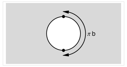
Figure 1: Three-space $M_{3}$ obtained by surgery on three-dimensional Euclidean space $E_{3}$: the interior of the ball with radius $b$ is removed and antipodal points on the boundary of the ball are identified (as indicated by the dots). The “long distance” between antipodal points is $\pi\,b$ in $E_{3}$.

The single set of coordinates (2) does not suffice for an appropriate description of $M_{3}$. The reason is that two different values of these coordinates may correspond to one point of $M_{3}$ as defined in (3). An example is provided by the two sets of coordinates $\vec{x}=(0,\,b,\,0)$ and $\vec{x}=(0,\,-b,\,0)$, which describe the same point of $M_{3}$ (see Fig. 1).

A particular covering of $M_{3}$ uses three charts of coordinates, labeled by $n=1,2,3$. The basic idea Schwarz2010 is that the coordinates resemble spherical coordinates and that each coordinate chart surrounds one of the three Cartesian coordinate axes but does not intersect the other two axes. These coordinates are denoted

$$(X_{n},\,Y_{n},\,Z_{n})\,,$$ (4)

for $n=1,\,2,\,3$. In each chart, there is one polar-type angular coordinate of finite range, one azimuthal-type angular coordinate of finite range, and one radial-type coordinate with infinite range. Specifically, the coordinates have the following ranges:

$$X_{1}\in(-\infty,\,\infty)\,,\quad Y_{1}\in(0,\,\pi)\,,\quad Z_{1}\in(0,\,\pi)\,,$$ (5a)

$$X_{2}\in(0,\,\pi)\,,\quad Y_{2}\in(-\infty,\,\infty)\,,\quad Z_{2}\in(0,\,\pi)\,,$$ (5b)

$$X_{3}\in(0,\,\pi)\,,\quad Y_{3}\in(0,\,\pi)\,,\quad Z_{3}\in(-\infty,\,\infty)\,.$$ (5c)

The different charts overlap in certain regions: see Appendix B of Ref. Klinkhamer2013-APPB for further details.

II.2 Fields and interactions

The spacetime manifold (1) of the previous section is now supplemented with a metric, $g_{\mu\nu}(X)$, whose dynamics is governed by the standard Einstein–Hilbert action. In addition, we consider a scalar field $\Omega(X)\in SO(3)$, with self-interactions determined by a quartic Skyrme term in the matter action Skyrme1961 ; MantonSutcliffe2004 .

The combined action of the pure-gravity sector and the matter sector is given by ($c=\hbar=1$)

$$S[g,\,\Omega]=\int_{M_{4}}d^{4}X\,\sqrt{-g}\,\Bigg{[}\frac{1}{16\pi G_{N}}\>R+\frac{f^{2}}{4}\>\text{tr}\big{(}\omega_{\mu}\,\omega^{\mu}\big{)}+\frac{1}{16e^{2}}\>\text{tr}\Big{(}\left[\omega_{\mu},\,\omega_{\nu}\right]\left[\omega^{\mu},\,\omega^{\nu}\right]\Big{)}\Bigg{]}\,,$$ (6)

in terms of the Ricci curvature scalar $R$ and the effective vector field $\omega_{\mu}\equiv\Omega^{-1}\,\partial_{\mu}\,\Omega$. The kinetic term of the scalar field involves the mass scale $f$. The Skyrme term corresponds to the trace of the square of the commutator $\left[\omega_{\mu},\,\omega_{\nu}\right]$ and has the dimensionless coupling constant $1/e^{2}$.

The $SO(3)\times SO(3)$ global symmetry of the matter sector is realized on the scalar field by the following transformation with constant parameters $S_{L},\,S_{R}\in SO(3)$:

$$\Omega(X)\to S_{L}\cdot\Omega(X)\cdot S_{R}^{-1}\,,$$ (7)

where the central dot denotes matrix multiplication. The generic argument $X$ of the fields $g_{\mu\nu}(X)$ and $\Omega(X)$ and the measure $d^{4}X$ in the integral (6) correspond to one of the three different coordinate charts needed to cover $M_{4}$.

II.3 Ansätze

A spherically symmetric Ansatz for the metric is given by the following line element:

$$ds^{2}\;\Big{|}_{\text{chart-2}} = -\big{[}\widetilde{\mu}(W)\big{]}^{2}\,dT^{2}+\big{(}1-b^{2}/W\big{)}\,\big{[}\widetilde{\sigma}(W)\big{]}^{2}\,(dY_{2})^{2}$$ (8a)

$$+W\Big{[}(dZ_{2})^{2}+\sin^{2}Z_{2}\,(dX_{2})^{2}\Big{]}\,,$$

$$W\;\Big{|}_{\text{chart-2}} \equiv b^{2}+(Y_{2})^{2}\,,$$ (8b)

and similarly for the chart-1 and chart-3 domains Klinkhamer2013-APPB ; Klinkhamer2013-review . The focus on chart-2 coordinates in (8) is purely for cosmetic reasons. Observe that this Ansatz, for finite values of $\widetilde{\sigma}(b^{2})$, sets the “short distance” between the antipodal points of Fig. 1 to zero, while keeping the “long distance” equal to $\pi\,b$.

The scalar field is described by a Skyrmion-type Ansatz Schwarz2010 ; Skyrme1961 ; MantonSutcliffe2004 ,

$$\Omega = \cos\big{[}\widetilde{F}\left(r^{2}\right)\big{]}\;\openone_{3}-\sin\big{[}\widetilde{F}\left(r^{2}\right)\big{]}\;\widehat{x}\cdot\vec{S}+\big{(}1-\cos\big{[}\widetilde{F}\left(r^{2}\right)\big{]}\big{)}\;\widehat{x}\otimes\widehat{x}\,,$$ (9a)

$$\widetilde{F}(b^{2}) = \pi\,,\quad\widetilde{F}(\infty)=0\,,$$ (9b)

$$S_{1} \equiv \left(\begin{array}[]{ccc}0&0&0\\ 0&0&1\\ 0&-1&0\\ \end{array}\right)\,,\quad S_{2}\equiv\left(\begin{array}[]{ccc}0&0&-1\\ 0&0&0\\ 1&0&0\\ \end{array}\right)\,,\quad S_{3}\equiv\left(\begin{array}[]{ccc}0&1&0\\ -1&0&0\\ 0&0&0\\ \end{array}\right)\,,$$ (9l)

with a hedgehog term proportional to $\sin\widetilde{F}$ in (9a) and further terms involving the $3\times 3$ unit matrix $\openone_{3}$ and another matrix which reads in components $(\widehat{x}\otimes\widehat{x})^{ab}=\widehat{x}^{a}\,\widehat{x}^{b}$.

The boundary condition (9b) at $r\equiv|\vec{x}|=b$ sets the hedgehog term $\widehat{x}\cdot\vec{S}$ in (9a) to zero and makes it possible to employ the single coordinate chart (2). Specifically, there is the following equality:

$$\Omega\big{(}r,\,\widehat{x}\big{)}\,\big{|}_{r=b}=-\;\openone_{3}+2\;\widehat{x}\otimes\widehat{x}=\Omega\big{(}r,\,-\widehat{x}\big{)}\,\big{|}_{r=b}\,,$$ (10)

which gives the same scalar field $\Omega$ for antipodal points on the $r=b$ sphere in $\mathbb{R}^{3}$, allowing these antipodal points to be identified in order to obtain $M_{3}$. In order to match the coordinates used for the metric (8), we make the identification $r^{2}=b^{2}+(Y_{2})^{2}$, and the explicit relations between $\widehat{x}$ and $(X_{2},\,Z_{2})$ can be found in Refs. Klinkhamer2013-APPB ; Klinkhamer2013-review .

The Ansatz (9) corresponds to a topologically nontrivial scalar field configuration, a Skyrmion-like configuration with a unit winding number. Having an integer winding number for the scalar field configuration $\Omega(X)\in SO(3)$ occurs because of the homeomorphism $M_{3}+\{\text{point}\}\simeq SO(3)$. In fact, the winding number or topological degree of the compactified map $\Omega:\overline{M}_{3}\to SO(3)$ turns out to be given by MantonSutcliffe2004 ; Schwarz2010

$$\text{deg}[\Omega]=-\frac{2}{\pi}\;\int_{\pi}^{0}d\widetilde{F}\,\sin^{2}(\widetilde{F}/2)=1\,,$$ (11)

where the endpoints of the integral on the right-hand side correspond to boundary conditions (9b).

Alternative Ansätze based on Painlevé–Gullstrand-type coordinates are presented in Appendix A.

II.4 Reduced field equations

At this moment, we introduce the following dimensionless model parameters and dimensionless variables:

$$\widetilde{\eta} \equiv 8\pi\eta\equiv 8\pi\,G_{N}\,f^{2}\,,$$ (12a)

$$w \equiv (e\,f)^{2}\;W=(y_{0})^{2}+y^{2}\,,$$ (12b)

$$y \equiv e\,f\;Y_{2}\,,$$ (12c)

$$y_{0} \equiv e\,f\;b\,.$$ (12d)

Inserting the Ansätze of Sec. II.3 into the Einstein and matter field equations from the action (6) gives the corresponding reduced expressions Glendenning-etal1988 ; Schwarz2010 ; KlinkhamerRahmede2013 . From these equations written in terms of the dimensionless variables (12), we obtain the following three ordinary differential equations (ODEs):

$$\widetilde{\sigma}^{\prime}(w) = \widetilde{\sigma}(w)\;\Big{(}-\Big{[}w-2\widetilde{\eta}\,\Big{(}1+2w-\cos[\widetilde{F}(w)]\Big{)}\,\sin^{2}[\widetilde{F}(w)/2]\Big{]}\,\widetilde{\sigma}(w)^{2}$$ (13a)

$$+w\,\Big{[}1+2\widetilde{\eta}\,\Big{(}2\,w^{3}(1+y_{0}^{2})-2y_{0}^{2}\,(1+y_{0}^{2})(y_{0}^{4}-1)+2w\,y_{0}^{2}\,(3y_{0}^{2}+3y_{0}^{4}-1)$$

$$-w^{2}\,(6y_{0}^{2}+6y_{0}^{4}-1)-2w\cos[\widetilde{F}(w)]\Big{)}\,\widetilde{F}^{\prime}(w)^{2}\Big{]}\Big{)}\Big{/}\Big{(}4w^{2}\Big{)}\,,$$

$$\widetilde{\mu}^{\prime}(w) = \widetilde{\mu}(w)\;\Big{(}\Big{[}w-2\widetilde{\eta}\,\Big{(}1+2w-\cos[\widetilde{F}(w)]\Big{)}\,\sin^{2}[\widetilde{F}(w)/2]\Big{]}\,\widetilde{\sigma}(w)^{2}$$ (13b)

$$+w\,\Big{[}-1+2w\,\widetilde{\eta}\,\Big{(}2+w-2\cos[\widetilde{F}(w)]\Big{)}\,\widetilde{F}^{\prime}(w)^{2}\Big{]}\Big{)}\Big{/}\Big{(}4w^{2}\Big{)}\,,$$

$$\widetilde{F}^{\prime\prime}(w) = \Big{(}\Big{[}3\,\Big{(}1+w-\cos[\widetilde{F}(w)]\Big{)}\sin[\widetilde{F}(w)]-\Big{(}2+w-2\cos[\widetilde{F}(w)]\Big{)}$$ (13c)

$$\times\Big{(}3w-2\widetilde{\eta}(3+6w-3\cos[\widetilde{F}(w)])\sin^{2}[\widetilde{F}(w)/2]\Big{)}\,\widetilde{F}^{\prime}(w)\Big{]}\,\widetilde{\sigma}(w)^{2}$$

$$-6\,w^{2}\,\Big{[}1+\sin[\widetilde{F}(w)]\widetilde{F}^{\prime}(w)\Big{]}\,\widetilde{F}^{\prime}(w)\Big{)}\Big{/}\Big{(}2w^{2}\Big{[}6+3w-6\cos[\widetilde{F}(w)]\Big{]}\Big{)}\,,$$

where the prime stands for differentiation with respect to $w$.

The ODEs (13) are to be solved with the following boundary conditions on the functions $\widetilde{F}(w)$, $\widetilde{\sigma}(w)$, and $\widetilde{\mu}(w)$:

$$\widetilde{F}(y_{0}^{2}) = \pi\,,\quad\widetilde{F}(\infty)=0\,,$$ (14a)

$$\widetilde{\sigma}(\infty) = 1\,,\quad\widetilde{\mu}(\infty)=1\,.$$ (14b)

The three boundary conditions at infinity provide for asymptotic flatness and the boundary condition $\widetilde{F}=\pi$ at the core gives a topologically nontrivial scalar field configuration, as discussed in Sec. II.3.

Different from the ODEs used in Ref. KlinkhamerRahmede2013 , the ODEs in the form presented in (13) have no singularities at the defect core $w=y_{0}^{2}>0$. As such, they are directly amenable to numerical analysis.

III Numerical solution

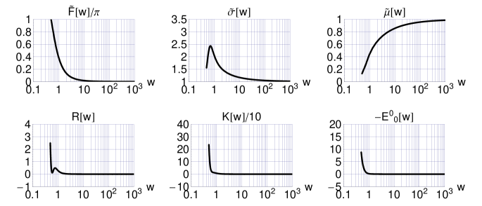
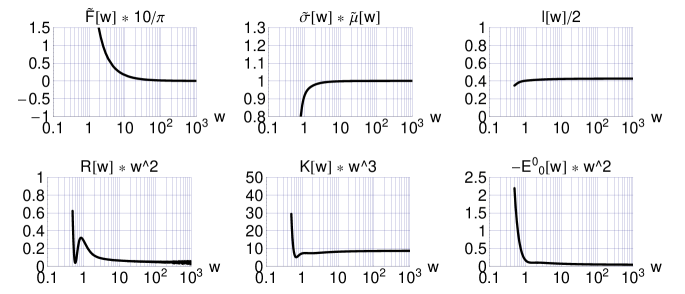
Figure 2: (Top row) Skyrme function $\widetilde{F}(w)$ and metric functions $\widetilde{\sigma}(w)$ and $\widetilde{\mu}(w)$ of the numerical solution of the reduced field equations (13). The model parameter is $\widetilde{\eta}=1/20$ and the solution parameter $y_{0}=1/\sqrt{2}$. The boundary conditions at the defect core $w=y_{0}^{2}=1/2$ are: $\widetilde{F}=\pi$, $\widetilde{F}^{\prime}=-6.3797$, $\widetilde{\sigma}=1.554$, and $\widetilde{\mu}=0.128207$. (Bottom row) Corresponding dimensionless Ricci scalar $R$, dimensionless Kretschmann scalar $K$, and the negative of the 00 component of the dimensionless Einstein tensor $E^{\mu}_{\;\;\nu}$ $\equiv$ $R^{\mu}_{\;\;\nu}-(1/2)\,R\,\delta^{\mu}_{\;\;\nu}$; see Appendix B for details.

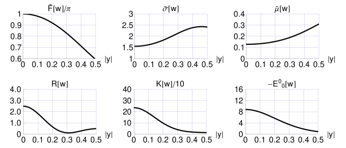
Figure 3: Asymptotic behavior of the functions from Fig. 4, with definition $l(w)\equiv[1-\widetilde{\mu}(w)^{2}]\,\sqrt{w}$.

Figure 4: Core behavior of the functions from Fig. 4, plotted with respect to the dimensionless quasi-radial coordinate $y\in\mathbb{R}$ of the chart-2 domain. The coordinate $w$ is given by $w=y_{0}^{2}+y^{2}$.

In order to obtain the numerical solution corresponding to the Ansätze from Sec. II.3, we have adopted the following procedure. The boundary conditions on the three functions $\widetilde{F}(w)$, $\widetilde{\sigma}(w)$, and $\widetilde{\mu}(w)$ are set at the defect core $w=y_{0}^{2}$. Specifically, we take

$$\widetilde{F}(y_{0}^{2}) = \pi\,,\quad\widetilde{F}^{\prime}(y_{0}^{2})=\alpha\,,$$ (15a)

$$\widetilde{\sigma}(y_{0}^{2}) = \beta\,,\quad\widetilde{\mu}(y_{0}^{2})=\gamma\,,$$ (15b)

for certain initial values $\alpha,\,\beta,\,\gamma\in\mathbb{R}$. With these boundary conditions, the ODEs (13) are solved over $w\in[y_{0}^{2},\,w_{\text{max}}]$ for sufficiently large values of $w_{\text{max}}$. Next, the numbers $\alpha$ and $\beta$ in (15) are varied in order to obtain vanishing $\widetilde{F}(w)$ and $\widetilde{F}^{\prime}(w)$ at $w=w_{\text{max}}$. The obtained function $\widetilde{\mu}(w)$ can then be rescaled in order to obtain at $w=w_{\text{max}}$ the Schwarzschild-type values

$$\widetilde{\sigma}(w_{\text{max}}) \equiv \left(\sqrt{1-l_{\text{max}}/\sqrt{w_{\text{max}}}}\,\right)^{-1}\,,$$ (16a)

$$\widetilde{\mu}(w_{\text{max}}) = \sqrt{1-l_{\text{max}}/\sqrt{w_{\text{max}}}}\,,$$ (16b)

with a dimensionless length parameter $l_{\text{max}}$ set by the value of $\widetilde{\sigma}(w_{\text{max}})$. [An alternative numerical procedure would be to directly use the boundary conditions (14), but then we would have to solve a so-called “two-point boundary value problem” instead of the “initial value problem” from (15).]

Numerical results for the dimensionless gravitational coupling constant $\widetilde{\eta}=1/20$ and the dimensionless defect size $y_{0}=1/\sqrt{2}$ are given in Figs. 4–4. Several comments are in order. First, the results from the bottom row panels in Fig. 4 make clear that the solution is localized. Second, the middle and right panels of the top row in Fig. 4 show the Schwarzschild behavior (16) for $w\gtrsim 10$. Third, it appears that the energy density $-T^{0}_{\;\;0}=-E^{0}_{\;\;0}/\widetilde{\eta}$ from the bottom right panel of Fig. 4 behaves asymptotically as $1/w^{2}\sim 1/|y|^{4}$, which results in a finite energy integral. Fourth, the physical quantities shown in the bottom row of Fig. 4 are nonsingular at the defect core ($y=0$), in accordance with the analytic expressions (19).

Table 1: Numerical results for the dimensionless Schwarzschild mass $\widehat{m}\equiv 4\pi l/\widetilde{\eta}$ in the theory with dimensionless gravitational coupling constant $\widetilde{\eta}=1/20$. The dimensionless length parameter $l$ is obtained from the numerical solution by use of (16b). Also shown are the values of the flat-spacetime energy integral $E^{\text{flat}}$ relative to its Bogomolnyi value $12\,\sqrt{2}\,\pi^{2}\,f/e$. This integral $E^{\text{flat}}$ depends only on the Skyrme function $\widetilde{F}(w)$ and has both metric functions $\widetilde{\sigma}(w)$ and $\widetilde{\mu}(w)$ set to unity; see Appendix B. As such, $E^{\text{flat}}[\widetilde{F}]$ can be used as a diagnostic of the Skyrme function $\widetilde{F}(w)$.

$y_{0}$	$l/2$	$\widehat{m}$	$E^{\text{flat}}/E^{\text{flat}}_{\text{Bogomolnyi}}$
$1/(2\sqrt{2})$	$-$	$-$	$-$
$1/2$	$0.313$	$78.7$	$2.41$
$1/\sqrt{2}$	$0.426$	$107$	$2.27$
$1$	$0.669$	$168$	$1.79$
$\sqrt{2}$	$1.21$	$304$	$1.70$
$2$	$1.58$	$398$	$2.51$

Similar results have been obtained for other values of the dimensionless defect size $y_{0}$, provided they are not too small: $y_{0}>y_{0,\,\text{crit}}$ with $y_{0,\,\text{crit}}\sim 1/(2\sqrt{2})$ for coupling constant $\widetilde{\eta}=1/20$. Table 1 gives the corresponding values for the dimensionless Schwarzschild mass $\widehat{m}$. Qualitatively, these $\widehat{m}$ values agree with those of Fig. 8.7b in Ref. Schwarz2010 , but not quantitatively. This quantitative difference most likely traces back to the fact that the fields of Ref. Schwarz2010 do not solve the Einstein equations at the defect core ($W=b^{2}$ in our notation). This then results in a different behavior of the fields further out, $W>b^{2}$, making for different numerical values of $\widehat{m}$.

The present paper presents only exploratory numerical results, with the sole purpose of establishing the existence of at least one type of Skyrmion-like spacetime-defect solution. For now, two branches of solutions have been found, distinguished by the value of the slope of the Skyrme function at the defect core, $\widetilde{F}^{\prime}(y_{0}^{2})$. The branch with smaller $|\widetilde{F}^{\prime}(y_{0}^{2})|$ has larger Schwarzschild mass $\widehat{m}$ (the numerical results for this branch can be found in a previous version of this paper Klinkhamer2014-v2 ). The branch with larger $|\widetilde{F}^{\prime}(y_{0}^{2})|$ has smaller Schwarzschild mass and the numerical results of this branch have been given in the present paper. More numerical work is clearly needed.

IV Discussion

In this article, we have succeeded in constructing a nonsingular localized finite-energy solution of the standard Einstein equations with nontrivial topology on small length scales and flat spacetime asymptotically. The particular topology is given by (1) and the matter content by a Skyrme model with action (6). The three crucial inputs for obtaining the solution are first, a proper set of coordinates (Sec. II.1); second, appropriate Ansätze (Sec. II.3) and, third, special attention to the behavior of the fields at the defect core for the numerical solution (Sec. III).

This new type of Skyrmion solution is rather interesting: it combines the nontrivial topology of spacetime with the nontrivial topology of field-configuration space. The interplay of spacetime and internal space involves the standard hedgehog behavior (well known from the magnetic-monopole, sphaleron, and standard Skyrmion solutions) and the nontrivial topology of the underlying space manifold allows the internal $SO(3)$ space to be covered only once (see the discussion in Footnote 3).

The Skyrmion defect solution of this paper resembles in certain aspects the defects discussed in brane-world scenarios DvaliKoganShifman2000 ; CembranosDobadoMaroto2002 . But, unlike the brane-Skyrmion of Ref. CembranosDobadoMaroto2002 , our Skyrmion defect solution does not neglect any part of the gravitational interactions, it is a complete solution of the theory considered.

It remains to be proved that the solution obtained in the present article is stable. The scalar fields by themselves would be stable because of the topological charge (11), but, in principle, there could be still more branches of solutions with even lower values of the Schwarzschild mass. A rigorous proof for the stability of the self-gravitating solution would be most welcome. (Equally welcome would be a rigorous proof for the existence of the self-gravitating solution, as we have relied on a numerical analysis of the reduced field equations.)

In Refs. Klinkhamer2013-MPLA ; Klinkhamer2013-APPB , we have given a heuristic discussion on how the corresponding nonsingular black-hole solutions could appear in physical situations of spherical gravitational collapse in an essentially flat spacetime with trivial topology. The scenario is that, when the central matter density becomes large enough, there is a quantum jump Wheeler1957 ; Wheeler1968 from the trivial $\mathbb{R}^{4}$ topology to the nonsimply-connected $M_{4}$ topology of the nonsingular solution, with a noncontractible-loop length scale $b$ of the order of the quantum-gravity length scale $L_{\text{Planck}}$ $\equiv$ $(\hbar\,G_{N}/c^{3})^{1/2}$. (Perhaps topology change is not needed if the nontrivial small-scale topology is already present as a remnant from a quantum spacetime foam Klinkhamer2013-review .)

If a similar discussion applies to the case of the Skyrmion spacetime defect found in this paper, it can be conjectured that defects with the smallest possible value of the mass $\widehat{M}$ would have the largest probability of occurring. For the solutions of Table 1 and setting $\hbar=c=1$, this would imply a preferred value of the defect length scale of approximately $b\equiv y_{0}/(ef)\sim 0.5/(ef)$ for a defect mass of approximately $\widehat{M}\equiv\widehat{m}\,f/e\sim 80\,f/e$, with scalar-field energy scale $f=\sqrt{1/20}\,E_{p}$ in terms of the reduced Planck energy $E_{p}\equiv 1/\sqrt{8\pi\,G_{N}}\approx 2.4\times 10^{18}\,\text{GeV}$.

At this moment, we should mention that the metric (8) of the nonsingular defect solution does have a blemish Klinkhamer2013-MPLA ; Klinkhamer2013-review : at $W=b^{2}$, it cannot be brought to a patch of Minkowski spacetime by a genuine diffeomorphism (a $C^{\infty}$ function) but only by a $C^{1}$ function. This may very well be the price to pay for having a nonsingular solution. The ultimate quantum theory of spacetime and gravity must determine which role (if any) these nonsingular defect-type classical solutions play for the origin of classical spacetime in the very early universe.

Appendix A Alternative Ansätze

In this appendix, we present alternative Ansätze, possibly relevant for nonsingular Skyrmion black-hole solutions with topology (1) and defect length scale $b$.

The new form of the metric Ansatz is related to the one of (8) by the introduction of a new time coordinate, $\widehat{T}=\widehat{T}(T,\,Y_{2})$. This new coordinate follows from considering freely-moving observers falling in along radial geodesics and writing their covariant four-velocities as gradients of a new time function $\widehat{T}$. As such, the procedure is analogous to that of changing the standard coordinates of the Schwarzschild metric to the Painlevé–Gullstrand coordinates Painleve1921 ; Gullstrand1922 ; MartelPoisson2000 , generalized to other static spherically symmetric spacetimes (cf. Sec. IV of Ref. MartelPoisson2000 ).

In this way, we arrive at the following Ansatz for the line element:

$$ds^{2}\;\Big{|}_{\text{chart-2}} = -d\widehat{T}^{2}+\Bigg{[}\widetilde{\chi}(W)\,\frac{Y_{2}}{\sqrt{W}}\;\,dY_{2}+\widetilde{\xi}(W)\,d\widehat{T}\,\Bigg{]}^{2}$$ (17a)

$$+W\Big{[}(dZ_{2})^{2}+\sin^{2}Z_{2}\,(dX_{2})^{2}\Big{]}\,,$$

$$W\;\Big{|}_{\text{chart-2}} \equiv b^{2}+(Y_{2})^{2}\,,$$ (17b)

with functions $\widetilde{\chi}(W)$ and $\widetilde{\xi}(W)$. Similar Ansätze hold for the chart-1 and chart-3 domains; see Appendix C of Ref. Klinkhamer2013-review . The Ansatz for the scalar $SO(3)$ field takes the same form as the one presented in Sec. II.3.

The boundary conditions for the Skyrme function $\widetilde{F}(W)$ are given by (9b) and those for the new metric functions $\widetilde{\chi}(W)$ and $\widetilde{\xi}(W)$ by

$$\widetilde{\chi}(\infty)=1\,,\quad\widetilde{\xi}(\infty)=0\,,$$ (18)

which correspond to Minkowski spacetime asymptotically.

Appendix B Reduced expressions

In this appendix, we give the reduced expressions for certain curvature tensors. In addition, we give the expression for the flat-spacetime energy integral used in Table 1.

Specifically, consider the Ricci scalar $R\equiv g^{\mu\nu}\,R_{\mu\nu}$, the Kretschmann scalar $K$ $\equiv$ $R_{\mu\nu\rho\sigma}\,R^{\mu\nu\rho\sigma}$, and the 00 component of the Einstein tensor $E^{\mu}_{\;\;\nu}$ $\equiv$ $R^{\mu}_{\;\;\nu}-(1/2)\,R\,\delta^{\mu}_{\;\;\nu}$. Then, the Ansatz from Sec. II.3 produces the following expressions:

$$R(w) = 2\,(e\,f)^{2}\;\Big{(}\widetilde{\sigma}(w)^{3}-\widetilde{\sigma}(w)+4\,w\,\widetilde{\sigma}^{\prime}(w)-6\,w\,\widetilde{\sigma}(w)\,\widetilde{\mu}^{\prime}(w)/\widetilde{\mu}(w)$$ (19a)

$$+4\,w^{2}\,\widetilde{\sigma}^{\prime}(w)\,\widetilde{\mu}^{\prime}(w)/\widetilde{\mu}(w)-4\,w^{2}\,\widetilde{\sigma}(w)\,\widetilde{\mu}^{\prime\prime}(w)/\widetilde{\mu}(w)\Big{)}\Big{/}\Big{(}w\,\widetilde{\sigma}(w)^{3}\Big{)}\,,$$

$$K(w) = 4\,(e\,f)^{4}\;\Big{(}\widetilde{\sigma}(w)^{2}-2\,\widetilde{\sigma}(w)^{4}+\widetilde{\sigma}(w)^{6}+8\,w^{2}\,\widetilde{\sigma}^{\prime}(w)^{2}$$ (19b)

$$+12\,w^{2}\,\widetilde{\sigma}(w)^{2}\,\widetilde{\mu}^{\prime}(w)^{2}/\widetilde{\mu}(w)^{2}-16\,w^{3}\,\widetilde{\sigma}(w)\,\widetilde{\sigma}^{\prime}(w)\,\widetilde{\mu}^{\prime}(w)^{2}/\widetilde{\mu}(w)^{2}$$

$$+16\,w^{4}\,\widetilde{\sigma}^{\prime}(w)^{2}\,\widetilde{\mu}^{\prime}(w)^{2}/\widetilde{\mu}(w)^{2}$$

$$+16\,w^{3}\,\widetilde{\sigma}(w)^{2}\,\widetilde{\mu}^{\prime\prime}(w)\,\widetilde{\mu}^{\prime}(w)/\widetilde{\mu}(w)^{2}-32\,w^{4}\,\widetilde{\sigma}(w)\,\widetilde{\sigma}^{\prime}(w)\,\widetilde{\mu}^{\prime\prime}(w)\,\widetilde{\mu}^{\prime}(w)/\widetilde{\mu}(w)^{2}$$

$$+16\,w^{4}\,\widetilde{\sigma}(w)^{2}\,\widetilde{\mu}^{\prime\prime}(w)^{2}/\widetilde{\mu}(w)^{2}\Big{)}\Big{/}\Big{(}w^{2}\,\widetilde{\sigma}(w)^{6}\Big{)}\,,$$

$$E^{0}_{\;\;0}(w) = (e\,f)^{2}\;\Big{(}\widetilde{\sigma}(w)-\widetilde{\sigma}(w)^{3}-4\,w\,\widetilde{\sigma}^{\prime}(w)\Big{)}\Big{/}\Big{(}w\,\widetilde{\sigma}(w)^{3}\Big{)}\,.$$ (19c)

We have set $(e\,f)=1$ for the results shown in Figs. 4–4.

Evaluating the negative of the matter Lagrange density from (6) with the Ansatz fields and setting the Ansatz metric functions $\widetilde{\sigma}(w)$ and $\widetilde{\mu}(w)$ to unity gives the flat-spacetime energy integral $E^{\text{flat}}$ used in Table 1:

$$E^{\text{flat}} = 4\pi\;(f/e)\;\int_{y_{0}^{2}}^{\infty}\;dw\;w^{-3/2}\;\Big{[}\Big{(}1+\cos[\widetilde{F}(w)]+2w\Big{)}\,\sin^{2}[\widetilde{F}(w)/2]$$ (20)

$$+w^{2}\,\Big{(}2-2\cos[\widetilde{F}(w)]+w\Big{)}\,\widetilde{F}^{\prime}(w)^{2}\Big{]}\,,$$

which agrees with previous results Skyrme1961 ; MantonSutcliffe2004 ; Schwarz2010 . Part of the integral is proportional to the absolute value of the topological degree $N$, with an integral of nonnegative terms remaining. This results in the following Bogomolnyi-type inequality Schwarz2010 :

$$E^{\text{flat}}\;\geq\;12\,\sqrt{2}\,\pi^{2}\,|N|\,f/e\;\equiv\;E^{\text{flat}}_{\text{Bogomolnyi}}\,.$$ (21)

The inequality (21) for $N=1$ is not saturated by the self-gravitating Skyrmion defect solution, according to the numerical results from Table 1. The same holds for the nongravitating flat-spacetime $SO(3)$ Skyrmion defect solution Schwarz2010 and the standard Minkowski-spacetime $SU(2)$ Skyrmion MantonSutcliffe2004 .

References

- (1) J.A. Wheeler, “On the nature of quantum geometrodynamics,” Ann. Phys. (N.Y.) 2, 604 (1957).
- (2) J.A. Wheeler, “Superspace and the nature of quantum geometrodynamics,” in: Battelle Rencontres 1967, edited by C.M. DeWitt and J.A. Wheeler (Benjamin, New York, 1968), Chap. 9.
- (3) M. Visser, Lorentzian Wormholes: From Einstein to Hawking (Springer, New York, 1995).
- (4) S. Bernadotte and F.R. Klinkhamer, “Bounds on length scales of classical spacetime foam models,” Phys. Rev. D 75, 024028 (2007), arXiv:hep-ph/0610216.
- (5) M. Schwarz, “Nontrivial spacetime topology, modified dispersion relations, and an -Skyrme model,” PhD Thesis, KIT, July 9, 2010 (Verlag Dr. Hut, Munich, Germany, 2010).
- (6) T.H.R. Skyrme, “A nonlinear field theory,” Proc. Roy. Soc. A 260, 127 (1961).
- (7) N.S. Manton and P. Sutcliffe, Topological Solitons (Cambridge University Press, Cambridge, England, 2004).
- (8) H. Luckock and I. Moss, “Black holes have Skyrmion hair,” Phys. Lett. B 176, 341 (1986).
- (9) N.K. Glendenning, T. Kodama, and F.R. Klinkhamer, “Skyrme topological soliton coupled to gravity,” Phys. Rev. D 38, 3226 (1988).
- (10) S. Droz, M. Heusler, and N. Straumann, “New black hole solutions with hair,” Phys. Lett. B 268, 371 (1991).
- (11) P. Bizon and T. Chmaj, “Gravitating Skyrmions,” Phys. Lett. B 297, 55 (1992).
- (12) M. Heusler, N. Straumann, and Z.-H. Zhou, “Selfgravitating solutions of the Skyrme model and their stability,” Helv. Phys. Acta 66, 614 (1993).
- (13) B. Kleihaus, J. Kunz, and A. Sood, “ Einstein–Skyrme solitons and black holes,” Phys. Lett. B 352, 247 (1995), arXiv:hep-th/9503087.
- (14) F.R. Klinkhamer and C. Rahmede, “A nonsingular spacetime defect,” Phys. Rev. D 89, 084064 (2014), arXiv:1303.7219.
- (15) F.R. Klinkhamer, “Black-hole solution without curvature singularity,” Mod. Phys. Lett. A 28, 1350136 (2013), arXiv:1304.2305.
- (16) F.R. Klinkhamer, “Black-hole solution without curvature singularity and closed timelike curves,” Acta Phys. Pol. B 45, 5 (2014), arXiv:1305.2875.
- (17) F.R. Klinkhamer, “A new type of nonsingular black-hole solution in general relativity,” Mod. Phys. Lett. A 29, 1430018 (2014), arXiv:1309.7011.
- (18) F.R. Klinkhamer, arXiv:1402.7048v2.
- (19) G.R. Dvali, I.I. Kogan, and M.A. Shifman, “Topological effects in our brane world from extra dimensions,” Phys. Rev. D 62, 106001 (2000), arXiv:hep-th/0006213.
- (20) J.A.R. Cembranos, A. Dobado, and A.L. Maroto, “Brane-Skyrmions and wrapped states,” Phys. Rev. D 65, 026005 (2001), arXiv:hep-ph/0106322.
- (21) P. Painlevé, “La mécanique classique et la théorie de la relativité,” C. R. Acad. Sci. (Paris) 173, 677 (1921).
- (22) A. Gullstrand, “Allgemeine Lösung des statischen Einkörper-problems in der Einsteinschen Gravitationstheorie,” Arkiv. Mat. Astron. Fys. 16, 1 (1922).
- (23) K. Martel and E. Poisson, “Regular coordinate systems for Schwarzschild and other spherical space-times,” Am. J. Phys. 69, 476 (2001), arXiv:gr-qc/0001069.