The VST Photometric H$\alpha$ Survey of the Southern Galactic Plane and Bulge (VPHAS+)

Abstract

The VST Photometric H$\alpha$ Survey of the Southern Galactic Plane and Bulge (VPHAS$+$) is surveying the southern Milky Way in $u,g,r,i$ and H$\alpha$ at $\sim$1 arcsec angular resolution. Its footprint spans the Galactic latitude range $-5^{\rm o}<b<+5^{\rm o}$ at all longitudes south of the celestial equator. Extensions around the Galactic Centre to Galactic latitudes $\pm 10^{\circ}$ bring in much of the Galactic Bulge. This ESO public survey, begun on 28th December 2011, reaches down to $\sim$20th magnitude (10$\sigma$) and will provide single-epoch digital optical photometry for $\sim$300 million stars. The observing strategy and data pipelining is described, and an appraisal of the segmented narrowband $H\alpha$ filter in use is presented. Using model atmospheres and library spectra, we compute main-sequence $(u-g)$, $(g-r)$, $(r-i)$ and $(r-H\alpha)$ stellar colours in the Vega system. We report on a preliminary validation of the photometry using test data obtained from two pointings overlapping the Sloan Digital Sky Survey. An example of the $(u-g,g-r)$ and $(r-H\alpha,r-i)$ diagrams for a full VPHAS+ survey field is given. Attention is drawn to the opportunities for studies of compact nebulae and nebular morphologies that arise from the image quality being achieved. The value of the $u$ band as the means to identify planetary-nebula central stars is demonstrated by the discovery of the central star of NGC 2899 in survey data. Thanks to its excellent imaging performance, the VST/OmegaCam combination used by this survey is a perfect vehicle for automated searches for reddened early-type stars, and will allow the discovery and analysis of compact binaries, white dwarfs and transient sources.

1 Introduction

The $H\alpha$ emission line is well-known as a tracer of diffuse ionized nebulae and as a marker of pre- or post-main sequence status among spatially-unresolved stellar sources. Since these objects – both nebulae and stars – represent relatively short-lived phases of evolution, they amount to a minority population in a mature galaxy like our own. Their relative scarcity has in the past stood in the way of developing and testing models for these crucial evolutionary stages.

In the southern hemisphere, the search for planetary nebulae (PNe) has been served well by H$\alpha$ imaging surveys carried out by the UK Schmidt Telescope (Parker et al 2005, 2006 and other more recent works). Nevertheless, VPHAS+ will have a decisive impact on studies of complex or smaller nebulae of all types, ranging from optically-detectable ultra-compact and compact HII regions, to nebulae around YSOs (including associated jets and HH objects), through PNe, to extended emission from D-type symbiotic stars and supernova remnants. The superb spatial resolution, dynamic range, and likely photometric accuracy of the VPHAS+ images warrant a step forward in our knowledge of the population and detailed characteristics of these object classes.

For southern point sources with emission the situation is very different: there has been little updating of the available catalogues since the work of Stephenson & Sanduleak (1971) that was limited to a depth of 12th magnitude. The major groups of emission line stars that remain as challenges to our understanding include all types of massive star (O stars, supergiants, luminous blue variables, Wolf-Rayet stars, various types of Be star), post-AGB stars, pre-main-sequence stars at all masses, active stars and compact interacting binaries. Within the disc of the Milky Way, the available samples of these objects are typically modest and heterogeneous. Fixing this deficit via a uniform search of the Galactic Plane for these rare object classes motivated the photometric H$\alpha$ survey of the southern Galactic Plane, first proposed for the VLT Survey Telescope (VST) in 2004. This paper describes the realisation of this ESO public survey, now known as the VST Photometric H$\alpha$ Survey of the Southern Galactic Plane and Bulge (VPHAS+).

When first proposed, VPHAS (without the plus sign) was envisaged as the counterpart to the INT/WFC Photometric H$\alpha$ Survey of the Northern Galactic Plane (IPHAS, Drew et al 2005), that had begun in August 2003. IPHAS is a digital imaging survey made up of Sloan $r$, $i$ and narrowband $H\alpha$ exposures, reaching to $\sim$20th magnitude, that takes in all Galactic longitudes north of the celestial equator in the latitude range $-5^{\circ}<b<+5^{\circ}$. This is all but complete with the new release of a catalogue of $\sim$200 million unique objects drawn from 93 percent of the survey’s footprint (Barentsen et al, 2014). During the initial VST public survey review process, it was agreed that VPHAS should broaden in scope to also incorporate the Sloan $u$ and $g$ bands (proposed for a separate survey), that are particularly useful in picking out OB stars, white dwarfs and other blue-excess objects. With this upgrade to 5 bands, the renamed VPHAS$+$ became an all-purpose digital optical survey of the southern Galactic Plane, capable of delivering data at a spatial resolution of $\sim$1 arcsec or better. As well as fulfilling the role of southern counterpart of IPHAS, VPHAS$+$ is also the counterpart to UVEX, the UV-Excess Survey of the Northern Galactic Plane (Groot et al, 2009) that, at the time of writing, continues on the Isaac Newton Telescope in La Palma.

The final augmentation of the VPHAS$+$ survey footprint came in 2010 on expanding its footprint to match that of the similarly high spatial-resolution near-infrared survey, VISTA Variables in the Via Lactea (VVV, Minniti et al 2011). The survey footprint now includes the Galactic Bulge to a latitude of $|b|<10^{\circ}$, across the longitude range $-10^{\circ}<\ell<+10^{\circ}$. The VVV $z$, $Y$, $J$, $H$ and $K_{s}$ survey of much of the Bulge and inner Galactic disc is already complete.

VPHAS$+$ is poised to become the homogeneous digital optical imaging survey of the Galactic Plane and Bulge, at $\sim$1 arcsec angular resolution, that will provide a uniform database of stellar spectral energy distributions, from which a range of colour-magnitude and colour-colour diagrams of well-established utility can be derived. Once calibrated to the expected precision of 2 to 3 percent, like its northern counterparts, VPHAS$+$ will be quantitatively far superior to the photographic surveys of the last century, and will offer significant added value in the form of calibrated narrowband H$\alpha$ data. Some of the science enabled is illustrated by the studies that the northern surveys, IPHAS and UVEX, have already stimulated. These have included a number of works reporting the discovery of emission line stars, ranging from young objects (e.g. Valdivieso et al, 2009, Vink et al 2008, Barentsen et al 2011, Raddi et al 2013) to evolved object classes such as symbiotic and cataclysmic binaries and compact planetary nebulae (e.g. Corradi et al 2010, Witham et al 2006, Viironen et al 2009 and Wesson et al 2008). The diagnostic power to be expected from the blue $u$ and $g$ bands has been appraised in a series of papers presenting UVEX and early follow-up spectroscopy (Groot et al 2009, Verbeek et al 2012a and 2012b).

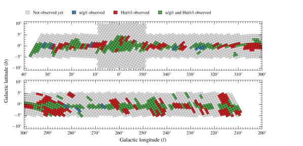
Figure 1: The VPHAS$+$ survey footprint plotted in Galactic coordinates. All 2269 fields are shown in outline. Different colours, as specified in the key, are used to identify the observations obtained for each field by 1st January 2014 – essentially 2 years after the start of data-taking.

Any comprehensive survey of the Galactic Plane clearly targets the main mass component of our own Galaxy, made up of stars, gas and dust. When a spatial resolution of 1 arcsec is combined with wide area coverage spanning 100s of square degrees, as in IPHAS, UVEX and VPHAS$+$, it becomes possible to exploit the stellar photometry adaptively to solve for the distribution of both the stars and dust making up the optically-accessible Galactic disk - by means that are similar to those already attempted, based on the near-infrared 2MASS survey (Drimmel & Spergel 2001, Marshall et al 2006). Methods to achieve 3-dimensional mapping of this kind, now incorporating the direct sensitivity of the H$\alpha$ narrowband to stellar intrinsic colour, are starting to take shape (Sale et al 2009; Sale 2012). This development coincides with the approach of the operations phase of Europe’s next major astrometric mission, Gaia. Indeed, the rich dynamical picture that Gaia will build of the Milky Way over the next decade will be very effectively complemented by stellar energy distributions measured for millions of stars from the current generation of ground-based optical, and near-infrared, wide-field surveys. VPHAS$+$, with its haul of photometry in 5 optical bands on $\sim$300 million objects, is set to take its place as one of them.

This paper presents the main features of VPHAS$+$, including a description of its execution, the data processing and the nature of the photometric colour information it provides. We begin in the next section with a presentation of the observing strategy and the data reduction techniques in use. We then turn to a description and evaluation of the narrowband H$\alpha$ filter procured for this survey, in section 3. Following this, in section 4, we present tailored synthetic photometry of main sequence and giant stars that provides insights into the photometric diagrams that may be generated from survey data. An exercise in photometric validation is described in Section 5 in which Sloan Digital Sky Survey (SDSS) data are compared with VST observations. The scene is then set for an example of VPHAS+ photometry extracted across the entire square-degree footprint of a single survey field (Section 6). In Sections 7 and 8, we outline the applications of VPHAS$+$ to spatially-resolved nebular astrophysics and in the time domain. The paper ends in Section 9 with a summary, examples of early survey exploitation, and a forward look to the first major data release.

2 Survey observations and data processing

2.1 VPHAS$+$ specification

The footprint of the survey is shown in figure 1. The OmegaCAM imager (Kuijken 2011) on the VST provides a field size of a full square degree, captured on a 4 x 8 CCD mosaic. After allowing for some modest overlap between adjacent fields, we arrived at a set of 2269 field centres that will cover the desired Galactic latitude band $-5^{\circ}<b<+5^{\circ}$ at all southern-hemisphere Galactic longitudes, as well as incorporate the Galactic Bulge extensions to $-10^{\circ}<b<+10^{\circ}$ near the Galactic Centre. The survey footprint extends across the celestial equator by a degree or two to achieve an overlap with the northern hemisphere surveys IPHAS and UVEX of $\sim$100 sq.deg. altogether. This is to create the opportunity for some direct photometric cross-calibration.

The target depth of the survey is to reach to at least $\sim$20th magnitude, at 10$\sigma$, in each of the Sloan $u$, $g$, $r$ and $i$ broadband filters and narrowband H$\alpha$. The bright limit consistent with this goal is typically 12–13th magnitude. Presently, all VPHAS+ photometric magnitudes are expressed in the Vega system. The original concept was to collect the data in all 5 bands contemporaneously, in order to build a uniform library of snapshot photometric spectral energy distributions for 200 million or more stars. Practical constraints have modified this to the extent that the blue filters ($u$, $g$) are observed separately from the reddest ($i$ and $H\alpha$), with the $r$ band serving as a linking reference that is observed both with $u$,$g$ and $i$,$H\alpha$. The aim is also to keep the spatial resolution close to 1 arcsecond. OmegaCAM and the Paranal site are well suited to this in that the camera pixel size is 0.21 arcsec, projected on sky, and the median seeing achieved is better than 1 arcsec (on occasion falling to as little as 0.6 arcsec).

As a means to obtaining better quality control, and to ensure that only a minimal fraction of the survey footprint is missed due to the pattern of gaps between the CCDs in the camera mosaic, every field is imaged at 2 or 3 offset pointings. This strategy has been carried over from IPHAS and UVEX in the northern hemisphere, and has the consequence that the majority of imaged objects will be detected twice some minutes apart. In the $r$ band, there will be two arbitrarily-separated epochs of data, with typically two detections at each of them (i.e. 4 altogether).

2.2 VPHAS$+$ observations

The VST is a service-observing facility, with all programmes queued for execution as and when the ambient conditions meet programme requirements. VPHAS+ survey field acquisition began on 28th December 2011. Normally the constraint set includes a seeing upper bound of 1.2 arcsec: this is only set at a lower, more stringent value for fields expected to present a particularly high density of sources (e.g. in the southern Bulge). In order that the seeing achieved in the $u$ band is not greatly different from that in $i$ at the opposite end of the optical range, it is advantageous to separate acquisition of blue data from red – hence a split between ’blue’ ($u$,$g$,$r$) and ’red’ ($H\alpha$,$r$,$i$) observing blocks has been implemented. This split also permits the use of different moon distance and phase constraints, such that blue data are obtained when the moon is less than half full at an angular separation of not less than 60 degrees, while the limits for red data are set at 0.7 moon illumination and a minimum angle of 50 degrees. Avoiding bright-moon conditions is important in order to limit the amount of moonlight mixed in with diffuse H$\alpha$ emission in the reduced images. No requirement has been placed on the time elapsing between acquisition of blue and red data. However, the more forgiving constraints on the acquisition of the latter has meant that these are typically executed sooner than the former, with the result that many more fields have red data already than have blue (see fig 1). In all cases, the final constraint is that the sky is required to be clear, if not necessarily fully photometric.

An impressive feature of the camera, OmegaCAM, is its potential to deliver remarkably undistorted point-source images all the way across the 1-degree field of view. To realise this, it is critical that the VST has an actively-controlled primary. The operational price for this, at the present time, is that image analysis and correction has to be carried out at every filter change or after longer slews. The overhead added by this is about 3 minutes. To reduce the impact of this, observations of sets of 3 neighbouring fields are scheduled together, so that image analysis need only take place every 15-30 minutes – not much more often than would be essential, in any case, to compensate for the telescope’s tracking movement. As a result, ’contemporaneous’ in the context of VPHAS+ data-taking means that all 3 blue, or red, filters are typically exposed within 40-50 minutes of each other (cf. IPHAS, where the more compact camera allows much faster operation, bringing this elapsed time down to under 10 minutes). However, the time difference between the blue and red observing blocks for a given field, i.e. the $u$/$g$/$r$ data collection and $H\alpha$/$r$/$i$ data collection, can be anything from a few hours to more than a year.

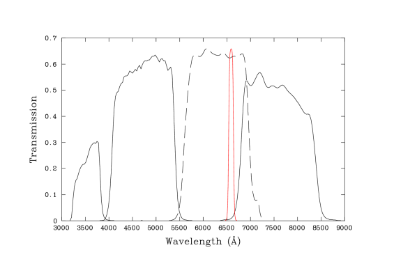
Figure 2: The transmission profiles of the Sloan $u$, $g$, $r$ and $i$, and narrowband $H\alpha$ filters used in all VPHAS$+$ observations. The $r$ and $H\alpha$ profiles are shown as a dashed line and in red respectively just to clearly distinguish them from each other and the $i$ band. Each profile has been multiplied by the CCD response function and a model of atmospheric throughput (Patat et al 2011). The very-nearly grey losses due to the telescope optics (a further scaling of approximately 0.6) have not been folded in.

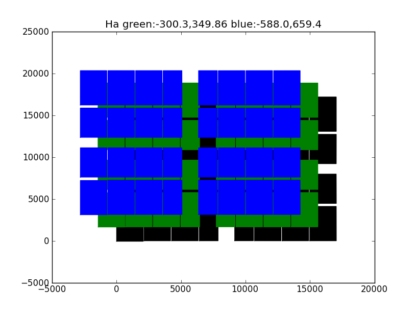
Figure 3: An illustration of the VPHAS$+$ offset pattern as it applies to the segmented H$\alpha$ filter with extra vignetting due to the T bars separating the 4 segments. The first pointing is to lower right, as drawn – a conservative estimate of the exposed unvignetted area is shown in black. The exposed/unvignetted areas of the second and third pointings are shown in green and blue respectively. The vertical and horzontal scales are numbered in pixels (RA increasing to the right, declination increasing upwards).

We provide a reminder of the passbands of the Sloan broadband filters in use, along with that of the narrowband H$\alpha$, in fig 2. They are shown scaled by a typical CCD response function and a model of the atmospheric transmission (Patat et al 2011). The exposure times used for the different filters, the number of exposures in each and the median seeing achieved, up to December 2013, are set out in Table 1. From early on, during the commissioning phase of the telescope, it became clear that tracking is usually good enough that even the 150 sec $u$ exposures, our longest, do not have to be guided in most circumstances. Indeed, experience is showing that it is safer to rely on the tracking, rather than the autoguider, to maintain good image quality in the most dense star fields.

Table 1: Observations obtained per survey field. The median seeing quoted is derived from data in hand by December 2013.

Filter	Exposure	No. of	median seeing
	time (secs)	offsets	(arcsec)
Blue observation blocks
$u$	150	2	1.01
$g$	40	3	0.88
$r$	25	2	0.80
Red observation blocks
$H\alpha$	120	3	0.84
$r$	25	2	0.82
$i$	25	2	0.77

The pattern of offsets used for each field is illustrated in fig 3. The shifts are relatively large, with the outer pointings differing by $-$588 arcsec in the RA direction and $+$660 arcsec in declination. The choices made have largely been driven by the characteristics of the narrowband H$\alpha$ filter (discussed below in section 3), but they also convey the advantage of greatly increasing the overlaps between neighbouring fields. Just the two outermost pointings are used when exposing the $u$, $r$ and $i$ filters. This leaves 0.4% of the survey footprint unexposed. This changes to complete coverage on including the third intermediate offset, as is the policy for the $H\alpha$ and $g$ filters.

In accordance with ESO’s standard procedures, data are evaluated soon after collection by Paranal staff and graded before transfer to the archive in Garching and to the Cambridge Astronomy Survey Unit (CASU) in Cambridge. If the applied constraints are significantly violated, the observation block is returned to the queue.

2.3 Data pipeline

2.3.1 Initial Processing

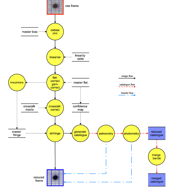
Figure 4: Flowchart identifying the main VST data processing steps. At the present time all steps up to the reduced single-band catalogue are undertaken at CASU. Band merging is performed at the University of Hertfordshire.

From February 29th 2012 raw VST data have been routinely transferred from Paranal to Garching over the Internet. For each observation the imaging data are stored in a Multi-Extension FITS file (MEF) with a primary header describing the overall characteristics of the observation (pointing, filter, exposure time, etc.) and thirty two image extensions, corresponding to each of the CCD detectors, with further detector-level information in the secondary headers. The 32-bit integer raw data files are Rice-compressed at source using lossless compression (e.g. Sabbey 1998). The files are then checked and ingested into the ESO raw data archive in Garching. As soon as the data for any given night become available they are automatically transferred to the Cambridge Astronomy Survey Unit (CASU) for further checks and subsequent processing. The VST web pages at CASU provide an external interface for both monitoring processing status (http://casu.ast.cam.ac.uk/vst/data-processing/) and overall survey progress and access (http://casu.ast.cam.ac.uk/vstsp/).

The processing sequence is similar to that used for the IPHAS survey of the northern Galactic Plane (e.g. Gonzalez-Solares et al 2008), while the higher level control software is based on that developed for the VISTA Data Flow System (VDFS, Irwin et al 2004). Here we briefly outline the processing steps illustrated in figure 4, emphasising the main differences relative to the current VDFS standard. A more detailed description of the VST processing pipeline is currently in preparation (Yoldas et al 2014).

Science images are first debiassed. Full two-dimensional bias removal is necessary due to amplifier glow during readout being present in some detectors. The master bias frames are updated daily from calibration files taken as part of the operational cycle. The OmegaCAM detectors are linear to better than 1% over their usable dynamic range removing the need for a linearity correction. Hence this stage in the pipeline processing (figure 4), although part of the pipeline architecture, is currently bypassed.

Flatfield images in each band are constructed by combining a series of twilight sky flats obtained in bright sky conditions. The timescale to obtain sequences of these for all deployed filters is typically one to two weeks. So as to adequately trace the variations in the pattern and level of scattered light in these flats, the master flats derived from them are updated on a monthly cycle (how these are corrected for scattered light is described in Section 2.3.3). Four of the detectors, in extensions 29–32, suffer from inter-detector cross-talk, whereby saturated bright stars in one detector can cause noticeable positive or negative low level ($\approx$0.1%) ghost objects in adjacent detectors. The impact of these is minimised in the pipeline by applying a pre-tabulated cross-talk correction matrix to each of the affected images.

The flatfield sequences plus bad pixel masks are used to generate the confidence (weight) maps (e.g. Irwin et al 2004) used later during catalogue generation and any subsequent image stacking or large area mosaicing. After flatfielding, science images generally have well behaved sky backgrounds which makes subsequent image processing straightforward. Where direct scattered light is present in them, it is an additive phenomenon that is dealt with automatically during object catalogue generation.

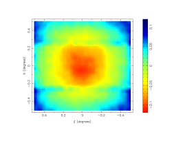
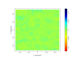
Figure 5: The left-hand panel shows an example of the deduced scattered light component present in June 2013 $r$-band data. The right-hand panel shows the corrected outcome. These maps were constructed using 286318 APASS object matches over the square-degree field. Before correction scattered light gradients amounting to a 20 to 25 percent variation from corners to centre are present. This flattens to around $\pm$2 percent.

The redder passbands used in VST observations, in this case the $i$-band, show fringing patterns at $\approx$2% of the sky background level. Defringing is done using a standard CASU procedure (Irwin & Lewis 2001). The fringe frames used are derived from other VST public survey data taken as close as possible in time at higher Galactic latitude. This approach works because the fringe pattern induced by sky emission lines at Paranal is quite stable over long periods. The fringe frames are automatically scaled and subtracted from each science image reducing the residual fringing level to well below the sky noise.

Catalogue generation is based on IMCORE (Irwin, 1985) and makes direct use of the confidence maps, derived from the flat fields, to suitably weight down unreliable parts of the images. This step includes object detection, parameterization and morphological classification, together with generation of a range of quality control information. Because of the extensive presence of diffuse emission throughout the southern Galactic Plane, particularly in H$\alpha$, a version of each affected image is cleaned of nebulosity using the NEBULISER for the purpose of catalogue generation only. This achieves a more careful removal of background and ultimately leads to more complete and, on average, more faithful object detection than in the absence of this step.

With object catalogues available for every VPHAS+ survey image, it is then possible to improve the rough World Coordinate System (WCS) based on the telescope pointing and general system characteristics. The WCS is progressively refined using matches between detected objects and the 2MASS catalogue (Skrutskie et al 2006). Despite the large field of view, the VST focal plane is almost free of distortion, and a standard tangent plane projection yields residual systematics of $\sim$25mas over the entire field.

2.3.2 Photometric Calibration

Provisional photometric calibration is based on a series of standard star fields observed each night (e.g. Landolt 1992). For each night a zeropoint and error estimate using the observations of all the standard fields in each filter is derived. The flatfielding stage nominally places all detectors on a common internal gain system implying, in principle, that a single zeropoint suffices to characterise the whole focal surface. Colour equations are used to transform between the passbands in use on the VST and the Johnson-Cousins system of the published standard-star photometry. The calibration is currently in a VST system that uses the SED of Vega as the zero-colour, almost zero-magnitude, reference object.

The $u$ band data are the most challenging to calibrate. As this part of Vega’s spectrum, and also the average standard star plus the detector reponse, are falling rapidly it would be surprising if there were no offsets in $u$ due to nonlinearities in the required colour transforms and, perhaps, to degenerate colour transforms for hotter stars. Early experience of working with $u$ data do indeed suggest that offsets of up to a few tenths of a magnitude are sometimes present (see Sections 5 and 6).

The colour transforms currently in use to define the VPHAS internal system are given below.

$$u_{VST} = U+0.035\,(U-B)$$

$$g_{VST} = B-0.405\,(B-V)$$

$$r_{VST} = R+0.255\,(V-R)$$

$$i_{VST} = I+0.215\,(R-I)$$

$$H\alpha_{\,VST} = R+0.025\,(V-R)$$

The transform for the narrowband H$\alpha$ is an approximate initial solution needed for the subsequent illumination correction stage. At catalogue bandmerging this is superceded (see Section 4).

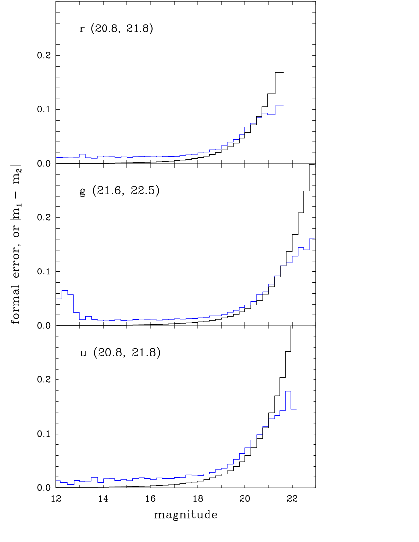
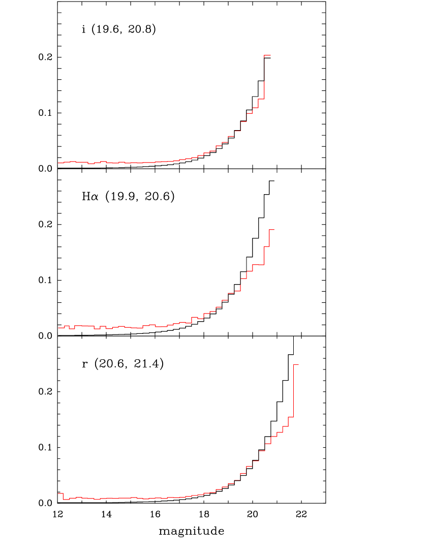
Figure 6: Photometric errors in VPHAS$+$ data as a function of magnitude. All data are drawn from an area of $\sim$0.2 sq.deg in field 1679, positioned $\sim$20 arcmin E of Westerlund 2. The left hand panel refers to blue observing block (OB) data, while the right refers to red OB data. The coloured histogram in each component plot shows the mean absolute deviation of the magnitude difference, $(m_{1}-m_{2})$, per 0.25-magnitude bin, while the bin means of the suitably-corrected pipeline estimate of the random error on this difference are in black. The 10- and 5-$\sigma$ magnitude limits are specified in the brackets next to each filter name. The rising observed mean deviation seen in $g$ at the bright end is due to the onset of saturation.

2.3.3 Illumination Correction

The main difficulty in deriving an accurate photometric calibration over the one degree field arises from the multiplicative systematics caused by scattered light in the flatfields. The VST (at least up to the introduction of baffles early in 2014) has proved particularly susceptible to variable scattered light. Its impact has varied from month to month depending on conditions prevalent at the time the flat-field sequences were taken. An illustration of the amount and character of the master-flat correction required is provided in figure 5.

The scattered light is made up of multiple components with different symmetries and scales. These range from $\approx$10 arcsec with x-y rectangular symmetry, e.g. due to scattering off masking strips above the CCD readout edges, to large fractions of the field due to radial concentration of light in the optics and to non-astronomical scattered light entering obliquely in flatfield frames. After some experimentation, and external verification, we found that the APASS all-sky photometric g,r,i catalogues (http://www.aavso.org/apass) provide a reliable working solution to the illumination correction problem inherent in VST data (see fig 5). These catalogues also provide an independent overall photometric calibration tied to the SDSS AB magnitude system and will be used in future updates to define an alternative finer-grained temporal AB magnitude zeropoint.

All filters used are treated in the same manner with colour equations set up to define transformations between the APASS g,r,i SDSS-like calibration and the VPHAS+ u,g,r,i,H_α internal system.

Illumination corrections are re-derived for each filter once a month. Application of these corrections via the master flats reduces the residual systematics across the entire field to below the 1% level for the broadband filters and to within 2% for the segmented narrowband H$\alpha$, except in vignetted regions (see Section 3).

2.3.4 Quality Control

In addition to the usual VDFS quality-control monitoring of average stellar seeing and ellipticity, sky surface brightness and noise properties, we have also initiated a more detailed analysis of the image properties based on inter-detector comparisons.

The well-aligned coplanar detector array coupled with the curved focal surface is extremely sensitive to imperfections in focus which are relatively easy to detect using the detector-level average seeing measurement variation available for each of the 32 detectors. Likewise the variation in average stellar ellipticity from each detector over the field is used to monitor rotator angle tracking problems.

All of this information can be used in addition to the observation block (OB) grades provided by ESO and is incorporated within all data product files and also the progress database.

2.4 Limiting magnitudes and errors

The present convention for VPHAS+ and this paper is that all magnitudes are expressed in the Vega system, which imposes zero intrinisc colour for A0 stars. The 5-sigma limiting magnitudes commonly achieved per exposure range from 20.5–21.0 for H$\alpha$ up to 22.2–22.7 for Sloan $g$. The 10$\sigma$ limits are about 1 magnitude brighter.

Every source flux or magnitude determined via the pipeline has a formal error associated with it. We provide an example of how these compare with empirical magnitude differences, by extracting a sample of stars from a 0.25 sq.deg catalogue, cut out from the survey field including Westerlund 2 (field 1679, see also sec 6) in order to examine the pattern of errors (fig 6). The sky area chosen is offset from the cluster to the east by $\sim$20 arcmin and exhibits moderate diffuse ionised nebulosity. In the southern Plane, the presence of some nebulosity, particularly affecting $r$ and $H\alpha$ exposures, is more the rule than the exception. Sources classified as probable stars in both $g$ and $r$ (blue filter set, left panel) and $r$ and $i$ (red filter set, right hand panel) in two consecutive offset exposures have been selected. The selection also required that each extracted magnitude was unaffected by vignetting and bad pixels (confidence level $>95$). This step is particularly important for H$\alpha$ given the extra vignetting introduced by the cross bars of the segmented filter (see Section 3).

The faintest stars that might have been included in the plots for $i$ and blue $r$ (top row in fig 6) are absent because of a requirement that every included source should also be picked up in, respectively, red $r$ and $g$. Fainter objects than the apparent limits certainly exist in these bands. This feature follows directly from the typically red colours of Galactic Plane stars at magnitudes fainter than $\sim$13 that are the target of this survey. For the same reason, it is not uncommon for the $u$ band source counts to be one or more orders of magnitude lower than those of the $i$ band. The role of the $u$ band is to pick out the unusual rather than to characterise the routine.

To bring out the systematic effects present, the specific comparison made in fig 6 is between the bin means of the absolute magnitude differences, $|m_{1}-m_{2}-\delta|$, between the two exposures, and the expected random error on the difference derived from the pipeline rms errors on the individual magnitude measurements. The quantity, $\delta$, is the median magnitude difference computed from all bright stars down to 18th magnitude ($r$, $i$ and H$\alpha$), or 19th magnitude ($u$ and $g$). This was small in all cases – the largest value being 0.011 for $u$. On the other hand, the correction applied to the pipeline errors was, first, to multiply the single-measurement magnitude error by $\sqrt{2}$ to give the rms error on the $(m_{1}-m_{2})$ difference, and then to multiply by $\sqrt{2/\pi}$ in order to convert the measure of dispersion from rms to a mean deviation.

At magnitudes brighter than 18–19 in fig 6, the scatter in the empirical results can be seen to be appreciably greater than that ’predicted’ for the random component by the pipeline. The scale of the difference indicates that a further error component of $\sim$0.01–0.02 magnitudes is present. The amount and filter-dependence of these levels of error are entirely consistent with the uncertainties estimated above for the flatfield and illumination corrections: as noted in section 2.3.3, the VST is presently prone to quite high and variable levels of scattered light. Practical remedies for this are under consideration by ESO – when implemented these should tighten up the error budget.

The enhanced mean magnitude difference seen for $g<13$ in fig 6 is typical of what is seen as saturation effects begin to set in. For all the other bands, in this example, saturation sets in at magnitudes a little brighter than 12th. A safe working assumption across VPHAS+ would be that saturation is never troublesome at magnitudes fainter than 13, but always an issue for magnitudes brighter than 12.

Figure 6 identifies the 5$\sigma$ and 10$\sigma$ magnitude limits for each filter achieved in this representative example. The seeing at the time of these observations, as measured in the pipeline, ranged from 0.8 to 1 arcsec (cf Table 1).

3 The narrowband $H\alpha$ filter

3.1 Overview

Table 2: Summary of filter segment properties

Segment	sky quadrant	CCDs covered	centre, mean, corner CWL	mean integrated
			(Å)	throughput (Å)
A	SW	1 – 8	6580.2 – 6585.4 – 6595.3	98.64
B	SE	17 – 24	6596.1 – 6585.4 – 6578.9	103.38
C	NE	25 – 32	6582.8 – 6591.9 – 6599.8	99.74
D	NW	9 – 16	6581.7 – 6594.3 – 6603.8	99.49

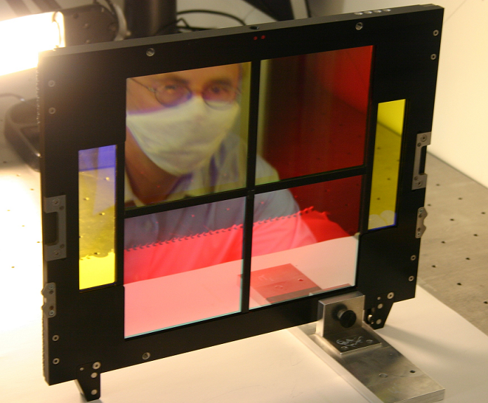
Figure 7: The segmented H$\alpha$ filter, photographed in the lab soon after receipt and just prior to measuring its transmission. The filters to either side of the 2$\times$2 array of H$\alpha$ segments, transmit as $r$-band and cover the guide CCDs.

A filter required to select a narrow band across a large 27$\times$27 cm² image plane is a challenging fabrication problem. At the telescope, the filter in use for VPHAS$+$ is known as NB-659. At the time it was commissioned in 2006, the purchase of a single-piece narrowband filter was offered only by one supplier and was well beyond budget. This left the 4-segment option as the achievable alternative.

The H$\alpha$ filter was constructed based on a specification supplied by the OmegaCAM consortium, setting as goal a central wavelength of 6588 Å, and a bandpass of 107 Å. It was delivered in the summer of 2009, and was shortly thereafter tested at the University of Munich Observatory, using the optical lab set up by the OmegaCAM consortium for filter testing. A photo of the filter at that time is shown in figure 7. The transmission of each filter segment was measured at 21 positions forming a coarse radial pattern (fig 8) using a monochromator beam adjusted to emulate the f-ratio 5.5 VST/OmegaCAM optical system. The logic of the chosen measurement pattern is to give a good sampling of the dominantly radial variation ofthe transmission profile due to the turntable rotation in the filter coating chamber. The diameter of the monochromator beam used in the measurements was 4-5 mm. This is a more compact beam than that of starlight at the telescope, which fills a spotsize of up to 12 mm on passing through the filter out of focus. Consequently, the actual performance will be a somewhat areally-smoothed version of the performance revealed by the lab measurements and their subsequent simulation. The filter was shipped to Paranal and VST in the spring of 2011, after some final selective remeasuring. These confirmed there had been no discernible bandpass changes in store since delivery almost 2 years earlier.

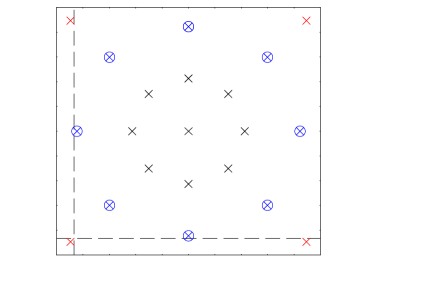
Figure 8: A map of the positions within each filter segment at which the transmission was measured. The colour codings are used again in later figures to distinguish the central positions (black, crosses, sampling roughly 30% of the segment area), intermediate radii (blue, encircled crosses, sampling $\sim$half the area), and corners (red crosses, 15% of the area – of which almost half is lost to vignetting). The dashed lines define the limits of the strips 2 arcmin wide that experience any vignetting due to the filter T-bars. They are drawn here as for segment D.

At the time the monochromator measurements were made, a segment naming scheme was put in place (segments A, B, C and D) which is re-used here. Presently the filter is housed in magazine B of OmegaCAM, which means that in terms of the view of the sky, segment A spans the SW section of the image plane, B the SE, while C and D span the NE and NW respectively. Table 2 identifies the mosaic CCDs beneath each segment, and sets down the centre-to-corner range in central wavelength (CWL) and the typical throughput integral. The laboratory tests showed us that the CWL of segments A, C and D is shortest in the segment centre, and drifts longwards according to a centro-symmetric pattern, as the corners and sides are approached. For segment B, the centre-to-corner drift is reversed, with the result that the corner CWLs are bluer than in the centre of the glass. Segment B also has the highest mean FWHM, and highest average peak transmission: integrated over the bandpass this is a difference in throughput of 0.045 magnitudes relative to A, C and D. The pipeline-applied illumination correction aims to eliminate this contrast. Area-weighted transmission profiles for the 4 segments are shown in fig 9, along with the overall mean profile. The latter is also given numerically in table 3.

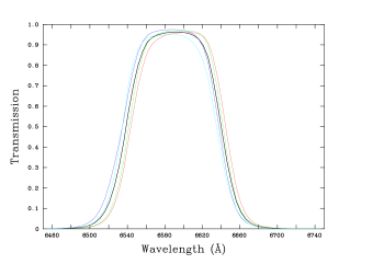
Figure 9: The mean transmission profiles of the individual glass segments, A to D (cyan, blue, green and red respectively), making up the $H\alpha$ filter and the overall mean profile (black).

Table 3: Mean transmission for NB-659

Wavelength	Transmission	Wavelength	Transmission
(Å)		(Å)
6456.3	0.000	6591.5	0.962
6461.3	0.001	6696.5	0.961
6465.8	0.001	6601.0	0.960
6470.8	0.002	6616.0	0.955
6475.9	0.002	6611.0	0.945
6480.9	0.003	6616.1	0.928
6485.9	0.005	6621.1	0.896
6490.9	0.008	6626.1	0.839
6496.0	0.012	6631.1	0.736
6501.0	0.020	6636.2	0.609
6506.0	0.033	6641.2	0.466
6511.1	0.053	6646.2	0.230
6516.1	0.086	6651.2	0.219
6521.1	0.136	6656.3	0.133
6526.1	0.208	6661.3	0.081
6531.2	0.307	6666.3	0.048
6536.2	0.429	6671.3	0.029
6541.2	0.575	6676.4	0.018
6546.3	0.700	6681.4	0.011
6551.3	0.799	6686.4	0.007
6556.3	0.868	6691.5	0.005
6561.4	0.915	6696.5	0.003
6566.4	0.936	6701.5	0.002
6571.4	0.947	6706.5	0.002
6576.4	0.954	6711.5	0.001
6581.5	0.959	6716.5	0.001
6586.5	0.961	6721.6	0.000

Compared to the H$\alpha$ filter used in the IPHAS survey, NB-659 has a CWL that is redder on average by $\sim 20$ Å, it is around 10 percent wider, and has a higher overall throughput leading to zeropoints $\sim$0.2 higher. The known variations of bandpass across the 4 segments has implications for how best to exploit VPHAS+ data. To anticipate these we have carried out two types of simulation based on the lab measurements in order to identify them. We describe these next, and summarise the implications in Section 3.4.

3.2 Simulation of the main stellar locus in the $(r-H\alpha,r-i)$ diagram

To gain an impression of the extent of the uniformity of performance with regard to normal main sequence stars, ($r-H\alpha,r-i$) tracks were (1) computed for each measured $H\alpha$ transmission profile using exactly the same method as was followed by Drew et al (2005) for the analysis of IPHAS data, (2) rescaled to a common integrated throughput, mimicking the effect of the pipeline illumination correction, (3) compared to the mean pattern by subtracting off the computed mean track. The result of this is shown as fig 10. The track differences picked out in red are from the segment corners exhibiting the largest CWL shifts. It can be seen that the tracks follow the same trend to within $\pm$0.02 up to about $r-i=1.2$ (corresponding to M3 spectral type), after which there is a clear fanning out. This shows that the obtained $r-H\alpha$ excesses should fall within the target photometric precision range of the survey for all except mid- to late-M stars.

The sensitivity of the M stars to variations in the narrowband transmission profile is a point of note, while not actually a surprise. It arises from the great breadth of the feature in M-star spectra created by the absorbing TiO bands displaced to either side of the narrow H$\alpha$ bandpass, and the fact that the resulting inter-band flux maximum falls at wavelengths shortward of H$\alpha$. As these molecular bands strengthen with increasingly late spectral type, the $r-H\alpha$ apparent excess grows along with the sensitivity to the exact placement of the bandpass. Viewed in these terms, the $(r-H\alpha,r-i)$ colours of unreddened mid- to late-M dwarfs provide an empirical gauge of filter bandpass uniformity and/or typical CWL. To minimise the bandpass sensitivity and hence spread seen at late M, the CWL would need to be lowered to around 6530 Å or less. In practice, later M dwarfs are sufficiently faint that they normally appear in $(r-H\alpha,r-i)$ diagrams as a relatively sparse distribution of scarcely reddened objects – falling within a thinly-populated, continuation of the unreddened main sequence, redward of $(r-i)=1.0$, rising from $r-H\alpha\sim 0.5$ up to $\sim 0.8$, (see figs 17, or 20). Reddened M dwarfs are usually just too faint to be detected.

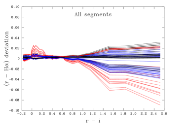
Figure 10: The r - H$\alpha$ deviations computed for all measured positions on the H$\alpha$ filter, NB-659, after correcting the data for bandpass integrated throughput variations. The data are colour-coded according to position of measurement as in fig 8. The most discrepant corner positions, all plotted in red, are located in segments C and D.

Selection of mid-to-late M dwarfs is therefore straightforward, but quantitative interpretation of $(r-H\alpha)$ should be presumed more uncertain than at earlier spectral types. Similar effects will be seen in the M-giant spur located at lower $(r-H\alpha)$ in the $(r-H\alpha,r-i)$ diagram (see fig 16). However, as red giants will be picked up by VPHAS+ at large distances through significant reddening, a precautionary check on the impact of non-zero extinction on this fanning in colour has been made: tracks of the type compared in fig 10 were recalculated for $A_{V}=6$ and no noticeable additional effect was found (see also fig 17).

3.3 Simulation of the impact of source radial velocity on in-band emission line fluxes

Simulations have also been performed to consider how the filter captures emitted $H\alpha$ flux, as a function of location within the field of view and source radial velocity. An ideal filter, centred on the mean rest wavelength of the imaged $H\alpha$ emission and placed in a high f-ratio optical path, would be insensitive to radial velocity shifts up to a limit proportional to the FWHM of the bandpass. The desired capabilities of the VPHAS+ H$\alpha$ filter are separation between H$\alpha$ emission line objects and the main stellar locus – and, better still, a regular mapping of measured $r-H\alpha$ excess onto emission equivalent width (cf Drew et al 2005, figure 6). The two representative spectra used to investigate how these capabilities are affected by changing source radial velocity are shown in fig 11.

Figure 11: Top panel: an example of a very bright, simple H$\alpha$ emission profile (taken from Corradi et al 2010). The emission equivalent width is 220 Å, and the FWHM of the observed profile is close to 390 km s^-1. The mean radial velocity of the line is $+$35 km s^-1. The difference between a pure continuum magnitude and that including the line is somewhat in excess of 1.2. Lower panel: the contrast of the line relative to continuum is much less here (EW $\sim$ 20 Å), and the FWHM is somewhat wider at 570 km s^-1 (a classical Be star, taken from Raddi et al, 2013). The mean radial velocity is $-$50 km s^-1. The continuum-only magnitude is fainter by about 0.2 only, here.

Both spectra were blueshifted to $-$500 km s^-1 , and then shifted redward in steps of 100 km s^-1 at a time, up to $+$500 km s^-1 (altogether a displacement of 22 Å) – calculating at each step the integral of the spectrum folded through the filter transmission profile. The resultant in-band fluxes were converted to magnitudes, and then shifted by the amount required to match the integrated transmission to the overall mean for the filter (again mimicking the function of the pipeline illumination correction). In real use, we would expect the majority of emission line objects to present with FWHM no greater than either of these examples (interacting binaries and WR stars do present with much broader emission, however).

The radial velocity range explored was chosen with the following considerations in mind:- Emission line stars in the thin disk will commonly have radial velocities falling within the range -100 to +100 km/s. In the Bulge larger radial velocities may be encountered: excursions to $\pm$200 km s^-1 are observed in CO (Dame, Hartmann & Thaddeus 2001) within $\sim 20^{\circ}$ of longitude of the Galactic Centre, and for a minority of inner-Galaxy planetary nebulae, radial velocities have been obtained that extend the range almost to $\pm$300 km s^-1 (see Durand, Acker & Zilstra 1998, and Beaulieu et al 2000).

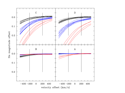
Figure 12: Results of simulation of the in-band flux as a function of source radial velocity for the EW = 220 Å emission spectrum (upper panel in fig 11). The fluxes are expressed as magnitude offsets relative to the peak simulated in-band flux. The panels representing the segments are arranged as they are imposed on the plane of the sky, i.e. A covers the SW quadrant, D covers the NW when the filter is stored in OmegaCAM’s magazine B. The curves are colour-coded according to measurement position as in fig 8. Galactic sources will usually fall well within the marked velocity range, $-$200 to $+$200 km s^-1. The more problematic red curves, representing the response of the segment corners, account for $\sim$8% of each segment’s unvignetted area only.

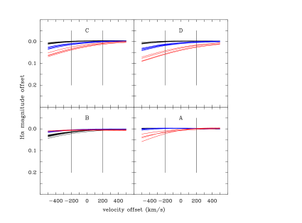
Figure 13: Results for an emission line net equivalent width of 20 Angstroms (spectrum shown in lower panel in fig 11). Otherwise as fig 12.

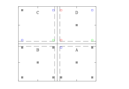
Figure 14: The layout of the H$\alpha$ filter, showing the positions of the PN-test measurements, colour coded according to flux relative to the corners of segment B. Those shown as black crossed boxes have a scaled flux $\geq 0.95$. Those in blue are a little lower with a scaled flux in the range 0.90 – 0.94. The two positions marked in green have fluxes scaling to 0.88 and 0.89, while the two in red scale to 0.84 and 0.77 (both in segment D). There is no measurement for the centre of segment C because of a telescope pointing imprecision. The other centre measurements were obtained $\sim 2$ arcmins away from the true centres plotted in order to avoid CCD gaps. The dashed lines mark the limits of the T-bar vignetting.

The results of this exercise are plotted in figs 12 and 13. Fig 12 shows that segments A and B come very much closer to independence of radial velocity than segments C and D, in terms of measured $H\alpha$ excess. In all segments, reasonable fidelity (a flat, or nearly flat response) is achieved around segment centre – although in B, uniquely, the corners happen to perform a little better than the centre. Clearly segment D, where the transmission is centred on longer wavelengths than in the other segments, could yield measurements in its corners (perhaps 8% of its unvignetted area) of $H\alpha$ magnitude, or of $r-H\alpha$, that underestimate the flux of similarly high equivalent-width H$\alpha$ emission by up to $\sim$ 0.3 (out of a true excess, expressed in magnitudes of $\sim 1.2$). Segment C performs similarly, but the potential flux drop associated with its corners is less pronounced.

We can compare the expectations created by these simulations with the results of an on-sky experiment in which the planetary nebula (PN) ESO 178-5 (or PNG 327.1 -02.2) has been exposed in H$\alpha$ at a series of positions in the image plane, placing it well into every corner and also close to the centre of each of the four filter segments (see fig 14). The observed integrated counts variation might be predicted to be somewhat stronger than in fig 12 given that the in-band continuum flux from this PN will be relatively even weaker. But this will be offset by the additional flux due, in particular, to [NII] $\lambda$6584. The PN chosen for this test was picked both because it is well-calibrated (Dopita & Hua 1997), and because its LSR radial velocity is quite large and negative ($v_{LSR}=-88.7$ km s^-1: on 19th April 2013 when it was observed, this will have shifted to $-105$ km s^-1 at the telescope). It also happens to possess [NII] $\lambda$6584 emission that is scarcely less bright than H$\alpha$ (the former has 98% the flux of the latter: Dopita & Hua also provide a spectrum of this nebula).

Background-subtracted aperture photometry of the PN and a moderately bright star nearby, serving as a continuum reference, was carried out on the reduced images. These measurements reveal a pattern of behaviour that essentially tracks the results shown in figure 12: the continuum reference itself shows a total count variation of $\pm 5$% across all pointings, while the PN counts, after scaling to the reference, range from $+5$%, down to $-23$% relative to the values for the corners of segment B. In the extreme case that all of the H$\alpha$ and [NII] $\lambda$6548 emission had been shifted out of the bandpass, the maximum drop for this PN would be $-57$% (the remaining 43% being attributable to [NII] $\lambda$6584). The pattern across the filter of the results emerging from this trial is shown in fig 14.

The radial-velocity dependence of the transmitted flux may accordingly become an issue for objects with very strong H$\alpha$ emission where the aim is accurate flux determination, unless attention is paid to where the object falls in the image plane. Qualitatively the issue is less critical: regardless of where the object is located, the changes in transmission are not so large that there will be frequent failures to distinguish strong H$\alpha$ emitters – i.e. they will still appear above the main stellar locus in the $(r-H\alpha,r-i)$ diagram. In the example simulated, the outer reaches of segment D would bring $(r-H\alpha)$ down to 0.9 – 1.0, a level that nevertheless remains clear of the domain that might be occupied by unreddened, non-emission very late-type M dwarfs ($(r-H\alpha)\sim 0.8)$, cf fig 16). As further context, we note that nearly continuum-free emission line objects, such as PNe and HII regions, present with $r-H\alpha\sim 3$.

Where the line emission itself contributes only a minority of the measured narrowband $H\alpha$ flux the trends seen are much more subdued (fig 13). For the example shown, only 20 percent of the total in-band flux is attributable to the net line emission, rather than most of it as in fig 12. Again, the corners of segments C and D perform least well, in under-representing the emission flux by up to $\sim$0.05 magnitudes at the most negative likely Galactic Plane radial velocities. Otherwise, the performance is predicted to be within the anticipated 0.02–0.03 error budget of the survey.

3.4 Implications of the H$\alpha$ filter properties for VPHAS+ and its exploitation

In summary, for most purposes the H$\alpha$ filter performs as required, and has very good throughput. For the great majority of stars making up the main stellar locus, there will be the desired fidelity of $(r-H\alpha)$ colour, and the great majority of emission line objects will be detected with the same facility as they are by IPHAS.

There are two caveats to note. First, in Section 3.2 it was shown that variations in central wavelength across the filter segments will lead to thickening of the loci traced by mid-to-late M stars. These same variations, of what is a relatively red H$\alpha$ passband, also introduce the potential for under-determination of H$\alpha$ fluxes for objects/nebulosity in parts of the image plane for sources with significantly negative radial velocities (Section 3.3). This becomes most serious for emission-line sources falling near the vignetted corners of segments D and C, where a $20-30$ percent under-counting in H$\alpha$ may occur for radial velocities approaching $-200$ km s^-1. As is always the case for narrowband H$\alpha$ filters, the common presence of significant [NII] $\lambda\lambda$6548, 6584 emission bracketing H$\alpha$ in planetary nebulae or HII regions complicates the expected signature. However, it can be guaranteed in all but rare, exotic circumstances that the stronger $\lambda$6584 component of the [NII] doublet falls well within the bandpass.

The outstanding practical consequence of the filter’s transmission characteristics for the survey strategy are that, for quantitative reliability, measures of $(r-H\alpha)$ obtained using segments A and B, and the central zones of C and D (out to $\sim 13$ arcmin) are to be favoured. This appreciation is half of the reason for the adoption of offsets of several arcminutes between the 3 successive pointings made in this filter (fig 3) for each field – our strategy ensures that objects captured in segment corners in the first pointing are fall close to segment centres in the third.

The rest of the motive is to mitigate the cross-shaped vignetting due to the blackened T-bars holding the segments in place (fig 7). Each arm of the cross casts a shadow entirely contained within a strip 4 arcmin wide. By choosing to offset at least this much in both RA and Dec between the 3 exposures obtained per field, we raise the probability of at least one high-confidence $r-H\alpha$ colour measurement per detected source in the final catalogue to very nearly 100 percent, and the probability of two to over 95 percent.

Finally, we remark that the combination of large offsets and three pointings has the consequence that the fraction of sky within the survey footprint missed altogether, due to dead areas between the CCDs and vignetting, is under 0.3 percent.

4 Simulation of VPHAS$+$ stellar colours

The five bandpasses of the survey provide the basis for the construction of a range of magnitude-colour and colour-colour diagrams. To take full advantage of them, knowledge is needed of the behaviours that can be expected of the colours of normal stars.

We have simulated colours for solar-metallicity main sequence and giant stars using the same method as employed by Sale et al. (2009). We adopt the definition of these two sequences in $(T_{eff},\log g)$ space given by Straizys & Kuriliene (1981). Then for each spectral type along these sequences, solar-metallicity model spectra were drawn from the Munari et al. (2005) library. At a binning of 1 Å  the spectra in this library are well enough sampled to permit the calculation of narrow-band $H\alpha$ relative magnitudes with confidence, alongside the analogous broadband quantities. More detail on the broadband filter transmission profiles, shown in Fig. 2, and on the CCD response curve is provided on the ESO website. To ensure compliance with the Vega-based zero magnitude scale, we have defined the synthetic colour arising from a flux distribution $F_{\lambda}$ as follows:

$$m_{1}-m_{2}=-2.5\log\left[\frac{\int T_{1}\lambda F_{\lambda}d\lambda}{\int T_{1}\lambda F_{\lambda,V}d\lambda}\right]+2.5\log\left[\frac{\int T_{2}\lambda F_{\lambda}d\lambda}{\int T_{2}\lambda F_{\lambda,V}d\lambda}\right]$$

where $T_{1}$ and $T_{2}$ are the numerical transmission profiles for filters $1$ and $2$, after multiplying them through by the atmospheric transmission (Patat et al 2011) and mean OmegaCAM CCD response curves. The SED adopted for Vega, $F_{\lambda,V}$, is that due to Kurucz (http://kurucz.harvard.edu/stars.html). Where needed for comparison, we have also computed colours based on the Pickles (1998, hereafter P98) spectrophometric stellar library (the approach adopted by Drew et al 2005 for IPHAS). To maintain precision, the numerical quadrature resamples the more smoothly varying transmission data onto the sampling interval of the stellar SED.

The $(r-H\alpha)$ excess is evaluated in exactly the same way as the broadband colours. Since Vega is an A0V star, its SED at H$\alpha$ incorporates a strong absorption line feature that reduces the in-band flux below the pure continuum value. Unlike the broadbands, the $H\alpha$ narrowband has not yet been standardised and so there is not a formally recognised flux scale. However, we can specify here that the integrated in-band energy flux for Vega, on adopting the mean profile for the VST filter, is $1.84\times 10^{-7}$ ergs cm^-2 s^-1 (at the top of the Earth’s atmosphere). To assure zero colour relative to the optical broad bands, this flux is required to correspond to $m_{H\alpha}\simeq 0.03$. The reduction in zeropoint (zpt) that the computed in-band flux implies relative to the flux captured by the much broader $r$ band – based on folding Vega’s SED with lab measurements of the filter throughputs corrected for atmosphere and detector quantum efficiency – is 3.01. Current practice in VPHAS+ photometric calibration is accordingly to adopt zpt(NB-659) = zpt(r) - 3.01 magnitudes as the default calibration for the narrowband: in section 5 where a direct comparison is made with SDSS spectroscopy, this offset is found to be satisfactory. When applied, it assures that data obtained in photometric, or stable, conditions, yield zero $r-H\alpha$ colour for A0 stars.

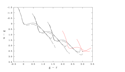
Figure 15: The expected positions of main sequence and giant stars in the $(u-g,g-r)$ plane. For the main sequence, tracks are shown for the monochromatic reddenings $A_{0}=$ 0, 2, 4, 6 and 8 (working from left to right). The red leak in the $u$ filter starts to lower $u-g$, noticeably from $A_{0}=6$ (tracks drawn in red). The giant-star tracks, drawn as dashed lines for $A_{0}=0$, 2 and 4 only, are very similar to their main-squence counterparts except at the latest types.

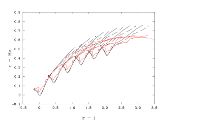
Figure 16: The expected position of main sequence and giant stars in the $(r-H\alpha,r-i)$ plane. Tracks are shown for the monochromatic reddenings $A_{0}=$ 0, 2, 4, 6, 8 and 10 (from left to right). Solid lines represent the main sequence tracks, while dashed lines are used for the giant tracks. The lines in red are giant-star tracks derived from P98 spectrophotometry.

Both main-sequence and giant-star colours have been calculated for a range of reddenings and optical-IR extinction laws as formulated by Fitzpatrick & Massa (2007). The unreddened colours for the mean Galactic law ($R=3.1$) are laid out here in table 4. The Appendix provides additional tables that specify the colours of main sequence stars at selected reddenings and for two further representative reddening laws ($R=2.5$ and 3.8). These can be used to construct intrinsic-colour-specific reddening lines. For the large range in extinction sampled along many Galactic Plane sightlines, these reddening trends are slightly curved (see the examples shown in e.g. Sale et al 2009). In this paper we use $A_{0}$, the monochromatic reddening at 5500 Å to parameterise the amount of reddening, rather than the band-averaged measure, $A_{V}$. In most circumstances these quantities are almost identical.

Table 4: VST/OmegaCAM synthetic colours for unreddened main-sequence dwarfs and giants.

Sp.type	main sequence (V)					giants (III)
						(model)				(P98 library spectra)
	$u-g$	$g-r$	$r-i$	$r-H\alpha$		$u-g$	$g-r$	$r-i$	$r-H\alpha$	$r-i$	$r-H\alpha$
O6	-1.494	-0.313	-0.145	0.071
O8	-1.463	-0.299	-0.152	0.055						-0.158	0.074
O9	-1.426	-0.271	-0.142	0.064		-1.426	-0.271	-0.142	0.064
B0	-1.404	-0.267	-0.143	0.058		-1.404	-0.267	-0.143	0.058
B1	-1.296	-0.236	-0.130	0.052		-1.316	-0.234	-0.130	0.057	-0.095	0.071
B2	-1.181	-0.214	-0.117	0.049		-1.209	-0.211	-0.116	0.056
B3	-1.025	-0.182	-0.098	0.048		-1.046	-0.182	-0.098	0.054	-0.035	0.083
B5	-0.799	-0.133	-0.071	0.043		-0.814	-0.134	-0.072	0.050	-0.016	0.083
B6	-0.699	-0.116	-0.062	0.040		-0.714	-0.116	-0.062	0.046
B7	-0.550	-0.094	-0.051	0.033		-0.568	-0.095	-0.051	0.041
B8	-0.361	-0.071	-0.039	0.022		-0.383	-0.072	-0.039	0.032
B9	-0.168	-0.040	-0.023	0.009		-0.186	-0.044	-0.024	0.021	-0.018	0.035
A0	-0.024	0.000	-0.003	-0.002		-0.030	-0.009	-0.006	0.011	0.012	0.034
A1	0.007	0.015	0.004	-0.004		0.007	0.004	0.000	0.008
A2	0.039	0.038	0.014	-0.005		0.051	0.022	0.009	0.008
A3	0.064	0.062	0.025	-0.005		0.085	0.045	0.019	0.007	0.037	0.063
A5	0.096	0.130	0.056	0.008		0.143	0.107	0.048	0.015	0.096	0.087
A7	0.073	0.206	0.089	0.030		0.145	0.179	0.078	0.032	0.115	0.094
F0	0.003	0.336	0.153	0.086		0.091	0.317	0.144	0.084	0.156	0.102
F2	-0.021	0.396	0.182	0.111		0.064	0.380	0.174	0.109	0.204	0.172
F5	-0.039	0.505	0.230	0.150		0.046	0.491	0.224	0.148	0.238	0.164
F8	-0.013	0.587	0.263	0.174
G0	0.012	0.628	0.278	0.185						0.333	0.213
G2	0.011	0.628	0.279	0.185		0.253	0.759	0.329	0.215
G5	0.162	0.756	0.327	0.217		0.405	0.870	0.368	0.235	0.396	0.250
G8	0.355	0.845	0.358	0.233		0.531	0.944	0.395	0.247	0.419	0.247
K0	0.523	0.938	0.396	0.248		0.640	1.002	0.417	0.256	0.446	0.254
K1	0.551	0.954	0.403	0.251		0.803	1.085	0.451	0.269	0.468	0.269
K2	0.629	0.993	0.419	0.258		0.963	1.159	0.483	0.281	0.508	0.293
K3	0.779	1.062	0.447	0.269		1.227	1.276	0.536	0.299	0.514	0.286
K4	0.871	1.108	0.468	0.278		1.374	1.342	0.585	0.320	0.592	0.313
K5	1.083	1.210	0.522	0.300		1.578	1.420	0.630	0.338	0.714	0.337
K7	1.387	1.402	0.724	0.387
M0	1.372	1.411	0.789	0.411		1.697	1.454	0.686	0.360	0.827	0.411
M1	1.335	1.439	0.934	0.467		1.838	1.506	0.769	0.395	0.872	0.401
M2	1.262	1.442	1.112	0.522		1.938	1.546	0.825	0.420	0.920	0.443
M3	1.236	1.447	1.179	0.545		1.980	1.556	0.933	0.444	1.165	0.471
M4	1.248	1.457	1.168	0.543		1.959	1.551	1.136	0.500	1.472	0.512
M5						2.009	1.569	1.296	0.556	1.739	0.560
M6						2.199	1.612	1.267	0.554

Based on the data from these tables, the main sequence and giant tracks are as shown in figures 15 and 16. These identify where the main stellar loci will fall. It is important to note that the OmegaCAM $u$ filter, like all filters constructed for this challenging band, exhibits a low-level red leak. In this instance, lab measurements indicate transmission at levels between $10^{-5}$ and $10^{-4}$ within limited windows around $\sim$9000 Å. This is enough to begin to noticeably, and erroneously, brighten the $u$ magnitudes of normal stars reddened to $g-r>3$. Because of this, and because the measurement of very low level leakage is itself subject to proportionately higher uncertainty, we do not plot or tabulate $u-g$ data beyond $g-r=3$ limit. Very few detected sources are so extreme. In practice, VPHAS+ $u-g$ is faithful for extinctions up to $A_{0}\sim 6$, but gradually thereafter it transforms into a colour that behaves crudely as $-(g-z)$.

The $(r-H\alpha,r-i)$ colour-colour diagram is not subject to such effects, and therefore remains sound across a wider spread in visual extinctions. Synthetic tracks are presented in figure 16 for $A_{0}=0$, 2, 4, 6, 8 and 10. The main sequence tracks shown are similar to those appropriate to IPHAS (cf figure 6 of Sale et al 2009). But a problem emerges when it comes to the simulation of red giant colours. Purely theoretical simulation predicts late-K and M giant colours closely resembling those of dwarfs, whereas simulation using P98 library spectrophotometry indicates a distinctive flattening of the M-giant track, peeling away from the steadily rising main sequence track. Figure 16 points out this contrast. Inspection of table 4 reveals this is a problem linked mainly to simulation of the $i$ spectral range, which renders $(r-i)$ progressively larger from late K into the M giant range when the library spectra are used in place of model atmospheres.

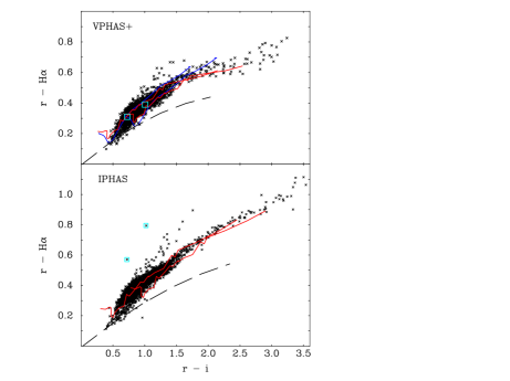
Figure 17: Equatorial VPHAS+ data (upper panel) and IPHAS data (lower panel) compared to show the different appearance of M-giant $(r-H\alpha,r-i)$ colours. The photometry is extracted from a $\sim$0.2 sq.deg region of sky, centred on $\ell=35.95^{\circ}$, $b=-3.13^{\circ}$. The magnitude range is limited to $13<r<18$ in both cases. Telescope-appropriate giant tracks, computed from the P98 spectrophotometric library, for $A_{0}=$ 2 and 4 are superimposed in red in both panels. In the upper panel, giant tracks computed from model atmospheres for the same reddenings are shown in blue. The black dashed line in each panel is the synthetic early-A reddening line, from $A_{0}=0$ to $A_{0}=10$. The stars appearing in the IPHAS catalogue as candidate emission line stars are enclosed in cyan boxes in both panels.

Evidence that M giants are better reproduced by synthetic photometry based on flux-calibrated spectra is provided by figure 17. This figure also compares new VPHAS+ data with their crossmatches in the IPHAS survey within a $\sim$0.2 sq.deg equatorial field ($\ell=35.95^{\circ}$, $b=-3.13^{\circ}$), and shows selected synthetic tracks superimposed. The photometry from the two surveys of the most densely populated part of the main stellar locus to $(r-i)\simeq 1.5$ substantially overlap, but not perfectly – the response functions describing the three bandpasses involved in fig 17 undoubtedly differ in detail between the two telescopes. On cross-correlating either $(r-i)$ or $(r-H\alpha)$ between the two surveys, it becomes clear that the IPHAS colour has the somewhat larger dynamic range. This is the reason for the slightly more stretched appearance of both the main locus and the early-A reddening line in the IPHAS diagram relative to that for VPHAS+.

At $(r-i)>1.5$ in fig 17, it can be seen that the M-giant spurs look very different. First, the VPHAS+ M giants fall into a nearly flat distribution lying at lower $(r-H\alpha)$, compared to the more steeply rising higher IPHAS M-giant sequence. However, as long as the data are interpreted with reference to telescope-appropriate synthetic photometry, the two datasets will lead to the same inference. In the example shown in fig 17, the comparisons with suitable synthetic giant tracks indicate that the maximal extinction in the field can be no more than $A_{0}\simeq 4$. The extinction measures due to Marshall et al (2006), based on 2MASS red-giant photometry, indicate a maximum Galactic extinction of $A_{K}\sim 0.3$ for this pointing. For a typical Galactic $R=3.1$ reddening law this scales up to $A_{0}\sim 3.3$ (roughly – see Fitzpatrick & Massa 2009). If model-atmosphere giant tracks are referred to instead, the M giants would have to be read as demanding visual extinctions ranging from $\sim$4 upwards.

Fig 17 also demonstrates the broadening in $(r-H\alpha)$ of the VPHAS+ M-giant sequence that was foretold in Section 3. The IPHAS counterpart is evidently much sharper, as it rises to higher $r-H\alpha$ with increasing $r-i$. The main practical impact of this difference is that IPHAS M-giant photometry is the better starting point for picking apart chemistry differences (Wright et al 2008). But it is as true of the VPHAS+ $(r-H\alpha,r-i)$ diagram as it is of its IPHAS equivalent – that M giants at $r-i>1.5$ sit below and apart from M dwarfs.

Fortuitously, fig 17 identifies an advantage of the generally good seeing available at the VST. There are two candidate emission line objects apparent in the IPHAS selection (enclosed in cyan boxes, in fig 17), that drop back into the main stellar locus in the VPHAS+ data. Inspection of the images shows that both stars are in close doubles of similar brightness, of under 2 arcsec separation. Because they are a little better resolved in VPHAS+ ($\sim$0.8 arcsec seeing), than in IPHAS ($\sim$0.9 arcsec seeing), the pipeline makes a better job of the assigning magnitudes in the different bands to the blend components. This example nicely illustrates the most common reason for bogus candidate emission line stars in either VPHAS+ or IPHAS - improperly disentangled blends. Candidate emission line stars should always be checked for this kind of problem before spectroscopic follow-up. Otherwise, experience with IPHAS gives confidence that the selection of emission line objects via VPHAS+ will be highly efficient (see e.g. Vink et al 2008, Raddi et al 2013).

Finally, it is worth noting that the bright limit of the survey at 12–13th magnitude effectively excludes any unreddened stars of earlier spectral type than $\sim$G0. Before more luminous stars of spectral type F and earlier can enter the survey sensitivity range, they need to be at distances in excess of 1 kpc, typically, where low extinction becomes increasingly improbable. This constraint bestows a significant selection benefit in that only unreddened or lightly-reddened subluminous objects, with intrinsically blue colours are left standing clear near the blue end of the main stellar locus in commonly-constructed photometric diagrams. In this domain VPHAS+ has important selection work to do.

5 Photometry validation: a comparison of SDSS and VST data

Before the start of survey field acquisition, we obtained observations in all survey filters of two pointings that fall within the SDSS photometric and spectroscopic coverage (Abazajian et al 2009). These were centred on RA 20:47:53.7 Dec -06:04:14.5 (J2000) and RA 21:04:25.94 Dec +00:59:15.8 (J2000) – fields that happen to include a number of white dwarfs and cataclysmic variables (not discussed further here). The main aim of the data was to verify VST photometry both by comparison to SDSS photometry and to synthetic photometry derived from SDSS spectra. The VST observations were obtained on 21/09/2011, during clear weather at a time of generally sub-arcsecond seeing. The exposure times differ only a little from those now in general survey use: the $g$ exposures were 30 sec, rather than 40, and $i$ was exposed for 20 sec rather than 25 - the other times were as given in Section 2.1.

The photometry on the sources in these fields have been pipeline-extracted and calibrated in the standard way, and have been cross-matched to their SDSS counterparts. The number of cross matched stars used in this exercise ranges from $\sim 2500$ ($u$) up to $\sim 10000$ ($r$). For a star to be included, it must be: unvignetted; to have a star-like point spread function; to lie within 0.5 arcsec of its SDSS counterpart, and to fall within the magnitude range $16>r_{VST}>19$. The SDSS selection constraints were set to exclude blended and saturated sources, and sources close to detector edges. In addition, it was required of every source that, in both surveys, the formal error on the magnitude measurement is less than 0.03.

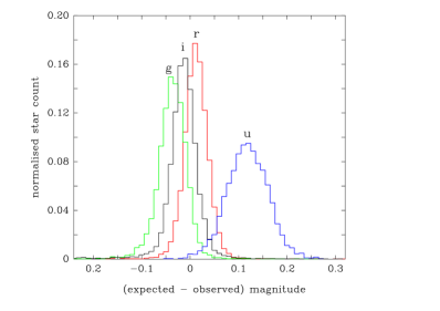
Figure 18: The distributions, by band pass, of the measured magnitude differences between VST test data and SDSS, after correction of the latter magnitudes from the AB to the Vega zero-magnitude scale. These were obtained from two VST pointings, away from the Galactic Plane, that overlap the SDSS footprint. The biggest differences are found in the $u$ band where the VST data are fainter than the corrected SDSS values by $\sim 0.12$, in the median.

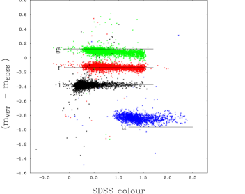
Figure 19: Measured magnitude shifts between VST and SDSS cross-matched objects as a function of SDSS colour, for the second of the two fields observed (only). The data in blue are $\Delta u$ versus $(u-g)_{SDSS}$; the data in green and red are, respectively, $\Delta g$ and $\Delta r$ versus $(g-r)_{SDSS}$; the data in black are $\Delta i$ versus $(r-i)_{SDSS}$. The horizontal lines show where the four loci would be expected to lie in the case that the SDSS and VST broadband filters were identical, and the calibrations perfect. The data fall into loci that are not far displaced from these horizontal lines and are almost as flat: this indicates that the colour-dependent terms that would be needed in equations to transform between the SDSS and VST systems are small.

In fig 18 we plot the histograms of the magnitude differences between the two surveys, according to pass band – pooling the data from both pointings. If the starting assumption is that the VST broadband filters are identical to the SDSS set, the predicted magnitude for each star in each filter is the measured SDSS magnitude, less the offset between the AB and Vega scales (essentially the numerical difference between the magnitude of Vega in the AB system and its value of 0.02 to 0.03, according to the alternative Vega-based convention – see table 8 in Fukugita et al 1996). In the $g$, $r$ and $i$ bands, the predicted and observed magnitudes are well-enough aligned, and the interquartile spread is consistent with the way the data were selected for random errors less than 0.03. However in $u$ there is a discrepancy that exceeds expected error: the median difference deviates by 0.12 magnitudes and the width of the distribution is twice that arising in the comparisons of the other bands.

The fuller picture is presented in figure 19 which shows the broadband magnitude differences as a function of the relevant SDSS colour for the second of our two fields (only). In all 4 pass bands, including $u$, the colour dependence can be seen to be very weak in that the loci traced out by the plotted stars are – to a first approximation – flat. The discrepancy seen in $u$ is revealed as mainly a zero-point shift, combined with scatter that exceeds the formal errors. In highly reddened Galactic Plane fields, the stellar colour effects may become more pronounced as extinction modifies the effective sampling of the passbands.

Table 5: Mean magnitude offsets between VST photometry and cross-matching synthetic photometry derived from the SDSS database of spectra. The synthetic magnitude scale adopts magnitudes for Vega itself of 0.026 (see Bohlin & Gilliland 2004)

Offset	Field 1 (117 stars)	Field 2 (50 stars)
$u_{VST}-u_{syn}$	0.07$\pm$0.39	0.11$\pm$0.17
$g_{VST}-g_{syn}$	0.06$\pm$0.09	0.06$\pm$0.04
$r_{VST}-r_{syn}$	0.01$\pm$0.06	0.03$\pm$0.03
$i_{VST}-i_{syn}$	-0.06$\pm$0.08	-0.05$\pm$0.03

As a separate exercise, we have used SDSS spectra to synthesise magnitudes and colours for stars with cross-matching VST photometry. The spectral type range present within this much smaller sample runs from B-type through to early M-type (M1). At wavelengths below 3800 Å falling within the $u$ band, it was necessary to extrapolate the spectra using appropriately chosen P98 library data. The result of this comparison is agreement between the VST and synthesised magnitudes at the $\sim$5 percent level (table 5), with the $u$ band as the outlier exhibiting much more pronounced scatter as well as somewhat higher offset. This pattern echoes the behaviour apparent in the VST-SDSS purely photometric comparison of fig 18, using a much larger sample. The difficulty is not confined to VST $u$ however, in that SDSS $u$ photometry fares scarcely any better relative to synthesis from the spectra (for the two fields, offset and scatter are -0.09 $\pm$ 0.37, and -0.04 $\pm$ 0.16). As more blue survey data are accumulated, it may become clear that the $u$ zeropoint will benefit from being tied to that of $g$ for those fields observed in the best conditions, as is presently done for $H\alpha$ with respect to $r$. This option is not yet enacted. For the time being, it must be acknowledged that pipeline $u$ calibration is more approximate than those of the other bands.

We have also used the reduced cross-match sample to look at how the VST photometric $r-H\alpha$ colour compares with its counterpart synthesised from spectra – looking, in particular, for any trends as a function of distance from field centre. No such trend is apparent, thereby meeting the expectation that the narrowband fluxes of normal stars, to early-M spectral type, would not be affected by the pattern of bandpass shifts discussed earlier in section 3 (cf. fig 10). However we do find that in order to make this detailed comparison, systematic offsets had to be removed from the VST photometry first. These were 0.075 in $(r-i)$, in the sense that the VST colours were too red by this amount, and a 0.02 reduction in $(r-H\alpha)$. The $(r-i)$ offset is consistent with the broadband magnitude offsets listed in Table 5 and hence is as expected. The $(r-H\alpha)$ adjustment is small enough (i.e. within the fit error) that it supports the zeropoint shift of 3.01 magnitudes between the $r$ and $H\alpha$ bands that was identified in section 4). Once these colour offsets are applied to the VST data, the rms scatter of the photometric $(r-H\alpha)$ colour relative to its synthetic counterpart is 0.04 for objects brighter than $r=19$.

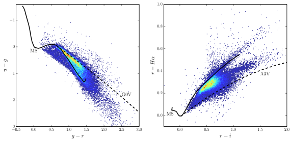
Figure 20: Left, the $(u-g,g-r)$ and right, the $(r-H\alpha,r-i)$ photometric diagrams pertaining to VPHAS+ survey field 1679. Both diagrams are plotted as two-dimensional stellar-density histograms, rainbow colour-coded such that high source densities (80-90 per bin) are red and the lowest densities (one per bin) are dark blue. The binning is 0.017$\times$0.025 in the left panel, 0.013$\times$0.008 in the right. The synthetic unreddened main sequence is drawn in, in black, in both panels. The G0V and A3V reddening lines obtained for $R=3.1$, drawn as black dashed lines, are included in respectively the $(u-g,g-r)$ and $(r-H\alpha,r-i)$ diagrams as useful aids to interpretation.

6 An example of point-source photometry derived from a VPHAS+ field

The extracted point-source photometry from the VST square-degree field is one of the two main data products from VPHAS+ – the other being the images themselves, considered below in section 7. We present an example of the two essential colour-colour diagrams in fig 20, in which band-merged stellar photometry for field 1679 is compared with the primary diagnostic synthetic tracks presented in section 4. This field includes the sky area from which data were taken to construct fig 6 illustrating typical errors. The massive open cluster, Westerlund 2, is located in the NE of these pointings, and the field as a whole includes moderate levels of diffuse, complex Hii emission. The data presented are drawn from a sky area centred on RA 10 24 49 Dec -57 58 00 (J2000) that spans 1.3 sq.deg – the total footprint occupied by the two offset positions.

Only objects with stellar point-spread functions in $g$, $r$ and $i$, brighter than $g=20$ are included in fig 20. Where two sets of magnitudes are available, the mean values have been computed and used. A further requirement imposed is that the random error in all bands may not exceed 0.1. The same $\sim$37000 objects are included in both diagrams. In order to obtain the diagrams shown, the pipeline photometric calibration was checked and refined as follows: we

• cross-matched brighter stars to APASS $g$, $r$ and $i$ photometry

• computed the median magnitude offset (applying no colour corrections – it was shown in fig 19 these are modest)

• corrected all $g$, $r$ and $i$ for these offsets;

• corrected $u$ by determining the vertical shift needed in the $(u-g,g-r)$ diagram to align the main stellar locus with the unreddened main sequence and the G0V reddening line

• corrected the $H\alpha$ zeropoint and hence all $H\alpha$ magnitudes according to the requirement that $zpt(H\alpha)=zpt(r)-3.01$.

This resulted in the following broadband corrections:- $\Delta i=-0.004$, $\Delta r=-0.032$ (red filter set), $\Delta r=-0.033$ (blue filter set), $\Delta g=0.069$ and $\Delta u=-0.31$. As expected, the correction that had to be applied to the $u$ photometry was, by far, the largest.

The main stellar locus can be seen to be tightly concentrated in both the blue and the red diagrams, and to favour lightly reddened G and K stars. The superimposed synthetic reddening lines (G0V in the $(u-g,g-r)$ diagram, A3V in $(r-H\alpha,r-i)$) have been drawn adopting the $R=3.1$ reddening law widely regarded as the Galactic norm. The blue diagram provides examples of three distinct typical populations falling outside the main stellar locus. Below it, at $(u-g)>1.5$ and $(g-r)>1.5$ (roughly) the plotted objects will mainly be M giants. Above the main stellar locus toward the red end, in the ranges $0<(u-g)<0.5$ and $1.5<(g-r)<2.0$ lie the OB stars in and around Westerlund 2. Finally, the modest scatter of blue objects lying above the G0V line roughly in the $0\leq(g-r)\leq 1$ range will include intrinsically-blue lightly-reddened subluminous objects.

It is interesting to note in the red diagram that there is some evidence that early-A stars making up the lower edge of the main stellar locus would better follow a different law, with $R\sim 3.8$ (see the tables in the Appendix). Indeed a reddening law of this type has been inferred for the OB stars in Westerlund 2 by Vargas Alvarez et al (2013). Most of the thin scatter of points below the main stellar locus, and some of the scatter above, in this same diagram will be the product of inaccurate background subtraction in H$\alpha$. But many of the objects lying above the main stellar locus will indeed be emission line objects, and some of the stars below will be white dwarfs. As expected, the red spurs of M dwarfs and M giants are broader features than their IPHAS counterparts (cf fig 17 and associated remarks).

For more discussion of these colour-colour diagrams, the reader is referred to Groot et al (2009, UVEX) and Drew et al (2005, IPHAS).

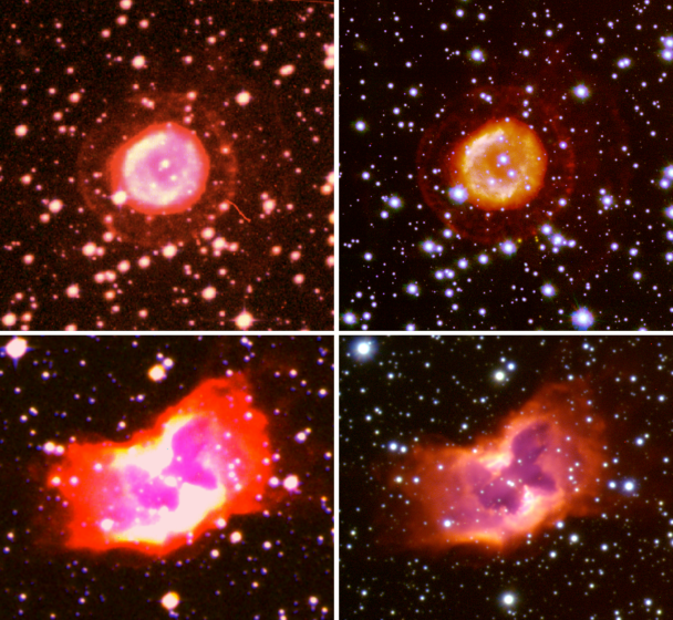
Figure 21: Two planetary nebulae, NGC 2438 (top) and NGC 2899 (bottom), as they appear in the SHS and VPHAS+ surveys. The SHS images are shown in the left-hand panels, with the VPHAS+ images to the right. The bands used to form them are: NGC 2438 – SHS R/G/B = $H\alpha$/SR/SSS Bj, VPHAS+ R/G/B = $H\alpha$/$r$/$i$, NGC 2899 – SHS R/G/B = $H\alpha$/SR/SSS Bj, VPHAS+ R/G/B = $H\alpha$/$r$/$g$. The cut-out image dimensions are 300$\times$300 arcsec² for NGC 2438, and 200$\times$180 arcsec² for NGC 2899.

7 Nebular astrophysics with VPHAS+ images

Just over a decade ago the SuperCOSMOS H$\alpha$ Survey (SHS, Parker et al 2005) had only just completed. This was the last survey using photographic emulsions that the UK Schmidt Telescope undertook. The 3-hour narrowband H$\alpha$ filter exposures reach a very similar limiting surface brightness to the 2 minute exposures VPHAS+ is built around. Hence, the differences in capability are not about sensitivity, as this is roughly the same in the two surveys. Instead it is about the great improvement in dynamic range on switching to digital detectors, the good seeing of the VST’s Paranal site, and the added broad bands.

SHS, with its enormous 5-degree diameter field, has been comprehensively trawled for southern planetary nebulae (the MASH catalogue, Parker et al 2006, Miszalski et al 2008). The remaining discovery space for resolved nebulae is expected to be at low surface brightnesses in locations of high stellar density, and in the compact domain around and below the limits of the typical spatial resolution of SHS ($\sim 0.5$ to 3.0 arcsec). Both these conditions will most often be met in the Galactic Bulge, at a mean distance of $\sim$8 kpc. Data-taking in the Bulge and its maximally-dense star fields is planned to begin in mid 2014.

Among planetary nebulae (PNe), small angular size is due either to great distance or to youth – the study of either compact category provides exciting possibilities. As well as the Bulge, the less-studied outer parts of the Galactic Plane should be searched. In this respect, IPHAS, with its direct view to the Galactic Anticentre is better positioned: the ongoing study of the Anticentre PN population has revealed dozens of new candidates (Viironen et al. 2009a), including the PN with the largest galactocentric distance to date (20.8 $\pm$ 3.8 kpc, Viironen et al 2011). By following up such finds to measure chemical abundances, crucial beacons are obtained for the study of the Galactic abundance gradient and its much disputed flattening towards the largest galactocentric radii. VPHAS+ completed the access to the outer Plane over the longitude range $215^{\circ}<\ell<270^{\circ}$.

Data from both IPHAS and VPHAS+ can make fundamental contributions to the study of very young PNe – particularly by helping to solve the two-decades-old puzzle of how PNe already emerge with the observed wide variety of morphologies (round, elliptical, bipolar, multipolar, point-symmetric, etc. – see Sahai et al. 2011). What does this variety say about the properties of their AGB progenitors? Detailed studies of objects in the phases preceding the PN phase – AGB and post-AGB stars, proto-PNe, and transition or PN-nascent objects – are underway (e.g. Sanchez Contreras & Sahai 2012). Superb imaging capabilities like those of the VST, accessed via VPHAS+, will support this work.

Indeed there is a serious paucity of very small PNe in the existing optical catalogues: there are no PNe with angular extent less than 3 arcsec in the MASH catalogue (out of 903 objects; Parker et al 2006), and only 8 PNe in the catalogue by Tylenda et al (2003, 312 objects) in the size range 1.4 – 3 arcsec. There is just one with a confidently-measured diameter below 1 arcsec in the larger Strasbourg Catalogue of PNe (1143 objects; Acker et al. 1994), that happens to be a Bulge PN. IPHAS has demonstrated that extremely young compact PNe can be reached (Viironen et al, 2009b), while Sabin et al (in prep.) have found some 20 new PNe with diameters of 1-3 arcsec in by-eye searchs of IPHAS image mosaics. Even smaller, but brighter, nebulae around symbiotic stars of the dusty D subtype are emerging – the record so far being IPHASJ193943.36+262933.1, a new D symbiotic star with an $H\alpha$ extent of only 0.12 arcsec that has been confirmed via HST imaging and recently studied with the 10.4m GTC telescope (Rodriguez Flores et al. 2014, submitted to A&A).

Apart from opening up new discoveries, a further benefit of good seeing is the clearer view of nebular structure that it offers. This is nicely demonstrated in fig 21. SHS and VPHAS+ detect the main features of the planetary nebulae NGC 2438 and NGC 2899 to very similar depth – for example, the fainter outer halo is just detected in both versions of NGC 2438. But, evidently, the VPHAS+ images better resolve the fine sculpting within both nebulae as a consequence of the seeing FWHM being under a half that prevailing in SHS data. The extended dynamic range of VPHAS+ helps in this respect, too, in that early saturation also obliterates detail. This advantage is especially clear in the images of NGC 2899, where the structure in the bright nebulous lobes is preserved in VPHAS+, but is entirely bleached out in SHS. The more the level of detail that can be picked out, the more certain and subtle morphological classifications and interpretations can become.

The combination of good seeing and high dynamic range also makes the separation of fainter stars from background nebulosity much easier. This capability is critically important to the study of the young massive clusters, still swathed in diffuse Hii emission, where the analysis of stellar content is very much a focus of continuing research. For example, Feigelson et al (2013) have offered a critique of the nuisance created by spatially-complex nebulosity. The obvious answer to this and the problem of dust obscuration is to turn to selection using NIR and X-ray data. Nevertheless the availability of imaging data of the high quality seen in VPHAS+ data will make it possible to extend SEDs for many more stars into the effective-temperature (and reddening) sensitive optical domain. In addition, understanding the shaping of the interstellar medium in star-forming environments remains an important part of the picture (see e.g. Wright et al 2012 on proplyd-like structures in Cyg OB2). The detail that the VST is capable of revealing both in obscuration and ionised hydrogen in star-forming regions can be quite exquisite. Here, in fig 22, we illustrate this with an excerpt from VPHAS+ data on the Lagoon Nebula, showing the fine tracing of the shapes of dark globules and eroding dusty structures that is achieved.

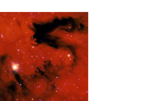
Figure 22: A cut-out at full resolution from M8, the Lagoon Nebula. This is an RGB image centred on RA 18 09 36 Dec -24 01 51 (J2000), and spanning 150$\times$150 arcsec². The filters are combined such that R/G/B = $H\alpha$/$i$/$r$.

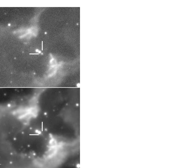
Figure 23: The central star of NGC 2899 reveals itself. The top panel is a 1$\times$1 arcmin² thumbnail of the centre of NGC 2899 as imaged through the $u$ filter, while the bottom is the corresponding $r$ thumbnail. The white right-angled bars pick out the position of an extremely blue, relatively faint star that is clearly present in all $u$ (and $g$) exposures obtained, but is too faint for detection in $r$.

In planetary and other evolved-star nebulae it is of course important to identify the ionising object. The search for missing PN central stars is a quest that VPHAS+ can aid greatly through the provision of spatially well-resolved $u$ and $g$ data. Indeed inspection of the data used to contruct fig 21 has revealed the probable central star of NGC 2899 for the first time. As shown in fig 23, there is very evidently a third very-blue star just SW of the pair of stars that have, in the past, been scrutinised as possible companions to what is required to be an extremely hot ($T_{eff}>250,000$ K), but probably faint central star (López et al 1991). This blue object was detected on the night of 20th December 2012 at a provisional $u$ magnitude of 18.79 $\pm 0.02$. It fades through $g$ (19.36 $\pm 0.02$) to become undetected by the pipeline, and scarcely visible to eye inspection, in $r$. Its coordinates are RA 09 27 02.72 Dec -56 -06 22.9 (J2000), just 1.7 arcsec from the more southerly of the pair of brighter stars examined before by López et al (1991). Based on the $g$ magnitude and an inferred $V$ flux, we have determined the central star’s effective temperature, via the well-established Zanstra method. Using the reddening and integrated H$\alpha$ flux from López et al and Frew, Bojičić & Parker (2013) respectively, we estimate $T_{\rm z,H}=215\pm 16$ kK. This is cooler than the temperature given by López et al, based on the ’crossover’ method, but still extraordinarily hot for a central star well down the white-dwarf cooling track.

It was one of the major science drivers for the merged VPHAS+ survey that $u$ data, supported by $g$, would result in the detection of a broad range of intrinsically very blue objects – be they PN central stars, interacting binaries or massive OB and Wolf-Rayet stars. An extreme example like NGC 2899’s central star provides the useful lesson that selection via the $u-g,g-r$ colour-colour diagram would have failed to pick it out – because of the non-detection in $r$. In a case like this, the $u,u-g$ colour-magnitude diagram has to be examined, in tandem with the appropriate images.

8 VPHAS+ photometry as a reference set for variability studies

As the northern survey, IPHAS, has progressed over the decade since 2003, there have been occasions on which it was possible to use the growing database as a high-quality reference for checking transient reports – particularly of novae. The most spectacular IPHAS example of this was the nova and variable, V458 Vul (Wesson et al 2008; Rodriguez-Gil et al 2010) where the eruption occurred a few months after obtaining H$\alpha$ images revealing a pre-existing ionised nebula around the star. Indeed there have been several instances in which photometry of the progenitor object has been extracted from the IPHAS database and has been used to gain insight into the prior presence or absence of line emission or to set constraints on likely extinction (Steeghs et al 2007, Greimel et al 2012). Such opportunities will certainly arise with VPHAS+ – and be richer given the five filters offered.

In the southern hemisphere novae will be more frequent, as will other transient events. Furthermore responses to alerts, or the need to demonstrate long-term flux variations, can bring into use repeats of observations made necessary by initial quality-control failures. An example of this is provided by Vink et al (2008) who used repeat IPHAS observations – taken on account of poor observing conditions – to discuss the LBV candidacy of G79.29$+$0.46. With the increased attention being given to the reporting and exploitation of transient objects (including the forthcoming Gaia alerts programme), this use of VPHAS+ will become more common.

9 Summary and concluding remarks

This paper has introduced and defined VPHAS$+$, the VST Photometric $H\alpha$ Survey of the Southern Galactic Plane and Bulge. The data taking, the rationale behind it, the data processing and data quality have all been described. The properties and limitations of the survey’s narrowband H$\alpha$ filter, NB-659, have been laid out and simulated in order to anticipate its performance. In addition we have provided tables of the expected photometric colours of normal solar-metallicity stars to aid the interpretation of the survey’s characteristic photometric diagrams – most are to be found in the Appendix where the effect of changing the adopted reddening law is illustrated. The VPHAS+ H$\alpha$ filter transmission is redder, wider and $\sim 20$ % higher-throughput than its IPHAS counterpart – a difference that feeds through to noticeably different $(r-H\alpha)$ colours for M stars.

We have validated the photometry that is delivered by VST/OmegaCAM and subsequently pipelined at CASU, using test data taken of a field for which SDSS photometry is available. We find the agreement is satisfactory, with the $g$, $r$ and $i$ band calibrations differing by between 0.01 to 0.05 magnitudes. However, for the time being, the pipeline calibration should be regarded as provisional – it will undoubtedly improve. Examples of the excellent imaging performance of the VST/OmegaCAM combination relative to previous surveys have been provided, and we draw attention to the valuable archival role this first digital survey can fulfill in supporting discoveries of transient sources.

Exploitation of the survey is now beginning. The detection of a compact ionized nebula around W26, the extreme M supergiant in Westerlund 1 has already been published (Wright et al 2014). Applications have been made for follow-up spectroscopy that will test the quality of selection of specialised object types that VPHAS+ photometry makes possible. Progress is also being made via direct analyses of the photometry. For example, Mohr-Smith et al (in prep.) are conducting a search for OB stars in the vicinity of the massive cluster Westerlund 2, and they are finding a close match between the properties of known cluster O stars as derived from VPHAS+ data and those inferred by Vargas Alvarez et al (2013, see also Drew et al 2013). This and other early appraisals of the data indicate that VPHAS+ will be an excellent vehicle for automated searches for reddened early-type stars. Kalari et al (in prep.) are employing both narrow-band H$\alpha$ and the broadbands to measure mass-accretion rates in pre-main-sequence stars: they are finding that H$\alpha$ mass-accretion rates in T Tauri stars compare favourably to rates determined from the $u$ band in the case of the Lagoon Nebula, NGC 6530.

As the calibration of the survey data improves, the measurement of accurate integrated H$\alpha$ fluxes for many faint southern PNe and other extended objects becomes possible, and will extend the work of Frew et al (2013, 2014). In due course these fluxes can be compared with existing and also new radio continuum fluxes coming on stream (see e.g. Norris et al 2011) in order to determine reliable extinction values for many faint nebulae currently lacking data. This technique has already been applied to the case of W26 in Westerlund 1 (Wright et al 2014).

When it becomes possible to cross-match VVV and VPHAS$+$ data, it will open up the power of homogeneous photometric mapping of the central parts of the Galactic Plane in up to 10 photometric bands spanning both the optical and the near-infrared. Beyond the VVV sky area, there is a synergy to be exploited in bringing VPHAS+ data together with those of the all-sky 2MASS survey (Skrutskie et al 2006) and with the UKIDSS Galactic Plane Survey (Lucas et al 2008), in those parts of the first and third Galactic quadrants the latter has covered. It is worth noting, however, that 2MASS alone is too shallow to link effectively with VPHAS+ for sightlines where the integrated visual extinction is less than $\sim 5$ magnitudes. This does mean that the longitude range $230^{\circ}<\ell<300^{\circ}$, in particular, is presently lacking sufficiently deep NIR photometry. In the longer term, many of the sources of interest that VPHAS+ finds will benefit from accurate parallaxes and other data from ESA’s Gaia mission – given the similar sensitivity limits reached. Conversely in the meantime, VPHAS+ has already begun to assist ambitious wide-field spectroscopy programmes such as the Gaia-ESO Survey (Gilmore et al 2012) through the provision of the wide-field photometry needed for target selection and field setup.

By the end of 2013, 25% of all observations making up the survey had been obtained to the required quality, and in May 2013 a first release of single-band catalogues was made to the ESO archive that contained roughly 10% of the eventual total (based on data obtained prior to 15 October 2012). By design, the characteristics of VPHAS+ are similar to those of the IPHAS and UVEX Galactic plane survey pair in the north. In particular, the double-pass strategy is shared, with the result that the majority of detected objects are picked up and measured twice, with no more than $\sim$0.1 percent of objects missed altogether. This feature has informed the way in which the IPHAS DR2 catalogue (Barentsen et al, 2014) has been constructed – and it is intended that a first band-merged VPHAS+ catalogue, for public release, will be built along analogous lines during the second half of 2014. This will incorporate data from the first 3 seasons of VST observing, and give a complete photometric account of the Galactic mid-plane. For ease of use, for every detected source, the catalogue will provide a single recommended set of magnitudes in up to 5 optical bands.

Appendix A Synthetic colour reddening tables

Synthetic colours for main sequence stars, computed as described in Section 4, are tabulated in full in an online supplement for three representative reddening laws ($R_{V}=2.5$, 3.1 and 3.8) and a range of reddenings ($A_{0}=0$, 2, 4, 6, 8, 10). The form of the reddening laws used is due to Fitzpatrick & Massa (2007). As an example of the tables available we include excerpts from the second and fifth tables that respectively provide $R_{V}=3.1$ blue-filter and red-filter colours for B,A main-sequence stars.

Two further tables of synthetic colours are included in the supplement for K-M giants that have been computed using P98 library spectra. Data are provided for the $R=3.1$ mean Galactic law only, for the limited purposes of (a) giving an impression of how these luminous red objects may contaminate $(u-g,g-r)$ diagrams at redder $(g-r)$ through $u$ red leak (b) enabling comparisons with the M-giant spur commonly seen in $(r-H\alpha,r-i)$ colour-colour diagrams.

Table 6: VST/OmegaCAM synthetic colours for B,A main-sequence stars in the $(u-g),(g-r)$ plane reddened with an $R_{V}=3.1$ extinction law. (Full table online.)

Spectral	$A_{0}=0$		$A_{0}=2$		$A_{0}=4$		$A_{0}=6$		$A_{0}=8$
Type	$(u-g)$	$(g-r)$	$(u-g)$	$(g-r)$	$(u-g)$	$(g-r)$	$(u-g)$	$(g-r)$	$(u-g)$	$(g-r)$
$B0V$	$-1.433$	$-0.271$	$-0.692$	$0.529$	$0.087$	$1.301$	$0.891$	$2.050$	$1.632$	$2.777$
$B1V$	$-1.324$	$-0.240$	$-0.584$	$0.558$	$0.195$	$1.329$	$0.995$	$2.076$	$1.719$	$2.802$
$B2V$	$-1.209$	$-0.218$	$-0.470$	$0.579$	$0.307$	$1.350$	$1.104$	$2.096$	$1.808$	$2.821$
$B3V$	$-1.053$	$-0.186$	$-0.315$	$0.610$	$0.460$	$1.379$	$1.250$	$2.125$	$1.923$	$2.849$
$B5V$	$-0.828$	$-0.139$	$-0.092$	$0.655$	$0.680$	$1.423$	$1.460$	$2.166$	$2.080$	$2.890$
$B6V$	$-0.728$	$-0.121$	$0.007$	$0.672$	$0.776$	$1.439$	$1.550$	$2.182$	$2.144$	$2.905$
$B7V$	$-0.580$	$-0.100$	$0.152$	$0.692$	$0.918$	$1.458$	$1.682$	$2.200$	$2.234$	$2.922$
$B8V$	$-0.388$	$-0.076$	$0.340$	$0.714$	$1.101$	$1.478$	$1.850$	$2.219$	$2.344$	$2.940$
$B9V$	$-0.198$	$-0.046$	$0.528$	$0.742$	$1.285$	$1.504$	$2.019$	$2.244$	$2.445$	$2.964$
$A0V$	$-0.053$	$-0.005$	$0.675$	$0.780$	$1.431$	$1.540$	$2.153$	$2.277$	$2.514$	$2.995$
$A1V$	$-0.019$	$0.005$	$0.709$	$0.790$	$1.464$	$1.550$	$2.181$	$2.287$	$2.525$	$3.005$
$A2V$	$0.021$	$0.025$	$0.749$	$0.809$	$1.505$	$1.568$	$2.217$	$2.304$	$2.538$	$3.021$
$A3V$	$0.038$	$0.059$	$0.771$	$0.840$	$1.531$	$1.597$	$2.241$	$2.332$	$2.541$	$3.048$
$A5V$	$0.067$	$0.125$	$0.805$	$0.904$	$1.567$	$1.658$	$2.269$	$2.390$	$2.523$	$3.105$
$A7V$	$0.044$	$0.199$	$0.788$	$0.975$	$1.554$	$1.726$	$2.252$	$2.456$	$2.474$	$3.169$

Table 7: VST/OmegaCAM synthetic colours for B,A main-sequence stars in the $(r-i),(r-H\alpha)$ plane reddened with an $R_{V}=3.1$ extinction law. (Full table online.)

Spectral	$A_{0}=0$		$A_{0}=2$		$A_{0}=4$		$A_{0}=6$		$A_{0}=8$		$A_{0}=10$
Type	$(r-i)$	$(r-H\alpha)$	$(r-i)$	$(r-H\alpha)$	$(r-i)$	$(r-H\alpha)$	$(r-i)$	$(r-H\alpha)$	$(r-i)$	$(r-H\alpha)$	$(r-i)$	$(r-H\alpha)$
$B0V$	$-0.150$	$0.054$	$0.278$	$0.198$	$0.694$	$0.316$	$1.100$	$0.409$	$1.496$	$0.478$	$1.884$	$0.526$
$B1V$	$-0.136$	$0.048$	$0.291$	$0.192$	$0.708$	$0.310$	$1.114$	$0.403$	$1.510$	$0.472$	$1.898$	$0.519$
$B2V$	$-0.123$	$0.045$	$0.304$	$0.188$	$0.721$	$0.306$	$1.126$	$0.398$	$1.523$	$0.466$	$1.911$	$0.513$
$B3V$	$-0.104$	$0.044$	$0.323$	$0.186$	$0.740$	$0.303$	$1.145$	$0.394$	$1.541$	$0.462$	$1.929$	$0.508$
$B5V$	$-0.077$	$0.039$	$0.349$	$0.180$	$0.765$	$0.295$	$1.170$	$0.386$	$1.566$	$0.452$	$1.954$	$0.497$
$B6V$	$-0.068$	$0.036$	$0.358$	$0.177$	$0.774$	$0.291$	$1.179$	$0.381$	$1.575$	$0.448$	$1.963$	$0.492$
$B7V$	$-0.057$	$0.029$	$0.369$	$0.170$	$0.785$	$0.284$	$1.190$	$0.374$	$1.586$	$0.440$	$1.973$	$0.484$
$B8V$	$-0.045$	$0.018$	$0.382$	$0.158$	$0.797$	$0.272$	$1.202$	$0.362$	$1.598$	$0.427$	$1.985$	$0.471$
$B9V$	$-0.028$	$0.006$	$0.398$	$0.145$	$0.813$	$0.259$	$1.218$	$0.348$	$1.614$	$0.413$	$2.001$	$0.456$
$A0V$	$-0.009$	$-0.005$	$0.418$	$0.133$	$0.833$	$0.246$	$1.238$	$0.334$	$1.633$	$0.399$	$2.020$	$0.441$
$A1V$	$-0.003$	$-0.003$	$0.423$	$0.135$	$0.838$	$0.248$	$1.243$	$0.335$	$1.638$	$0.399$	$2.025$	$0.442$
$A2V$	$0.006$	$-0.004$	$0.432$	$0.134$	$0.847$	$0.247$	$1.251$	$0.334$	$1.646$	$0.397$	$2.033$	$0.439$
$A3V$	$0.021$	$-0.008$	$0.446$	$0.130$	$0.861$	$0.241$	$1.265$	$0.328$	$1.660$	$0.391$	$2.047$	$0.432$
$A5V$	$0.051$	$0.005$	$0.476$	$0.141$	$0.890$	$0.250$	$1.293$	$0.335$	$1.687$	$0.396$	$2.073$	$0.436$
$A7V$	$0.083$	$0.027$	$0.507$	$0.160$	$0.920$	$0.268$	$1.322$	$0.350$	$1.716$	$0.410$	$2.101$	$0.448$

References

- [Abazajian et al2009] Abazajian K. N., et al., 2009, ApJS, 182, 543
- [Acker et al1994] Acker A., Ochsenbein F., Stenholm B., et al. 1994, VizieR Online Data Catalog, 5084, 0
- [Barentsen et al2011] Barentsen G., et al., 2011, MNRAS, 415, 103
- [Barentsen et al2014] Barentsen G., et al., 2014, in preparation
- [Beaulieu et al2000] Beaulieu S. F., Freeman K. C., Kalnajs A. J., Saha P., Zhao H. 2000, AJ, 120, 855
- [Bohlin & Gilliland2004] Bohlin R. C., Gilliland R. L., 2004, AJ, 127, 3508
- [Corradi et al2010] Corradi R. L. M., et al., 2010, A&A, 509, 41
- [Dopita & Hua1997] Dopita M. A., Hua C. T., 1997, ApJS, 108, 515
- [Drew et al2005] Drew J. E., et al., 2005, MNRAS, 362, 753
- [Drew et al2013] Drew J. E., et al., 2013, The Messenger, 154, 41
- [Drimmel & Spergel2001] Drimmel R., Spergel D., 2001, 556, 181
- [Durand et al1998] Durand S., Acker A., Zijlstra A., 1998, A&AS, 132, 13
- [Feigelson et al2013] Feigelson, E. D., et al., 2013, ApJS, 209, 26
- [Finkbeiner et al2004] Finkbeiner D. P., et al., 2004, AJ, 128, 2577
- [\citennameFitzpatrick & Massa2007] Fitzpatrick E. L., Massa D., 2007, ApJ, 663, 320
- [Fitzpatrick & Massa2009] Fitzpatrick E. L., Massa D., 2009, ApJ, 699, 1209
- [Frew et al2013] Frew D. J., Bojičić, I. S., Parker Q. A., 2013, MNRAS, 431, 2
- [Frew et al2014] Frew D. J., Bojičić, I. S., Parker Q. A., Pierce M. J., Gunawardhana M. L. P., Reid W. A., 2014, MNRAS, in press (arxiv:1303.4555)
- [Fukugita et al1996] Fukugita M., Ichikawa T., Gunn J. E., Doi M., Shimasaku K., Schneider D. P., 1996, AJ, 439, 584
- [Gilmore et al2012] Gilmore G., et al., 2012, The Messenger, 147, 25
- [Gonzalez-Solares et al2008] Gonzalez-Solares E., et al., 2008, MNRAS, 388, 89
- [Greimel et al2012] Greimel R., Drew J. E., Steeghs D., Barlow M. J., 2012, ATel, no.4365
- [Groot et al2009] Groot P. J., et al., 2009, MNRAS, 399, 323
- [Hayes1985] Hayes D. S., 1985, in Calibration of fundamental stellar quantities, Proc. IAU Sym. No.111, Dordrecht, D. Reidel Publishing Co., pp225-249
- [Irwin 19851985] Irwin M. J., 1985, MNRAS, 214, 575
- [Irwin et al2004] Irwin M. J., et al., 2004, SPIE, 5493, 41
- [Irwin & Lewis2001] Irwin M. J., Lewis J., 2001, NewAR, 45, 1051
- [Irwin2010] Irwin M. J., 2010, UKIRT Spring Newsletter, p14
- [Kuijken2011] Kuijken K., 2011, The Messenger, 146, 8
- [Lopez et al1991] López J. A., Falcon L. H., Ruiz M. T., Roth M., 1991, A&A, 241, 526
- [Landolt1992] Landolt A. U., 1992, AJ, 104, 340
- [Lucas et al2008] Lucas P. W., 2008, MNRAS, 391, 136
- [Marshall etal2006] Marshall D. J., Robin A. C., Reylé C., Schultheis, M., Picaud, S., 2006, A&A, 453, 635
- [Minniti et al2011] Minniti D., et al., 2010, NewA, 15, 433
- [Miszalski et al2008] Miszalski B., Parker Q. A., Acker A., Birkby J. L., Frew D. J., Kovacevic A., 2008, MNRAS, 384, 525
- [Norris et al2011] Norris R. P., et al., 2011, PASA, 28, 215
- [Parker et al2005] Parker Q.A., et al, 2005, MNRAS, 362, 689
- [Parker et al2006] Parker Q. A., et al, 2006, MNRAS, 373, 79
- [Patat et al2011] Patat F., et al., 2011, A&A, 527, 91
- [Pickles1998] Pickles A. J., 1998, PASP, 110, 863 (P98)
- [Raddi et al2013] Raddi R., et al, 2013, MNRAS, 430, 2169
- [Rodriguez-Gil et al2010] Rodriguez-Gil P., et al, 2010, MNRAS, 407 L21
- [Sahai et al2011] Sahai R., Morris M. R., Villar G. G., 2011, AJ, 141, 134
- [Sale et al2009] Sale S. E., et al., 2009, MNRAS, 392, 497
- [Sale2012] Sale S. E., 2012, MNRAS, 427, 2119
- [Sanchez-Contreras & Sahai2012] Sanchez-Contreras C., Sahai R., 2012, ApJS, 203, 16
- [Schlegel et al1998] Schlegel D. J., Finkbeiner D. P., Davis M., 1998 ApJ, 500, 525
- [Skrutskie et al2006] Skrutskie, M. F., et al., 2006, AJ, 131,1163
- [Steeghs et al2007] Steeghs D., et al., 2007, Atel, no. 795
- [Stephenson & Sanduleak1971] Stephenson C. B., Sanduleak N., 1971 PW&SO 1, 1 (SS71)
- [Straizys & Kuriliene1981] Straizys V., Kuriliene G., 1981, Ap&SS, 80, 353
- [Taylor2005] Taylor M. B., 2005, ASPC, 347, 29
- [Tylenda et al2003] Tylenda R., Si dmiak N., Górny S. K., Corradi R. L. M., Schwarz H. E., 2003, A&A, 405, 627
- [Valdivieso et al2009] Valdivieso, L., et al., 2009, A&A, 497, 973
- [Verbeek et al2012a] Verbeek K., et al., 2012a, MNRAS, 420, 1115
- [Verbeek et al2012b] Verbeek K., et al., 2012b, MNRAS, 426, 1235
- [Viironen et al2009a] Viironen K., et al., 2009a, A&A, 504, 291
- [Viironen et al2009] Viironen K., et al., 2009b, A&A, 502, 113
- [Viironen et al2011] Viironen K., et al., 2011, A&A, 530, 107
- [Vink et al2008] Vink J. S., Drew J. E., Steeghs D., Wright N. J., Martin E. L., Gänsicke B. T., Greimel R., Drake J., 2008, MNRAS, 387, 308
- [Wesson et al2008] Wesson R., et al., 2008, ApJ, 688, L21
- [Witham et al2006] Witham A. R., et al., 2006, MNRAS, 369, 581
- [Wright et al2008] Wright N. J., et al., 2008, MNRAS, 390, 929
- [Wright et al2012] Wright N. J., Drake J. J., Drew J. E., Guarcello M. G., Gutermuth R. A., Hora J. L., Kraemer K. E., 2012, ApJ, 746, L21
- [Wright et al2014] Wright N. J., et al., 2014, MNRAS, 437, L1