Abstract

Bayesian optimization is a powerful global optimization technique for expensive black-box functions. One of its shortcomings is that it requires auxiliary optimization of an acquisition function at each iteration. This auxiliary optimization can be costly and very hard to carry out in practice. Moreover, it creates serious theoretical concerns, as most of the convergence results assume that the exact optimum of the acquisition function can be found. In this paper, we introduce a new technique for efficient global optimization that combines Gaussian process confidence bounds and treed simultaneous optimistic optimization to eliminate the need for auxiliary optimization of acquisition functions. The experiments with global optimization benchmarks and a novel application to automatic information extraction demonstrate that the resulting technique is more efficient than the two approaches from which it draws inspiration. Unlike most theoretical analyses of Bayesian optimization with Gaussian processes, our finite-time convergence rate proofs do not require exact optimization of an acquisition function. That is, our approach eliminates the unsatisfactory assumption that a difficult, potentially NP-hard, problem has to be solved in order to obtain vanishing regret rates.

1 Introduction

We consider the problem of approximating the maximizer of a deterministic black-box function $f:{\cal X}\mapsto\mathbb{R}$. The function $f$ can be evaluated point-wise, but it is assumed to be expensive to evaluate. More precisely, we assume that we are given a finite budget of $n$ possible function evaluations.

This global optimization problem can be treated within the framework of sequential design. In this context, by allowing $\mathbf{x}_{t}\in{\cal X}$ to depend on previous points and corresponding function evaluations ${\cal D}_{t-1}=\{(\mathbf{x}_{1},f(\mathbf{x}_{1})),\ldots,(\mathbf{x}_{t-1},f(\mathbf{x}_{t-1}))\}$, the algorithm constructs a sequence $\mathbf{x}_{1:n}=(\mathbf{x}_{1},\mathbf{x}_{2},\ldots,\mathbf{x}_{n})$ and returns the element $\mathbf{x}(n)$ of highest possible value. That is, it returns the value $\mathbf{x}(n)$ that minimizes the loss:

$$r_{n}=\sup_{\mathbf{x}\in{\cal X}}f(\mathbf{x})-f(\mathbf{x}(n)).$$

This loss is not the same as the cumulative regret used often in the online learning literature: $R_{n}=n\sup_{\mathbf{x}\in{\cal X}}f(\mathbf{x})-\sum_{t=1}^{n}f(\mathbf{x}(t)).$

Bayesian optimization (BO) is a popular sequential design strategy for global optimization; see Brochu et al. (2009) for an introductory treatment. Since the objective function $f$ is unknown, the Bayesian strategy is to treat it as a random function and place a prior over it. The prior captures our beliefs about the behaviour of the function. After gathering the function evaluations ${\cal D}_{t-1}$, the prior is updated to form the posterior distribution over $f$. The posterior distribution, in turn, is used to construct an acquisition function that determines what the next query point $\mathbf{x}_{t}$ should be. Examples of acquisition functions include probability of improvement, expected improvement, Bayesian expected losses, upper confidence bounds (UCB), and dynamic portfolios of these (Močkus, 1982; Jones, 2001; Garnett et al., 2010; Srinivas et al., 2010; Chen et al., 2012; Hoffman et al., 2011). If we were to implement Thompson sampling strategies (May et al., 2011; Kaufmann et al., 2012; Agrawal & Goyal, 2013) for Gaussian processes (GPs), we would also encounter the difficult problem of having to find the maximizer of a sample from the GP at each iteration, unless we were considering only a finite set of query points (Hoffman et al., 2014).

The maximum of the acquisition function is typically found by resorting to discretisation or by means of an auxiliary optimizer. For example, Snoek et al. (2012) use discretisation, Bardenet & Kégl (2010) use adaptive grids, Brochu et al. (2007); Martinez-Cantin et al. (2007) and Mahendran et al. (2012) use the DIRECT algorithm of Jones et al. (1993), Lizotte et al. (2011) use a combination of random discretisation and quasi-Newton hill-climbing, Bergstra et al. (2011) and Wang et al. (2013) use the CMA-ES method of Hansen & Ostermeier (2001), Hutter et al. (2011) apply multi-start local search. (Approaches within the framework of Bayesian nonlinear experimental design, such as (Hennig & Schuler, 2012) for finding maxima and (Kueck et al., 2006, 2009; Hoffman et al., 2009) for learning functions and Markov decision processes, have to rely on expensive approximate inference for computing intractable integrals. An analysis of these approaches is beyond the scope of this paper.)

The auxiliary optimization methodology is problematic for several reasons. First, it is difficult to assess whether the auxiliary optimizer has found the maximum of the acquisition function in practice. This creates important theoretical concerns about the behaviour of BO algorithms because the typical theoretical convergence guarantees are only valid on the assumption that the optimum of the acquisition function can be found exactly; see for example Srinivas et al. (2010); Vazquez & Bect (2010) and Bull (2011). Second, running an auxiliary optimizer at each iteration of the BO algorithm can be unnecessarily costly. For any two consecutive iterations, the acquisition function may not change drastically. This questions the necessity of re-starting the auxiliary optimization at each iteration.

Recent optimistic optimization methods provide a viable alternative to BO (Kocsis & Szepesvári, 2006; Bubeck et al., 2011; Munos, 2011). Instead of estimating a posterior distribution over the unknown objective function, these methods build space partitioning trees by expanding leaves with high function values or upper-bounds. The term optimistic, in this context, is used to refer to the fact that the algorithms expand at each round leaves that may contain the optimum. Remarkably, a variant of these methods, Simultaneous Optimistic Optimization (SOO) by Munos (2011), is able to optimize an objective function globally without knowledge of the function’s smoothness. SOO is optimistic at all scales in the sense that it expands several leaves simultaneously, with at most one leaf per level. For this reason, instead of adopting the term “Simultaneous OO” we opt for the descriptive term “Multi-Scale OO”.

We will describe SOO in more detail in Section 3. We also note that a stochastic variant of SOO has been recently proposed by Valko et al. (2013), but we restrict the focus of this paper to the deterministic case.

These optimistic optimization methods do not require the auxiliary optimization of acquisition functions. However, due to the lack of a posterior that interpolates between the sampled points, it is conceivable that these methods may not be as competitive as BO in practical domains where prior knowledge is available. This claim does not seem to have been backed up by empirical evidence in the past.

This paper introduces a new algorithm, BaMSOO, which combines elements of BO and SOO. Importantly, it eliminates the need for auxiliary optimization of the acquisition function in BO. We derive theoretical guarantees for the method that do not depend on the assumption that the acquisition function needs to be optimized exactly. The method uses SOO to optimize the objective function directly, but eliminates the need for SOO to sample points that are deemed unfit by Gaussian process posterior bounds. That is, BaMSOO uses the posterior distribution to reduce the number of function evaluations in SOO, thus increasing the efficiency of SOO substantially.

The experiments with benchmarks from the global optimization literature demonstrate that BaMSOO outperforms both GP-UCB and SOO. The paper also introduces a novel application in the domain of knowledge discovery and information extraction. Finally, our theoretical results show that BaMSOO can attain, up to log factors, a polynomial finite sample convergence rate.

2 BO with GP confidence bounds

Classical BO approaches have two ingredients that need to be specified: The prior and the acquisition function. In this work, as in most other works, we adopt Gaussian process (GP) priors. We review GPs very briefly and refer the interested reader to the book of Rasmussen & Williams (2006) for an in-depth treatment. A GP is a distribution over functions specified by its mean function $m(\cdot)$ and covariance $\kappa(\cdot,\cdot)$. More specifically, given a set of points $\mathbf{x}_{1:t}$, with $\mathbf{x}_{i}\in{\cal X}\subseteq\mathbb{R}^{D}$, we have

$$\mathbf{f}(\mathbf{x}_{1:t})\sim\mathcal{N}(\mathbf{m}(\mathbf{x}_{1:t}),\mathbf{K}),$$

where $\mathbf{K}$, with entries $\mathbf{K}_{i,j}=\kappa(\mathbf{x}_{i},\mathbf{x}_{j})$, is the covariance matrix. A common choice of $\kappa$ in the BO literature is the anisotropic kernel with a vector of known hyper-parameters

$$\kappa(\mathbf{x}_{i},\mathbf{x}_{j}) = \widetilde{\kappa}\left(-(\mathbf{x}_{i}-\mathbf{x}_{j})^{T}\mathbf{D}(\mathbf{x}_{i}-\mathbf{x}_{j})\right),$$ (1)

where $\widetilde{\kappa}$ is an isotropic kernel and $\mathbf{D}$ is a diagonal matrix with positive hyper-parameters along the diagonal and zeros elsewhere. Our results apply to squared exponential kernels and Matérn kernels with parameter $\nu\geq 2$. In this paper, we assume that the hyper-parameters are fixed and known in advance. We refer the reader to Martinez-Cantin et al. (2007); Brochu et al. (2010); Wang et al. (2013); Snoek et al. (2012) for different practical approaches to estimate the hyper-parameters.

An advantage of using GPs lies in their analytical tractability. In particular, given observations ${\cal D}_{t}=\{\mathbf{x}_{1:t},\mathbf{f}_{1:t}\}$, where $f_{i}=f(\mathbf{x}_{i})$, and a new point $\mathbf{x}_{t+1}$, the joint distribution is given by:

$$\begin{bmatrix}\mathbf{f}_{1:t}\\ f_{t+1}\end{bmatrix}\sim\mathcal{N}\left(\mathbf{m}(\mathbf{x}_{1:t+1}),\begin{bmatrix}\mathbf{K}&\mathbf{k}\\ \mathbf{k}^{T}&\kappa(\mathbf{x}_{t+1},\mathbf{x}_{t+1})\end{bmatrix}\right)$$

where $\mathbf{k}^{T}=[\kappa(\mathbf{x}_{t+1},\mathbf{x}_{1})\cdots\kappa(\mathbf{x}_{t+1},\mathbf{x}_{t})]$. For simplicity, we assume that $\mathbf{m}(\cdot)=\mathbf{0}$. Using the Sherman-Morrison-Woodbury formula, one can easily arrive at the posterior predictive distribution:

$$f_{t+1}|{\cal D}_{t},\mathbf{x}_{t+1}\sim\mathcal{N}(\mu(\mathbf{x}_{t+1}|{\cal D}_{t}),\sigma^{2}(\mathbf{x}_{t+1}|{\cal D}_{t})),$$

with mean $\mu(\mathbf{x}_{t+1}|{\cal D}_{t})=\mathbf{k}^{T}\mathbf{K}^{-1}\mathbf{f}_{1:t}$ and variance $\sigma^{2}(\mathbf{x}_{t+1}|{\cal D}_{t})=\kappa(\mathbf{x}_{t+1},\mathbf{x}_{t+1})-\mathbf{k}^{T}\mathbf{K}^{-1}\mathbf{k}.$ We can compute the posterior predictive mean $\mu(\cdot)$ and variance $\sigma^{2}(\cdot)$ exactly for any point $\mathbf{x}_{t+1}$.

At each iteration of BO, one has to re-compute the predictive mean and variance. These two quantities are used to construct the second ingredient of BO: The acquisition function (or utility function). In this work, we report results for the GP-UCB acquisition function ${\cal U}(\mathbf{x}|{\cal D}_{t})=\mu(\mathbf{x}|{\cal D}_{t})+\sqrt{B_{t}}\sigma(\mathbf{x}|{\cal D}_{t})$, which is the upper confidence bound (UCB) on the objective function (Srinivas et al., 2010; de Freitas et al., 2012). We also make use of the lower confidence bound (LCB) which is defined as ${\cal L}(\mathbf{x}|{\cal D}_{t})=\mu(\mathbf{x}|{\cal D}_{t})-\sqrt{B_{t}}\sigma(\mathbf{x}|{\cal D}_{t})$. In these definitions, $B_{t}$ is such that $f(\mathbf{x})$ is bounded above and below by ${\cal U}(\mathbf{x}|{\cal D}_{t})$ and ${\cal L}(\mathbf{x}|{\cal D}_{t})$ with high probability (de Freitas et al., 2012).

BO selects the next query point by optimizing the acquisition function ${\cal U}(\mathbf{x}|\mathcal{D}_{t}).$ Note that our choice of utility favours the selection of points with high variance (points in regions not well explored) and points with high mean value (points worth exploiting). As mentioned in the introduction, the optimization of the closed-form acquisition function is often carried out by off-the-shelf global optimization procedures, such as DIRECT and CMA-ES.

Many other acquisition functions have been proposed, but they often yield similar results; see for example the works of Močkus (1982) and Jones (2001). The idea of learning portfolios of acquisition functions online was explored by Hoffman et al. (2011). We do not consider these acquisition functions for brevity. The BO procedure is summarized in Algorithm 1.

Algorithm 1 GP-UCB

  for $t=1,2,\dots$ do

     $\mathbf{x}_{t+1}=\operatorname*{arg\,max}_{\mathbf{x}\in{\cal X}}{\cal U}(\mathbf{x}|\mathcal{D}_{t}).$

     Augment the data $\mathcal{D}_{t+1}=\{\mathcal{D}_{t},(\mathbf{x}_{t+1},f(\mathbf{x}_{t+1}))\}$

  end for

Finite sample bounds for GP-UCB were derived by Srinivas et al. (2010). However, the bounds depend on the algorithm being able to optimize the UCB acquisition function, at each iteration, exactly. Unless the action set is discrete, it is unlikely that we will be able to find the global optimum of the UCB with a fixed budget optimization method. That is, we may not be able to guarantee that we can find the exact optimum of the UCB, and hence the theoretical bounds seem to make a very strong assumption in this regard.

2.1 Shrinking feasible regions

Figure 1: The global shrinking method of de Freitas et al. (2012). If the unknown objective function lies within the (green) confidence bounds with high probability, we can discard regions of the space where the upper bound is lower than the best lower bound encountered thus far.

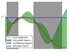
de Freitas et al. (2012) introduced a different GP-based scheme to trade off exploration and exploitation. Instead of optimizing the acquisition function, they proposed to sample the objective function using a finite lattice within a feasible region $R$. The feasible region at the $t^{th}$ iteration is defined as

$$R_{t}=\{\mathbf{x}:\mu_{t}(\mathbf{x})+B_{t}\sigma_{t}{(\mathbf{x})}>\sup_{\mathbf{x}\in R_{t-1}}\mu_{t}(\mathbf{x})-B_{t}\sigma_{t}{(\mathbf{x})}\}.$$

That is, one should only search in the region where the upper bound is greater than the best lower bound encountered thus far, as illustrated in Figure 1. With high probability, the optimizer lies within $R_{t}$.

de Freitas et al. (2012) proved that if we double the density of points in the lattice at each iteration, the feasible region shrinks very quickly. More precisely, they showed that the simple regret vanishes at an exponential rate and that the cumulative regret is bounded by a constant.

With this approach, they did not have to resort to optimizing an acquisition function. However, even in moderate dimensions, their algorithm is impractical since the lattice often becomes too large to be sampled in a reasonable amount of time.

In this paper, we will argue that to overcome this problem, an optimistic strategy may have to be employed. Such a strategy enables us to sample the most promising regions first, so as to avoid the computational cost associated with covering the whole space. In the next section, we begin our discussion of optimistic strategies.

3 Simultaneous optimistic optimization

Algorithm 2 SOO

  Evaluate $f(\mathbf{x}_{0,0})$

  Initialize the tree $\mathcal{T}_{1}=\{0,0\}$

  Set $n=1$

  while true do

     Set $\nu_{\max}=-\infty$

     for $h=0:\min\{\mbox{depth}{({\cal T}_{n}}),h_{\max}(n)\}$ do

        Select $(h,j)=\operatorname*{arg\,max}_{j\in\{j|(h,j)\in L_{n}\}}f(\mathbf{x}_{h,j})$

        if $f(\mathbf{x}_{h,j})>\nu_{\max}$ then

           Evaluate the children of $(h,j)$

           Add the children of $(h,j)$ to ${\cal T}_{n}$

           Set $\nu_{\max}=f(\mathbf{x}_{h,j})$

           Set $n=n+1$

        end if

     end for

  end while

Deterministic optimistic optimization (DOO) and simultaneous optimistic optimization (SOO) are tree-based space partitioning methods for black-box function optimization (Munos, 2011, 2014). They were inspired by the UCT algorithm, which enjoyed great success in planning (Kocsis & Szepesvári, 2006). UCT was shown to have no finite-time guarantees by Coquelin & Munos (2007). This prompted the development of a range of optimistic, in the face of uncertainty, approaches. The term optimism, here, refers to the fact that the strategies expand at each round tree cells that may contain the optimum.

DOO and SOO partition the space ${\cal X}$ hierarchically by building a tree. Let us assume that each node of the tree has $k$ children. A node $(h,j)$ at level $h$ of the tree has children $\{(h+1,kj+i)\}_{0\leq i<k-1}$. The children partition the parent cell $X_{h,j}$ into cells $\{X_{h+1,kj+i},\;0\leq i<k-1\}$. The root cell is the entire space ${\cal X}$. A node is always evaluated at the center of the cell, which we denote as $\mathbf{x}_{h,j}$.

Instead of assuming that the target function is a sample from a GP, DOO and SOO assume the existence of a symmetric semi-metric $\ell$ such that $f(\mathbf{x}^{*})-f(\mathbf{x})\leq\ell(\mathbf{x},\mathbf{x}^{*})$ where $\mathbf{x}^{*}$ is the maximizer of $f$. Although, SOO assumes that $\ell$ exists, it does not require explicit knowledge of it.

DOO on the other hand does require knowledge of $\ell$. DOO builds a tree ${\cal T}_{n}$ incrementally, where $n$ denotes the index over node expansions. DOO expands a leaf $(h,j)$ from the set of leaves $L_{n}$ (nodes whose children are not in ${\cal T}_{n}$) if it has the the highest upper bound: $f(\mathbf{x}_{h,j})+\sup_{\mathbf{x}\in X_{h,j}}\ell(\mathbf{x}_{h,j},\mathbf{x})$. This value for any cell containing $\mathbf{x}^{*}$ upper bounds the best function value $f^{*}$. The performance of DOO depends crucially on our knowledge of the true local smoothness of $f$. SOO aims to overcome the difficulty of having to know the true local smoothness.

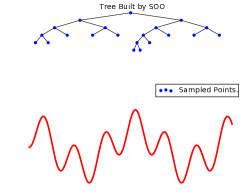
SOO, as summarized in Algorithm 2, expands several leaves simultaneously. When a node is expanded, its children are evaluated. At each round, SOO expands at most one leaf per level, and a leaf is expanded only if it has the largest value among all leaves of the same or lower depths. The SOO algorithm takes as input a function $n\rightarrow h_{\max}(n)$, which limits the maximum height of the tree after $n$ node expansions. $h_{\max}(n)$ defines a tradeoff between deep versus broad exploration. At the end of the finite horizon, SOO returns the $\mathbf{x}$ with the highest objective function value. Figure 2 illustrates the application of SOO to a simple 1-dimensional optimization problem.

Figure 2: [TOP]: The tree built by SOO when optimizing the function $f(x)=\frac{1}{2}\sin(15x)\sin(27x)$ in $[0,1]$. [BOTTOM]: The tree built by BaMSOO. The $20$ blue dots represent nodes where the objective was evaluated. BaMSOO, in comparison, does not evaluate the objective function for points known to be sub-optimal with high probability. Hence, BaMSOO can achieve a better coverage of the search space with the same number of function evaluations as SOO.

4 BaMSOO

SOO offers a different way of trading off exploration and exploitation that does not require the optimization of an acquisition function. However, it does not utilize all the information brought in by the previously evaluated points effectively. To improve upon SOO in practice, we consider the additional assumption that the objective function is a sample from a GP prior.

We define the LCB and UCB to be ${\cal L}_{N}(\mathbf{x}|\mathcal{D}_{t})=\mu(\mathbf{x}|{\cal D}_{t})-B_{N}\sigma(\mathbf{x}|{\cal D}_{t})$ and ${\cal U}_{N}(\mathbf{x}|\mathcal{D}_{t})=\mu(\mathbf{x}|{\cal D}_{t})+B_{N}\sigma(\mathbf{x}|{\cal D}_{t})$ where $B_{N}=\sqrt{2\log(\pi^{2}N^{2}/{6\eta})}$ and $\eta\in(0,1)$.

The BaMSOO algorithm is very similar to SOO. As with SOO, we only evaluate the cell at the center point. However, when a node’s UCB is less than the function value of the best point already sampled, denoted $f^{+}$, we do not evaluate the objective function at this node because with high probability the center point is sub-optimal. Instead, we simply assign to this node its LCB value. Note that if the center-point of a cell is sub-optimal, the cell may still contain the optimizer. Hence this cell must also be further expanded in subsequent iterations. To manage these two types of node in the pseudo-code (see Algorithm 3), we introduce a place-holder function $g$ which is set to $f$ when the UCB of the cell of interest is bigger than $f^{+}$, and it is set to the LCB of the node otherwise. For clarity, we remind the reader that the indices $N,k,t$ and $n$ are over node evaluations, branches (children), function evaluations and node expansions respectively.

In the pseudocode, we have highlighted in blue the additional lines of code brought in by BaMSOO. Effectively, BamSOO only involves a slight modification of SOO (Algorithm 2) provided we have GP routines to evaluate the LCB and UCB.

We found the assignment of the LCB values to nodes that do worse than $f^{+}$ to work well in practice. For this reason our presentation, experiments and theory focus on this choice.

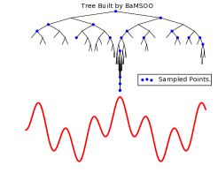
BaMSOO improves upon SOO by making use of the available information more efficiently. Moreover, by using an optimistic proposal, it avoids the need to sample exhaustively before shrinking the feasible region as in (de Freitas et al., 2012). Figure 2 illustrates how BaMSOO can cover the search space more effectively, even though it incurs the same number of expensive function evaluations as SOO.

Algorithm 3 BaMSOO

1:  Set $g_{0,0}=f(\mathbf{x}_{0,0})$

2:  Set $f^{+}=g_{0,0}$

3:  Initialize the tree $\mathcal{T}_{1}=\{0,0\}$

4:  Set $t=1$, $n=1,N=1$, and $\mathcal{D}_{t}=\{(\mathbf{x}_{0,0},g(\mathbf{x}_{0,0}))\}$

5:  while true do

6:     Set $\nu_{\max}=-\infty$.

7:     for $h=0$ to $\min\{\mbox{depth}{({\cal T}_{n}}),h_{\max}(n)\}$ do

8:        Select $(h,j)=\operatorname*{arg\,max}_{j\in\{j|(h,j)\in L_{n}\}}g(\mathbf{x}_{h,j})$

9:        if $g(x_{h,j})>\nu_{\max}$ then

10:           for $i=0$ to $k-1$ do

11:              Set $N=N+1$

12:              if ${\cal U}_{N}(\mathbf{x}_{h+1,kj+i}|\mathcal{D}_{t})\geq f^{+}$ then

13:                 Set $g(\mathbf{x}_{h+1,kj+i})=f(\mathbf{x}_{h+1,kj+i})$

14:                 Set $t=t+1$

15:                 $\mathcal{D}_{t}=\{\mathcal{D}_{t-1},(\mathbf{x}_{h+1,kj+i},g(\mathbf{x}_{h+1,kj+i}))\}$

16:              else

17:                 Set $g(\mathbf{x}_{h+1,kj+i})={\cal L}_{N}(\mathbf{x}_{h+1,kj+i}|\mathcal{D}_{t})$

18:              end if

19:              if $g(\mathbf{x}_{h+1,kj+i})>f^{+}$ then

20:                 Set $f^{+}=g(\mathbf{x}_{h+1,kj+i})$

21:              end if

22:           end for

23:           Add the children of $(h,j)$ to ${\cal T}_{n}$

24:           Set $\nu_{\max}=g(\mathbf{x}_{h,j})$

25:           Set $n=n+1$

26:        end if

27:     end for

28:  end while

5 Analysis

In this section, we provide an overview of the theoretical analysis of BaMSOO, which appears in the Appendix. Our discussion here will focus on our assumptions. At the end of this section, we will present the main result and sketch the proof coarsely.

We denote the global maximum by $f^{*}=\sup_{\mathbf{x}\in{\cal X}}f(\mathbf{x})$ and the maximizer by $\mathbf{x}^{*}=\operatorname*{arg\,max}_{\mathbf{x}\in{\cal X}}f(\mathbf{x})$.

We make similar assumptions to those made by de Freitas et al. (2012). As in their case, we make the global assumption that the objective function is a sample from a GP and a local assumption about the behavior of the objective near the optimum.

Assumption 1 (Conditions on the GP kernel).

${\cal X}\subseteq\mathbb{R}^{D}$ is a compact set, and $\kappa$ is a kernel on $\mathbb{R}^{D}$ that is twice differentiable along the diagonal such that $\partial_{\mathbf{x}}\partial_{\mathbf{x}^{\prime}}\kappa(\mathbf{x},\mathbf{x}^{\prime})|_{\mathbf{x}=\mathbf{x}^{\prime}}$ exists.

Assumption 2 (Local smoothness of $f$).

$f\sim\mbox{GP}(0,\kappa)$ is a continuous sample on ${\cal X}$ that has a unique global maximum $\mathbf{x}^{*}$, such that $f^{*}-c_{1}\|\mathbf{x}-\mathbf{x}^{*}\|^{\alpha}_{2}\leq f(\mathbf{x})$ $\forall\mathbf{x}\in{\cal X}$ and $f(\mathbf{x})\leq f^{*}-c_{2}\|\mathbf{x}-\mathbf{x}^{*}\|^{2}_{2}$ $\forall\mathbf{x}\in{\cal B}(\mathbf{x}^{*},\rho)$ for some constants $c_{1}$, $c_{2}$, $\rho>0$ and $\alpha\in\{1,2\}$. Also $f^{*}-\max_{\mathbf{x}\in{\cal X}\setminus{\cal B}(\mathbf{x}^{*},\rho)}f(\mathbf{x})>\epsilon_{0}$ for some $\epsilon_{0}>0$.

As argued by de Freitas et al. (2012), in many practical cases the local conditions follow almost surely from the global condition. For example, if we were to employ the Matern kernel with $\nu>2$ or a kernel that is $6$ times differentiable along the diagonal, we would have that the samples of the GPs are twice differentiable with probability one. The first case was shown by (Adler & Taylor, 2007, Theorem 1.4.2) and (Stein, 1999, §2.6), while the second result was shown by (Ghosal & Roy, 2006, Theorem 5). If the $\mathbf{x}^{*}$ lies in the interior of ${\cal X}$, then the Hessian of $f$ at $\mathbf{x}^{*}$ would be almost surely non-singular as at least one of the eigenvalues of the Hessian is a co-dimension 1 condition in the space of all functions that are smooth at a given point (de Freitas et al., 2012). In this case, we would have that

$$f^{*}-c_{1}\|\mathbf{x}-\mathbf{x}^{*}\|^{\alpha}_{2}\leq f(\mathbf{x})\leq f^{*}-c_{2}\|\mathbf{x}-\mathbf{x}^{*}\|^{2}_{2}$$

with $\alpha=2$.

If $\mathbf{x}^{*}$ lies on the boundary of ${\cal X}$ which we assume to be smooth, then $\nabla f(\mathbf{x}^{*})\neq 0$ since the additional event of the vanishing of $\nabla f(\mathbf{x}^{*})$ is a co-dimension $d$ phenomenon in the space of functions with global maximum at $\mathbf{x}^{*}$ (de Freitas et al., 2012). In this case, we would have that

$$f^{*}-c_{1}\|\mathbf{x}-\mathbf{x}^{*}\|^{\alpha}_{2}\leq f(\mathbf{x})\leq f^{*}-c_{2}\|\mathbf{x}-\mathbf{x}^{*}\|^{2}_{2}$$

with $\alpha=1$.

Finally, a sample from a GP on a compact domain has a unique maximum with probability one. This is because the space of continuous functions on a compact domain that attain their global maximum at more than one point have co-dimension 1 in the space of all continuous functions on that domain (de Freitas et al., 2012).

The subsequent assumptions are about the hierarchical partitioning of the search space. They are the same as Assumptions 3 and 4 in Munos (2011).

Assumption 3 (Bounded diameters).

There exists a decreasing sequence $\delta(h)>0$, such that for any depth $h\geq 0$, for any cell $X_{h,i}$ of depth $h$, we have $\sup_{\mathbf{x}\in X_{h,i}}\ell(\mathbf{x}_{h,i},\mathbf{x})\leq\delta(h).$ Here $\ell(\mathbf{x},\mathbf{y}):=c_{1}\|\mathbf{x}-\mathbf{y}\|^{\alpha}_{2}$ where $\alpha\in\{1,2\}$ and $\delta(h)=c\gamma^{h}$ for some constant $c>0$ and $\gamma\in(0,1)$.

Assumption 4 (Well-shaped cells).

There exists $\nu>0$ such that for any depth $h\geq 0$, any cell $X_{h,i}$ contains an $\ell$-ball of radius $\nu\delta(h)$ centered in $X_{h,i}$.

Note that depending on the value of $\alpha$, $\gamma$ would have to take on a different value for Assumptions 3 and 4 to be satisfied. Regardless of the choice of $\alpha$ and as illustrated in Example 1 of Bubeck et al. (2011), Assumptions 3 and 4 are easy to satisfy in practice; for example when $\mathbf{x}\in[0,1]^{D}$ and the split is done along the largest dimension of a cell. This is the case in all our experiments.

Assumption 2 together with Assumptions 3 and 4 impose a “near optimality” condition as defined by Munos (2011).

We can now present our main result, which is in the form of a corollary to Theorem 1 in the Appendix.

Corollary 1.

Let $d=-(D/4-D/\alpha)$ and $h_{\max}(n)=n^{\epsilon}$. Given Assumptions $1-4$, we have that with probability at least $1-\eta$, the loss of BaMSOO is $\mathcal{O}\left(n^{-\frac{1-\epsilon}{d}}\log^{\frac{\alpha}{4-\alpha}}(n^{2}/\eta)\right)$.

It is worth pointing out that the result presented in Corollary 1 is based on the number of node expansions $n$ instead of the number of function evaluations. The theory can therefore be strengthened.

If $\alpha=2$ and $\epsilon=1/2$, then the above result translates to $\mathcal{O}\left(n^{-\frac{2}{D}}\log(n^{2}/\eta)\right)$. If $\alpha=1$ with $\epsilon$ being the same as before, then the rate of convergence becomes $\mathcal{O}\left(n^{-\frac{2}{3D}}\log^{\frac{1}{3}}(n^{2}/\eta)\right)$.

The structure of the proof follows that in Munos (2011). Let $\mathbf{x}^{*}_{h}$ denote the optimal node at level $h$ (that is, the node at height $h$ in the branch that contains the optimum $\mathbf{x}^{*}$). Our proof shows that once $\mathbf{x}^{*}_{h}$ is expanded, it does not take long for $\mathbf{x}^{*}_{h+1}$ to be expanded. Once an optimal node $\mathbf{x}^{*}_{h}$ is expanded, by Assumptions 2 and 3, we have that the loss of BaMSOO is no worse than $\delta(h)$ .

The main difficulty of the proof lies in the fact that we sometimes do not sample nodes when their UCB values are less than the best observed value. In this case, we can no longer make the claim that an optimal node is expanded soon after its parent. This is because when a node is not expanded, its LCB can be very low due to a high standard deviation. Fortunately, we can show that this is not the case for optimal nodes in the optimal region. This is accomplished by showing that the standard deviation at a point is no more than its distance to the nearest sampled point up to a constant factor (shown in Lemma 3). This enables us to show that every optimal node in the optimal region must have a low standard deviation. Given this result, we can adopt the proof structure outlined in Munos (2011).

6 Experiments with global optimization benchmarks

Figure 3: Comparison of GP-UCB, SOO, and BaMSOO on multi-modal test functions of low dimensionality (Branin, Rosenbrock and Hartmann3D). GP-UCB and BaMSOO perform similarly whereas SOO does poorly. The poor performance of SOO is caused by having weaker assumptions on the smoothness of the objective function. The good performance of GP-UCB indicates that when the dimensionality is low optimizing the acquisition function is reasonable.

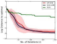
In this section, we validate the proposed algorithm with a series of experiments that compare the three algorithms (GP-UCB, SOO, BaMSOO) on global optimization benchmarks. We have omitted the feasible region shrinking algorithm (described in Section 2.1) as it is not practical for problems of even moderate dimensions. We have also omitted comparisons to PI and EI as these appear in Hoffman et al. (2011) for the optimization benchmarks described in this paper.

In our experiments, we used the same hyper-parameters in GP-UCB and BaMSOO for each test function. We also randomized the initial sample point for BaMSOO and GP-UCB so that they are not deterministic. To optimize the acquisition function for GP-UCB, we used DIRECT followed by a local optimization method using gradients.

We use 5 test functions: Branin, Rosenbrock, Hartmann3, Hartmann6, and Shekel. All of these test functions are common in the global optimization literature and with the exception of the Rosenbrock, they are all multi-modal.

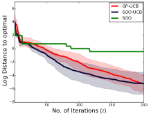
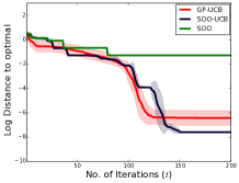
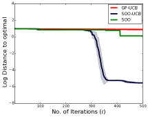
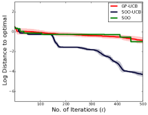
We rescaled the domain of each function to the $[0,1]^{D}$ hypercube, and we used the log distance to the true optimum as our evaluation metric. This metric is defined as $\log_{10}(f^{*}-f^{+})$ where $f^{+}$ is the best objective value sampled so far and $f^{*}$ is the true maximum value of the objective. For each test function, we repeat our experiments $50$ times for GP-UCB and BaMSOO and run SOO once as SOO is a deterministic strategy. We plot the mean and a confidence bound of one standard deviation of our metric across all the runs for all the tests.

Figure 4: Comparison of GP-UCB, SOO, and BaMSOO on multi-modal test functions of moderate dimensionality: 4D Shekel function (top) and 6D Hartmann function (bottom). Here, GP-UCB performs poorly. This is due in part to the hardness of optimizing the acquisition function.

Table 1: Time required for the test functions measured in seconds. SOO is very fast as it does not maintain a GP. BaMSOO maintains a GP to produce more accurate posterior estimates and is hence slower. The rejection of proposals also results in bigger trees, further slowing down the algorithm. GP-UCB is slow compared to the other two algorithms as it not only maintains a GP but also optimizes its acquisition function at each iteration.

Algorithm	Branin	Rosenbrock	Hartmann3	Hartmann6	Shekel
GP-UCB	29.9438	29.5716	34.0311	115.2402	100.7770
BaMSOO	3.0680	3.4693	3.9722	2.0918	3.8951
SOO	0.1810	0.1835	0.1871	0.4313	0.4350

For simplicity, we only consider binary-trees for space partitioning in SOO and BaMSOO. Specifically, the largest dimension in the parent’s cell is split to create two children.

First, we test the global optimization schemes on $3$ test functions with low dimensionality: Branin, Rosenbrock and Hartmann3. The Branin function (Jones, 2001) is a common benchmark for Bayesian optimization and has 2 dimensions. The Rosenbrock function is a commonly used non-convex test function for local optimization algorithms, and although it is unimodal, its optimum lies in a long narrow valley, which makes the function hard to optimize. Finally, the Hartmann3 function is $3$-dimensional and has four local optima.

As we can see from Figure 3, BaMSOO performs competitively against GP-UCB on these low dimensional test functions. Both BaMSOO and GP-UCB achieve very high accuracies of up to $10^{-8}$ in terms of the distance to the optimal objective value. In comparison, SOO, due to the lack of a strong prior assumption, cannot take advantage of the points sampled and thus is lagging behind.

In the experiments shown in Figure 4, we compare the approaches in consideration on the Shekel function and the Hartmann6 function. The Shekel function is 4-dimensional and has 10 local optima. The Hartmann6 function is 6-dimensional, as the name suggests, and has 6 local optima. On these higher dimensional problems, the performance of GP-UCB begins to dwindle. Despite the increase in dimensionality, BaMSOO is still able to optimize the test functions to a relatively high precision. SOO does not perform as well as BaMSOO again because of its weak assumptions. The poor performance of GP-UCB on these two test functions may be due in part to the inability of a global optimizer to optimize the acquisition function exactly in each iteration. As the dimensionality increases, so is the difficulty of optimizing a non-convex function globally as the cost of covering the space grows exponentially. The optimization of the acquisition function through algorithms like DIRECT demands the repartitioning of the space in each iteration. To reach a finer granularity, we either have to sacrifice speed by building very fine partitions in each iteration or accuracy by using coarser partitions.

The proposed approach is not only competitive with GP-UCB in terms of effectiveness, it is also more computationally efficient. As we can see in Table 1, BaMSOO is about 10-40 times faster than GP-UCB on the test functions that we have experimented with. This is because instead of optimizing the acquisition function in each iteration the SOO algorithm, that sits inside, only optimizes once. BaMSOO, however, is much slower than SOO. This is because BaMSOO also employs a GP to reject points proposed by SOO. To sample one point, SOO may have to propose many points before one is accepted. For this reason, BaMSOO would build much bigger trees compared to SOO and it is therefore slower.

7 Application to term extraction

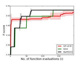
In this section, we evaluate the performance of the BaMSOO algorithm on optimizing the parameters in a term extraction algorithm. Term extraction is the process of analyzing a text corpus to find terms, where terms correspond to cohesive sequences of words describing entities of interest. Term extraction tools are widely used in industrial text mining and play a fundamental role in the construction of knowledge graphs and semantic search products. Recently Parameswaran et al. (2010) proposed a term extraction method, and showed that it outperforms state-of-the-art competitors, but their method has many free parameters that require manual adjustment. Here, we compare the performance of BaMSOO, GP-UCB and SOO in automatically tuning the 4 primary free parameters of the algorithm (support-thresholds). We define our deterministic objective function to be the F-score of the extracted terms, which is a weighted average of precision and recall. Precision is calculated using a predefined set of correct terms and recall is estimated by simply normalizing the number of extracted correct terms to be in the range [0,1]. We run the experiment on the GENIA corpus (Kim et al., 2003), which is a collection of 2000 abstracts from biomedical articles. The results of the experiment are shown in Figure 5. It is evident from this figure that BaMSOO outperforms GP-UCB and SOO in this application.

Figure 5: Comparison of GP-UCB, SOO, and BaMSOO on optimizing 4 parameters in term extraction from the GENIA corpus using a term extraction algorithm by (Parameswaran et al., 2010). In this plot, higher is better.

8 Discussion

This paper introduced a new global optimization algorithm BaMSOO, which does not require the auxiliary optimization of either acquisition functions or samples from the GP. In trials with benchmark functions from the global optimization literature, the new algorithm outperforms standard BO with GPs and SOO, while being computationally efficient. The paper also provided a theoretical analysis proving that the loss of BaMSOO decreases polynomially.

The careful reader may have noticed that, despite the effectiveness of BaMSOO in the experiments, the convergence rate of BaMSOO is not as good as that of SOO for $\alpha=2$. This is because we were only able to prove that the standard deviation at a point decreases linearly, instead of quadratically, when a nearby point is sampled (Lemma 3 in the Appendix). Since by assumption the objective function behaves quadratically in the optimal region, the linear decrease of the standard deviation gives rise to a sub-optimal convergence rate. It is also interesting to note that the same type of bound on the standard deviation was used by Bull (2011), who achieved similar convergence rates to the ones in this paper. de Freitas et al. (2012) showed that if the samples form a $\delta$-cover on a subset of ${\cal D}\subseteq{\cal X}$, then the standard deviation of all points on ${\cal D}$ is bounded by a quadratic term $\frac{Q}{4}\delta^{2}$. Via this observation, the authors achieved a geometric convergence rate. The requirement of the $\delta$-cover, however, renders their algorithm impractical. Finding a practical GP-based algorithm that achieves geometric convergence rates remains an open problem.

Appendix A Proofs

We begin by introducing some notation. Let $\mathbf{x}^{*}_{h}$ denote the optimal node at level $h$. That is the cell of $\mathbf{x}^{*}_{h}$ contains the optimizer $\mathbf{x}^{*}$. Also let $f^{+}$ and $\mathbf{x}^{+}$ represent the best function value observed thus far and the associated node respectively.

A.1 Technical Lemmas

Lemma 1 (Lemma 5 of de Freitas et al. (2012)).

Given a set of points $\mathbf{x}_{1:T}:=\{\mathbf{x}_{1},\ldots,\mathbf{x}_{T}\}\in\mathcal{D}$ and a Reproducing Kernel Hilbert Space (RKHS) ${\cal H}$ with kernel $\kappa$ the following bounds hold:

1. Any $f\in{\cal H}$ is Lipschitz continuous with constant $\|f\|_{\cal H}L$, where $\|\cdot\|_{\cal H}$ is the Hilbert space norm and $L$ satisfies the following:

   $$L^{2}\leq\sup_{\mathbf{x}\in\mathcal{D}}\partial_{\mathbf{x}}\partial_{\mathbf{x}^{\prime}}\kappa(x,x^{\prime})|_{\mathbf{x}=\mathbf{x}^{\prime}}$$

   and for $\kappa(\mathbf{x},\mathbf{x}^{\prime})=\widetilde{\kappa}(\mathbf{x}-\mathbf{x}^{\prime})$ we have

   $$L^{2}\leq\partial_{\mathbf{x}}^{2}\widetilde{\kappa}(\mathbf{x})|_{x=0}.$$

2. The projection operator $P_{1:T}$ on the subspace $\displaystyle\operatorname*{span}_{t=1:T}\{\kappa(x_{t},\cdot)\}\subseteq{\cal H}$ is given by

   $$P_{1:T}f:=\mathbf{k}^{\top}(\cdot)\mathbf{K}^{-1}\left<\mathbf{k}(\cdot),f\right>$$

   where $\mathbf{k}(\cdot)=\mathbf{k}_{1:T}(\cdot):=\left[\kappa(\mathbf{x}_{1},\cdot)\cdots\kappa(\mathbf{x}_{T},\cdot)\right]^{\top}$ and $\mathbf{K}:=\left[\kappa(\mathbf{x}_{i},\mathbf{x}_{j})\right]_{i,j=1:T}$; moreover, we have that

   $$\left<\mathbf{k}(\cdot),f\right>:=\begin{bmatrix}\left<\kappa(\mathbf{x}_{1},\cdot),f\right>\\ \vdots\\ \left<\kappa(\mathbf{x}_{T},\cdot),f\right>\end{bmatrix}=\begin{bmatrix}f(\mathbf{x}_{1})\\ \vdots\\ f(\mathbf{x}_{T})\end{bmatrix}.$$

   Here $P_{1:T}P_{1:T}=P_{1:T}$ and $\|P_{1:T}\|\leq 1$ and $\|\operatorname*{\mathbf{1}}-P_{1:T}\|\leq 1$.

3. Given tuples $(\mathbf{x}_{i},f_{i})$ with $f_{i}=f(\mathbf{x}_{i})$, the minimum norm interpolation $\bar{f}$ with $\bar{f}(\mathbf{x}_{i})=f(\mathbf{x}_{i})$ is given by $\bar{f}=P_{1:T}f$. Consequently its residual $g:=(\mathbf{1}-P_{1:T})f$ satisfies $g(\mathbf{x}_{i})=0$ for all $\mathbf{x}_{i}\in\mathbf{x}_{1:T}$.

Lemma 2 (Lemma 6 of de Freitas et al. (2012)).

Under the assumptions of Lemma 1 it follows that

$$|f(\mathbf{x})-P_{1:T}f(\mathbf{x})|\leq\|f\|_{\cal H}\sigma_{T}(\mathbf{x}),$$

where $\sigma_{T}^{2}(\mathbf{x})=\kappa(\mathbf{x},\mathbf{x})-\mathbf{k}_{1:T}^{\top}(\mathbf{x})\mathbf{K}^{-1}\mathbf{k}_{1:T}(\mathbf{x})$ and this bound is tight. Moreover, $\sigma_{T}^{2}(\mathbf{x})$ is the posterior predictive variance of a Gaussian process with the same kernel.

Lemma 3 (Adapted from Proposition 1 of de Freitas et al. (2012)).

Let $\kappa:\mathbb{R}^{D}\times\mathbb{R}^{D}\to\mathbb{R}$ be a kernel that is twice differentiable along the diagonal $\{(\mathbf{x},\mathbf{x})\,|\,\mathbf{x}\in\mathbb{R}^{D}\}$, with $L$ defined as in Lemma 1.1, and $f$ be an element of the RKHS with kernel $\kappa$. If $f$ is evaluated at point $\mathbf{x}$, then for any other point $\mathbf{y}$ we have $\sigma_{T}(\mathbf{y})\leq L\|\mathbf{x}-\mathbf{y}\|$.

Proof.

Let ${\cal H}$ be the RKHS corresponding to $\kappa$ and $f\in{\cal H}$ an arbitrary element with $g:=(\operatorname*{\mathbf{1}}-P_{1:T})f$; the residual defined in lemma 1.3. Since $g\in{\cal H}$, we have by Lemma 1.1, $g$ is Lipschitz. Thus we have that for any point $\mathbf{y}$:

$$|g(\mathbf{y})|\leq L\|g\|_{{\cal H}}\|\mathbf{y}-\mathbf{x}\|\leq L\|f\|_{{\cal H}}\|\mathbf{y}-\mathbf{x}\|,$$ (2)

where the second inequality is guaranteed by Lemma 1.2. On the other hand, by Lemma 2, we know that for all $\mathbf{y}$ we have the following tight bound:

$$|g(\mathbf{y})|\leq\|f\|_{{\cal H}}\sigma_{T}(\mathbf{y})$$ (3)

Now, given the fact that both inequalities (2) and (3) are bounding the same quantity and that the latter is a tight estimate, we necessarily have that:

$$\|f\|_{{\cal H}}\sigma_{T}(\mathbf{y})\leq L\|f\|_{{\cal H}}\|\mathbf{y}-\mathbf{x}\|.$$

Canceling $\|f\|_{{\cal H}}$ gives us the result. ∎

Lemma 4 (Adapted from Lemma 5.1 of Srinivas et al. (2010)).

Let $f$ be a sample from a GP. Consider $\eta\in(0,1)$ and set $B_{T}=2\log(\pi_{T}/\eta)$ where $\sum_{i=1}^{\infty}\pi_{T}^{-1}=1$, $\pi_{T}>0$. Then,

$$|f(\mathbf{x}_{T})-\mu_{T}(\mathbf{x}_{T})|\leq B_{T}^{\frac{1}{2}}\sigma_{T}(\mathbf{x}_{T})\mbox{ }\forall T\geq 1$$

holds with probability at least $1-\eta$.

Proof.

For $\mathbf{x}_{T}$ we have that $f(\mathbf{x})\sim{\cal N}(\mu_{T}(\mathbf{x}_{T}),\sigma_{T}(\mathbf{x}_{T}))$ since $f$ is a sample from the GP. Now, if $r\sim{\cal N}(0,1)$, then

$$\mathbb{P}(r>c) = e^{-c^{2}/2}(2\pi)^{-1/2}\int e^{-(r-c)^{2}/2-c(r-c)}dr$$

$$< e^{-c^{2}/2}\mathbb{P}(r>0)=\frac{1}{2}e^{-c^{2}/2}.$$

Thus we have that

$$\mathbb{P}\left(f(\mathbf{x})-\mu_{T}(\mathbf{x})>B_{T}^{1/2}\sigma_{T}(\mathbf{x})\right)=\mathbb{P}(r>B_{T}^{1/2})<\frac{1}{2}e^{-B_{T}/2}.$$

By symmetry and the union bound, we have that $\mathbb{P}\left(|f(\mathbf{x})-\mu_{T}(\mathbf{x})|>B_{T}^{1/2}\sigma_{T}(\mathbf{x})\right)<e^{-B_{T}/2}.$ By applying the union bound again, we derive

$$\mathbb{P}\left(|f(\mathbf{x})-\mu_{T}(\mathbf{x})|>B_{T}^{1/2}\sigma_{T}(\mathbf{x})\mbox{ }\forall T\geq 1\right)<\sum_{T=1}^{\infty}e^{-B_{T}/2}.$$

By substituting $B_{T}=2\log(\pi_{T}/\eta)$, we obtain the result. As in Srinivas et al. (2010), we can set $\pi_{T}=\pi^{2}T^{2}/6$. ∎

Since each node’s UCB and LCB are only evaluated at most once, we give the following shorthands in notation. Let $N(\mathbf{x})$ be the number of evaluations of confidence bounds by the time the UCB of $\mathbf{x}$ is evaluated (line 12 of Algorithm 3) and let $T(\mathbf{x})=|{\cal D}_{t}|$ be the time the UCB of $\mathbf{x}$ is evaluated. Define $\mathcal{U}(\mathbf{x})={\cal U}_{N(\mathbf{x})}(\mathbf{x}|\mathcal{D}_{T(\mathbf{x})})=\mu(\mathbf{x}|{\cal D}_{T(\mathbf{x})})+B_{N(\mathbf{x})}\sigma(\mathbf{x}|{\cal D}_{T(\mathbf{x})})$ and $\mathcal{L}(\mathbf{x})={\cal L}_{N(\mathbf{x})}(\mathbf{x}|\mathcal{D}_{T(\mathbf{x})})=\mu(\mathbf{x}|{\cal D}_{T(\mathbf{x})})-B_{N(\mathbf{x})}\sigma(\mathbf{x}|{\cal D}_{T(\mathbf{x})})$.

Lemma 5.

Consider ${\cal B}(\mathbf{x}^{*},\rho)$ and $\gamma in(0,1)$ as in Assumptions 2 and 3. Suppose ${\cal L}(\mathbf{x}^{*}_{h})\leq f(\mathbf{x}^{*}_{h})\leq\mathcal{U}(\mathbf{x}^{*}_{h})$. If $\mathbf{x}_{h}^{*}\in{\cal B}(\mathbf{x}^{*},\rho)$ and $\delta(h)<\epsilon_{0}$ then there exists a constant $\bar{c}$ such that ${\cal L}(\mathbf{x}_{h}^{*})\geq f^{*}-\bar{c}B_{{N(\mathbf{x}^{*}_{h})}}\gamma^{\frac{h}{2}}$.

Proof.

If $\mathbf{x}_{h}^{*}$ is not evaluated then $f(\mathbf{x}^{+})\geq\mathcal{U}_{T}(\mathbf{x}_{h}^{*})\geq f^{*}-\delta(h)\geq f^{*}-\epsilon_{0}$ which implies that $\mathbf{x}^{+}\in{\cal B}(\mathbf{x}^{*},\rho)$. Therefore, $f^{*}-c_{2}\|\mathbf{x}^{+}-\mathbf{x}^{*}\|^{2}\geq f(\mathbf{x}^{+})\geq\mathcal{U}_{T}(\mathbf{x}_{h}^{*})\geq f^{*}-\delta(h)$ which in turn implies that $\|\mathbf{x}^{+}-\mathbf{x}^{*}\|\leq\sqrt{\frac{\delta(h)}{c_{2}}}$. Similarly $f^{*}-c_{2}\|\mathbf{x}_{h}^{*}-\mathbf{x}^{*}\|^{2}\geq f(\mathbf{x}_{h}^{*})\geq f^{*}-\delta(h)$. Therefore $\|\mathbf{x}_{h}^{*}-\mathbf{x}^{*}\|\leq\sqrt{\frac{\delta(h)}{c_{2}}}$. By the triangle inequality, we have

$$\|\mathbf{x}^{+}-\mathbf{x}_{h}^{*}\|\leq\|\mathbf{x}^{+}-\mathbf{x}^{*}\|+\|\mathbf{x}_{h}^{*}-\mathbf{x}^{*}\|\leq 2\sqrt{\frac{\delta(h)}{c_{2}}}.$$

By Lemma 3, we have that $\sigma_{T(\mathbf{x}^{*}_{h})}(\mathbf{x}^{*}_{h})\leq 2L\sqrt{\frac{\delta(h)}{c_{2}}}$. By the definition of ${\cal L}_{T}$, we can argue that

$${\cal L}(\mathbf{x}^{*}_{h}) \geq \mathcal{U}(\mathbf{x}_{h}^{*})-4B_{{N(\mathbf{x}^{*}_{h})}}L\sqrt{\frac{\delta(h)}{c_{2}}}$$

$$\geq f^{*}-\delta(h)-4B_{{N(\mathbf{x}^{*}_{h})}}L\sqrt{\frac{\delta(h)}{c_{2}}}$$

$$= f^{*}-c\gamma^{h}-4B_{{N(\mathbf{x}^{*}_{h})}}L\sqrt{\frac{c\gamma^{h}}{c_{2}}}.$$

Note that since $\gamma\in(0,1)$, $\gamma<\gamma^{1/2}$. Assume that $B_{1}=b$. Let $\bar{c}=c/b+4L\sqrt{\frac{c}{c_{2}}}$. Since $B_{N}>B_{1}$ $\forall N>1$, we have the statement.

If $\mathbf{x}_{h}^{*}$ is evaluated then the statement is trivially true. ∎

Definition 1.

Let $\bar{\gamma}:=\gamma^{\frac{1}{2}}$, $\bar{\delta}_{h}:=\bar{c}B_{N(\mathbf{x}^{*}_{h})}\bar{\gamma}^{h}$, and $I_{h}^{\epsilon}=\{(h,i):f(\mathbf{x}_{h,i})+\epsilon\geq f^{*}\}$.

Lemma 6.

Assume that $h_{\max}=n^{\epsilon}$. For a node $\mathbf{x}_{h,i}$ at level $h$, $B_{N(\mathbf{x}_{h,i})}=\mathcal{O}(\sqrt{h})$.

Proof.

Assume that there are $n_{i}$ nodes expanded at the end of iteration $i$ of the outer loop (the while loop). In the $i+1^{th}$ iteration of the outer loop, there can be at most $h_{\max}(n_{i})$ additional expansions added. Thus the total number of expansions at the end of iteration $i$ is at most $n_{i-1}+h_{\max}(n_{i-1})$. We can prove by induction that $n_{i}\leq i^{\frac{1}{1-\epsilon}}$. Since any node at level $h$ would be expanded after at most $2^{h}$ iterations, at the time of expansion of any node at level $h$, we have that $n<(2^{h})^{\frac{1}{1-\epsilon}}=2^{\frac{h}{1-\epsilon}}$ where $n$ is the total number of expansions. Thus, there would be at most $2\times 2^{\frac{h}{1-\epsilon}}$ evaluations. Hence,

$$B_{N(\mathbf{x}_{h,i})}\leq\sqrt{2\log(\pi^{2}2^{\frac{2h}{1-\epsilon}+2}/{6\eta})}\leq\sqrt{2\log(2^{\frac{2h}{1-\epsilon}+2})+2\log(\pi^{2}/{6\eta)}}=\mathcal{O}(\sqrt{h}).$$

∎

Lemma 7.

After a finite number of node expansions, an optimal node $\mathbf{x}_{h_{0}}^{*}\in{\cal B}(\mathbf{x}^{*},\rho)$ is expanded such that $\bar{c}B_{N(\mathbf{x}_{h_{0}}^{*})}\bar{\gamma}^{h}_{0}\leq\epsilon_{0}$. Also $\forall h>h_{0}$, we have that $\bar{c}B_{N(\mathbf{x}^{*}_{h})}\bar{\gamma}^{h}\leq\epsilon_{0}$ and $\mathbf{x}_{h}^{*}\in{\cal B}(\mathbf{x}^{*},\rho)$.

Proof.

Since it is clear that BaMSOO would expand every node after a finite number of node expansions, we only have to show that there exists an $h_{0}$ that satisfies the conditions. By Lemma 6, we have that $\forall h$ $B_{N(\mathbf{x}^{*}_{h})}=\mathcal{O}(\sqrt{h})$. Since $\bar{\gamma}<1$, there exists an $h_{0}$ such that $\bar{c}B_{N(\mathbf{x}^{*}_{h})}\bar{\gamma}^{h}\leq\epsilon_{0}$ $\forall h>h_{0}$. Since $f(\mathbf{x}^{*}_{h})>f^{*}-\delta(h)>f^{*}-\bar{c}B_{N(\mathbf{x}^{*}_{h})}\bar{\gamma}^{h}\geq f^{*}-\epsilon_{0}$, we have by Assumption 2 that, $\mathbf{x}^{*}_{h}\in{\cal B}(\mathbf{x}^{*},\rho)$. ∎

Lemma 8.

$\sum_{h=0}^{H}|I_{h}^{\bar{\delta}(H)}|\leq C\left(B_{N\left(\mathbf{x}^{*}_{H}\right)}\right)^{D/2}\gamma^{(D/4-D/\alpha)H}$ for some constant $C$ for all $H>h_{0}$.

Proof.

By Lemma 7, we know that $\bar{\delta}(H)=\bar{c}B_{N(\mathbf{x}^{*}_{H})}\bar{\gamma}^{H}<\epsilon_{0}$ if $H>h_{0}$. Therefore, by Assumption 2, we have that $\chi_{\bar{\delta}(H)}=\{\mathbf{x}\in\chi:f(\mathbf{x})\geq f^{*}-\bar{\delta}(H)\}\subseteq{\cal B}(x^{*},\rho).$ Again by Assumption 2, we have that

$$f^{*}-\bar{\delta}(H)\leq f(\mathbf{x})\leq f^{*}-c_{2}\|\mathbf{x}-\mathbf{x}^{*}\|^{2}_{2}\mbox{ }\forall\mathbf{x}\in\chi_{\bar{\delta}(H)}.$$

Thus $\chi_{\bar{\delta}(H)}\subseteq{\cal B}\left(x^{*},\sqrt{\frac{\bar{\delta}(H)}{c_{2}}}\right)={\cal B}\left(x^{*},\sqrt{\frac{\bar{c}B_{N\left(\mathbf{x}^{*}_{H}\right)}\gamma^{H/2}}{c_{2}}}\right)$.

Since each cell $(h,i)$ contains a $\ell$-ball of radius $\nu\delta(h)$ centered at $\mathbf{x}_{h,i}$ we have that each cell contains a ball ${\cal B}(\mathbf{x}_{h,i},(\nu\delta(h))^{1/\alpha})={\cal B}(\mathbf{x}_{h,i},(\frac{\nu c}{c_{1}})^{1/\alpha}\gamma^{h/\alpha})$. By the argument of volume, we have that $|I_{h}^{\bar{\delta}(H)}|\leq C_{1}\left(B_{N\left(\mathbf{x}^{*}_{H}\right)}\right)^{D/2}\gamma^{HD/4-hD/\alpha}$ for some constant $C_{1}$. Finally,

$$\sum_{h=0}^{H}|I_{h}^{\bar{\delta}(H)}| \leq C_{1}\sum_{h=0}^{H}\left(B_{N\left(\mathbf{x}^{*}_{H}\right)}\right)^{D/2}\gamma^{HD/4-hD/\alpha}$$

$$= C_{1}\left(B_{N\left(\mathbf{x}^{*}_{H}\right)}\right)^{D/2}\gamma^{HD/4}\sum_{h=0}^{H}\gamma^{-hD/\alpha}$$

$$= C_{1}\left(B_{N\left(\mathbf{x}^{*}_{H}\right)}\right)^{D/2}\gamma^{HD/4}\sum_{h=0}^{H}\left(\gamma^{D/\alpha}\right)^{h-H}$$

$$\leq C_{1}\left(B_{N\left(\mathbf{x}^{*}_{H}\right)}\right)^{D/2}\gamma^{HD/4}\sum_{h=0}^{\infty}\left(\gamma^{D/\alpha}\right)^{h-H}$$

$$= C_{1}\left(B_{N\left(\mathbf{x}^{*}_{H}\right)}\right)^{D/2}\gamma^{HD/4}\frac{\gamma^{-DH/\alpha}}{1-\gamma^{D/\alpha}}$$

$$= \frac{C_{1}}{1-\gamma^{D/\alpha}}\left(B_{N\left(\mathbf{x}^{*}_{H}\right)}\right)^{D/2}\gamma^{HD/4-DH/\alpha}$$

$$= \frac{C_{1}}{1-\gamma^{D/\alpha}}\left(B_{N\left(\mathbf{x}^{*}_{H}\right)}\right)^{D/2}\gamma^{(D/4-D/\alpha)H}.$$

Setting $C=\frac{C_{1}}{1-\gamma^{D/\alpha}}$ gives us the desired result. ∎

Lemma 9.

Suppose ${\cal L}(\mathbf{x}^{*}_{h})\leq f(\mathbf{x}^{*}_{h})\leq\mathcal{U}(\mathbf{x}^{*}_{h})$. If $\mathbf{x}_{h}^{*}$ is not evaluated (that is $\mathcal{U}(\mathbf{x}^{*}_{h})<f^{+}$) then $f^{+}$ is $\delta(h)$-optimal.

Proof.

$f^{+}>\mathcal{U}(\mathbf{x}^{*}_{h})\geq f(\mathbf{x}^{*}_{h})>f^{*}-\delta(h).$ ∎

A.2 Main Results

A.2.1 Simple Regret

Let $h^{*}_{n}$ be the deepest level of an expanded optimal node with $n$ node expansions. This following lemma is adapted from Lemma 2 of Munos (2011).

Lemma 10.

Suppose ${\cal L}(\mathbf{x})\leq f(\mathbf{x})\leq\mathcal{U}(\mathbf{x})$ for all $\mathbf{x}$ whose confidence region are evaluated. Whenever $h\leq h_{\max}(n)$ and $n\geq Ch_{\max}(n)\sum_{i=h_{0}}^{h}\left(B_{N\left(\mathbf{x}^{*}_{i}\right)}\right)^{D/2}\gamma^{(D/4-D/\alpha)i}+n_{0}$ for some constant $C$, we have $h^{*}_{n}\geq h$.

Proof.

We prove the statement by induction. By Lemma 7, we have that after $n_{0}$ node expansions, a node $\mathbf{x}_{h_{0}}^{*}\in{\cal B}(\mathbf{x}^{*},\rho)$ is expanded. Also $\forall h>h_{0}$, we have that $\bar{c}B_{N(\mathbf{x}^{*}_{h})}\bar{\gamma}^{h}\leq\epsilon_{0}$ and $\mathbf{x}_{h}^{*}\in{\cal B}(\mathbf{x}^{*},\rho)$. For $h=h_{0}$, the statement is trivially satisfied. Thus assume that the statement is true for $h$. Let n be such that $n\geq Ch_{\max}(n)\sum_{i=h_{0}}^{h+1}\left(B_{N\left(\mathbf{x}^{*}_{i}\right)}\right)^{D/2}\gamma^{(D/4-D/\alpha)i}+n_{0}$. By the inductive hypothesis we have that $h_{n}^{*}\geq h$. Assume $h_{n}^{*}=h$ since otherwise the proof is finished. As long as the optimal node at level $h+1$ is not expanded, all nodes expanded at the level are $\bar{\delta}(h+1)$-optimal by Lemma 5. By Lemma 8, we know that after $Ch_{\max}(n)\left(B_{N\left(\mathbf{x}^{*}_{h+1}\right)}\right)^{D/2}\gamma^{(D/4-D/\alpha)(h+1)}$ node expansions, the optimal node at level $h+1$ will be expanded since there are at most $\sum_{i=0}^{h+1}\left|I_{i}^{\bar{\delta}(h+1)}\right|$ $\bar{\delta}(h+1)$-optimal nodes at or beneath level $h+1$. Thus $h_{n}^{*}\geq h+1$. ∎

Theorem 1.

Suppose ${\cal L}(\mathbf{x})\leq f(\mathbf{x})\leq\mathcal{U}(\mathbf{x})$ for all $\mathbf{x}$ whose confidence region is evaluated. Let us write $h(n)$ to be the smallest integer $h\geq h_{0}$ such that

$$Ch_{\max}(n)\sum_{i=h_{0}}^{h}\left(B_{N\left(\mathbf{x}^{*}_{i}\right)}\right)^{D/2}\gamma^{(D/4-D/\alpha)i}+n_{0}\geq n.$$

Then the loss is bounded as

$$r_{n}\leq\delta(\min\{h(n),h_{\max}(n)+1\})$$

and $h_{n}^{*}\geq\min\{h(n)-1,h_{\max}(n)\}$.

Proof.

From Lemma 8, and the definition of $h(n)$ we have that

$$Ch_{\max}(n)\sum_{i=h_{0}}^{h(n)-1}\left(B_{N\left(\mathbf{x}^{*}_{i}\right)}\right)^{D/2}\gamma^{(D/4-D/\alpha)i}+n_{0}<n.$$

By Lemma 10, we have that $h_{n}^{*}\geq h(n)-1$ if $h(n)-1\leq h_{\max}(n)$ and $h_{n}^{*}\geq h_{\max}(n)$ otherwise. Therefore $h_{n}^{*}\geq\min\{h(n)-1,h_{\max}(n)\}$.

By Lemma 9, we know that if $\mathbf{x}_{h_{n}^{*}+1}^{*}$ is not evaluated then $f^{+}$ is $\delta(h_{n}^{*}+1)$-optimal. If $\mathbf{x}_{h_{n}^{*}+1}^{*}$ is evaluated, then $f\left(\mathbf{x}_{h_{n}^{*}+1}^{*}\right)$ is $\delta(h_{n}^{*}+1)$-optimal. Thus $r_{n}\leq\delta(\min\{h(n),h_{\max}(n)+1\}).$ ∎

Proof of Corollary 1.

Suppose ${\cal L}(\mathbf{x})\leq f(\mathbf{x})\leq\mathcal{U}(\mathbf{x})$ for all $\mathbf{x}$ whose confidence region is evaluated. By Lemma 4, we know that this holds with probability at least $1-\eta$.

By the definition of $h(n)$ we have that

$$n \leq Ch_{\max}(n)\sum_{i=h_{0}}^{h(n)}\left(B_{N\left(\mathbf{x}^{*}_{i}\right)}\right)^{D/2}\gamma^{(D/4-D/\alpha)i}+n_{0}$$ (4)

$$\leq Ch_{\max}(n)\left(B_{N\left(\mathbf{x}_{h(n)}^{*}\right)}\right)^{D/2}\sum_{i=h_{0}}^{h(n)}\gamma^{-di}+n_{0}$$

$$\leq Ch_{\max}(n)\left(B_{N\left(\mathbf{x}_{h(n)}^{*}\right)}\right)^{D/2}\gamma^{-dh_{0}}\frac{\gamma^{-dh(n)}-1}{\gamma^{-d}-1}+n_{0}$$

If $h(n)\leq h_{\max}(n)+1$, then by Theorem 1, we have that $h_{n}^{*}\geq h(n)-1$. After $n$ expansions, the optimal node $\mathbf{x}_{h(n)-1}^{*}$ has been expanded which suggests that its children’s confidence bounds have been evaluated. Hence, $N\left(\mathbf{x}_{h(n)}^{*}\right)<2n$ since there have only been $n$ expansions. Therefore,

$$(\ref{no5})\leq Kn^{\epsilon}\left(B_{2n}\right)^{D/2}\gamma^{-dh(n)}$$

for some constant $K$ which implies that

$$\gamma^{h(n)}\leq K^{1/d}B_{2n}^{\frac{2\alpha}{4-\alpha}}n^{-\frac{1-\epsilon}{d}}=K^{1/d}\left[2\log(4\pi^{2}n^{2}/{6\eta})\right]^{\frac{\alpha}{4-\alpha}}n^{-\frac{1-\epsilon}{d}}.$$

By Theorem 1, we have that

$$r_{n}\leq c\min\left\{K^{1/d}\left[2\log(4\pi^{2}n^{2}/{6\eta})\right]^{\frac{\alpha}{4-\alpha}}n^{-\frac{1-\epsilon}{d}},\gamma^{(n+1)^{\epsilon}}\right\}=\mathcal{O}\left(n^{-\frac{1-\epsilon}{d}}\log^{\frac{\alpha}{4-\alpha}}(n^{2}/\eta)\right).$$

∎

References

- Adler & Taylor (2007) Adler, R. J. and Taylor, J. E. Random Fields and Geometry. Springer, 2007.
- Agrawal & Goyal (2013) Agrawal, S. and Goyal, N. Thompson sampling for contextual bandits with linear payoffs. In International Conference on Machine Learning, 2013.
- Bardenet & Kégl (2010) Bardenet, R. and Kégl, B. Surrogating the surrogate: accelerating Gaussian-process-based global optimization with a mixture cross-entropy algorithm. In International Conference on Machine Learning, pp. 55–62, 2010.
- Bergstra et al. (2011) Bergstra, J., Bardenet, R., Bengio, Y., and Kégl, B. Algorithms for hyper-parameter optimization. In Advances in Neural Information Processing Systems, pp. 2546–2554, 2011.
- Brochu et al. (2007) Brochu, E., de Freitas, N., and Ghosh, A. Active preference learning with discrete choice data. In Advances in Neural Information Processing Systems, pp. 409–416, 2007.
- Brochu et al. (2009) Brochu, E., Cora, V. M., and de Freitas, N. A tutorial on Bayesian optimization of expensive cost functions, with application to active user modeling and hierarchical reinforcement learning. Technical Report UBC TR-2009-23 and arXiv:1012.2599v1, Dept. of Computer Science, University of British Columbia, 2009.
- Brochu et al. (2010) Brochu, E., Brochu, T., and de Freitas, N. A Bayesian interactive optimization approach to procedural animation design. In Proceedings of the 2010 ACM SIGGRAPH/Eurographics Symposium on Computer Animation, pp. 103–112, 2010.
- Bubeck et al. (2011) Bubeck, S., Munos, R., Stoltz, G., and Szepesvari, C. X-armed bandits. Journal of Machine Learning Research, 12:1655–1695, 2011.
- Bull (2011) Bull, A. D. Convergence rates of efficient global optimization algorithms. Journal of Machine Learning Research, 12:2879–2904, 2011.
- Chen et al. (2012) Chen, B., Castro, R.M., and Krause, A. Joint optimization and variable selection of high-dimensional Gaussian processes. In International Conference on Machine Learning, 2012.
- Coquelin & Munos (2007) Coquelin, P.A. and Munos, R. Bandit algorithms for tree search. In Uncertainty in Artificial Intelligence, pp. 67–74, 2007.
- de Freitas et al. (2012) de Freitas, N., Smola, A., and Zoghi, M. Exponential regret bounds for Gaussian process bandits with deterministic observations. In International Conference on Machine Learning, 2012.
- Garnett et al. (2010) Garnett, R., Osborne, M. A., and Roberts, S. J. Bayesian optimization for sensor set selection. In ACM/IEEE International Conference on Information Processing in Sensor Networks, pp. 209–219. ACM, 2010.
- Ghosal & Roy (2006) Ghosal, S. and Roy, A. Posterior consistency of Gaussian process prior for nonparametric binary regression. The Annals of Statistics, 34:2413–2429, 2006.
- Hansen & Ostermeier (2001) Hansen, N. and Ostermeier, A. Completely derandomized self-adaptation in evolution strategies. Evol. Comput., 9(2):159–195, 2001.
- Hennig & Schuler (2012) Hennig, P. and Schuler, C.J. Entropy search for information-efficient global optimization. The Journal of Machine Learning Research, 98888:1809–1837, 2012.
- Hoffman et al. (2009) Hoffman, M., Kueck, H., de Freitas, N., and Doucet, A. New inference strategies for solving Markov decision processes using reversible jump MCMC. In Uncertainty in Artificial Intelligence, pp. 223–231, 2009.
- Hoffman et al. (2011) Hoffman, M., Brochu, E., and de Freitas, N. Portfolio allocation for Bayesian optimization. In Uncertainty in Artificial Intelligence, pp. 327–336, 2011.
- Hoffman et al. (2014) Hoffman, M.W., Shahriari, B., and de Freitas, N. On correlation and budget constraints in model-based multi-armed-bandit optimization with application to automatic machine learning. In AI and Statistics, 2014.
- Hutter et al. (2011) Hutter, F., Hoos, H. H., and Leyton-Brown, K. Sequential model-based optimization for general algorithm configuration. In Proceedings of LION-5, pp. 507 523, 2011.
- Jones et al. (1993) Jones, D. R., Perttunen, C. D., and Stuckman, B. E. Lipschitzian optimization without the Lipschitz constant. Journal of Optimization Theory and Applications, 79(1):157–181, 1993.
- Jones (2001) Jones, D.R. A taxonomy of global optimization methods based on response surfaces. J. of Global Optimization, 21(4):345–383, 2001.
- Kaufmann et al. (2012) Kaufmann, E., Korda, N., and Munos, R. Thompson sampling: An asymptotically optimal finite-time analysis. In Algorithmic Learning Theory, volume 7568 of Lecture Notes in Computer Science, pp. 199–213. Springer Berlin Heidelberg, 2012.
- Kim et al. (2003) Kim, J., Ohta, T., Tateisi, Y., and ichi Tsujii, J. GENIA corpus - a semantically annotated corpus for bio-textmining. In ISMB (Supplement of Bioinformatics), pp. 180–182, 2003.
- Kocsis & Szepesvári (2006) Kocsis, L. and Szepesvári, C. Bandit based Monte-Carlo planning. In European Conference on Machine Learning, pp. 282–293. 2006.
- Kueck et al. (2006) Kueck, H., de Freitas, N., and Doucet, A. SMC samplers for Bayesian optimal nonlinear design. In IEEE Nonlinear Statistical Signal Processing Workshop, pp. 99–102, 2006.
- Kueck et al. (2009) Kueck, H., Hoffman, M., Doucet, A., and de Freitas, N. Inference and learning for active sensing, experimental design and control. In Araujo, H., Mendonca, A., Pinho, A., and Torres, M. (eds.), Pattern Recognition and Image Analysis, volume 5524, pp. 1–10. Springer Berlin Heidelberg, 2009.
- Lizotte et al. (2011) Lizotte, D., Greiner, R., and Schuurmans, D. An experimental methodology for response surface optimization methods. J. of Global Optimization, pp. 1–38, 2011.
- Mahendran et al. (2012) Mahendran, N., Wang, Z., Hamze, F., and de Freitas, N. Adaptive MCMC with Bayesian optimization. Journal of Machine Learning Research - Proceedings Track, 22:751–760, 2012.
- Martinez-Cantin et al. (2007) Martinez-Cantin, R., de Freitas, N., Doucet, A., and Castellanos, J. A. Active policy learning for robot planning and exploration under uncertainty. Robotics Science and Systems, 2007.
- May et al. (2011) May, B. C., Korda, N., Lee, A., and Leslie, D. S. Optimistic Bayesian sampling in contextual bandit problems. Technical Report 11:01, Statistics Group, School of Mathematics, University of Bristol, 2011.
- Močkus (1982) Močkus, J. The Bayesian approach to global optimization. In Systems Modeling and Optimization, volume 38, pp. 473–481. Springer, 1982.
- Munos (2011) Munos, R. Optimistic optimization of a deterministic function without the knowledge of its smoothness. In Advances in Neural Information Processing Systems, pp. 783–791, 2011.
- Munos (2014) Munos, R. From Bandits to Monte-Carlo Tree Search: The Optimistic Principle Applied to Optimization and Planning. Technical Report hal-00747575, INRIA Lille, 2014.
- Parameswaran et al. (2010) Parameswaran, A., Garcia-Molina, H., and Rajaraman, A. Towards the web of concepts: Extracting concepts from large datasets. Proceedings of the VLDB Endowment, 3(1-2):566–577, 2010.
- Rasmussen & Williams (2006) Rasmussen, C. E. and Williams, C. K. I. Gaussian Processes for Machine Learning. The MIT Press, 2006.
- Snoek et al. (2012) Snoek, J., Larochelle, H., and Adams, R. P. Practical Bayesian optimization of machine learning algorithms. In Advances in Neural Information Processing Systems, 2012.
- Srinivas et al. (2010) Srinivas, N., Krause, A., Kakade, S. M., and Seeger, M. Gaussian process optimization in the bandit setting: No regret and experimental design. In International Conference on Machine Learning, pp. 1015–1022, 2010.
- Stein (1999) Stein, M. L. Interpolation of Spatial Data: Some Theory for Kriging. Springer, 1999.
- Valko et al. (2013) Valko, M., Carpentier, A., and Munos, R. Stochastic simultaneous optimistic optimization. In International Conference on Machine Learning, 2013.
- Vazquez & Bect (2010) Vazquez, E. and Bect, J. Convergence properties of the expected improvement algorithm with fixed mean and covariance functions. J. of Statistical Planning and Inference, 140:3088–3095, 2010.
- Wang et al. (2013) Wang, Z., Zoghi, M., Matheson, D., Hutter, F., and de Freitas, N. Bayesian optimization in high dimensions via random embeddings. In International Joint Conference on Artificial Intelligence, 2013.