Abstract

Targeted therapies based on biomarker profiling are becoming a mainstream direction of cancer research and treatment. Depending on the expression of specific prognostic biomarkers, targeted therapies assign different cancer drugs to subgroups of patients even if they are diagnosed with the same type of cancer by traditional means, such as tumor location. For example, Herceptin is only indicated for the subgroup of patients with HER2+ breast cancer, but not other types of breast cancer. However, subgroups like HER2+ breast cancer with effective targeted therapies are rare and most cancer drugs are still being applied to large patient populations that include many patients who might not respond or benefit. Also, the response to targeted agents in human is usually unpredictable. To address these issues, we propose SUBA, subgroup-based adaptive designs that simultaneously search for prognostic subgroups and allocate patients adaptively to the best subgroup-specific treatments throughout the course of the trial. The main features of SUBA include the continuous reclassification of patient subgroups based on a random partition model and the adaptive allocation of patients to the best treatment arm based on posterior predictive probabilities. We compare the SUBA design with three alternative designs including equal randomization, outcome-adaptive randomization and a design based on a probit regression. In simulation studies we find that SUBA compares favorably against the alternatives.

KEY WORDS: Adaptive designs; Bayesisan inference; Biomarkers; Posterior; Subgroup identification; Targeted therapies.

1 Introduction

1.1 Targeted Therapy

With the rapid development in genomics and personalized medicine it is becoming increasingly more feasible to diagnose and treat cancer based on measurements from genomic interrogations at the molecular level such as gene expression (Van De Vijver et al., 2002; Snijders et al., 2001), DNA copy numbers (Curtis et al., 2012; Baladandayuthapani et al., 2010), and epigenetic marks (Wang et al., 2008; Barski and Zhao, 2009; Mitra et al., 2013). In particular, pairing genetic traits with targeted treatment options has been an important focus in recent research. This has led to successful findings such as the use of trastuzumab, doxorubicin, or taxanes on HER2+ breast cancer (Hudis, 2007), and the recommendation against treatment with EGFR antibodies on KRAS mutated colorectal cancer (Misale et al., 2012). It is now broadly understood that patients with the same cancer defined by classification criteria such as tumor location, staging, and risk-stratification can respond differently to the same drug, depending on their genetic profiling.

First proposed by Simon and Maitournam (2004), “targeted designs” restrict the eligibility of patients to receive a treatment based on predicted response using genomic information. Under fixed sample sizes and comparing to standard equal randomization with two-arm trials, the authors showed that targeted designs could drastically increase the study power in situations where the new treatment benefited only a subset of patients and those patients could be accurately identified. Sargent et al. (2005) proposed the biomarker-by-treatment interaction design and a biomarker-based-strategy design, both using prognostic biomarkers to facilitate treatment allocations to targeted subgroups. Maitournam and Simon (2005) further showed that the relative efficiency of target designs depended on (1) the relative sizes of the treatment effects in biomarker positive and negative subgroups, (2) the prevalence of the patient group who favorably responds to the experimental treatment, and (3) the accuracy of the biomarker evaluation. Recently, new designs have been proposed by Freidlin et al. (2010), Simon (2010) and Mandrekar and Sargent (2010), among others.

BATTLE (Kim et al., 2011) and I-SPY 2 (Barker et al., 2009) are two widely known biomarker cancer trials using Bayesian designs. The design of BATTLE predefined five biomarker groups on the basis of 11 biomarkers, and assigned patients to four drugs using an outcome-adaptive randomization (AR) scheme. AR is implemented with the expectation that an overall higher response rate would be achieved relative to equal randomization (ER), assuming at least one biomarker group has variations in the outcome distributions across arms. However, the analysis of the trial data revealed otherwise; the response rate was actually slightly lower during the AR period than during the initial ER period. This fact can be attributed to several factors such as possible trends in the enrolled population, or variations in the procedures for measuring primary outcomes. In practice, targeted agents can fail for reasons such as having no efficacy on the targeted patients, being unexpectedly toxic, or uniformly ineffective. There is a need for adaptive designs to accommodate the situations above to improve trial efficiency and maintain trial ethic (Yin et al., 2012; Gu and Lee, 2010; Zhu et al., 2013).

Researchers are also developing new designs that allow for the redefinition of biomarker groups that could be truly responsive to targeted treatments. Ruberg et al. (2010) and Foster et al. (2011) developed tree-based algorithms to identify and evaluate the subgroup effects by searching the covariate space for regions with substantially better treatment effects. Bayesian models are natural candidates for adaptive learning of subgroups, and have been known and applied in non-medical contexts (Loredo, 2003; Kruschke, 2008).

1.2 A Subgroup-Based Adaptive Design

In this paper, we propose a class of SUbgroup-Based Adaptive (SUBA) designs for targeted therapies which utilize individual biomarker profiles and clinical outcomes as they become available.

To understand and characterize a clinical trial design it is useful to distinguish between the patients in the trial versus future patients. There exist a number of methods that address the optimization for the patients in the trial. Most approaches are targeting the optimization of a pre-selected objective function (criterion). See, for example, (Fedorov and Leonov, 2013, chapters 8 and 9). SUBA aims to address both goals, successful treatment of patients in the trial and optimizing treatment selection for future patients. We achieve the earlier by allocating each patient on the basis of the patient’s biomarker profile $\bm{x}$ to the treatment with the best currently estimated success probability. That is, the optimal treatment $t^{\ast}$ for a patient with biomarker profile $\bm{x}$ is

$$t^{\ast}(\bm{x})=\arg\max_{t\in\Omega}\hat{\theta}_{t}(\bm{x}),$$

where $\hat{\theta}_{t}(\bm{x})$ is the posterior predictive response rate of a patient with biomarker profile $\bm{x}$ under treatment $t$. This can be characterized as a stochastic optimization problem. In contrast, the optimal treatment selection for future patients is not considered as an explicit criterion in SUBA. It is indirectly addressed by partitioning the biomarker space into subsets with different response probabilities for the treatments under consideration. Learning about the implied patient subpopulations facilitates personalized treatment selection for a future patient on the basis of the patient’s biomarker profile $\bm{x}$. The outcome of SUBA is an estimated partition of the biomarker space and the corresponding optimal treatment assignments.

The main assumption underlying the proposed design approach is that there exist subgroups of patients who differentially respond to treatments. For example, consider a scenario with two subgroups of patients that respond well to either of two different treatments, but not both. An ideal design should search for such subgroups and link each subgroup with its corresponding superior treatment. That is, a design should aim to identify subgroups with elevated response rates to particular treatments. The key innovations of SUBA are that such biomarker subgroups are continuously redefined based on patients’ differential responses to treatments and that patients are allocated to the currently estimated best treatment based on posterior predictive inference.

In summary, SUBA conducts subgroup discovery, estimation, and patient allocation simultaneously. We propose a prior for the partition that classifies tumor profiles into biomarker subgroups. The stochastic partition has the advantage that biomarker subgroups are not fixed up front before patients accrual. The goal is to use the data, during the trial, to learn which partitions are likely to be relevant and could potentially become clinically useful. We define a random partition of tumor profiles using a tree-based model that shares similarities with Bayesian CART algorithms (Chipman et al., 1998; Denison et al., 1998). We provide closed-form expressions for posterior computations and describe an algorithm for adaptive patient allocation during the course of the trial.

1.3 Motivating Trial

We consider a breast cancer trial with three candidate treatments. Patients who are eligible have undergone neoadjuvant systemic therapy (NST) and surgery. Protein biomarkers for all patients are measured through biopsy samples by reverse phase protein arrays (RPPA) at the end of NST, but before surgery. The first treatment is a poly (ADP-ribose) polymerase (PARP) inhibitor, which affects DNA repair and cell death programming. The second treatment is a PI3K pathway inhibitor, which affects cell growth, proliferation, cell differentiation and ultimate survival. The third treatment is a cell cycle inhibitor that targets the cell cycle pathway. The main goal is to identify for each of the three treatments subgroups of patients that will respond favorably to the respective treatment.

The paper proceeds as follows. Section 2 presents the probability model of SUBA design and computation details for implementing the design. Section 3 examines the operating characteristics based on simulation studies. We conclude with a brief discussion in Section 4.

2 Methodology

2.1 Sampling Model

Assume that $T$ candidate treatments are under consideration in a clinical trial. We use $t\in\Omega=\{1,\ldots,T\}$ to index the treatments and $i=1,\ldots,N$ to index patients. We assume a maximum sample size of $N$ patients. The primary outcome for each patient is a binary variable $y_{i}\in\{0,1\}$. We assume that $y_{i}$ can be measured without delay. We denote with $\bm{x}_{i}=(x_{i2},\dots,x_{iK})^{\prime}$ the biomarker profile of the $i$-th patient, recorded at baseline. We assume that all biomarkers $x_{ik}$ are continous, $x_{ik}\in\mathbb{R}$. Finally, let $z_{i}$ denote the treatment allocation for patient $i$ with $z_{i}=t$ if patient $i$ is assigned to treatment $t$.

The underlying assumption of a biomarker clinical trial is that there exist subgroups of patients that differentially respond to the same treatment. For example, subgroup $1$ may respond well to treatment $t_{1}$ but not $t_{2}$ while subgroup $2$ may respond well to treatment $t_{2}$ but not $t_{1}$. However, the subgroups are not known before the trial and must be estimated adaptively based on response data and biomarker measurements from already treated patients. To estimate the subgroups and their expected response rates to treatments, we propose a random partition model. Assuming that all $K$ biomarker measurements are continuous, $x_{ik}\in\mathbb{R}$, we construct patient subgroups by defining a partition of the biomarker space $\mathbb{R}^{K}$. A partition is a family of subsets $\Pi=\{S_{1},S_{2},\dots,S_{M}\}$, where $M$ is the size of the partition and $S_{m}$ are the partitioning subsets such that $S_{m}\cap S_{l}=\emptyset$ and $\cup_{m}S_{m}=\mathbb{R}^{K}$. The partition of the biomarker sample space implies a partition of the patients into biomarker subgroups. Patient $i$ belongs to biomarker subgroup $m$ if $\bm{x}_{i}\in S_{m}$. We will construct a prior probability measure for $\Pi$ in the next section. In the following discussion we will occasionally refer to $S_{m}$ as a subset of patients, implying the subset of patients that is defined by the partitioning subset $S_{m}$.

We define a sampling model for $y_{i}$ conditional on $\bm{x}_{i}$ and $\Pi$ as

$$p(y_{i}=1\mid z_{i}=t,\Pi,\bm{x}_{i}\in S_{m})=\theta_{t,m},$$ (1)

where $\theta_{t,m}$ is the response rate of treatment $t$ for a patient in subgroup $S_{m}$. Thus the joint likelihood function for $n$ patients is the product of $n$ such Bernoulli probabilities, using $\theta_{t,m}$ and $(1-\theta_{t,m})$ depending on the recorded outcomes $y_{i}$. In each biomarker subgroup $S_{m}$, let $n_{m}=\sum_{i}I(\bm{x}_{i}\in S_{m})$ count the number of patients, $n_{mt}=\sum_{i}I(\bm{x}_{i}\in S_{m},\;z_{i}=t)$ the number of patients assigned to treatment $t$, and $n_{mty}=\sum_{i}I(\bm{x}_{i}\in S_{m},\;z_{i}=t,\;y_{i}=y)$ the number of patients in group $m$ assigned to $t$ with response $y_{i}=y$. Here $I(\cdot)$ is the indicator function. Let $\bm{y}^{(n)}=(y_{1},\dots,y_{n})^{\prime}$, $\bm{X}^{(n)}=\{\bm{x}_{i}\}_{i=1}^{n}$, $\bm{z}^{(n)}=(z_{1},\dots,z_{n})^{\prime}$, and $\bm{\theta}=\{\theta_{t,m};\;t=1,\ldots,T,\;m=1,\ldots,M\}$. Then

$$p(\bm{y}^{(n)}\mid\bm{X}^{(n)},\bm{z}^{(n)},\bm{\theta},\Pi_{r})=\prod_{m}\prod_{t}\theta_{t,m}^{n_{mt1}}(1-\theta_{t,m})^{n_{mt0}}.$$

Adding a prior on $\Pi$ and $\bm{\theta}$ we complete (1) to define a 3-level hierarchical model

$$p(\bm{y}^{(n)},\bm{\theta},\Pi\mid\bm{X}^{(n)},\bm{z}^{(n)})\propto p(\bm{y}^{(n)}\mid\bm{X}^{(n)},\bm{z}^{(n)},\bm{\theta},\Pi)\,p(\bm{\theta}\mid\Pi)\,p(\Pi).$$ (2)

The last two factors define the prior model for $\bm{\theta}$ and $\Pi$. We assume $\theta_{t,m}\mid\Pi\stackrel{{\scriptstyle i.i.d}}{{\sim}}\mathrm{Beta}(a,b)$ and discuss the prior for $\Pi$ next. Posterior inference on $\Pi$ and $\bm{\theta}$ provides learning on subgroups and their treatment-specific response rates. Posterior probabilities for $\Pi$ and $\bm{\theta}$ are the key inference summaries that we will later use to define the desired adaptive trial design.

2.2 Random Biomarker Partition $\Pi$

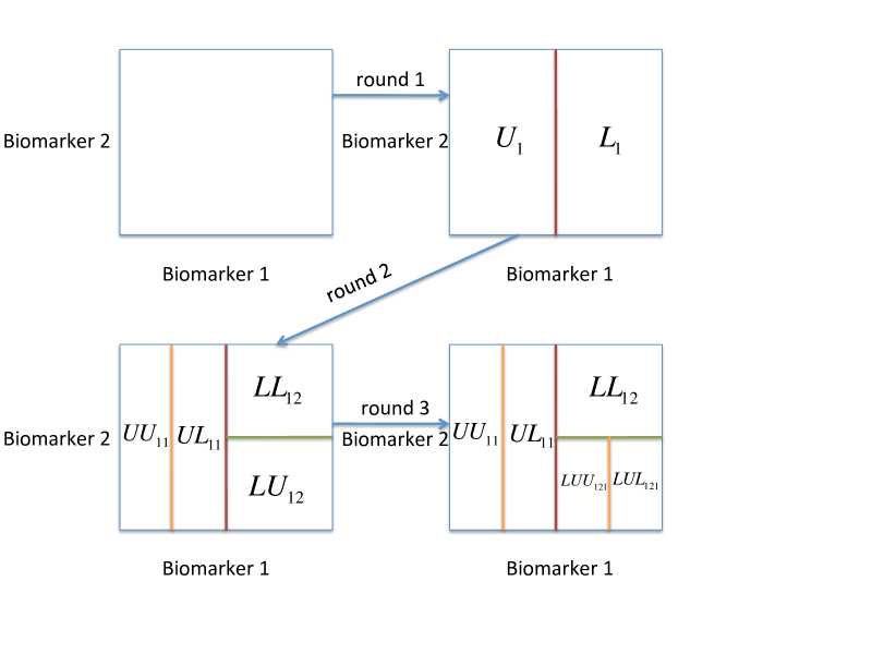
We propose a tree-type random partition $\Pi$ on the biomarker space $\mathbb{R}^{K}$ to define random biomarker subgroups. A partition is obtained through a tree of recursive binary splits. Each node of the tree corresponds to a subset of $\mathbb{R}^{K}$, and is either a final leaf which defines one of the partioning subsets $S_{m}$, or it is in turn split into two descendants. In the latter case the two descendants are defined by first selecting a biomarker $k$ and then splitting the current subset by thresholding $x_{ik}$. The threshold splits the ancestor set into two components. A sequence of such splits generates a partition of $\mathbb{R}^{K}$ as the collection of the resulting subsets. For the motivating breast cancer trial, we limit the partition to at most eight biomarker subgroups in the random partition. We impose this constraint to limit the number of subgroups with critically small numbers of patients, and therefore only allow three rounds of random splits.

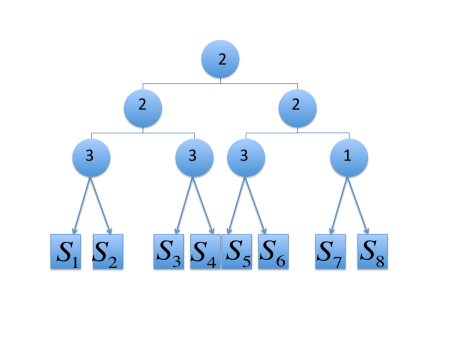
An example is shown in Figure 1. The figure shows a realization of the random partition with $K=2$ biomarkers. In each round, we consider each of the current subsets and either do not split it further with probability $v_{0}$ or with probability $v_{k}$ choose biomarker $k$ to split the subset into two parts. If an ancestor subset $S$ is split by the $k$-th biomarker, then the resulting partition contains two new subsets, defined by $\{i:x_{ik}\geq med_{k}(S)\}$ and $\{i:x_{ik}<med_{k}(S)\}$, where $med_{k}(S)$ is the median of $x_{ik}$ and is computed across all available data points in the subset $S$. That is, $med_{k}(S)$ is a conditional median which can vary during the course of the trial, as more data become available. In Figure 1 the sequence of splits is as follows. We first split on $x_{i1}$. In the second round the two resulting subsets are split on $x_{i1}$ and $x_{i2}$, respectively. In a third round of splits, only one subset of the earlier four subsets is split on $x_{i1}$ again, three others are not further split.

Let $\bm{\Pi}$ be the sample space of all possible partitions based on the three rounds of splits. For each partition $\Pi\in\bm{\Pi}$, we calculate the prior probability $p(\Pi_{r})$ based on the above random splitting rules. For example, the partition $\Pi$ in Figure 1 has prior probability

$$p(\Pi)\propto v_{1}\times v_{1}\,v_{2}\times v_{0}\,v_{0}\,v_{0}\,v_{1},$$ (3)

with the three factors corresponding to the three rounds of splits.

We use a variation of the described probability model. The main rational is that, if a biomarker is selected for an initial split, then it is desirable to augment the probability of splitting it again at the subsequent levels in the tree. The goal is to facilitate the identification of relevant subgroups maintaining the simplicity of the partition model. To implement this, in each possible partition $\Pi$, we calculate $K$ as the number of distinct biomarkers selected in the three rounds of splits. We then add an additional penalty term proportional to $\phi^{K}$ to the above prior probability of $\Pi$, so that the prior favors partitions that repeatedly split on the same marker. For example, in Figure 1, the modified prior probability is

$$p(\Pi)\propto v_{1}^{3}\,v_{2}\,v_{0}^{3}\times\phi^{2}.$$ (4)

Similarly, we can calculate the prior probability for any partition $\Pi$ in $\bm{\Pi}$. When $\phi=1$ the two probability models that we described coincide while values of $\phi$ in $(0,1)$ allow one to tune the concentration of over partitions that split over a parsimonious number of biomarkers.

2.3 Decision Rule for Patient Allocation

A major objective of the SUBA design is to assign future patients to superior treatments based on their biomarker profiles and the observed outcomes of all previous patients. Assuming that the outcomes of the first $n$ patients have been observed, we denote by $q(t,\bm{x}_{n+1})$ the posterior predictive probability of response under treatment $t$ for an $(n+1)^{th}$ patient with biomarker profile $\bm{x}_{n+1}$. Denoting the observed trial data $\mathcal{D}_{n}=\{\bm{y}^{(n)},\bm{X}^{(n)},\bm{z}^{(n)}\}$, based on (2),

$$q(t,\bm{x}_{n+1})\equiv p(y_{n+1}=1\mid\bm{x}_{n+1},z_{n+1}=t,\mathcal{D}_{n})\\ =\sum_{\Pi_{r}\in\bm{\Pi}}p(y_{n+1}=1\mid\bm{x}_{n+1},z_{n+1}=t,\Pi_{r},\mathcal{D}_{n})\;p(\Pi_{r}\mid\mathcal{D}_{n}).$$ (5)

The posterior probability $p(\Pi_{r}\mid\mathcal{D}_{n})$ can be computed as follows. Given a partition $\Pi_{r}=(S_{1},\dots,S_{M_{r}})\in\bm{\Pi}$, all $n$ patients are divided into $M_{r}$ biomarker subgroups. Recall the definition of $n_{m},n_{mt}$ and $n_{mty}$ from Section 2.1. The posterior distribution of $\Pi_{r}$ is

$$p(\Pi_{r}\mid\mathcal{D}_{n})\propto p(\Pi_{r})\,p(\mathcal{D}_{n}\mid\Pi_{r})=p(\Pi_{r})\,\prod_{m}\prod_{t}\left\{\int\prod_{\bm{x}_{i}\in S_{m}}p(y_{i}\mid\bm{x}_{i},z_{i}=t,\theta_{t,m})\;dp(\theta_{t,m})\right\},$$

where $p(\Pi_{r})$ is the prior probability of partition $\Pi_{r}$ that can be calculated as in (4). Let $B(a,b)=\Gamma(a)\Gamma(b)/\Gamma(a+b)$ denote the beta function, and let $\mbox{Be}(x;\,a,b)\propto x^{a-1}(1-x)^{b-1}$ denote a beta p.d.f. With independent $\mbox{Be}(x;\,a,b)$ prior distributions for the $\theta_{t,m}$ parameters we can further simplify the above equation to

$$p(\Pi_{r}\mid\mathcal{D}_{n})\propto p(\Pi_{r})\,\prod_{m}\prod_{t}\left\{\int\theta_{t,m}^{n_{mt1}}(1-\theta_{t,m})^{n_{mt0}}\;\mbox{Be}(\theta_{t,m};\,a,b)~{}d\theta_{t,m}\right\}\,=\\ =p(\Pi_{r})\;\prod_{m}\prod_{t}\frac{B(a+n_{mt1},b+n_{mt0})}{B(a,b)}.$$ (6)

The conditional probability $p(y_{n+1}=1\mid\bm{x}_{n+1},z_{n+1}=t,\Pi,\mathcal{D}_{n})$ is the integral of (1) with respect to the $\mbox{Be}(a+n_{mt1},b+n_{mt0})$ posterior on $\theta_{t,m}$. Then

$$p(y_{n+1}=1\mid\bm{x}_{n+1},z_{n+1}=t,\Pi_{r},\mathcal{D}_{n}) = \sum_{m}I(\bm{x}_{n+1}\in S_{m})\int\theta_{t,m}\,dp(\theta_{t,m}\mid\Pi_{r},\mathcal{D}_{n})$$ (7)

$$= \sum_{m}I(\bm{x}_{n+1}\in S_{m})\frac{a+n_{mt1}}{a+b+n_{mt}}.$$

Let $m(\bm{x}_{n+1},\Pi)$ index the partitioning subset with $\bm{x}_{n+1}\in S_{m(\bm{x}_{n+1},\Pi)}$. The sum over $m$ in (7) reduces to just the term with $m=m(\bm{x}_{n+1},\Pi)$. Combining (6) and (7), we compute the posterior predictive response rate of $(n+1)^{th}$ patient receiving treatment $t$ in closed form

$$q(t,\bm{x}_{n+1})=\sum_{\Pi_{r}\in\bm{\Pi}}p(y_{n+1}=1\mid\bm{x}_{n+1},z_{n+1}=t,\Pi_{r},\mathcal{D}_{n})\;p(\Pi_{r}\mid\mathcal{D}_{n}).$$ (8)

Denote with $z^{\star}_{n+1}\in\Omega$ the treatment decision for the $(n+1)^{th}$ patient. We choose $z^{\star}_{n+1}$ by adopting a minimum posterior predictive loss approach described in Gelfand and Ghosh (1998). Under a variety of loss functions (such as the 0-1 loss), the optimal rule that minimizes the posterior predictive loss is

$$z^{\star}_{n+1}=\arg\max_{t\in\Omega}\;q(t,\bm{x}_{n+1}).$$ (9)

See Raiffa and Schlaifer (1961) or Gelfand and Ghosh (1998) for details. Alternatively, one could use the probabilities $q(t,\bm{x}_{n+1})$ in a biased randomization $p(z^{\star}_{n+1}=t)\propto q(t,\bm{x}_{n+1})^{c}$, as proposed in Thall and Wathen (2007).

2.4 The SUBA Design

Computing the posterior predictive response rates for all candidate treatments allows us to compare treatments and monitor the trial accordingly. If one treatment is inferior to all other treatments, that treatment should be dropped from the trial. If there is only one treatment left after dropping inferior treatments, the trial should be stopped early due to ethical and logistics reasons.

The SUBA design starts a trial with a run-in phase during which patients are equally randomized to treatments. After the initial run-in, we continuously monitor the trial until either the trial is stopped early based on a stopping rule, or the trial is stopped after reaching a prespecified maximum sample size $N$.

We include rules to exclude inferior treatments and stop the trial early if indicated. Recall that the biomarker space is $\mathbb{R}^{K}$. Consider the $k$-th biomarker and observed biomarker values $\{x_{1k},\ldots,x_{nk}\}$. We define an equally spaced grid of size $H_{0}$ between $\min_{k}$ and $\max_{k}$, where $\min_{k}$ and $\max_{k}$ are the observed smallest and largest values for that biomarker. Taking the Cartesian product of these grids we then create a $K-$dimensional grid $\tilde{\bm{x}}$ of size $H=H_{0}^{K}$. Let $\tilde{x}_{h}\in\mathbb{R}^{K}$, $h=1,\ldots,H$, denote the list of all grid points. After an initial run-in phase with equal randomization, we evaluate the posterior predictive response rate $q(t,\tilde{x}_{h})$ for treatment $t$ for each $\tilde{x}_{h}$. Any treatment $t^{\star}$ with uniformly inferior success probability

$$q(t^{*},\tilde{x}_{h})<q(t,\tilde{x}_{h}),\mbox{ for all }h=1,\ldots,H\mbox{ and }t\neq t^{\star}$$

is dropped from the trial. That is, we remove $t^{\star}$ from the list of treatments, $\Omega\equiv\Omega\setminus\{t^{\star}\}$. Also, if only one treatment is left in the trial, then the trial is stopped early.

Alternatively to the construction of the grid $\tilde{\bm{x}}$, any available data set of typical biomarker values $\tilde{x}_{h}\in\mathbb{R}^{K}$ could be used. For large $K$ this is clearly preferable. If such data were available, it could also be used for an alternative definition of $med_{k}$ in the specification of the splits in the prior for $\Pi_{r}$ discussed earlier.

The SUBA design consists of the following steps.

1. Initial run-in. Start the trial and randomize $n<N$ patients equally to $T$ treatments in the set $\Omega$. 2. Treatment exclusion and early stopping. Drop treatment $t^{*}$ if $q(t^{*},\tilde{x}_{h})<q(t,\tilde{x}_{h})$ for all $t\neq t^{*}$ and $h=1,\ldots,H$. Set $\Omega=\Omega\setminus\{t^{*}\}$. If enrollment remains active only for a single treatment $t$ then stop the trial. 3. Adaptive patient allocation. Allocate patient $(n+1)$ to treatment $z^{\star}_{n+1}$ according to (9). When the response $y_{n+1}$ is available, go back to step 2 and repeat for patients $n+2,n+3,\dots,N$. 4. Reporting patient subpopulations. Upon conclusion of the trial we report the estimated partition $\Pi$ together with the estimated optimal treatment allocations.

In step 4, summarizing the posterior distribution over random partitions and determining the best partition over a large number of possible partitions $\Pi$ is a challenging problem. Following Medvedovic et al. (2004) we define an $(N\times N)$ association matrix $G^{\Pi_{r}}$ of co-clustering indicators for each partition $\Pi_{r}$. Here $G^{\Pi_{r}}_{ij}$ is an indicator of patients $i$ and $j$ being in the same subgroup with respect to the biomarker partition $\Pi_{r}$. Dahl (2006) introduced a least-squares estimate for random partitions using draws from Markov chain Monte Carlo (MCMC) posterior simulation. Following their idea, we propose a least-square summary

$$\Pi^{LS}=\arg min_{\Pi_{r}}||G^{\Pi_{r}}-\hat{G}||^{2},$$

where $\hat{G}=\sum_{r}G^{\Pi_{r}}p(\Pi_{r}\mid\mathcal{D}_{n})$ is the posterior mean association matrix and $||A||^{2}$ denotes the sum of squared elements of a matrix $A$. In words, $\Pi^{LS}$ minimizes the sum of squared deviations of between an association matrix $G^{\Pi_{r}}$ and the posterior mean $\hat{G}$.

Alternatively one could report a partition that minimizes the average squared deviation, averaging with respect to $p(\Pi_{r}\mid\mathcal{D})$. That is, minimize posterior mean squared distance instead of squared distance to the posterior mean association matrix. While the earlier has an appealing justification as a formal Bays rule, the latter is easier to compute.

3 Simulation Studies

3.1 Simulation Setup

We conduct simulation studies to evaluate the proposed design. The setup is chosen to mimic the motivating breast cancer study. For each simulated trial, we fix a maximum sample size of $N=300$ patients in a three-arm study with three treatments $t=1,2,3$. We assume that a set of $K=4$ biomarkers are measured at baseline for each patient and generate $x_{ik}$ from a uniform distribution on $[-1,1]$, i.e., $x_{ik}\sim\mbox{Unif}\ (-1,1)$. The hyperprior parameters are fixed as $v_{k}=1/(K+1)$, $k=0,1,\dots,K$, $\phi=0.5$, $a=1$ and $b=1$. That is, each biomarker has the same prior probability of being selected for a split, and the response rates $\theta_{t,m}$ have uniform priors. To set up the grid $\tilde{\bm{x}}$ for the stopping rule we select $H_{0}=10$ equally spaced points on each biomarker subspace, and thus $H=10,000$ grid points in $\tilde{\bm{x}}$. During the initial run-in phase, $n=100$ patients are equally randomized to three treatments.

Scenarios 1 through 6.

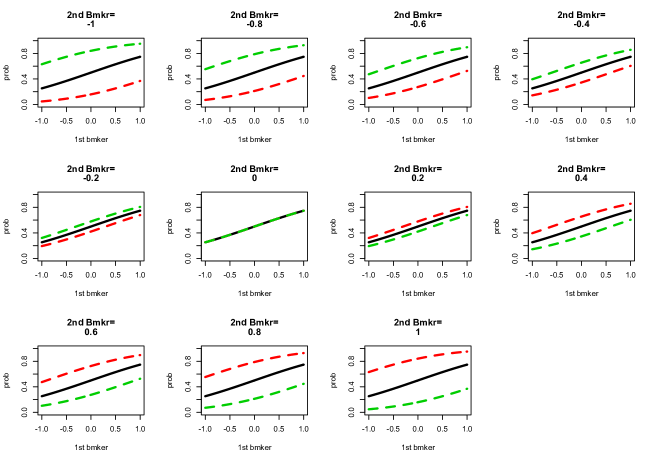
We consider six scenarios and simulated $1,000$ trials for each scenario. In the first two scenarios, we assume that biomarkers $x_{i1}$ and $x_{i2}$ are relevant to the response, but not biomarkers $x_{i3}$ and $x_{i4}$. The simulation truth for the outcome $y_{i}$ is a probit regression. Specifically, we assume that the true response rates for a patient with covariate vector $\bm{x}_{i}$ under treatments 1, 2 or 3 are $\theta_{1i}=\Phi_{\mu=0,\sigma=1.5}(x_{i1}+1.5x_{i2})$, $\theta_{2i}=\Phi_{\mu=0,\sigma=1.5}(x_{i1})$, or $\theta_{3i}=\Phi_{\mu=0,\sigma=1.5}(x_{i1}-1.5x_{i2})$, respectively, where $\Phi_{\mu=0,\sigma=1.5}$ is the cumulative distribution function (CDF) of a Gaussian distribution with $\mu=0$ and $\sigma=1.5$. Figure 2 plots the response rates under three treatments versus $x_{i1}$ given different values of $x_{i2}$. The red lines represent treatment 1, black lines refer to treatment 2 and green lines to treatment 3. Treatment 3 is always the most effective arm when $x_{i2}<0$, the three treatments have equal success rates when $x_{i2}=0$, and treatment 1 is superior when $x_{i2}>0$. In summary, the optimal treatment is a function of the second biomarker, $x_{i2}$. That is, $x_{i2}$ identifies the optimal treatment selection. The response rates of three treatments increase with $x_{i1}$, but the ordering of the three treatments does not change varying the first biomarker. Therefore, $x_{i1}$ is only predictive of response, but ideally should not be involved for treatment selection. To assess the performance of SUBA under this setup, we select two scenarios. In an over-simplified scenario 1, we assume that all the patients have $x_{i2}=0.8$. Thus, treatment 1 is more effective than 2, which in turn is more effective than 3. In scenario 2, we do not fix the values of $x_{i2}$ and randomly generate all biomarker values.

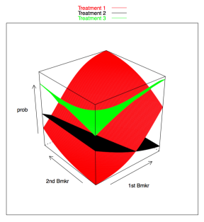
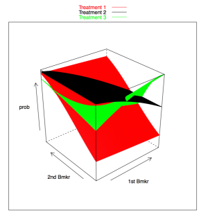
In scenario 3, we assume that biomarkers 1, 2 and 3 are related to the response and there are interactions. The true response rates under treatments 1, 2, or 3 are $\theta_{1i}=\Phi_{\mu=0,\sigma=1.5}(x_{i1}+1.5x_{i2}-0.5x_{i3}+2x_{i1}x_{i3})$, $\theta_{2i}=\Phi_{\mu=0,\sigma=1.5}(-x_{i1}-2x_{i3})$, or $\theta_{3i}=\Phi_{\mu=0,\sigma=1.5}(x_{i1}-1.5x_{i2}-2x_{i1}x_{i2})$, respectively. Figure 3 plots the response rates under three treatments versus $(x_{i1},x_{i2})$ given $x_{i3}=0.6$ (Figure 3a) and given $x_{i3}=-0.6$ (Figure 3b). Here, all three markers are predictive of the ordering of the treatment effects in a complicated fashion.

We design scenarios 4 and 5 with treatment 3 being uniformly inferior to treatments 1 and 2. We assume that the response rates under treatments 1 and 2 are $\theta_{1i}=\Phi_{\mu=0,\sigma=1.5}(x_{i1}^{2}/2+x_{i1}x_{i2}/2)$ or $\theta_{2i}=\Phi_{\mu=0,\sigma=1.5}(x_{i2}^{2}/2-x_{i1}x_{i2}/2)$. The implied minimum response rate for treatments 1 and 2 is 0.37 and the response rates of treatment 1 and 2 are close for all biomarker values (differences range from -0.24 to 0.24 with the first quantile across biomarker profiles equal to -0.06 and the third quantile equal to 0.09). We assume $\theta_{3i}=0.15$ in scenario 4 and $\theta_{3i}=0.3$ in scenario 5, thus $\theta_{3i}\leq\min(\theta_{1i},\theta_{2i})$ for all $x_{i1}$ and $x_{i2}$. So we can expect that treatment 3 should be excluded in both scenarios.

Finally, Scenario 6 is a null case, in which no biomarkers are related to response. We assume that the response rates under the three treatments for all the patients are the same at 40%, that is, $\theta_{1i}=\theta_{2i}=\theta_{3i}=0.4$.

Comparison.

For comparison, we implement a standard design with equal randomization (ER), an outcome-adaptive randomization (AR) design, and a design based on a probit regression model (Reg). In the ER design, all patients are equally randomized to the three treatments and their responses are generated from $\mathrm{Bernoulli}(\theta_{ti})$ for patient $i$ receiving treatment $t$, $t=1,2,3$ and $i=1,\dots,N$. The values of $\theta_{ti}$ are defined by the Gaussian CDFs given above. Under the AR design, we assume that three predefined biomarker subgroups are fixed before the trial (similar to the BATTLE trial Kim et al. (2011)). We assume that the three subgroups are defined as $\{x_{i1}<-0.5\}$, $\{-0.5\leq x_{i1}\leq 0.5\}$ and $\{x_{i1}>0.5\}$, using the quartiles of the empirical distribution of biomarker $x_{i1}$ as thresholds. Apparently, these subgroups are wrongly defined and do not match the true response curves in scenarios 1-6. The mismatch is deliberately chosen to evaluate the importance of correctly defining subgroups. Let $p_{tb}$ be the response rate of treatment $t$ in subgroup $b$, and $n_{tb}$ the total number of patients receiving treatment $t$ in subgroup $b$, $t=1,2,3$ and $b=1,2,3$. For this design we use the model $y_{i}\mid x_{i}\in b\sim\mathrm{Binomial}(n_{tb},p_{tb})$. With a conjugate beta prior distribution beta(1,1) on $p_{tb}$, we easily compute the posterior of $p_{tb}$ as $p_{tb}\mid\mathcal{D}\sim\mathrm{beta}(n_{tb1}+1,n_{tb}-n_{tb1}+1)$, where $n_{tb1}$ is the number of patients who responded to treatment $t$ in subgroup $b$. Then under the AR design, we first equally randomize 100 patents to the three treatments, and adaptively randomize the next 200 patents sequentially. The AR probability for a future patient in subgroup $b$ equal $\hat{p}_{tb}/(\hat{p}_{1b}+\hat{p}_{2b}+\hat{p}_{3b})$, where $\hat{p}_{tb}$ is the posterior mean $(n_{tb1}+1)/(n_{tb}+2)$, alternatively other summaries of the $(p_{1b},p_{2b},p_{3b})$ posterior can be used to adapt treatment assignment Thall and Wathen (2007). Under the Reg design, we model binary outcomes using a probit regression. In the probit model, the inverse standard normal CDF of the response rate is modeled as a linear combination of the biomarkers and treatment, $p(y_{i}=1\mid z_{i},\bm{x}_{i})=\Phi(\beta_{0}z_{i}+{\bm{\beta}}^{\prime}_{1}\bm{x}_{i})$. The parameters $\beta_{0}$ and ${\bm{\beta}}_{1}=(\beta_{11},\ldots,\beta_{1k})$ are obtained using maximum likelihood estimation. Under the Reg design, we randomize the first 100 patients with equal probabilities to the three treatments, and then assign the next 200 patients to the treatment with estimated best success probability, sequentially.

3.2 Simulation Results

Response rates.

Define the overall response rate (ORR) as

$$\mathrm{ORR}=\frac{1}{N-n}\sum_{i=n+1}^{N}I(y_{i}=1),$$

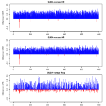
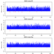
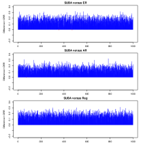
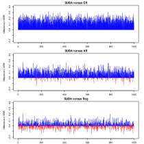
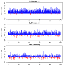
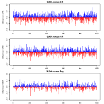
which is the proportion of responders among those patients who are treated after the run-in phase. We summarize ORR differences between SUBA versus ER, AR, and Reg for each scenario in Figure 4. In our comparisons we use the same burn in period $n=100$ across designs.

For scenarios 2 and 3, SUBA outperforms ER, AR and Reg with higher ORR in almost all the simulated trials. The ER and AR designs perform similarly. This suggests that no gains are obtained with AR when the biomarker subgroups are wrongly defined, confirming that for AR it is essential an upfront appropriate selection of the biomarker subgroups. In scenarios 1, 4 and 5, SUBA and Reg are preferable to ER and AR. SUBA exhibits a larger ORR value than Reg in 676 of 1,000 simulations in scenario 1, in 612 of 1,000 simulations in scenario 4 and in 605 of 1,000 simulations in scenario 5. In scenario 6, the true response rates are constant and not related to biomarkers, and the four designs show similar ORRs distribution across 1,000 simulations.

Early stopping.

Table 1 reports the average number of patients under the SUBA design. When a trial is stopped early by SUBA, there must be one last treatment left which are considered more efficacious than all the removed treatments. For a fair comparison with ER, AR and Reg which do not include early stopping, summaries in Table 2 are based on assignment of all remaining patients, until the maximum sample size $N$, to that last active arm.

Scenario	1	2	3	4	5	6
# of patients	245.28	299.41	300.00	167.63	215.07	209.52

Table 1: The average numbers of patients needed to make the decision of stopping trials early in 1,000 simulated trials in scenarios 1-6.

Treatment assignment.

We compute the average number of patients (ANP) assigned to treatment $t$ after the run-in phase by the three designs. Denote $\mathrm{NP}^{d}_{t}$ as the number of patients assigned to treatment $t$ in $d^{th}$ simulated trial after the run-in phase, i.e., $\mathrm{NP}^{d}_{t}=\sum_{i=n+1}^{N}I(z^{\star}_{i}=t)$, $t=1,2,3$ and $d=1,\dots,1000$. Thus

$$\mathrm{ANP}_{t}=\frac{1}{1000}\sum_{d=1}^{1000}\mathrm{NP}^{d}_{t}.$$

Table 2 shows the results. In scenario 1, treatment 1 is always the most effective arm since the second biomarker is fixed at 0.8 (see Figure 2). We can see that most of the patients are allocated to treatment 1 in scenario 1 by SUBA. Scenario 6 is a null case in which the biomarkers are not related to response rates and the response rates across treatments are the same, so the patients allocation by SUBA is similar as ER, AR and Reg.

Scenario			ER			AR			Reg			SUBA
	Subset	1	2	3	1	2	3	1	2	3	1	2	3
1	/	66.76	66.60	66.64	83.02	65.35	51.63	119.46	70.13	10.41	177.11	18.67	4.22
2	$S_{1}^{0}$	33.49	33.09	33.24	33.37	33.19	33.25	35.24	32.88	31.69	72.57	18.37	8.88
	$S_{2}^{0}$	33.27	33.51	33.40	33.41	33.25	33.53	35.42	33.01	31.76	8.63	17.79	73.77
3	$S_{1}^{0}$	19.49	19.09	19.29	22.21	17.63	18.03	18.65	16.40	22.81	41.11	8.94	7.82
	$S_{2}^{0}$	25.23	25.17	25.35	21.13	26.81	27.80	24.10	21.86	29.79	13.67	35.91	26.17
	$S_{3}^{0}$	22.05	22.34	22.00	24.61	20.52	21.26	21.27	18.99	26.12	11.33	11.54	43.52
4	$S_{1}^{0}$	33.26	33.11	33.44	43.01	42.32	14.49	51.81	48.00	0	52.76	46.96	0.10
	$S_{2}^{0}$	33.50	33.49	33.20	42.32	43.46	14.41	51.75	48.44	0	50.78	49.29	0.11
5	$S_{1}^{0}$	33.26	33.11	33.44	39.14	38.49	22.19	51.51	48.25	0.05	51.13	47.05	1.63
	$S_{2}^{0}$	33.50	33.49	33.20	38.29	39.32	22.58	51.22	48.92	0.05	47.07	51.53	1.59
6	/	66.76	66.60	66.64	66.66	66.89	66.46	65.04	67.84	67.12	66.90	64.20	68.90

Table 2: The average numbers of patients (ANPs) assigned to three treatments after the run-in phase in three defined subsets by ER, AR, Reg and SUBA in 1,000 simulated trials in scenarios 1-6.

In scenario 2, we separately report the average numbers of patients assigned to three treatments after the run-in phase, among those whose second biomarker is positive or negative. We separately report these two averages to demonstrate the benefits of using the SUBA design since depending on the sign of the second biomarker, different treatments should be selected as the most beneficial and effective ones for patients. When the second biomarker is positive, treatment 1 is the most superior arm; when the second biomarker is negative, treatment 3 is the most effective arm according to our simulation settings. From Table 2, among the 200 post-runin patients, about 100 patients have ($x_{i2}>0$) values of the second biomarker. In Table 2 we use $S^{0}_{1}=\{i:x_{i2}>0\}$ and $S^{0}_{2}=\{i:x_{i2}<0\}$ to denote sets of patients. Think of $\{S^{0}_{1},S^{0}_{2}\}$ as a partition in the simulation truth. Among patients in $S^{0}_{1}$, Table 2 reports that an average of approximately 73 of them are allocated to treatment 1, 18 to treatment 2, and 9 to treatment 3. For those in $S^{0}_{2}$, 9 are allocated to treatment 1, 18 to treatment 2, and 74 to treatment 3. Most of the patients are assigned to the correct superior treatments according to their biomarker values, highlighting the utility of the SUBA design. In contrast, ER, AR and Reg designs assign far fewer patients to the most effective treatments. These results and, similarly Figure 4, shows the utility of the SUBA approach.

In scenario 3, biomarkers 1, 2 and 3 are related to the response. In a similar fashion, we report patient allocations by breaking down the numbers according to three subsets that are indicative of the true optimal treatment allocation depending on the biomarker values. Denote $\bar{\theta}_{1i}=x_{i1}+1.5x_{i2}-0.5x_{i3}+2x_{i1}x_{i3}$, $\bar{\theta}_{2i}=-x_{i1}-2x_{i3}$, and $\bar{\theta}_{3i}=x_{i1}-1.5x_{i2}-2x_{i1}x_{i2}$. According to the simulation truth, we consider three sets $S^{0}_{1},S^{0}_{2}$ and $S^{0}_{3}$, defined as $S^{0}_{1}=\{i:\bar{\theta}_{1i}>\bar{\theta}_{2i}\ \mathrm{and}\ \bar{\theta}_{1i}>\bar{\theta}_{3i}\}$, $S^{0}_{2}=\{i:\bar{\theta}_{2i}>\bar{\theta}_{1i}\ \mathrm{and}\ \bar{\theta}_{2i}>\bar{\theta}_{3i}\}$ and $S^{0}_{3}=\{i:\bar{\theta}_{3i}>\bar{\theta}_{1i}\ \mathrm{and}\ \bar{\theta}_{3i}>\bar{\theta}_{2i}\}$. Under this assumption, the best treatment for patients in set $S^{0}_{t}$ is treatment $t$ according to the simulation truth. Table 2 reports the simulation results for $S^{0}_{1}$, $S^{0}_{2}$ and $S^{0}_{3}$. We can see most of the patients are assigned to the correct superior treatments. In contrast, the ER, AR and Reg designs fail to do so.

In scenarios 4 and 5, biomarkers 1 and 2 are related to the response. Since treatment 3 is inferior to treatments 1 and 2, the biomarker space is only split to two sets $S^{0}_{1}$ and $S^{0}_{2}$ according to simulation truth. Denote $\bar{\theta}_{1i}=x_{i1}^{2}/2+x_{i1}x_{i2}/2$, $\bar{\theta}_{2i}=x_{i2}^{2}/2-x_{i1}x_{i2}/2$. So $S^{0}_{1}=\{i:\bar{\theta}_{1i}>\bar{\theta}_{2i}\}$ and $S^{0}_{2}=\{i:\bar{\theta}_{2i}>\bar{\theta}_{1i}\}$. Table 2 again shows that SUBA assigns more patients to their corresponding optimal treatments than ER and AR designs, but performs similar as Reg. Scenarios 4-5 are two challenging cases, in which the dose-response surfaces are “U”-shaped (plots not shown) and treatments 1 and 2 have similar true responses rates for most biomarker values. Treatment 3 is much less desirable to treatments 1 and 2, and is excluded by SUBA and Reg quickly across most of the simulations. Both designs assign similar numbers of patients on average to treatments 1 and 2. However, both designs assign a considerable number of patients to suboptimal treatments. For example, in both scenarios 50% of the patients received a suboptimal treatment, which could be caused by false negative splits that failed to capture the superior subgroups for those patients. Nevertheless, SUBA is still markedly better than the ER and AR designs in these scenarios.

In summary, SUBA continuously learns the response function to pair optimal treatments with targeted patients and can substantially outperform ER, AR and Reg in terms of OOR.

Posterior estimated partition.

Figure 6 shows the least-square partition $\Pi^{LS}$ in an arbitrarily selected trial for scenarios 2 and 3. The number in each circle represents the biomarker used to split the biomarker space. In scenario 2, biomarkers 1 and 2 are related to response rate. Treatment 1 is the best treatment when the second biomarker is positive and treatment 3 is the best one when the second biomarker is negative. The least-square partition $\Pi^{LS}$ uses biomarker 2 to split the biomarker space in the first round of split, which corresponds to the simulation truth. In scenario 3, biomarkers 1, 2, and 3 are related to response rate and the least-square partition $\Pi^{LS}$ uses these true response-related biomarkers to split as well.

3.3 Sensitivity Analysis

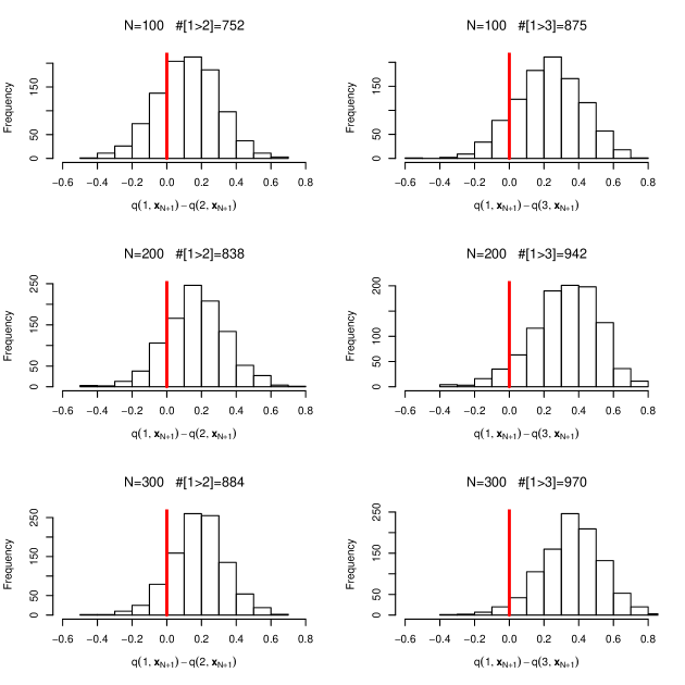
To evaluate the impact of the maximum sample size on the simulation results, we carried out a sensitivity analysis with $N=100,200,300$ in scenario 1, with first $n=100$ patients equally randomized. Recall that in scenario 1, treatment 1 has a higher response rate than treatments 2 and 3, regardless of their biomarker values. Therefore the effect of sample size on the posterior inference can be easily evaluated.

Figure 5 plots the histogram of differences between treatments $q_{N+1}(1,\bm{x}_{n+1})-q_{N+1}(2,\bm{x}_{n+1})$ and $q_{N+1}(1,\bm{x}_{n+1})-q_{N+1}(3,\bm{x}_{n+1})$ after $N=100,200,$ or $300$ patients have been treated in the trial. When $N=100$, treatment 1 is reported as better than treatment 2 in 752 of 1,000 simulations; when $N=200$, treatment 1 is better than treatment 2 in 838 of 1,000 simulations; when $N=300$, treatment 1 is better than treatment 2 in 884 of 1,000 simulations. The more patients treated, the more precise the posterior estimates and more accurate assignments for future patients. Similar patterns are observed for the comparison between treatments 1 and 3.

We also varied the values $\phi$ and conducted sensitivity analysis with $\phi=0.2,0.5,0.8$ using scenario 2. Table 3 shows the average numbers of patients needed to make the decision of stopping trials early and the average numbers of patients assigned to three treatments after the run-in phase in two defined subsets. In summary, the reported summaries vary little across the considered hyperparameter choices, indicating robustness with respect to changes within a reasonable range of values.

		$\phi=0.2$			$\phi=0.5$			$\phi=0.8$
# of patients		298.10			299.41			299.15
Subset	1	2	3	1	2	3	1	2	3
$S^{0}_{1}$	71.66	19.09	9.06	72.57	18.37	8.88	72.21	18.50	9.11
$S^{0}_{2}$	8.64	18.50	73.05	8.63	17.79	73.77	8.79	18.31	73.09

Table 3: The average numbers of patients needed to make the decision of stopping trials early and patient allocation breakdowns in scenario 2 with different values of $\phi=0.2,0.5,0.8$.

4 Discussion

We demonstrated the importance of subgroup identification in adaptive designs when such subgroups are predictive of treatment responce. The key contribution of the proposed model-based approach is the construction of the random partition prior $p(\Pi)$ which allows a flexible and simple mechanism to realize subgroup exploration as posterior inference on $\Pi$. The Bayesian paradigm facilitates continuous updating of this posterior inference as data becomes available in the trial. The proposed construction for $p(\Pi)$ is easy to interpret and, most importantly, achieve a good balance between the required computational burden for posterior computation and the flexibility of the resulting prior distribution. The priors of $\theta_{t,m}$ are i.i.d Beta$(a,b)$, with $a=b=1$, i.e., a uniform prior in our simulation studies. If desired, this prior can be calibrated to reflect the historical response rate of the drug. The i.i.d assumption simplifies posterior inference. Alternatively, one could impose dependence across the $\theta$’s; for example, one could assume that adjacent partition sets have similar $\theta$ values.

The proposed SUBA design focuses on the treatment success for the patients who are enrolled in the current trial by identifying subgroups of patients who respond most favorably to each of the treatments. One could easily add to the SUBA algorithm a final recommendation of a suitable patient population for a follow-up trial, such as $\Pi^{LS}$. Other directions of generalization include an extension of the models to incorporate variable selection, when a large number of biomarkers are measured.

Figure 1: An illustration of $p(\Pi)$ with three rounds splits. The example shows that with three rounds of split, the initial space of two biomarkers is partitioned into five sets $\{UU_{11},UL_{11},LL_{12},LUU_{121},LUL_{121}\}$.

Figure 2: Display of Scenario 2. The probabilities of response versus the measurements of the first biomarker given fixed values of the second biomarker. Red, black and green lines represent three treatments 1, 2 and 3 respectively.

(a) When 3rd biomarker=0.6	(b) When 3rd biomarker=-0.6

Figure 3: Display of Scenario 3. The probabilities of response versus the measurements of the first and the second biomarkers given the fixed values of the third biomarker at 0.6 (a) and -0.6 (b). Red, black and green lines represent three treatments 1, 2 and 3 respectively.

Scenario 1	Scenario 2	Scenario 3
Scenario 4	Scenario 5	Scenario 6

Figure 4: The overall response rate (ORR) comparisons among the ER, AR, Reg and SUBA designs in 1,000 simulated trials in all six scenarios. We plot the ORR differences between SUBA and ER, AR, Reg respectively in each scenario. The blue color represents the ORR of SUBA is higher than ER, AR or Reg; the red color represents lower.

Figure 5: The histogram of $q_{N+1}(1)-q_{N+1}(2)$ and $q_{N+1}(1)-q_{N+1}(3)$ when $N=100,200,300$. The right side of red vertical line indicates that the posterior predictive rate of treatment 1 is higher than treatment 2 or treatment 3.

(a) Scenario 2

(b) Scenario 3

Figure 6: The tree-type least-square partition by SUBA design in one simulated trial in scenarios 2 and 3. The number in the circle represents the biomarker used to split the biomarker space.

References

- Baladandayuthapani et al. (2010) Baladandayuthapani, V., Y. Ji, R. Talluri, L. E. Nieto-Barajas, and J. S. Morris (2010). Bayesian random segmentation models to identify shared copy number aberrations for array cgh data. Journal of the American Statistical Association 105(492).
- Barker et al. (2009) Barker, A., C. Sigman, G. Kelloff, N. Hylton, D. Berry, and L. Esserman (2009). I-spy 2: an adaptive breast cancer trial design in the setting of neoadjuvant chemotherapy. Clinical Pharmacology & Therapeutics 86(1), 97–100.
- Barski and Zhao (2009) Barski, A. and K. Zhao (2009). Genomic location analysis by chip-seq. Journal of cellular biochemistry 107(1), 11–18.
- Chipman et al. (1998) Chipman, H. A., E. I. George, and R. E. McCulloch (1998). Bayesian cart model search. Journal of the American Statistical Association 93(443), 935–948.
- Curtis et al. (2012) Curtis, C., S. P. Shah, S.-F. Chin, G. Turashvili, O. M. Rueda, M. J. Dunning, D. Speed, A. G. Lynch, S. Samarajiwa, Y. Yuan, et al. (2012). The genomic and transcriptomic architecture of 2,000 breast tumours reveals novel subgroups. Nature 486(7403), 346–352.
- Dahl (2006) Dahl, D. (2006). Model-based clustering for expression data via a dirichlet process mixture model. Bayesian inference for gene expression and proteomics, 201–218.
- Denison et al. (1998) Denison, D. G., B. K. Mallick, and A. F. Smith (1998). A bayesian cart algorithm. Biometrika 85(2), 363–377.
- Fedorov and Leonov (2013) Fedorov, V. V. and S. L. Leonov (2013). Optimal design for nonlinear response models. CRC Press.
- Foster et al. (2011) Foster, J. C., J. M. Taylor, and S. J. Ruberg (2011). Subgroup identification from randomized clinical trial data. Statistics in medicine 30(24), 2867–2880.
- Freidlin et al. (2010) Freidlin, B., L. M. McShane, and E. L. Korn (2010). Randomized clinical trials with biomarkers: design issues. Journal of the National Cancer Institute 102(3), 152–160.
- Gelfand and Ghosh (1998) Gelfand, A. E. and S. K. Ghosh (1998). Model choice: A minimum posterior predictive loss approach. Biometrika 85(1), 1–11.
- Gu and Lee (2010) Gu, X. and J. J. Lee (2010). A simulation study for comparing testing statistics in response-adaptive randomization. BMC medical research methodology 10(1), 48.
- Hudis (2007) Hudis, C. A. (2007). Trastuzumab?mechanism of action and use in clinical practice. New England Journal of Medicine 357(1), 39–51.
- Kim et al. (2011) Kim, E. S., R. S. Herbst, I. I. Wistuba, J. J. Lee, G. R. Blumenschein, A. Tsao, D. J. Stewart, M. E. Hicks, J. Erasmus, S. Gupta, et al. (2011). The battle trial: personalizing therapy for lung cancer. Cancer Discovery 1(1), 44–53.
- Kruschke (2008) Kruschke, J. (2008). Bayesian approaches to associative learning: from passive to active learning. Learning & Behavior 36, 210–226.
- Loredo (2003) Loredo, T. (2003). Bayesian adaptive exploration in a nutshell. Statistical Problems in Particle Physics, Astrophysics, and Cosmology 1, 162–165.
- Maitournam and Simon (2005) Maitournam, A. and R. Simon (2005). On the efficiency of targeted clinical trials. Statistics in medicine 24(3), 329–339.
- Mandrekar and Sargent (2010) Mandrekar, S. J. and D. J. Sargent (2010). Predictive biomarker validation in practice: lessons from real trials. Clinical Trials 7(5), 567–573.
- Medvedovic et al. (2004) Medvedovic, M., K. Y. Yeung, and R. E. Bumgarner (2004). Bayesian mixture model based clustering of replicated microarray data. Bioinformatics 20(8), 1222–1232.
- Misale et al. (2012) Misale, S., R. Yaeger, S. Hobor, E. Scala, M. Janakiraman, D. Liska, E. Valtorta, R. Schiavo, M. Buscarino, G. Siravegna, et al. (2012). Emergence of kras mutations and acquired resistance to anti-egfr therapy in colorectal cancer. Nature 486(7404), 532–536.
- Mitra et al. (2013) Mitra, R., P. Müller, S. Liang, L. Yue, and Y. Ji (2013). A bayesian graphical model for chip-seq data on histone modifications. Journal of the American Statistical Association 108(501), 69–80.
- Raiffa and Schlaifer (1961) Raiffa, H. and R. Schlaifer (1961). Applied statistical decision theory (harvard business school publications).
- Ruberg et al. (2010) Ruberg, S. J., L. Chen, and Y. Wang (2010). The mean does not mean as much anymore: finding sub-groups for tailored therapeutics. Clinical Trials 7(5), 574–583.
- Sargent et al. (2005) Sargent, D. J., B. A. Conley, C. Allegra, and L. Collette (2005). Clinical trial designs for predictive marker validation in cancer treatment trials. Journal of Clinical Oncology 23(9), 2020–2027.
- Simon (2010) Simon, R. (2010). Clinical trial designs for evaluating the medical utility of prognostic and predictive biomarkers in oncology. Personalized medicine 7(1), 33–47.
- Simon and Maitournam (2004) Simon, R. and A. Maitournam (2004). Evaluating the efficiency of targeted designs for randomized clinical trials. Clinical Cancer Research 10(20), 6759–6763.
- Snijders et al. (2001) Snijders, A. M., N. Nowak, R. Segraves, S. Blackwood, N. Brown, J. Conroy, G. Hamilton, A. K. Hindle, B. Huey, K. Kimura, et al. (2001). Assembly of microarrays for genome-wide measurement of dna copy number. Nature genetics 29(3), 263–264.
- Thall and Wathen (2007) Thall, P. F. and J. K. Wathen (2007). Practical bayesian adaptive randomisation in clinical trials. European Journal of Cancer 43(5), 859–866.
- Van De Vijver et al. (2002) Van De Vijver, M. J., Y. D. He, L. J. van’t Veer, H. Dai, A. A. Hart, D. W. Voskuil, G. J. Schreiber, J. L. Peterse, C. Roberts, M. J. Marton, et al. (2002). A gene-expression signature as a predictor of survival in breast cancer. New England Journal of Medicine 347(25), 1999–2009.
- Wang et al. (2008) Wang, Z., C. Zang, J. A. Rosenfeld, D. E. Schones, A. Barski, S. Cuddapah, K. Cui, T.-Y. Roh, W. Peng, M. Q. Zhang, et al. (2008). Combinatorial patterns of histone acetylations and methylations in the human genome. Nature genetics 40(7), 897–903.
- Yin et al. (2012) Yin, G., N. Chen, and J. Jack Lee (2012). Phase ii trial design with bayesian adaptive randomization and predictive probability. Journal of the Royal Statistical Society: Series C (Applied Statistics) 61(2), 219–235.
- Zhu et al. (2013) Zhu, H., F. Hu, and H. Zhao (2013). Adaptive clinical trial designs to detect interaction between treatment and a dichotomous biomarker. Canadian Journal of Statistics, 1–15.