22email: kabir.ramola@u-psud.fr 33institutetext: C. Texier 44institutetext: Univ. Paris Sud ; CNRS ; Laboratoire de Physique Théorique et Modèles Statistiques, UMR 8626 ; 91405 Orsay cedex, France
44email: christophe.texier@u-psud.fr
Fluctuations of random matrix products and 1D Dirac equation with random mass
Abstract
We study the fluctuations of certain random matrix products of , describing localisation properties of the one-dimensional Dirac equation with random mass. In the continuum limit, i.e. when matrices ’s are close to the identity matrix, we obtain convenient integral representations for the variance . The case studied exhibits a saturation of the variance at low energy along with a vanishing Lyapunov exponent , leading to the behaviour as . Our continuum description sheds new light on the Kappus-Wegner (band center) anomaly.
PACS numbers : 72.15.Rn ; 02.50.-r
1 Introduction
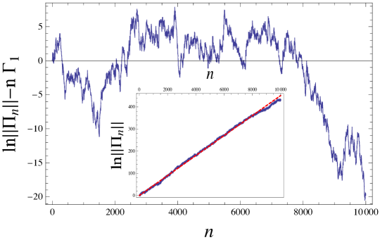
Transfer matrices lead to a convenient formulation of many statistical physics problems and have been extensively used since their introduction in the context of the Ising model Bax82 . In the presence of randomness, most of the physics is captured by the Lyapunov exponent which quantifies the growth rate of the matrix elements of a random matrix product (RMP) . Given the measure characterizing the independent and identically distributed random matrices ’s, the Furstenberg formula allows one to obtain, at least in principle, the Lyapunov exponent , where is a suitable norm, in terms of the solution of the Furstenberg’s integral equation BouLac85 . Besides the Lyapunov exponent, which describes the mean free energy of the random Ising model Luc92 ; CriPalVul93 ; FigMosKno98 , the fluctuations of RMP (Fig. 1) also play an important role and are the main subject of this paper.
The study of fluctuations is related to the generalised Lyapunov exponent analysis Luc92 ; CriPalVul93 111Generalised central limit theorems for matrices was discussed in the mathematical literature (chapter V of the monograph BouLac85 ). and the multifractal formalism introduced by Paladin and Vulpiani PalVul87b ; PalVul87 . Fluctuations are of particular importance in the context of quantum localisation, where they dominate several physical quantities, like the local density of states AltPri89 or the Wigner time delay TexCom99 . Their precise characterisation is an important issue at the heart of the scaling approach used in the justification of the single parameter scaling (SPS) hypothesis (cf. Refs. AndThoAbrFis80 ; CohRotSha88 and references therein). In the last decade, this question has been re-examined more precisely for a lattice model DeyLisAlt00 ; SchTit03 ; TitSch05 . Recently Lyapunov exponents have been analytically obtained for general RMPs of in the continuum limit ComLucTexTou13 . This has significantly improved our understanding of RMPs and of one-dimensional (1D) quantum localisation models due to their close connection ComTexTou10 . The present work is a first step towards generalising this approach for the fluctuations. We will consider matrices belonging to two particular subgroups of :
| (1) |
or
| (2) |
We will show in section 2 that products of matrices of the type (1) are transfer matrices for the bi-spinor solution of the 1D Dirac equation
| (3) |
for a mass of the form and with , where ’s are Pauli matrices. Matrices of the type (2) with correspond to the case . The Dirac equation (3) with random mass is a relevant model in several contexts of condensed matter, e.g. random spin chains or organic conductors (see references in Refs. LeDMonFis99 ; TexHag10 ). It can also be exactly mapped onto supersymmetric quantum mechanics ComTex98 and the Sinai problem of 1D classical diffusion in a random force field BouComGeoLeD90 ; LeDMonFis99 . Many properties of the model can be obtained exactly when the mass is chosen to be a Gaussian white noise :
| (4) |
where . For example the Lyapunov exponent, defined in the localisation problem as , is known BouComGeoLeD90
| (5) |
where is the Hankel function. The case is of particular interest since the Lyapunov exponent vanishes as , indicating a delocalisation point in the spectrum. In this unusual case, the characterisation of (i.e. ) is thus crucial. We will show that the fluctuations saturate as , and thus dominate localisation properties.
2 Mapping
The mapping between RMP and 1D localisation models like the random Kronig-Penney model Luc92 , was recently extended to general RMPs of ComTexTou10 . For the case of interest here, the mapping works as follows : consider a random mass given as a superposition of delta-functions , where coordinates are ordered . Matching conditions across each impurity read and , hence the diagonal matrix in (1), while the rotation of angle stands for the free evolution between two impurities. If we consider the Dirac equation with a purely imaginary energy , the matrix (2) with , relates at and . 222Note that matrices (2) with and are tranfer matrices for the random Ising chain with couplings and magnetic fields Luc92 ; a continuum approximation of the model was considered in Ref. FigMosKno98 allowing these authors to recover the Lyapunov exponent (5) obtained first in Ref. BouComGeoLeD90 . The product thus controls the value of the spinor and the study of the growth of the RMP characterizes the localisation properties of the wave function. It is convenient to introduce the Riccati variable ; from Eq. (3), we find
| (6) |
If the lengths are either equal (lattice) or distributed with an exponential law , the stochastic differential equation (SDE) defines a Markov process. Hence, shows that and are asymptotically equivalent, thus their cumulants are related by . In the following we will consider the continuum limit of the RMP problem when the random parameters are small and , i.e. the matrices are close to the identity matrix, in such a way that and is fixed ; this limit corresponds to the case where is a Gaussian white noise with zero mean ComLucTexTou13 ; ComTexTou13 . The SDE (6) must be interpreted in the Stratonovich convention as is usual in physical problems Gar89 . The study of the fluctuations of the RMP can be performed by introducing the generalised Lyapunov exponent PalVul87 ; CriPalVul93
| (7) |
which is the generating function for the cumulants of . In the following discussion we focus on . From the definition of the Riccati variable, we may write , hence
| (8) |
It is convenient to use the relation
| (9) |
obtained by integration of (6). Finally we get
| (10) |
The propagator is defined as
| (11) |
where is the conditional probability, solution of the Fokker-Planck equation , and is the stationary distribution of the Riccati variable, with
| (12) |
being the forward generator of the diffusion (adjoint of the generator). Eq. (10) is one of our main results : can be explicitly obtained as the normalisable solution of and solves
| (13) |
Note that, in the derivation of the second term of (10), we have used the underlying supersymmetry of the Dirac equation ComTexTou10 ; ComTexTou13 , leading to . Solving the equation for , we can obtain an explicit representation for in terms of multiple integrals, like it is done for another subgroup of in Appendix C. We prefer to proceed in a different manner in order to derive limiting values for .
3 Universal regime (large real energy )
The large energy limit is the universal regime where SPS holds CohRotSha88 : a unique scale controls the average and the fluctuations . The variance was explicitly calculated for this model in Ref. Tex99 and coincides with the known value for the Lyapunov exponent BouComGeoLeD90 , Eq. (5), that saturates at high energy : (Fig. 2).
4 Small real energy
The process flows through the full interval and it is convenient to consider the variable
| (14) |
When goes from to the process crosses once, and a second time when goes from to . The new process obeys the SDE
| (15) |
for the unbounded potential
| (16) |
Rewriting (10) in terms of the new variable, we get
| (17) |
where and
| (18) |
for the forward generator
| (19) |
The details of the derivation of Eq. (17) are given in Appendix A. The variable is appropriate for the low energy analysis : the exponential dependence of the potential clearly illustrates the decoupling between the “deterministic force” and Langevin “force” . We can map the problem onto an effective free diffusion problem in the interval , where . The form of at infinity leads to the boundary conditions : absorption at one boundary, , with reinjection of the current at the other boundary, . The stationary distribution takes the approximate form
| (20) |
and the solution of Eq. (18) is given by
| (21) |
where is the Heaviside function, and . As a check, we recover that the Lyapunov exponent
| (22) |
vanishes as
| (23) |
a behaviour which coincides with the asymptotic of the exact result (5). We easily compute (17), leading to
| (24) |
which shows the saturation of the fluctuations as .
5 Small complex energy
For complex energy , the process is trapped on . The SDE (15) still holds for the bounded potential
| (25) |
Making use of the fact that is symmetric, we can show that the representations (17) and (22) are still valid (see Appendix A), the stationary distribution being now an equilibrium distribution . In the low energy limit, we again use the decoupling between the deterministic force and the Langevin force : the effect of the confining potential is now replaced by reflecting boundary conditions . The stationary distribution is
| (26) |
thus (22) again leads to (23). The propagator takes the form
| (27) |
and Eq. (17) gives
| (28) |
This shows that, as a function of , the variance is continuous around . Setting , a more direct analysis can be performed (Appendix B) showing that
| (29) |
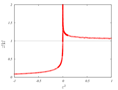
The small discrepancy () is explained by the fact that the constant term in (24,28) is sensitive to the precise position of the cutoffs of the free diffusion approximation. Numerical calculations confirm the saturation and suggest a logarithmic behaviour, although it is difficult to precisely fit this logarithmic correction (Fig. 2).

6 Large complex energy : A perturbative treatment of the stochastic differential equation
In this case, it is convenient to develop a perturbative approach based on the SDE (6). We perform the rescaling
| (30) |
leading to
| (31) |
where is a normalised Gaussian white noise, . The perturbative parameter is . Expansion of the process in powers of , as , leads to the explicit integral representations
| (32) | ||||
| (33) | ||||
| (34) |
where transient terms have been neglected. Order zero is the Ornstein-Uhlenbeck process. These expressions are suitable for computing and the correlator (8). The latter can be rewritten in terms of the rescaled process as
| (35) |
where . It is easy to see that the first non-zero contribution to this expression comes at order . We then have the following expression for to lowest order in
| (36) |
It is possible to compute this expression exactly. Since the process is derived from a Gaussian white noise source, we can use Wick’s theorem to reduce all the correlation functions to products over two-point correlation functions. However, the full calculation is rather cumbersome. Instead, we use the stochastic calculus functionalities of Mathematica 9.0 to derive the values of the correlators. We have
| (37) | ||||
| (38) | ||||
| (39) |
Summing these three contributions, we arrive at
| (40) |
7 Numerical calculations
7.1 Method
We have performed a Monte Carlo simulation of the matrix problem, i.e. of the Dirac equation for the random mass
| (41) |
where the impurities are independently and uniformly dropped on the line with a mean density . This corresponds to an exponential distribution for the distance between consecutive impurities. The mass is uncorrelated in space, i.e. is a non-Gaussian white noise. The limit of the Gaussian white noise considered in the previous sections corresponds to and with and fixed. This is a continuum model that is easy to implement numerically.
Real energy.–
We parametrize the spinor as and study the evolution of the two variables. Between impurities and we have obviously and , where we have introduced the notation and . Across the impurity BieTex08
| (42) | ||||
| (43) |
The norm of the RMP is identified with the norm of the spinor
| (44) |
Complex energy.–
For , we write the spinor as . Evolution of the two variables due to the rotation of complex angle is Tex99
| (45) | ||||
| (46) |
Evolution across an impurity are similar to the case of real energy.
7.2 The saturation of for when is a non-Gaussian white noise
For large but finite density we show that the fluctuations saturate for large complex energy . Expansion of the previous equations in the limit gives . We deduce the following representation for the process
| (47) |
where is the number of impurities on the interval . is a Poisson process and a compound Poisson process (see for instance the introduction of Ref. GraTexTou14 and references therein). Using standard properties of compound Poisson processes, we obtain
| (48) | ||||
| (49) |
(note that the cumulants of involves the moments of the jump amplitudes). Hence for with we obtain and .
7.3 Results
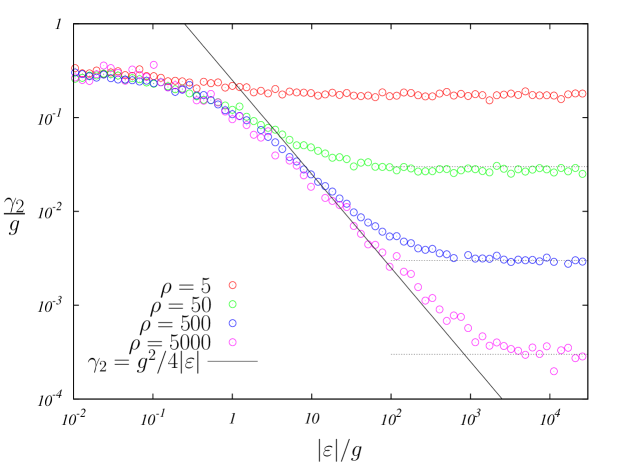
As a first check, we compare the Lyapunov exponent obtained from the procedure explained above with the analytical expression (5) : green dots and black continuous line on Fig. 2, respectively. The agreement is excellent.
For large real energy we see on the figure that saturates at the same value as (SPS). For small energy, , the inset of Fig. 2 shows the logarithmic behaviours.
The behaviour (40) is more difficult to observe as it is a property of the Dirac equation when the mass is a Gaussian white noise. The numerical simulation is performed for a non-Gaussian white noise, Eq. (41), which leads to a saturation of the fluctuations, as explained in paragraph 7.2. For this reason, the power law decay (40) is only obtained in an intermediate range of energy (Fig. 3), and we observe the saturation for . Choosing weights distributed according to a symmetric exponential law like in Ref. ComTexTou13 , the saturation value is , in agreement with the numerics (black dotted lines in Fig. 3).
8 Localisation
8.1 Low energy localisation
The saturation of the fluctuations concomitant with the vanishing of the Lyapunov exponent has important consequences for the localisation. While the Lyapunov exponent is usually introduced as a measure of the localisation (see the monographs LifGrePas88 ; Luc92 or the review ComTexTou13 ), for a given small energy , the fluctuations dominate
i.e. on a scale much larger than the inverse Lyapunov exponent . The scale has appeared in other studies : in the average Green’s function BouComGeoLeD90 (see discussion and references in Ref. SteCheFabGog99 ), in the distribution of the distances between consecutive nodes of the wave function TexHag10 , or in the boundary sensitive average local SteFabGog98 and global density of states TexHag10 (Thouless criterion). This is a new indication that the Lyapunov exponent cannot be interpreted as the inverse localisation length in this case TexHag10 ; ComTexTou13 .
8.2 Band center anomaly
The standard weak disorder expansion for the tight-binding (Anderson) model
| (50) |
is known to break down at the band center () CzyKraMac81 ; KapWeg81 . Whereas the standard expansion gives DerGar84 ; Luc92 at for uncorrelated potentials (a is the lattice spacing), the correct behaviour in the band center is DerGar84 . This small difference, vs , and those of other physical quantities, have been referred to as band center “anomalies” 333 As shown in Ref. DerGar84 , the occurence of anomalies is not specific to the band center but is an effect of commensurability. . This phenomenon may be easily analysed within our continuum description : the continuum limit of the Anderson model (50) near the band center () is the random Dirac equation Gog82
| (51) |
(for ), where and describe forward and backward (umklapp) scattering, respectively. This makes it clear that the disorder cannot be treated perturbatively for . After a rotation
| (52) |
and choosing and , this disordered model can be described by transfer matrices (1), by setting the angles . For , the Lyapunov exponent in the continuum limit is expressed in terms of elliptic integrals (this case was considered in section 6 of Ref. ComLucTexTou13 ) :
| (53) |
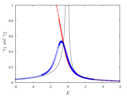
where and . For uncorrelated site potentials, , we have ; Eq. (53) with leads to , in perfect correspondence with the result of Ref. DerGar84 . at the band center was found in Ref. SchTit03 where it was shown that the anomaly is small, . On the other hand, the suppression of forward scattering 444 In the Anderson model, forward and backward scattering may be adjusted as follows : one considers random potentials , where and are two independent random functions varying smoothly at the scale of the lattice spacing . Forward scattering is controlled by the strength of whereas backward scattering is due to anti-correlation of nearest neighbour potentials, described by with strength . () leads to the model studied in the present paper with a strong anomaly at and for , Fig. 4 (the value of for finite is deduced from a continuity assumption). Our continuous description thus makes clear how one can tune the band center anomaly by adjusting the relative magnitude of forward and backward scattering.
9 Conclusion
In this paper we have characterized the statistical properties of random matrix products for two subgroups of , by making use of the fact that, for a certain choice of the distribution of the angles in (1) and (2), can be simply expressed in terms of a Markov process ComLucTexTou13 . We have deduced the variance explicitly ; the integral representations Eqs. (10,17) were demonstrated to be convenient for extracting limiting behaviours. Following Ref. PalVul87 and making use of (9), the generalised Lyapunov exponent (7) may be obtained as the largest eigenvalue of the operator . The cumulants can be obtained by using the perturbative method used in Refs. SchTit02 ; SchTit03 , however, apart from , this leads to integral representations that seem less convenient to handle. We have also obtained an integral representation similar to (10) in the case of two other particular subgroups of (see Appendix C), corresponding to the model studied in Ref. SchTit02 . It remains a challenging issue to obtain a resolution of this problem, in the spirit of the general classification of Lyapunov exponents provided recently in Ref. ComLucTexTou13 .
Acknowledgements
We acknowledge stimulating discussions with Alain Comtet, Bernard Derrida, Thierry Jolicoeur and Satya Majumdar, and a helpful suggestion of Anupam Kundu.
Appendix A Details of the derivation of Eq. (17)
A.1
For real energy, we see from the SDE (6) that the process flows towards . We have introduced the change of variable for , implying that the new process crosses twice when does once. Hence the change of variable maps the SDE (6) onto the couple of SDEs
| (54) |
In the main text we used and the local nature of the mass correlation to disregard the sign. Here we consider for the moment the general case and introduce a couple of potentials related to the cases and , respectively. is a normalised Gaussian white noise with zero mean. The process is characterised by two stationary distributions , each normalized, related to for . For example, the Lyapunov exponent is given by ComTexTou10
| (55) |
Now considering the case for which , leads to , i.e.
| (56) |
Fluctuations may be discussed in a similar way. A crucial observation is that, in the original SDE (6), the diffusion effectively vanishes at , implying the absence of correlations between the process at coordinates and associated to and . It follows that the contributions of the fluctuations related to the two intervals and simply add. The second term of (10) takes the form
For we have leading to Eq. (17).
A.2
For imaginary energy the analysis is slightly different : the process is trapped on and does not flow across . The change of variable is simply . The new process is trapped by the potential well . The equilibrium distribution is . When the potential is symmetric. We can symmetrize the expression , leading to , i.e. again to (56). Eq. (10) leads to
| (57) |
The second term can be obviously symmetrized, which gives the second term of (17). Symmetrization of the third integral term works as follows : the propagator may be decomposed over the left/right eigenvectors of the forward generator as
| (58) |
where and . Because the potential is symmetric, the eigenvectors have a symmetry property . Integration over in (57) selects only the contributions of even eigenvectors which allows one to symmetrize the integrand with respect to , leading to Eq. (17).
Appendix B Direct calculation of for
The study of the case shows some subtlety related to the choice of the norm of the matrix. In the usual case, the statistical properties of the RMP are independent of the precise definition of the norm BouLac85 ; CriPalVul93 . Bougerol and other authors propose
| (59) |
where is the norm on the vector space.
In the numerical calculation, we have parametrized the spinor as , in the spirit of the phase formalism LifGrePas88 , and study the statistical properties of , usually setting . Let us discuss the general case where may differ from . Since , the numerical procedure corresponds to considering the norm
| (60) |
i.e. . We also introduce another possible definition of the norm
| (61) |
closer to the spirit of (59).
For , the matrix product can be studied rather directly : the angles vanish and the matrices commute. Hence we can write
| (62) |
The distribution of the random variable is given by the central limit theorem : and (we consider that is fixed and fluctuates with ). We have
| (63) |
We examine first the particular case , leading to . We immediatly deduce that and , which would lead to and, incorrectly, to . The choice leads to a similar conclusion. This reflects the statistical properties of the two particular zero energy solutions
| (64) |
selected by the choices and , respectively.
We now consider the case of an arbitrary initial vector, with . In the limit, the large behaviour of the norm is selected : . Some algebra gives, for ,
| (65) |
and
| (66) |
Note that the average value is reminiscent of the average of the logarithm of the transmission probability SteCheFabGog99 (this calculation was first performed in Ref. ComMonYor98 in another context). Interestingly, the behaviours (65,66) were shown to persist in a quasi-one-dimensional situation with an odd number of channels (see the review BroMudFur01 and references therein). We obtain
| (67) | ||||
| (68) |
We can easily repeat this calculation with the second norm. Averaging of (63) over the angle gives
| (69) |
where is the elliptic integral gragra . We deduce the asymptotic behaviours for and for , leading again to (67,68).
In conclusion : for , the calculation of the cumulants is insensitive to the precise definition of the norm, i.e. to the precise choice of the initial spinor. In the Monte Carlo simulation, we have chosen in order to set a Dirichlet boundary condition for the first component of the spinor. On the other hand, setting , the behaviour of as a function of presents two discontinuities precisely at and . We understand these singular values as resulting from a lack of ergodicity in the matrix space when considering the Abelian subgroup describing the case . Hence, the value found for or should not be taken as the correct result.
Appendix C Two other subgroups of random matrices of
It is well-known that the random Kronig-Penney model for energy is controlled by transfer matrices of the form
| (70) |
where and . The Schrödinger equation with negative energy involves matrices of the form ComTexTou10
| (71) |
with the same definitions for and .
The study of the continuum limit, and with and fixed can be done along the same lines as in the paper. In this more simple case, the Riccati variable obeys the SDE . In the continuum limit is a Gaussian white noise of variance and the process is characterised by the (backward) generator . We arrive at
| (72) |
where
| (73) |
is the stationary distribution, involving the potential and the integrated density of states , given in Ref. Hal65 for instance (also recalled in Ref. GraTexTou14 ). The equation
| (74) |
for the propagator can be solved :
| (75) |
where
| (76) |
We can analyse the limiting behaviours of the variance (72). In the high energy regime, we obtain the expansions
| (77) |
(recall that ) and
| (78) | ||||
where
| (79) |
When introducing these expressions in (72), the term seems at first sight logarithmically divergent but is eliminated by symmetry (i.e. integrals must be understood as principal parts). We get
| (80) |
i.e. we have recovered the asymptotic relation for (SPS).
For , the fluctuations are finite where is a dimensionless constant of order unity (calculated explicitly in Ref. SchTit02 ). is maximum for a negative value of the energy, however the numerics shows that the ratio reaches its maximum at (Fig. 5).
The limit is more easy to handle. In this case the potential develops a deep well at , where the process is most of the “time” trapped. This dominates the fluctuations, which are those of the Ornstein-Uhlenbeck process,
| (81) |
The fluctuations thus decay faster as energy decreases than in the Dirac case studied in the paper, since the relation between the two models involves the mapping . Recalling that in this case shows that (no SPS).
Monte Carlo simulations are in perfect agreement with these behaviours (see Fig. 5).

The problem considered in this appendix was studied earlier in Refs. SchTit02 ; ZilPik03 in another context and with a different method : the generalised Lyapunov exponent (7) is obtained as the largest eigenvalue of the operator PalVul87 . The perturbative treatment SchTit02 gives an integral representation
| (82) |
where
| (83) |
Although it is not straightforward to prove the equivalence between (72) and (82), they seem to give similar results (see Fig. 1 of Ref. SchTit02 ).
References
- (1) R. J. Baxter, Exactly Solved Models in Statistical Mechanics, Academic Press, London, 1982.
- (2) P. Bougerol and J. Lacroix, Products of Random Matrices with Applications to Schrödinger Operators, Birkhaüser, Basel, 1985.
- (3) J.-M. Luck, Systèmes désordonnés unidimensionnels, CEA, collection Aléa Saclay, Saclay, 1992.
- (4) A. Crisanti, G. Paladin, and A. Vulpiani, Products of random matrices in statistical physics, Springer-Verlag, 1993, Springer Series in Solid-State Sciences vol. 104.
- (5) M. T. Figge, M. V. Mostovoy, and J. Knoester, Critical temperature and density of spin flips in the anisotropic random-field Ising model, Phys. Rev. B 58, 2626–2634 (1998).
- (6) G. Paladin and A. Vulpiani, Anomalous scaling and generalized Lyapunov exponents of the one-dimensional Anderson model, Phys. Rev. B 35, 2015–2020 (1987).
- (7) G. Paladin and A. Vulpiani, Anomalous scaling in multifractal objects, Phys. Rep. 156(4), 147–225 (1987).
- (8) B. L. Altshuler and V. N. Prigodin, Distribution of local density of states and NMR line shape in a one-dimensional disordered conductor, Sov. Phys. JETP 68(1), 198–209 (1989).
- (9) C. Texier and A. Comtet, Universality of the Wigner time delay distribution for one-dimensional random potentials, Phys. Rev. Lett. 82(21), 4220–4223 (1999).
- (10) P. Anderson, D. J. Thouless, E. Abrahams, and D. S. Fisher, New method for a scaling theory of localization, Phys. Rev. B 22(8), 3519–3526 (1980).
- (11) A. Cohen, Y. Roth, and B. Shapiro, Universal distributions and scaling in disordered systems, Phys. Rev. B 38(17), 12125–12132 (1988).
- (12) L. I. Deych, A. A. Lisyansky, and B. L. Altshuler, Single Parameter Scaling in One-Dimensional Localization Revisited, Phys. Rev. Lett. 84(12), 2678 (2000).
- (13) H. Schomerus and M. Titov, Band-center anomaly of the conductance distribution in one-dimensional Anderson localization, Phys. Rev. B 67, 100201 (2003).
- (14) M. Titov and H. Schomerus, Nonuniversality of Anderson Localization in Short-Range Correlated Disorder, Phys. Rev. Lett. 95, 126602 (2005).
- (15) A. Comtet, J.-M. Luck, C. Texier, and Y. Tourigny, The Lyapunov exponent of products of random matrices close to the identity, J. Stat. Phys. 150, 13–65 (2013).
- (16) A. Comtet, C. Texier, and Y. Tourigny, Products of random matrices and generalised quantum point scatterers, J. Stat. Phys. 140(3), 427–466 (2010).
- (17) P. Le Doussal, C. Monthus, and D. S. Fisher, Random walkers in one-dimensional random environments: Exact renormalization group analysis, Phys. Rev. E 59(5), 4795 (1999).
- (18) C. Texier and C. Hagendorf, Effect of boundaries on the spectrum of a one-dimensional random mass Dirac Hamiltonian, J. Phys. A: Math. Theor. 43, 025002 (2010).
- (19) A. Comtet and C. Texier, One-dimensional disordered supersymmetric quantum mechanics: a brief survey, in Supersymmetry and Integrable Models, edited by H. Aratyn, T. D. Imbo, W.-Y. Keung, and U. Sukhatme, Lecture Notes in Physics, Vol. 502, pages 313–328, Springer, 1998, (also available as cond-mat/97 07 313).
- (20) J.-P. Bouchaud, A. Comtet, A. Georges, and P. Le Doussal, Classical diffusion of a particle in a one-dimensional random force field, Ann. Phys. (N.Y.) 201, 285–341 (1990).
- (21) A. Comtet, C. Texier, and Y. Tourigny, Lyapunov exponents, one-dimensional Anderson localisation and products of random matrices, J. Phys. A: Math. Theor. 46, 254003 (2013).
- (22) C. W. Gardiner, Handbook of stochastic methods for physics, chemistry and the natural sciences, Springer, 1989.
- (23) C. Texier, Quelques aspects du transport quantique dans les systèmes désordonnés de basse dimension, PhD thesis, Université Paris 6, 1999, http://lptms.u-psud.fr/christophe_texier/.
- (24) T. Bienaimé and C. Texier, Localization for one-dimensional random potentials with large fluctuations, J. Phys. A: Math. Theor. 41, 475001 (2008).
- (25) A. Grabsch, C. Texier, and Y. Tourigny, One-dimensional disordered quantum mechanics and Sinai diffusion with random absorbers, J. Stat. Phys. 155, 237–276 (2014).
- (26) I. M. Lifshits, S. A. Gredeskul, and L. A. Pastur, Introduction to the theory of disordered systems, John Wiley & Sons, 1988.
- (27) M. Steiner, Y. Chen, M. Fabrizio, and A. O. Gogolin, Statistical properties of localization-delocalization transition in one dimension, Phys. Rev. B 59(23), 14848–14851 (1999).
- (28) M. Steiner, M. Fabrizio, and A. O. Gogolin, Random mass Dirac fermions in doped spin-Peierls and spin-ladder systems: one-particle properties and boundary effects, Phys. Rev. B 57(14), 8290–8306 (1998).
- (29) G. Czycholl, B. Kramer, and A. MacKinnon, Conductivity and Localization of Electron States in One Dimensional Disordered Systems: Further Numerical Results, Z. Phys. B 43, 5–11 (1981).
- (30) M. Kappus and F. Wegner, Anomaly in the band centre of the one-dimensional Anderson model, Z. Phys. B 45(1), 15–21 (1981).
- (31) B. Derrida and E. J. Gardner, Lyapounov exponent of the one dimensional Anderson model: weak disorder expansions, J. Physique 45, 1283–1295 (1984).
- (32) A. A. Gogolin, Electron localization and hopping conductivity in one-dimensional disordered systems, Phys. Rep. 86(1), 1–53 (1982).
- (33) H. Schomerus and M. Titov, Statistics of finite-time Lyapunov exponents in a random time-dependent potential, Phys. Rev. E 66, 066207 (2002).
- (34) A. Comtet, C. Monthus, and M. Yor, Exponential functionals of Brownian motion and disordered systems, J. Appl. Probab. 35, 255 (1998).
- (35) P. W. Brouwer, C. Mudry, and A. Furusaki, Transport properties and density of States of quantum wires with Off-Diagonal Disorder, Physica E 9, 333–339 (2001).
- (36) I. S. Gradshteyn and I. M. Ryzhik, Table of integrals, series and products, Academic Press, fifth edition, 1994.
- (37) B. I. Halperin, Green’s Functions for a Particle in a One-Dimensional Random Potential, Phys. Rev. 139(1A), A104–A117 (1965).
- (38) R. Zillmer and A. Pikovsky, Multiscaling of noise-induced parametric instability, Phys. Rev. E 67, 061117 (2003).