Complete set of observables for photoproduction of two pseudoscalars on a nucleon

Abstract

The problem of determining completely the spin amplitudes of photoproduction of two pseudoscalar mesons on a nucleon from observables is studied. The procedure of reconstruction of the scattering matrix elements from a complete set of observables is based on the expressions of all observables as quadratic hermitean forms in the reaction matrix elements which are derived explicitly. Their inversion allows one to find explicit solutions for the reaction matrix elements in terms of observables. Two methods for finding a complete set of observables are presented. In particular, one set was found, which does not contain a triple polarization observable.

I Introduction

Experiments which are presently conducted at MAMI, ELSA, CEBAF, and other research centers yield a large amount of new, very precise data on meson photoproduction on nucleons. This has awakened renewed interest in a comprehensive theoretical analysis of these reactions. The main purpose of this study is to get unambiguous quantitative information on the reaction amplitudes. An obvious method of solving this task is a model independent analysis of a complete set of measurements. Since the observables are nonlinear (quadratic) functions of the amplitudes, the number of linearly independent forms of observables generally exceeds the number of the amplitudes sought. Thus a challenging task is to find a minimal set of observables, i.e. a so-called complete experiment, which on the one hand allows one to unambiguously determine the reaction amplitudes, and on the other hand whose measurement is technically as simple as possible.

Concerning reactions in which two pseudoscalar mesons are produced, one faces at present quite an unusual situation insofar as a large amount of precise data exists, in particular on polarization observables, but only few theoretical studies are devoted to this problem. Among the latter one is the work of Roberts and Oed RoO05 where general expressions for polarization observables in terms of helicity and transversity amplitudes were obtained. Recently, the problem of a truncated partial wave analysis of a complete experiment for such type of reaction was considered in detail in FiA13 .

As was noted in Refs. RoO05 and FiA13 , in order to determine all spin amplitudes for the photoproduction of two spin-zero pseudoscalar mesons (up to an overall phase) one needs at least 15 observables. Such a minimal set of linearly independent observables is called a “complete set”, which however may suffer from so-called discrete ambiguities. The question of such a complete set was already addressed in Ref. RoO05 , where it was pointed out that it will contain at least one triple polarization observable.

The present paper is devoted to a mathematical solution of the problem of finding a complete set of observables for reactions in which two pseudoscalar mesons are produced on a nucleon. In particular, we have obtained expressions which allow one to determine all photoproduction amplitudes if the required minimal set of observables is known. In the next two sections we review the general expressions of Ref. FiA12 for the reaction matrix and the various observables which determine the most general differential cross section including beam and target polarization and the target nucleon recoil polarization. In Sect. IV we present two methods, allowing an explicit construction of a complete set of observables. Here we also address a question, concerning the elimination of triple polarization observables from a complete set. Some formal ingredients and details are collected in Appendices A to D.

II The $T$-matrix

All observables are determined by the reaction or $T$-matrix. Its specific form depends on the reference frame. Thus we will briefly review the framework adopted in Ref. FiA11 for the photoproduction of two pseudoscalar mesons on a nucleon, namely $\eta$ and $\pi$. Cross section and recoil polarization are defined with respect to the overall c.m. system. With respect to this system the four-momenta of incoming photon, outgoing two mesons, initial and final nucleons are denoted by $(\omega_{\gamma},\vec{k}\,)$, $(\omega_{1},\vec{q}_{1}\,)$, $(\omega_{2},\vec{q}_{2}\,)$, $(E_{i},\vec{p}_{i}\,)$, and $(E_{f},\vec{p}_{f}\,)$, respectively. The definition of the reference frame is shown in Fig. 1. The $z$-axis is taken along the incoming photon momentum and $x$- and $y$-axes are chosen arbitrarily to form a right-handed coordinate system. In the case of linearly polarized photons the direction of linear polarization defines another plane, the “polarization plane” with an angle $\phi_{\gamma}$ with respect to the $x$-$z$-plane. Meson “1” with momentum $\vec{q}_{1}=(q_{1},\Omega_{1})$ is called the active particle. Its momentum together with the photon momentum defines the “active particle plane” which is inclined by an angle $\phi_{1}$ with respect to the $x$-$z$-plane. Furthermore, the momenta of final three particles define a plane which we call the “reaction plane”.

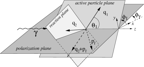
Figure 1: Definition of the coordinate frame in the c.m. system.

We choose as independent variables for the description of this reaction the photon energy $\omega=k$, the momentum of the outgoing active particle $\vec{q}_{1}$ and the spherical angles $\Omega_{p}=(\theta_{p},\phi_{p})$ of the relative momentum $\vec{p}$ of the outgoing meson “2” and nucleon as given by

$$\vec{p}=(M_{p}\vec{q}_{2}-m_{2}\vec{p}_{f})/(M_{p}+m_{2})=(p,\Omega_{p})\,.$$ (1)

The momentum $\vec{p}$ is located in the reaction plane. Then the momenta of the second meson and the outgoing nucleon are fixed. For example, the meson momentum reads

$$\vec{q}_{2}=\vec{p}-\frac{m_{2}}{M_{p}+m_{2}}\,{\vec{q}_{1}}\,.$$ (2)

In the following we will use for the active particle $\vec{q}=(q,\Omega_{q})$ instead of $\vec{q}_{1}$ for convenience.

In Ref. FiA11 the following expression for the $T$-matrix had been derived by expansion of the final state into partial waves

$$T_{m_{f}\mu m_{i}}(\Omega_{p},\Omega_{q}) = e^{i(\mu+m_{i}-m_{f})\phi_{q}}t_{m_{f}\mu m_{i}}(\theta_{p},\,\theta_{q},\,\phi_{pq})\,,$$ (3)

allowing the separation of the $\phi_{q}$-dependence such that the small $t$-matrix elements depend on $\theta_{p}$, $\theta_{q}$, and the relative azimuthal angle $\phi_{pq}=\phi_{p}-\phi_{q}$ only. The spin quantum numbers $\mu$, $m_{i}$, and $m_{f}$ refer to the photon and initial and final nucleon, respectively, where the photon momentum is chosen as quantization axis.

From parity conservation the following symmetry property of the small $t$-matrix elements holds

$$t_{-m_{f}-\mu-m_{i}}(\theta_{p},\,\theta_{q},\,\phi_{pq}) = (-1)^{-m_{f}+\mu+m_{i}}t_{m_{f}\mu m_{i}}(\theta_{p},\,\theta_{q},\,-\phi_{pq})\,.$$ (4)

Thus in contrast to single meson photoproduction on a nucleon, parity conservation does not lead to a reduction of the number of independent amplitudes, as has been noted already in Ref. RoO05 . However, this symmetry will allow one to classify the observables being even or odd under the transformation $\phi_{pq}\to-\phi_{pq}$.

III Observables

In this section we briefly review the main steps for deriving all possible observables for the present reaction as developed for $\pi^{0}\eta$-photoproduction on the nucleon in Ref. FiA11 . It also will allow us to introduce a more compact notation and to correct some misprints in Ref. FiA11 .

The basic quantity is the following general trace with respect to the spin degrees of freedom of photon and initial and final nucleon

$$A_{I^{\prime}M^{\prime}}=c_{kin}tr(T^{\dagger}\tau^{f,[I^{\prime}]}_{M^{\prime}}e^{-iM^{\prime}\phi_{q}}T\rho_{i})\,,$$ (5)

with $c_{kin}$ as a kinematical factor

$$c_{kin}(q,\Omega_{q},\Omega_{pq})=\frac{1}{(2\pi)^{5}}\,\frac{M_{p}^{2}}{E_{i}+p_{i}}\,\frac{1}{8\omega_{\gamma}\omega_{q}}\frac{p_{p}^{2}}{p_{p}(\omega_{2}+E_{f})+\frac{(\vec{q}_{2}+\vec{p}_{f})\cdot\vec{p}_{p}}{p_{p}(M_{p}+m_{2})}(E_{f}m_{2}-\omega_{2}M_{p})}\,,$$ (6)

and where $\rho_{i}$ denotes the density matrix of the initial spin degrees of freedom of photon and nucleon, and $\tau^{f,[I^{\prime}]}_{M^{\prime}}$ a spin operator with respect to the final nucleon spin space (see Ref. FiA11 for details). The trace has the property

$$A_{I^{\prime}M^{\prime}}^{*}=(-)^{M^{\prime}}A_{I^{\prime}-M^{\prime}}\,.$$ (7)

Differential cross section and recoil polarization components are obtained from

$$A_{I^{\prime}M^{\prime}}^{\pm}=\frac{1}{2}\,(A_{I^{\prime}M^{\prime}}\pm(-)^{M^{\prime}}A_{I^{\prime}-M^{\prime}})\,.$$ (8)

Namely, the differential cross section including all possible polarization effects is given by

$$\frac{d^{5}\sigma}{d^{3}qd\Omega_{pq}}=A_{00}^{+}\,,$$ (9)

where $\Omega_{pq}=(\theta_{p},\phi_{q}-\phi_{p})$, and the recoil nucleon polarization components with respect to the active particle frame are given by

$$P_{x}\frac{d^{5}\sigma}{d^{3}qd\Omega_{pq}} = -\sqrt{2}\,A_{11}^{+}=-\sqrt{2}\,\mathrm{Re}\,A_{11}^{+}\,,$$ (10)

$$P_{y}\frac{d^{5}\sigma}{d^{3}qd\Omega_{pq}} = \sqrt{2}\,i\,A_{11}^{-}=-\sqrt{2}\,\mathrm{Im}\,A_{11}^{-}\,,$$ (11)

$$P_{z}\frac{d^{5}\sigma}{d^{3}qd\Omega_{pq}} = A_{10}^{+}\,.$$ (12)

In view of eq. (7), the quantity $A_{I^{\prime}M^{\prime}}^{+}$ is real and $A_{I^{\prime}M^{\prime}}^{-}$ is purely imaginary. Obviously, $A_{I^{\prime}0}^{-}$ vanishes and one has $A_{I^{\prime}0}^{+}=A_{I^{\prime}0}$.

Explicitly the general trace becomes

$$A_{I^{\prime}M^{\prime}} = \frac{1}{2}\,\sum_{IM}P_{I}^{p}\,e^{iM\phi_{qs}}\,d^{I}_{M0}(\theta_{s})\,\sum_{\mu}\Big{[}(1+\mu P^{\gamma}_{c})\,u^{\mu\mu}_{I^{\prime}M^{\prime};IM}-P^{\gamma}_{\ell}\,u^{\mu-\mu}_{I^{\prime}M^{\prime};IM}e^{-2i\mu\phi_{q\gamma}}\Big{]}\,,$$ (13)

where $|P^{\gamma}_{c}|$ and $P^{\gamma}_{\ell}$ describe the degrees of circular and linear polarization, respectively, and $\phi_{q\gamma}=\phi_{q}-\phi_{\gamma}$, where $\phi_{\gamma}$ denotes the angle of maximal linear polarization. With respect to the nucleon polarization parameters $P^{p}_{I}$, one has $P^{p}_{0}=1$, and $P^{p}_{1}$ describes the degree of nucleon polarization along a direction with spherical angles $\Omega_{s}=(\theta_{s},\phi_{s})$ and $\phi_{qs}=\phi_{q}-\phi_{s}$. Furthermore, we have defined

$$u_{I^{\prime}M^{\prime};IM}^{\mu^{\prime}\mu}(q,\,\theta_{q},\,\theta_{p},\,\phi_{pq}) = c_{kin}\,\widehat{I^{\prime}}\widehat{I}\,\sum_{m_{f}m_{f}^{\prime}m_{i}m_{i}^{\prime}}(-1)^{m_{f}^{\prime}-m_{i}}\left(\begin{matrix}\frac{1}{2}&\frac{1}{2}&I^{\prime}\cr m_{f}&-m_{f}^{\prime}&M^{\prime}\cr\end{matrix}\right)\left(\begin{matrix}\frac{1}{2}&\frac{1}{2}&I\cr m_{i}&-m_{i}^{\prime}&-M\cr\end{matrix}\right)$$ (14)

$$\hskip 56.9055pt\times\ t^{*}_{m_{f}^{\prime}\mu^{\prime}m_{i}^{\prime}}(q,\,\theta_{q},\,\theta_{p},\,\phi_{pq})\,t_{m_{f}\mu m_{i}}(q,\,\theta_{q},\,\theta_{p},\,\phi_{pq})\,.$$

These quantities have the following symmetry properties:
(i) for complex conjugation one finds

$$\Big{(}u_{I^{\prime}M^{\prime};IM}^{\mu^{\prime}\mu}(q,\,\theta_{q},\,\theta_{p},\,\phi_{pq})\Big{)}^{*}=(-1)^{M^{\prime}+M}\,u_{I^{\prime}-M^{\prime};I-M}^{\mu\mu^{\prime}}(q,\,\theta_{q},\,\theta_{p},\,\phi_{pq})\,,$$ (15)

(ii) for reversing the sign of the photon helicities $\mu$ and $\mu^{\prime}$ from parity conservation (see eq. (4))

$$u_{I^{\prime}M^{\prime};IM}^{-\mu^{\prime}-\mu}(q,\,\theta_{q},\,\theta_{p},\,\phi_{pq})=(-1)^{I^{\prime}+M^{\prime}+I+M+\mu^{\prime}+\mu}\,u_{I^{\prime}-M^{\prime};I-M}^{\mu^{\prime}\mu}(q_{,}\,\theta_{q},\,\theta_{p},\,-\phi_{pq})\,.$$ (16)

A specific consequence of the symmetry in eq. (15) is that $u_{I^{\prime}0;I0}^{\mu\mu}$ is real. Combining these two properties results in

$$\Big{(}u_{I^{\prime}M^{\prime};IM}^{\mu^{\prime}\mu}(q,\,\theta_{q},\,\theta_{p},\,\phi_{pq})\Big{)}^{*}=(-1)^{I^{\prime}+I+\mu^{\prime}+\mu}\,u_{I^{\prime}M^{\prime};IM}^{-\mu-\mu^{\prime}}(q,\,\theta_{q},\,\theta_{p},-\phi_{pq})\,.$$ (17)

As one will see below, this property leads to the aforementioned classification of the observables.

For the separation of the various types of photon polarization we introduce for $\alpha\in\{0,c,\ell\}$ referring to unpolarized, circularly and linearly polarized radiation, respectively,

$$u^{\alpha}_{I^{\prime}M^{\prime};IM}=\sum_{\mu^{\prime}\mu}\Big{(}(\delta_{\alpha,0}+\mu\,\delta_{\alpha,c})\,\delta_{\mu^{\prime},\mu}-\delta_{\alpha,\ell}\,\delta_{\mu^{\prime},-\mu}e^{-2i\mu^{\prime}\phi_{q\gamma}}\Big{)}u_{I^{\prime}M^{\prime};IM}^{\mu^{\prime}\mu}\,,$$ (18)

or in detail

$$u^{0}_{I^{\prime}M^{\prime};IM} = \sum_{\mu}u_{I^{\prime}M^{\prime};IM}^{\mu\mu}\,,$$ (19)

$$u^{c}_{I^{\prime}M^{\prime};IM} = \sum_{\mu}\mu\,u_{I^{\prime}M^{\prime};IM}^{\mu\mu}\,,$$ (20)

$$u^{\ell}_{I^{\prime}M^{\prime};IM} = -\sum_{\mu}\,e^{-2i\mu\phi_{q\gamma}}\,u_{I^{\prime}M^{\prime};IM}^{\mu-\mu}\,.$$ (21)

These quantities have the symmetry property according to eq. (15)

$$(u^{\alpha}_{I^{\prime}M^{\prime};IM})^{*}=(-)^{M^{\prime}+M}\,u^{\alpha}_{I^{\prime}-M^{\prime};I-M}\,,$$ (22)

which allows one to bring the trace of eq. (5) into the following form

$$A_{I^{\prime}M^{\prime}}=B_{I^{\prime}M^{\prime}}+(-)^{M^{\prime}}\,B_{I^{\prime}-M^{\prime}}^{*}$$ (23)

with

$$B_{I^{\prime}M^{\prime}} = \frac{1}{2}\,\sum_{I=0}^{1}\sum_{M=0}^{I}\frac{P^{p}_{I}}{1+\delta_{M0}}\,e^{iM\phi_{qs}}\,d^{I}_{M0}(\theta_{s})\,\sum_{\alpha\in\{0,c,\ell\}}P_{\alpha}^{\gamma}\,u^{\alpha}_{I^{\prime}M^{\prime};IM}\,.$$ (24)

Now it is useful to introduce the following notation for $\alpha\in\{0,c\}$ and $M\geq 0$

$$v^{0/c}_{I^{\prime}M^{\prime};IM} = \frac{1}{1+\delta_{M0}}\,u^{0/c}_{I^{\prime}M^{\prime};IM}\,.$$ (25)

In view of eq. (22) the $v^{0/c}_{I^{\prime}M^{\prime};IM}$ have the symmetry property

$$(v^{0/c}_{I^{\prime}M^{\prime};IM})^{*}=(-)^{M^{\prime}+M}\,v^{0/c}_{I^{\prime}-M^{\prime};I-M}\,.$$ (26)

Furthermore, for all $M$ we define

$$v^{\ell}_{I^{\prime}M^{\prime};IM} = -u^{1-1}_{I^{\prime}M^{\prime};IM}\,$$ (27)

and use according to eq. (15)

$$u^{-11}_{I^{\prime}M^{\prime};IM}=-(-)^{M^{\prime}+M}\,v^{\ell\,*}_{I^{\prime}-M^{\prime};I-M}\,.$$ (28)

With the help of the combined symmetry of eq. (17) one finds the following behaviour under the transformation $\phi_{pq}\to-\phi_{pq}$

$$v^{0/\ell}_{I^{\prime}M^{\prime};IM}(q_{,}\,\theta_{q},\,\theta_{p},\,-\phi_{pq}) = (-)^{I^{\prime}+I}(v^{0/\ell}_{I^{\prime}M^{\prime};IM}(q_{,}\,\theta_{q},\,\theta_{p},\,\phi_{pq}))^{*}\,,$$ (29)

$$v^{c}_{I^{\prime}M^{\prime};IM}(q_{,}\,\theta_{q},\,\theta_{p},\,-\phi_{pq}) = -(-)^{I^{\prime}+I}(v^{c}_{I^{\prime}M^{\prime};IM}(q_{,}\,\theta_{q},\,\theta_{p},\,\phi_{pq}))^{*}\,.$$ (30)

In view of the fact that real and imaginary parts of $v^{\alpha}_{I^{\prime}M^{\prime};IM}$ represent the observables (see below), this property allows the classification of them into even and odd with respect to this transformation.

Finally, one obtains

$$B_{I^{\prime}M^{\prime}} = \frac{1}{2}\,\sum_{I=0}^{1}\sum_{M=0}^{I}P^{p}_{I}\,e^{iM\phi_{qs}}\,d^{I}_{M0}(\theta_{s})\,\Big{(}\sum_{\alpha\in\{0,c\}}P_{\alpha}^{\gamma}\,v^{\alpha}_{I^{\prime}M^{\prime};IM}$$ (31)

$$\hskip 56.9055pt+e^{-2i\phi_{q\gamma}}\,v^{\ell}_{I^{\prime}M^{\prime};IM}+(-)^{M^{\prime}+M}\,e^{2i\phi_{q\gamma}}\,v^{\ell\,*}_{I^{\prime}-M^{\prime};I-M}\Big{)}\,.$$

For the quantities in eq. (8) one finds

$$A^{+}_{I^{\prime}M^{\prime}} = \mathrm{Re}\,(B_{I^{\prime}M^{\prime}}+(-)^{M^{\prime}}\,B_{I^{\prime}-M^{\prime}})\,,$$ (32)

$$A^{-}_{I^{\prime}M^{\prime}} = i\,\mathrm{Im}\,(B_{I^{\prime}M^{\prime}}+(-)^{M^{\prime}}\,B_{I^{\prime}-M^{\prime}})\,.$$ (33)

Thus one obtains for the differential cross section and the recoil polarization according to eqs. (9) through (12)

$$\frac{d^{5}\sigma}{d^{3}qd\Omega_{pq}} = 2\,\mathrm{Re}\,B_{00}\,,$$ (34)

$$P_{x}\frac{d^{5}\sigma}{d^{3}qd\Omega_{pq}} = -\sqrt{2}\,\mathrm{Re}\,(B_{11}-B_{1-1})\,,$$ (35)

$$P_{y}\frac{d^{5}\sigma}{d^{3}qd\Omega_{pq}} = -\sqrt{2}\,\mathrm{Im}\,(B_{11}+B_{1-1})\,,$$ (36)

$$P_{z}\frac{d^{5}\sigma}{d^{3}qd\Omega_{pq}} = 2\,\mathrm{Re}\,B_{10}\,.$$ (37)

Now we will proceed to list explicit expressions for the differential cross section and the recoil polarization of the emerging nucleon determining the various observables of this reaction.

III.1 Differential cross section

For convenience we introduce

$$U_{IM}^{\alpha} = v_{00;IM}^{\alpha}$$ (38)

and separate real and imaginary parts according to

$$U_{IM}^{\alpha} = T_{IM}^{\alpha}+i\,S_{IM}^{\alpha}$$ (39)

for $\alpha\in\{0,c,\ell\}$. One should note that $S_{I0}^{0}$ and $S_{I0}^{c}$ vanish according to eq. (26). In view of eqs. (29) and (30) one finds as symmetry property under the transformation $\phi_{pq}\to-\phi_{pq}$

$$U_{IM}^{\alpha}(-\phi_{pq})=(-)^{I+\delta_{\alpha,c}}\,(U_{IM}^{\alpha}(\phi_{pq}))^{*}\,,$$ (40)

i.e. $T_{IM}^{\alpha}$ is symmetric for $I=0$ and $\alpha\in\{0,\ell\}$, and for $I=1$ and $\alpha=c$, and antisymmetric for $I=1$ and $\alpha\in\{0,\ell\}$, and for $I=0$ and $\alpha=c$, whereas the $S_{IM}^{\alpha}$’s have just the opposite behavior.

Then one obtains explicitly for the differential cross section with inclusion of beam and target polarization effects

$$\frac{d^{5}\sigma(P^{\gamma}_{c},P^{\gamma}_{\ell},P^{p}_{1})}{d^{3}qd\Omega_{pq}} = \frac{d^{5}\sigma_{0}}{d^{3}qd\Omega_{pq}}\Big{(}1+P^{\gamma}_{c}\,\Sigma^{c}+P^{\gamma}_{\ell}\,\Sigma^{\ell}(\phi_{q\gamma})$$ (41)

$$\hskip 56.9055pt+P^{p}_{1}\,\Big{[}\Sigma^{p0}(\theta_{s},\phi_{qs})+P^{\gamma}_{c}\,\Sigma^{pc}(\theta_{s},\phi_{qs})+P^{\gamma}_{\ell}\,\Sigma^{p\ell}(\theta_{s},\phi_{qs},\phi_{q\gamma})\Big{]}\Big{)}\,,$$

where the unpolarized differential cross section is given by

$$\frac{d^{5}\sigma_{0}}{d^{3}qd\Omega_{pq}} = T^{0}_{00}\,.$$ (42)

Furthermore, one has beam asymmetries for circular and linear photon polarization

$$\Sigma^{c}\,T^{0}_{00} = T^{c}_{00}\,,$$ (43)

$$\Sigma^{\ell}(\phi_{q\gamma})\,T^{0}_{00} = T^{\ell}_{00}\,\cos{2\phi_{q\gamma}}+S^{\ell}_{00}\,\sin{2\phi_{q\gamma}}\,,$$ (44)

target asymmetry for a polarized target proton but unpolarized photons

$$\Sigma^{p0}(\theta_{s},\phi_{qs})\,T^{0}_{00} = \cos{\theta_{s}}\,T^{0}_{10}-\frac{\sin\theta_{s}}{\sqrt{2}}\,\Big{(}\cos\phi_{qs}\,T^{0}_{11}-\sin\phi_{qs}\,S^{0}_{11}\Big{)}\,,$$ (45)

and beam-target asymmetries for polarized radiation and an oriented target

$$\Sigma^{pc}(\theta_{s},\phi_{qs})\,T^{0}_{00} = \cos{\theta_{s}}\,T^{c}_{10}-\frac{\sin\theta_{s}}{\sqrt{2}}\,\Big{(}\cos\phi_{qs}\,T^{c}_{11}\,-\sin\phi_{qs}\,S^{c}_{11}\Big{)}\,,$$ (46)

$$\Sigma^{p\ell}(\theta_{s},\phi_{qs},\phi_{q\gamma})\,T^{0}_{00} = \cos{\theta_{s}}\,\Big{(}\cos{2\phi_{q\gamma}}\,T^{\ell}_{10}+\sin{2\phi_{q\gamma}\,S^{\ell}_{10}}\Big{)}$$ (47)

$$-\frac{\sin\theta_{s}}{\sqrt{2}}\,\Big{(}\cos\phi_{qs}\Big{[}\cos 2\phi_{q\gamma}\,(T^{\ell}_{11}-T^{\ell}_{1-1})+\sin 2\phi_{q\gamma}\,(S^{\ell}_{11}-S^{\ell}_{1-1})\Big{]}$$

$$+\sin\phi_{qs}\,\Big{[}\sin 2\phi_{q\gamma}\,(T^{\ell}_{11}+T^{\ell}_{1-1})-\cos 2\phi_{q\gamma}\,(S^{\ell}_{11}+S^{\ell}_{1-1})\Big{]}\Big{)}\,.$$

The $T^{\alpha}_{IM}$ and $S^{\alpha}_{IM}$ constitute all possible observables of the differential cross section. For $\alpha\in\{0,c\}$ one has for each case four observables, namely $T^{0/c}_{00},T^{0/c}_{10},T^{0/c}_{11}$ and $S^{0/c}_{11}$, and for $\alpha=\ell$ eight ones, $T^{\ell}_{IM}$ and $S^{\ell}_{IM}$ for $I=0,1$ and $M=-I,\dots,I$. Altogether one finds 16 observables for the differential cross section. Besides one unpolarized observable, the unpolarized differential cross section, one has six single polarization and nine double polarization observables. They can be separated by appropriate choices of the polarization parameters and angles.

III.2 Recoil Polarization

Now we turn to the corresponding expressions for the recoil polarization of the outgoing nucleon. The three components are determined by $B_{1M}$ according to eqs. (35) through (37). For convenience we introduce for $\alpha\in\{0,c,\ell\}$

$$R_{IM}^{x,\alpha} = -\frac{1}{\sqrt{2}}\,(v^{\alpha}_{11;IM}-v^{\alpha}_{1-1;IM})\,$$ (48)

$$R_{IM}^{y,\alpha} = \frac{i}{\sqrt{2}}\,(v^{\alpha}_{11;IM}+v^{\alpha}_{1-1;IM})\,$$ (49)

$$R_{IM}^{z,\alpha} = v^{\alpha}_{10;IM}\,,$$ (50)

and separate into real and imaginary parts

$$R_{IM}^{x_{i},\alpha}=P_{IM}^{x_{i},\alpha}+i\,Q_{IM}^{x_{i},\alpha}\,.$$ (51)

One should note that the $R_{I0}^{x_{i},0/c}$ are real. Furthermore for $\alpha\in\{0,c\}$, $R_{IM}^{x_{i},0/c}$ appear with $M\geq 0$ only.

As symmetry property under the transformation $\phi_{pq}\to-\phi_{pq}$ one obtains

$$R_{IM}^{x_{i},\alpha}(-\phi_{pq})=-(-)^{I+\delta_{\alpha,c}+\delta_{x_{i},y}}(R_{IM}^{x_{i},\alpha}(\phi_{pq}))^{*}\,,$$ (52)

which means $P_{IM}^{x_{i},\alpha}$ is symmetric and $Q_{IM}^{x_{i},\alpha}$ antisymmetric for $x_{i}=x,z$ and either $I=1$ and $\alpha\in\{0,\ell\}$ or $I=0$ and $\alpha=c$, furthermore for $x_{i}=y$ and either $I=0$ and $\alpha\in\{0,\ell\}$ or $I=1$ and $\alpha=c$. In all other cases one has just the opposite behavior.

For later purpose we introduce also the spherical components $\mu=0,\pm 1$

$$R_{IM}^{\mu,\alpha}=\delta_{\mu,0}\,R_{IM}^{z,\alpha}-\frac{\mu}{\sqrt{2}}\,(R_{IM}^{x,\alpha}+i\,\mu\,R_{IM}^{y,\alpha})=v^{\alpha}_{1\mu;IM}\,.$$ (53)

For $\alpha\in\{0,c\}$ one finds from the symmetry property in eq. (26)

$$R_{IM}^{\mu,\alpha\,*}=(-)^{\mu+M}\,R_{I-M}^{-\mu,\alpha}\,,$$ (54)

From which follows in particular for $M=0$

$$R_{I0}^{\mu,0/c\,*}=(-)^{\mu}\,R_{I0}^{-\mu,0/c}\,.$$ (55)

Thus one obtains finally for the recoil polarization component $P_{x_{i}}$

$$P_{x_{i}}\frac{d^{5}\sigma(P^{\gamma}_{c},P^{\gamma}_{\ell},P^{p}_{1})}{d^{3}qd\Omega_{pq}} = \frac{d\sigma_{0}}{d^{3}qd\Omega_{pq}}\Big{(}P^{0}_{x_{i}}+P^{\gamma}_{c}\,P^{c}_{x_{i}}+P^{\gamma}_{\ell}\,P^{\ell}_{x_{i}}(\phi_{q\gamma})$$ (56)

$$\hskip 42.67912pt+P^{p}_{1}\,\Big{[}P^{p0}_{x_{i}}(\theta_{s},\phi_{qs})+P^{\gamma}_{c}\,P^{pc}_{x_{i}}(\theta_{s},\phi_{qs})+P^{\gamma}_{\ell}\,P^{p\ell}_{x_{i}}(\theta_{s},\phi_{qs},\phi_{q\gamma})\Big{]}\Big{)}$$

with recoil polarizations for unpolarized beam and target

$$P^{0}_{x_{i}}\,T^{0}_{00} = P^{x_{i},0}_{00}\,,$$ (57)

as well as beam asymmetries for circularly and linearly polarized photons

$$P^{c}_{x_{i}}\,T^{0}_{00} = P^{x_{i},c}_{00}\,,$$ (58)

$$P^{\ell}_{x_{i}}(\phi_{q\gamma})\,T^{0}_{00} = \cos{2\phi_{q\gamma}}\,P^{x_{i},\ell}_{00}+\sin{2\phi_{q\gamma}},Q^{x_{i},\ell}_{00}\,,$$ (59)

target asymmetry for a polarized proton target

$$P^{p0}_{x_{i}}(\theta_{s},\phi_{qs})\,T^{0}_{00} = \cos{\theta_{s}}\,P^{x_{i},0}_{10}-\frac{\sin\theta_{s}}{\sqrt{2}}\,\Big{(}\cos\phi_{qs}\,P^{x_{i},0}_{11}-\sin\phi_{qs}\,Q^{x_{i},0}_{11}\Big{)}\,,$$ (60)

and beam-target asymmetries

$$P^{pc}_{x_{i}}(\theta_{s},\phi_{qs})\,T^{0}_{00} = \cos{\theta_{s}}\,P^{x_{i},c}_{10}-\frac{\sin\theta_{s}}{\sqrt{2}}\,\Big{(}\cos\phi_{qs}\,P^{x_{i},c}_{11}-\sin\phi_{qs}\,Q^{x_{i},c}_{11}\Big{)}\,,$$ (61)

$$P^{p\ell}_{x_{i}}(\theta_{s},\phi_{qs},\phi_{q\gamma})\,T^{0}_{00} = \cos{\theta_{s}}\Big{(}\cos{2\phi_{q\gamma}}\,P^{x_{i},\ell}_{10}+\sin{2\phi_{q\gamma}\,Q^{x_{i},\ell}_{10}}\Big{)}$$ (62)

$$-\frac{\sin\theta_{s}}{\sqrt{2}}\,\Big{(}\cos\phi_{qs}\,\Big{[}\cos 2\phi_{q\gamma}\,(P^{x_{i},\ell}_{11}-P^{x_{i},\ell}_{1-1})+\sin 2\phi_{q\gamma}\,(Q^{x_{i},\ell}_{11}-Q^{x_{i},\ell}_{1-1})\Big{]}$$

$$\hskip 28.45274pt-\sin\phi_{qs}\,\Big{[}\cos 2\phi_{q\gamma}(Q^{x_{i},\ell}_{11}+Q^{x_{i},\ell}_{1-1})-\sin 2\phi_{q\gamma}(P^{x_{i},\ell}_{11}+P^{x_{i},\ell}_{1-1})\Big{]}\Big{)}\,,\,$$

constituting 48 observables for the recoil polarization components. Of these three are single, eighteen double and twenty seven triple polarization observables. They can be separated by appropriate choices of the polarization parameters and angles.

Together with the 16 observables of the differential cross section this gives a total number of 64 observables which number coincides with the maximal number of linearly independent quadratic hermitean forms one can form from eight independent complex amplitudes. On the other hand the eight complex amplitudes with one arbitrary phase constitute fifteen independent parameters. Thus a minimal set of observables for the determination of these amplitudes should comprise at least fifteen observables, a so-called complete set. Although the above 64 observables are linearly independent there exist quadratic relations between them, and thus it is a challenge to find minimal (complete) sets of observables.

III.3 Observables in terms of $t$-matrix elements

In view of a detailed determination of the $t$-matrix elements from observables it is useful to have explicit expressions of the latter as linear forms in the bilinear terms ${\cal T}_{j^{\prime}j}=t_{j^{\prime}}^{*}t_{j}$. Here $j=\{m_{f}\mu\,m_{i}\}$ numbers the $t$-matrix elements according to Table 1.

Table 1: Enumeration $j$ of the small $t_{j}$-matrix elements with $j=\{m_{f}\mu\,m_{i}\}$.

$j$	1	2	3	4	5	6	7	8
$m_{f}$	$1/2$	$-1/2$	$1/2$	$-1/2$	$1/2$	$-1/2$	$1/2$	$-1/2$
$\mu$	$1$	$1$	$-1$	$-1$	$1$	$1$	$-1$	$-1$
$m_{i}$	$1/2$	$1/2$	$1/2$	$1/2$	$-1/2$	$-1/2$	$-1/2$	$-1/2$

The basic quantities in which all observables are expressed are the $v^{\alpha}_{I^{\prime}M^{\prime};IM}$ as defined in eqs. (25) and (27)

$$v^{\alpha}_{I^{\prime}M^{\prime};IM}=c_{kin}\,\sum_{j^{\prime}j}\,{C}^{I^{\prime}M^{\prime};IM}_{j^{\prime}j}\,f^{\alpha,M}_{j^{\prime}j}\,{\cal T}_{j^{\prime}j}$$ (63)

with

$${C}^{I^{\prime}M^{\prime};IM}_{j^{\prime}j} = {C}^{I^{\prime}M^{\prime};IM}_{\{m_{f}^{\prime}\mu^{\prime}m_{i}^{\prime}\}\{m_{f}\mu\,m_{i}\}}$$ (64)

$$= (-)^{m_{f}^{\prime}-m_{i}}\,\widehat{I}^{\prime}\widehat{I}\left(\begin{matrix}\frac{1}{2}&\frac{1}{2}&I^{\prime}\cr m_{f}&-m_{f}^{\prime}&M^{\prime}\cr\end{matrix}\right)\left(\begin{matrix}\frac{1}{2}&\frac{1}{2}&I\cr m_{i}&-m_{i}^{\prime}&-M\cr\end{matrix}\right)\,,$$

and

$$f^{\alpha,M}_{j^{\prime}j}=f^{\alpha}_{\{m_{f}^{\prime}\mu^{\prime}m_{i}^{\prime}\}\{m_{f}\mu\,m_{i}\}}=(\delta_{\alpha,0}+\mu\,\delta_{\alpha,c})\frac{\delta_{\mu^{\prime}\mu}}{1+\delta_{M,0}}-\delta_{\alpha,\ell}\delta_{\mu^{\prime},1}\delta_{\mu,-1}\,.$$ (65)

Evaluation of the observables in eqs. (38) and (48) through (50) yields then the expressions listed in appendix A.

III.4 Bilinear $T$-matrix expressions in term of observables

With respect to the question of a minimal set of observables needed for a complete analysis we now will derive explicit expressions for ${\cal T}_{j^{\prime}j}$ in terms of observables. The starting point is eq. (14) for $u^{\mu^{\prime}\mu}_{I^{\prime}M^{\prime};IM}$, which are the basic quantities for all observables in terms of the $t$-matrix elements. It is easily inverted yielding with $j^{\prime}=\{m_{f}^{\prime}\mu^{\prime}m_{i}^{\prime}\}$ and $j=\{m_{f}\mu\,m_{i}\}$

$${\cal T}_{j^{\prime}j}=\frac{1}{c_{kin}}\,\sum_{I^{\prime}M^{\prime}IM}{C}^{I^{\prime}M^{\prime};IM}_{j^{\prime}j}\,u^{\mu^{\prime}\mu}_{I^{\prime}M^{\prime};IM}\delta_{M,m_{i}-m_{i}^{\prime}}\delta_{M^{\prime},m_{f}^{\prime}-m_{f}}\,.$$ (66)

where ${C}^{I^{\prime}M^{\prime};IM}_{j^{\prime}j}$ is given in eq. (64). The next step is to express the $u^{\mu^{\prime}\mu}_{I^{\prime}M^{\prime};IM}$ by the quantities $v^{\alpha}_{I^{\prime}M^{\prime};IM}$. According to the eqs. (25), (27) and (28) one obtains

$$u^{\mu^{\prime}\mu}_{I^{\prime}M^{\prime};IM} = \frac{1+\delta_{M,0}}{2}\,\delta_{\mu^{\prime},\mu}\,(v^{0}_{I^{\prime}M^{\prime};IM}+\mu\,v^{c}_{I^{\prime}M^{\prime};IM})$$ (67)

$$-\delta_{\mu^{\prime},1}\,\delta_{\mu,-1}\,v^{\ell}_{I^{\prime}M^{\prime};IM}-\delta_{\mu^{\prime},-1}\delta_{\mu,1}(-)^{M^{\prime}+M}\,v^{\ell\,*}_{I^{\prime}-M^{\prime};I-M}\,.$$

As final step we relate $v^{\alpha}_{I^{\prime}M^{\prime};IM}$ to the various observables of the differential cross section and the recoil polarization components using eqs. (38) and (53)

$$v^{0/c}_{I^{\prime}M^{\prime};IM} = \delta_{I^{\prime},0}\,(\delta_{M,0}\,T^{0/c}_{I0}+\delta_{M,1}\,U^{0/c}_{11}-\delta_{M,-1}\,U^{0/c\,*}_{11})$$ (68)

$$+\delta_{I^{\prime},1}\,(\delta_{M,0}\,P^{M^{\prime},0/c}_{I0}+\delta_{M,1}\,R^{M^{\prime},0/c}_{11}-\delta_{M,-1}\,(-)^{M^{\prime}}R^{M^{\prime},0/c\,*}_{11})\,,$$

$$v^{\ell}_{I^{\prime}M^{\prime};IM} = \delta_{I^{\prime},0}\,U^{\ell}_{IM}+\delta_{I^{\prime},1}\,R^{M^{\prime},\ell}_{IM}\,.$$ (69)

Thus one obtains for ${\cal T}_{j^{\prime}j}$ in terms of observables

$${\cal T}_{j^{\prime}j} = \frac{1}{c_{kin}}\,\sum_{I^{\prime}M^{\prime}IM}{C}^{I^{\prime}M^{\prime};IM}_{j^{\prime}j}\,\delta_{M,m_{i}-m_{i}^{\prime}}\delta_{M^{\prime},m_{f}^{\prime}-m_{f}}$$ (70)

$$\times\Big{\{}\frac{1+\delta_{M,0}}{2}\,\delta_{\mu^{\prime},\mu}\,\Big{[}\delta_{I^{\prime},0}\,\Big{(}\delta_{M,0}\,(T^{0}_{I0}+\mu\,T^{c}_{I0})+\delta_{M,1}\,(U^{0}_{11}+\mu\,U^{c}_{11})-\delta_{M,-1}\,(U^{0\,*}_{11}+\mu\,U^{c\,*}_{11})\Big{)}$$

$$+\delta_{I^{\prime},1}\,\Big{(}\delta_{M,0}\,(P^{M^{\prime},0}_{I0}+\mu\,P^{M^{\prime},c}_{I0})+\delta_{M,1}\,(R^{M^{\prime},0}_{11}+\mu\,R^{M^{\prime},c}_{11})-\delta_{M,-1}\,(-)^{M^{\prime}}(R^{M^{\prime},0\,*}_{11}+\mu\,R^{M^{\prime},c\,*}_{11})\Big{)}\Big{]}$$

$$-\delta_{\mu^{\prime},1}\,\delta_{\mu,-1}\,\Big{[}\delta_{I^{\prime},0}\,U^{\ell}_{IM}+\delta_{I^{\prime},1}\,R^{M^{\prime},\ell}_{IM}\Big{]}-\delta_{\mu^{\prime},-1}\delta_{\mu,1}(-)^{M^{\prime}+M}\,\Big{[}\delta_{I^{\prime},0}\,U^{\ell\,*}_{I-M}+\delta_{I^{\prime},1}\,R^{-M^{\prime},\ell\,*}_{I-M}\Big{]}\Big{\}}\,.$$

A listing of the resulting expressions is given in appendix B, where also a graphical representation is introduced.

IV On complete sets of polarization observables

In this section we will consider two strategies for finding a minimal complete set of observables allowing the determination of all $t$-matrix elements up to an arbitrary phase. The first one was developed in Ref. ArLT98 and applied to the analysis of deuteron electro- and photodisintegration in Ref. ArLT00 . Recently, it has also been applied to the analysis of photoproduction of two pseudoscalar mesons on a nucleon within a truncated partial wave approach FiA13 . The second method was developed and applied in Ref. ArLT00 again to deuteron electro- and photodisintegration.

IV.1 First Method

We start with a brief description of the salient features of this method as reported in Refs. ArLT98 ; ArLT00 . The idea is as follows: Given for an $n$-dimensional t-matrix a minimal set of $m=2n-1$ observables

$${\cal O}^{\alpha}=\sum_{i,j=1,n}t_{i}^{*}H^{\alpha}_{ij}t_{j}\,,\quad\alpha=1,\dots,m\,,$$ (71)

constituting a set of $m$ hermitean quadratic forms in the $t$-matrix elements, of which $t_{i_{0}}$ is chosen to be real, then a necessary condition for the invertability is that the associated Jacobian is nonvanishing in the vicinity of a solution. The evaluation of the Jacobian then leads to the following condition: For each of the $n\times n$ matrices

$$H^{\alpha}_{ij}=A^{\alpha}_{ij}+i\,B^{\alpha}_{ij}\,,$$ (72)

associated with the observable ${\cal O}^{\alpha}$, where $A^{\alpha}_{ij}$ is a real symmetric and $B^{\alpha}_{ij}$ a real antisymmetric matrix, one constructs a $m\times m$-matrix

$$\widetilde{H}^{\alpha}=\left(\begin{matrix}A^{\alpha}&(\widetilde{B}^{\alpha})^{T}\cr\widetilde{B}^{\alpha}&\widehat{A}^{\alpha}\cr\end{matrix}\right)\,.$$ (73)

Here, $\widehat{A}^{\alpha}$ is obtained from $A^{\alpha}$ by canceling the $i_{0}$-th row and column, and $\widetilde{B}^{\alpha}$ from $B^{\alpha}$ by canceling the $i_{0}$-th row. For all possible sets $\{k_{1},\dots,k_{m}\}$ with $k_{\alpha}\in\{1,\dots,m\}$ one builds by choosing from $\widetilde{H}^{\alpha}$ the $k_{\alpha}$-th column the matrix

$$\widetilde{W}(k_{1},\dots,k_{m})=\left(\begin{array}[]{ccc}\widetilde{H}^{1}_{1k_{1}}&\cdots&\widetilde{H}^{m}_{1k_{m}}\\ \vdots&&\vdots\\ \widetilde{H}^{1}_{mk_{1}}&\cdots&\widetilde{H}^{m}_{mk_{m}}\end{array}\right)\,.$$ (74)

One should note that the $k_{\alpha}$ need not be different. Now the condition is that at least one of the determinants of $\widetilde{W}(k_{1},\dots,k_{m})$ is nonvanishing. This condition, however, is in general not sufficient in case that several of these determinants are nonvanishing. If only one determinant is nonvanishing, than this condition is also sufficient. Moreover, one might encounter quadratic ambiguities in the solution.

Turning now to the present reaction, one readily notes that, according to the explicit listing of all observables in terms of the $t$-matrix elements, all matrices $H^{\alpha}_{ij}$ have a simple structure. They are either real symmetric, i.e. of type $A^{\alpha}$, or imaginary antisymmetric, i.e. of type $iB^{\alpha}$. Moreover, they have for each row and each column at most only one nonvanishing entry. Thus the associated matrices $\widetilde{H}^{\alpha}$ are easily constructed and have a similar structure. For this reason, it turns out, that for any selection of 15 observables the above criterion is fulfilled. However, in all cases one can find more than one non-vanishing determinant.

As an example, we have selected the following set of fifteen observables, guided by their representation in terms of ${\cal T}_{j^{\prime}j}$ (see appendix B): $T^{0}_{00}$, $U^{0}_{11}=T^{0}_{11}+i\,S^{0}_{11}$, $U^{c}_{11}=T^{c}_{11}+i\,S^{c}_{11}$, $R^{z,0}_{11}=P^{z,0}_{11}+i\,Q^{z,0}_{11}$, $R^{z,c}_{11}=P^{z,c}_{11}+i\,Q^{z,c}_{11}$, $U^{\ell}_{00}=T^{\ell}_{00}+i\,S^{\ell}_{00}$, $U^{\ell}_{10}=T^{\ell}_{10}+i\,S^{\ell}_{10}$, $P^{x+iy,0}_{00}=P^{x,0}_{00}+i\,P^{y,0}_{00}$. This set contains one unpolarized observable, four single, eight double and two triple polarization observables.

In appendix C it is shown, how all seven matrix elements $t_{2},\dots,t_{8}$ can be expressed by $t_{1}$ and the chosen observables. In detail one finds $t_{j}=\frac{\sigma_{j}}{t_{1}^{*}}$ for $j=2,3,5,8$ with

$$\sigma_{2}=c_{12}\,,\quad\sigma_{3}=c_{13}\,,\quad\sigma_{5}=c_{51}^{*}\,,\quad\sigma_{8}=\frac{c_{12}\,c_{84}^{*}}{c_{24}^{*}}\,,$$ (75)

and $t_{j}=\tau_{j}\,t_{1}$ for $j=4,6,7$ with

$$\tau_{4}=\frac{c_{24}}{c_{12}^{*}}\,,\quad\tau_{6}=\frac{c_{62}^{*}}{c_{12}^{*}}\,,\quad\tau_{7}=\frac{c_{73}^{*}}{c_{13}^{*}}\,.$$ (76)

The various complex constants $c_{ij}$, expressed in terms of observables, may be found in the appendix C. The constants $c_{12}$ and $c_{13}$ contain quadratic ambiguities.

Finally, the remaining matrix element $t_{1}$ is obtained from the unpolarized differential cross section in eq. (C1), i.e.

$$c_{0} = 4\,c_{kin}\,T^{0}_{00}=a_{1}\,|t_{1}|^{2}+\frac{b_{1}}{|t_{1}|^{2}}\,,$$ (77)

with

$$a_{1}=1+|\tau_{4}|^{2}+|\tau_{6}|^{2}+|\tau_{8}|^{2}\,,\quad b_{1}=|\sigma_{2}|^{2}+|\sigma_{3}|^{2}+|\sigma_{5}|^{2}+\sigma_{8}|^{2}\,.$$ (78)

It has as solution

$$|t_{1}|^{2} = \frac{1}{2a_{1}}\Big{(}c_{0}\pm\sqrt{(c_{0})^{2}-4\,a_{1}\,b_{1}}\Big{)}\,,$$ (79)

introducing a third ambiguity. However, it turns out, that some of these ambiguities are eliminated by the condition

$$(c_{0})^{2}-4\,a_{1}\,b_{1}\geq 0\,.$$ (80)

Indeed, taking a specific numerical example, we found, that only the ambiguity of eq. (79) remains, which is easily resolved by selecting one additional observables, for example, $P^{z,0}_{00}$. Altogether, these sixteen observables allow one to determine uniquely the eight complex $t$-matrix elements.

IV.2 Second Method

Another possibility of constructing a complete set of polarization observables is to study first the representation of the bilinear $t$-matrix products ${\cal T}_{j^{\prime}j}$ in terms of observables. In appendix B we have listed explicit expressions and also outlined a graphical representation as devised in Ref. ArLT00 . It turns out that they can be divided into groups according to the participating observables. This division is unique and there is no overlap of observables between different groups. Altogether one obtains eight groups, one containing the eight diagonal terms $|t_{j}|^{2}$ with eight observables, and seven groups for the 28 interference terms, each containing four interference terms with eight observables.

One can now try to combine the various interference terms in a complete chain of interference terms $t_{j_{1}j_{2}},\dots,t_{j_{n-1}j_{n}}$ with $(j_{1},\dots,j_{n})$ as a permutation of $(1,\dots,n)$. The ideal case is, that the participating observables of such a chain plus an additional independent observable constitute a minimal complete set, i.e. are sufficient for the determination of all $t$-matrix elements. However, such an ideal situation is seldom found. In fact, for the present reaction this is not the case as the graphical representations of the various groups in appendix B demonstrate. However, we can utilize these representations by combining various groups in order to construct such a chain. In such combinations one finds closed loops which constitute higher order relations between observables, which then can be used for the elimination of superfluous observables.

For example, considering the observables of the differential cross section and recoil polarization component $P_{z}$ and combining group “A1”, containing $U^{0}_{11}$, $U^{c}_{11}$, $R^{z,0}_{11}$, and $R^{z,c}_{11}$, with group “B”, containing $U^{\ell}_{00}$, $U^{\ell}_{10}$, $R^{z,\ell}_{00}$, and $R^{z,\ell}_{10}$, one obtains the pattern displayed in Fig. 2. Here one can distinguish two connected groups: (i) group “I” with the matrix elements $t_{1}$, $t_{3}$, $t_{5}$, and $t_{7}$, and (ii) group “II” with the matrix elements of even number $t_{2}$, $t_{4}$, $t_{6}$, and $t_{8}$. For each group the matrix elements are connected by interference terms building two four-point closed loops, namely “1-3-7-5-1” and “2-4-8-6-2”.

Figure 2: Combined graphical representation of the groups “A1” (solid) and “B” (dashed).

Thus for both groups all $t$-matrix elements terms can be expressed relative to one matrix element, for example in the first group “I” with respect to $t_{1}$, i.e.

$$t_{3}=\frac{{\cal T}_{13}}{t_{1}^{*}}\,,\quad t_{5}=\frac{{\cal T}_{15}}{t_{1}^{*}}\,,\quad t_{7}=\frac{{\cal T}_{57}}{{\cal T}_{51}}\,t_{1}=\frac{{\cal T}_{37}}{{\cal T}_{31}}\,t_{1}\,.$$ (81)

The last equation yields because of the closed loop “1-3-7-5-1” a quadratic relation between observables

$${\cal T}_{31}{\cal T}_{57} = {\cal T}_{37}{\cal T}_{51}\,,$$ (82)

or explicitly in terms of observables

$${2}\,(U^{\ell}_{00}+U^{\ell}_{10}+R^{z,\ell}_{00}+R^{z,\ell}_{10})^{*}(U^{\ell}_{00}-U^{\ell}_{10}+R^{z,\ell}_{00}-R^{z,\ell}_{10}) = (U^{0}_{11}-U^{c}_{11}+R^{z,0}_{11}-R^{z,c}_{11})^{*}$$ (83)

$$\times(U^{0}_{11}+U^{c}_{11}+R^{z,0}_{11}+R^{z,c}_{11})\,.$$

Similarly one can express all matrix elements of the second group “II” in terms of say $t_{2}$ according to

$$t_{4}=\frac{{\cal T}_{24}}{t_{2}^{*}}\,,\quad t_{6}=\frac{{\cal T}_{26}}{t_{2}^{*}}\,,\quad t_{8}=\frac{{\cal T}_{48}}{{\cal T}_{42}}\,t_{2}=\frac{{\cal T}_{68}}{{\cal T}_{62}}\,t_{2}\,.$$ (84)

Again, one finds from the last equation a quadratic relation from the second closed loop “2-4-8-6-2”

$${\cal T}_{42}{\cal T}_{68} = {\cal T}_{48}{\cal T}_{62}\,,$$ (85)

and in terms of observables

$${2}\,(U^{\ell}_{00}+U^{\ell}_{10}-R^{z,\ell}_{00}-R^{z,\ell}_{10})^{*}(U^{\ell}_{00}-U^{\ell}_{10}-R^{z,\ell}_{00}+R^{z,\ell}_{10}) = (U^{0}_{11}-U^{c}_{11}-R^{z,0}_{11}+R^{z,c}_{11})^{*}$$ (86)

$$\times(U^{0}_{11}+U^{c}_{11}-R^{z,0}_{11}-R^{z,c}_{11})\,.$$

Formally this relation can be obtained from eq. (83) by the substitutions $R^{z,\ell}_{00/10}\to-R^{z,\ell}_{00/10}$ and $R^{z,0/c}_{11}\to-R^{z,0/c}_{11}$. These two relations can be utilized for the elimination of the four triple polarization observables contained in $R^{z,c}_{11}$ and $R^{z,\ell}_{10}$. This is shown in appendix D. The remaining group contains only single and double polarization observables.

Thus, the matrix elements with odd numbers $t_{3}$, $t_{5}$, and $t_{7}$ can be expressed by the observables of “A1” and “B” and $t_{1}$, while the ones with even numbers $t_{4}$, $t_{6}$, and $t_{8}$ can be expressed by the same observables and $t_{2}$. Of the sixteen observables of “A1” and “B” four, namely $R^{z,c}_{11}$ and $R^{z,\ell}_{10}$, are eliminated, leaving twelve observables.

Obviously, for a complete determination one needs an interference term connecting these two groups, i.e. an interference term ${\cal T}_{j^{\prime}j}$ with $j^{\prime}$ even and $j$ odd or vice versa. Since the interference terms given in terms of observables of the differential cross section and the recoil polarization component $P_{z}$ involve $t$-matrix elements of either both even or both odd numbers one has to choose one of the groups of interference terms involving observables of the recoil polarization components $P_{x}$ and $P_{y}$, i.e. one of the groups “C” through “D1”. For example, choosing ${\cal T}_{12}$ as the missing link, one has to add the group “C”, containing $P^{1,0}_{00}$, $P^{1,c}_{00}$, $P^{1,0}_{10}$, and $P^{1,c}_{10}$, two single, four double and two triple polarization observables. The resulting pattern is shown in Fig. 3.

Figure 3: Combined graphical representation of the groups “A1” (solid), “B” (dashed) and “C” (dotted).

Now one can express $t_{2}$ in terms of observables and $t_{1}$

$$t_{2} = \frac{{\cal T}_{12}}{t_{1}^{*}}\,.$$ (87)

However, now we have more observables than needed, namely twenty, which means that six of them are superfluous and that more interrelations must exist. In fact, adding the group “C” generates four more four-point loops, namely “1-2-4-3-1”, “5-6-8-7-5”, “1-2-6-5-1”, and “3-4-8-7-3”. However, only two of the additional quadratic relations are independent. This can be seen as follows. The two new four-point loops “1-2-4-3-1” and “5-6-8-7-5” between the groups “B” and “C” generate as quadratic relations

$${\cal T}_{21}{\cal T}_{34} = {\cal T}_{24}{\cal T}_{31}\,,$$ (88)

$${\cal T}_{65}{\cal T}_{78} = {\cal T}_{68}{\cal T}_{75}\,.$$ (89)

and the other two loops “1-2-6-5-1” and “3-4-8-7-3” between the groups “A1” and “C” generate

$${\cal T}_{65}{\cal T}_{21} = {\cal T}_{61}{\cal T}_{25}\,,$$ (90)

$${\cal T}_{78}{\cal T}_{34} = {\cal T}_{74}{\cal T}_{38}\,.$$ (91)

But the latter two are not independent from the previous quadratic relations in eqs. (88) and (89). For example, using eqs. (88) and (89) one finds

$${\cal T}_{34}=\frac{{\cal T}_{31}{\cal T}_{24}}{{\cal T}_{21}}\quad\mathrm{and}\quad{\cal T}_{78}=\frac{{\cal T}_{75}{\cal T}_{68}}{{\cal T}_{65}}\,.$$ (92)

Inserting these expressions into eq. (91) one obtains consecutively

$$\frac{{\cal T}_{75}{\cal T}_{68}}{{\cal T}_{65}}\,\frac{{\cal T}_{31}{\cal T}_{24}}{{\cal T}_{21}}={\cal T}_{74}{\cal T}_{38}$$ (93)

and thus

$${\cal T}_{31}{\cal T}_{24}=\frac{{\cal T}_{74}{\cal T}_{38}{\cal T}_{65}}{{\cal T}_{75}{\cal T}_{68}}\,{\cal T}_{21}=\frac{{\cal T}_{74}{\cal T}_{35}}{{\cal T}_{75}}\,{\cal T}_{21}={\cal T}_{34}{\cal T}_{21}\,,$$ (94)

which is the relation in eq. (88)

The quadratic relations in eqs. (88) and (89) read in terms of observables of groups “B” and “C”

$$2\,(P^{1,0}_{00}+P^{1,c}_{00}+P^{1,0}_{10}+P^{1,c}_{10})^{*}(P^{1,0}_{00}-P^{1,c}_{00}+P^{1,0}_{10}-P^{1,c}_{10}) = (U^{\ell}_{00}+U^{\ell}_{10}+R^{z,\ell}_{00}+R^{z,\ell}_{10})^{*}$$ (95)

$$\times(U^{\ell}_{00}+U^{\ell}_{10}-R^{z,\ell}_{00}-R^{z,\ell}_{10})\,,$$

$$2\,(P^{1,0}_{00}+P^{1,c}_{00}-P^{1,0}_{10}-P^{1,c}_{10})^{*}(P^{1,0}_{00}-P^{1,c}_{00}-P^{1,0}_{10}+P^{1,c}_{10}) = (U^{\ell}_{00}-U^{\ell}_{10}+R^{z,\ell}_{00}-R^{z,\ell}_{10})^{*}$$ (96)

$$\times(U^{\ell}_{00}-U^{\ell}_{10}-R^{z,\ell}_{00}+R^{z,\ell}_{10})\,.$$

These two complex relations would allow one to eliminate only four of the six observables.

However, besides the four-point loops one finds sixteen six-point loops of which however only one is independent, which one can show easily in the same manner as before for the four-point loops. Thus one has one additional relation of third order between observables of all three groups. Taking the six-point loop “1-2-6-5-7-3-1”, one obtains the relation

$${\cal T}_{37}{\cal T}_{56}{\cal T}_{21}={\cal T}_{26}{\cal T}_{57}{\cal T}_{31}\,,$$ (97)

which reads in terms of observables

$$2\,\Big{(}U^{0}_{11}-U^{c}_{11}+R^{z,0}_{11}-R^{z,c}_{11}\Big{)}^{*}\Big{(}P^{1,0}_{00}+P^{1,c}_{00}-P^{1,0}_{10}-P^{1,c}_{10}\Big{)}$$

$$\times\Big{(}P^{1,0}_{00}+P^{1,c}_{00}+P^{1,0}_{10}+P^{1,c}_{10}\Big{)}^{*} = \Big{(}U^{0}_{11}+U^{c}_{11}-R^{z,0}_{11}-R^{z,c}_{11}\Big{)}^{*}$$

$$\times\Big{(}U^{\ell}_{00}-U^{\ell}_{10}+R^{z,\ell}_{00}-R^{z,\ell}_{10}\Big{)}\Big{(}U^{\ell}_{00}+U^{\ell}_{10}+R^{z,\ell}_{00}+R^{z,\ell}_{10}\Big{)}^{*}$$

This relation now provides the means to eliminate two more observables. As the six observables to be eliminated we have chosen from the Group “C” $P^{1,c}_{00}$, $P^{1,0}_{10}$, and $P^{1,c}_{10}$. How this is done is outlined in appendix D.

Thus all seven matrix elements $t_{2},\dots,t_{8}$ are given by $t_{1}$ and fourteen observables, since the 24 observables of the groups “A1”, “B”, and “C” are reduced by five complex relations to 14, namely $U^{0}_{11}$, $U^{c}_{11}$, $R^{z,0}_{11}$, $U^{\ell}_{00}$, $U^{\ell}_{10}$, $R^{z,\ell}_{00}$, and $P^{1,0}_{00}$. For the determination of $t_{1}$ one can use again the unpolarized differential cross section.

Altogether we can obtain all eight $t$-matrix elements from 15 observables up to some quadratic ambiguities without the need of a triple polarization observable. Like in the first method, two ambiguities are ruled out by the condition in eq. (80) as we have checked by a numerical example.

V Conclusion

We have presented two methods for allowing one to choose a minimal set of observables, which may be used for a complete determination of the $t$-matrix elements for photoproduction of two pseudoscalar mesons on a nucleon. The methods are based on the inversion of the exact expressions for all observables as Hermitean forms in $t^{*}_{i}t_{j}$ of the $t$-matrix elements. We also have demonstrated that one can choose a complete set of observables without the need of triple polarization observables. This important theoretical result reduces to some extent the pessimism around the realization of a complete experiment for photoproduction of two pseudoscalars in view of a possible need of triple polarization observables, which constitutes quite a severe condition for such an experiment. On the other hand we are aware that, at least at present times, our results are primarily of theoretical interest, and still many experimental efforts have to be undertaken towards the achievement of conditions which will allow a practical realization of the methods developed in the present work.

Appendix A Listing of observables in terms of $t$-matrix elements

In this appendix we list all observables as bilinear forms $t_{j^{\prime}}^{*}t_{j}$ of the small $t$-matrix elements, where we have introduced the notation ${\cal T}_{j^{\prime}j}=t_{j^{\prime}}^{*}t_{j}$:

(i) Differential cross section without and with target polarization for
(a) unpolarized photons:

$$T^{0}_{00} = \frac{c_{kin}}{4}\,({\cal T}_{11}+{\cal T}_{22}+{\cal T}_{33}+{\cal T}_{44}+{\cal T}_{55}+{\cal T}_{66}+{\cal T}_{77}+{\cal T}_{88})\,,$$ (A1)

$$T^{0}_{10} = \frac{c_{kin}}{4}\,({\cal T}_{11}+{\cal T}_{22}+{\cal T}_{33}+{\cal T}_{44}-{\cal T}_{55}-{\cal T}_{66}-{\cal T}_{77}-{\cal T}_{88})\,,$$ (A2)

$$U^{0}_{11} = T^{0}_{11}+i\,S^{0}_{11}=-\frac{c_{kin}}{\sqrt{2}}\,({\cal T}_{51}+{\cal T}_{62}+{\cal T}_{73}+{\cal T}_{84})\,,$$ (A3)

(b) circularly polarized photons:

$$T^{c}_{00} = \frac{c_{kin}}{4}\,({\cal T}_{11}+{\cal T}_{22}-{\cal T}_{33}-{\cal T}_{44}+{\cal T}_{55}+{\cal T}_{66}-{\cal T}_{77}-{\cal T}_{88})\,,$$ (A4)

$$T^{c}_{10} = \frac{c_{kin}}{4}\,({\cal T}_{11}+{\cal T}_{22}-{\cal T}_{33}-{\cal T}_{44}-{\cal T}_{55}-{\cal T}_{66}+{\cal T}_{77}+{\cal T}_{88})\,,$$ (A5)

$$U^{c}_{11} = T^{c}_{11}+i\,S^{c}_{11}=-\frac{c_{kin}}{\sqrt{2}}\,({\cal T}_{51}+{\cal T}_{62}-{\cal T}_{73}-{\cal T}_{84})\,,$$ (A6)

(c) and linearly polarized photons:

$$U^{\ell}_{00} = T^{\ell}_{00}+i\,S^{\ell}_{00}=-\frac{c_{kin}}{2}\,({\cal T}_{13}+{\cal T}_{24}+{\cal T}_{57}+{\cal T}_{68})\,,$$ (A7)

$$U^{\ell}_{1-1} = T^{\ell}_{1-1}+i\,S^{\ell}_{1-1}=-\frac{c_{kin}}{\sqrt{2}}\,({\cal T}_{17}+{\cal T}_{28})\,,$$ (A8)

$$U^{\ell}_{10} = T^{\ell}_{10}+i\,S^{\ell}_{10}=-\frac{c_{kin}}{2}\,({\cal T}_{13}+{\cal T}_{24}-{\cal T}_{57}-{\cal T}_{68})\,,$$ (A9)

$$U^{\ell}_{11} = T^{\ell}_{11}+i\,S^{\ell}_{11}=\frac{c_{kin}}{\sqrt{2}}\,({\cal T}_{53}+{\cal T}_{64})\,.$$ (A10)

(ii) Recoil polarization $P^{z}$ without and with target polarization for
(a) unpolarized photons:

$$P^{z,0}_{00} = \frac{c_{kin}}{4}\,({\cal T}_{11}-{\cal T}_{22}+{\cal T}_{33}-{\cal T}_{44}+{\cal T}_{55}-{\cal T}_{66}+{\cal T}_{77}-{\cal T}_{88})\,,$$ (A11)

$$P^{z,0}_{10} = \frac{c_{kin}}{4}\,({\cal T}_{11}-{\cal T}_{22}+{\cal T}_{33}-{\cal T}_{44}-{\cal T}_{55}+{\cal T}_{66}-{\cal T}_{77}+{\cal T}_{88})\,,$$ (A12)

$$R^{z,0}_{11} = P^{z,0}_{11}+i\,Q^{z,0}_{11}=-\frac{c_{kin}}{\sqrt{2}}\,({\cal T}_{51}-{\cal T}_{62}+{\cal T}_{73}-{\cal T}_{84})\,,$$ (A13)

(b) circularly polarized photons:

$$P^{z,c}_{00} = \frac{c_{kin}}{4}\,({\cal T}_{11}-{\cal T}_{22}-{\cal T}_{33}+{\cal T}_{44}+{\cal T}_{55}-{\cal T}_{66}-{\cal T}_{77}+{\cal T}_{88})\,,$$ (A14)

$$P^{z,c}_{10} = \frac{c_{kin}}{4}\,({\cal T}_{11}-{\cal T}_{22}-{\cal T}_{33}+{\cal T}_{44}-{\cal T}_{55}+{\cal T}_{66}+{\cal T}_{77}-{\cal T}_{88})\,,$$ (A15)

$$R^{z,c}_{11} = P^{z,c}_{11}+i\,Q^{z,c}_{11}=-\frac{c_{kin}}{\sqrt{2}}\,({\cal T}_{51}-{\cal T}_{62}-{\cal T}_{73}+{\cal T}_{84})\,,$$ (A16)

(c) and linearly polarized photons:

$$R^{z,\ell}_{00} = P^{z,\ell}_{00}+i\,Q^{z,\ell}_{00}=-\frac{c_{kin}}{2}\,({\cal T}_{13}-{\cal T}_{24}+{\cal T}_{57}-{\cal T}_{68})\,,$$ (A17)

$$R^{z,\ell}_{1-1} = P^{z,\ell}_{1-1}+i\,Q^{z,\ell}_{1-1}=-\frac{c_{kin}}{\sqrt{2}}\,({\cal T}_{17}-{\cal T}_{28})\,,$$ (A18)

$$R^{z,\ell}_{10} = P^{z,\ell}_{10}+i\,Q^{z,\ell}_{10}=-\frac{c_{kin}}{2}\,({\cal T}_{13}-{\cal T}_{24}-{\cal T}_{57}+{\cal T}_{68})\,,$$ (A19)

$$R^{z,\ell}_{11} = P^{z,\ell}_{11}+i\,Q^{z,\ell}_{11}=\frac{c_{kin}}{\sqrt{2}}\,({\cal T}_{53}-{\cal T}_{64})\,.$$ (A20)

(iii) Recoil polarization $P^{x}$ and $P^{y}$ without and with target polarization for
(a) unpolarized photons:

$$P^{x,0}_{00} = \frac{c_{kin}}{2}\,\mathrm{Re}\Big{(}{\cal T}_{21}+{\cal T}_{43}+{\cal T}_{65}+{\cal T}_{87}\Big{)}\,,$$ (A21)

$$P^{y,0}_{00} = \frac{c_{kin}}{2}\,\mathrm{Im}\Big{(}{\cal T}_{21}+{\cal T}_{43}+{\cal T}_{65}+{\cal T}_{87}\Big{)}\,,$$ (A22)

$$P^{x,0}_{10} = \frac{c_{kin}}{2}\,\mathrm{Re}\Big{(}{\cal T}_{21}+{\cal T}_{43}-{\cal T}_{65}-{\cal T}_{87}\Big{)}\,,$$ (A23)

$$P^{y,0}_{10} = \frac{c_{kin}}{2}\,\mathrm{Im}\Big{(}{\cal T}_{21}+{\cal T}_{43}-{\cal T}_{65}-{\cal T}_{87}\Big{)}\,,$$ (A24)

$$R^{x,0}_{11} = P^{x,0}_{11}+i\,Q^{x,0}_{11}=-\frac{c_{kin}}{\sqrt{2}}\,\Big{(}{\cal T}_{52}+{\cal T}_{61}+{\cal T}_{74}+{\cal T}_{83}\Big{)}\,,$$ (A25)

$$R^{y,0}_{11} = P^{y,0}_{11}+i\,Q^{y,0}_{11}=i\,\frac{c_{kin}}{\sqrt{2}}\,\Big{(}{\cal T}_{52}-{\cal T}_{61}-{\cal T}_{74}+{\cal T}_{83}\Big{)}\,,$$ (A26)

(b) circularly polarized photons:

$$P^{x,c}_{00} = \frac{c_{kin}}{2}\,\mathrm{Re}\Big{(}{\cal T}_{21}-{\cal T}_{43}+{\cal T}_{65}-{\cal T}_{87}\Big{)}\,,$$ (A27)

$$P^{y,c}_{00} = \frac{c_{kin}}{2}\,\mathrm{Im}\Big{(}{\cal T}_{21}-{\cal T}_{43}+{\cal T}_{65}-{\cal T}_{87}\Big{)}\,,$$ (A28)

$$P^{x,c}_{10} = \frac{c_{kin}}{2}\,\mathrm{Re}\Big{(}{\cal T}_{21}-{\cal T}_{43}-{\cal T}_{65}+{\cal T}_{87}\Big{)}\,,$$ (A29)

$$P^{y,c}_{10} = \frac{c_{kin}}{2}\,\mathrm{Im}\Big{(}{\cal T}_{21}-{\cal T}_{43}-{\cal T}_{65}+{\cal T}_{87}\Big{)}\,,$$ (A30)

$$R^{x,c}_{11} = P^{x,c}_{11}+i\,Q^{x,c}_{11}=-\frac{c_{kin}}{\sqrt{2}}\,\Big{(}{\cal T}_{52}+{\cal T}_{61}-{\cal T}_{74}-{\cal T}_{83}\Big{)}\,,$$ (A31)

$$R^{y,c}_{11} = P^{y,c}_{11}+i\,Q^{y,c}_{11}=i\,\frac{c_{kin}}{\sqrt{2}}\,\Big{(}{\cal T}_{52}-{\cal T}_{61}+{\cal T}_{74}-{\cal T}_{83}\Big{)}\,,$$ (A32)

(c) and linearly polarized photons:

$$R^{x,\ell}_{00} = P^{x,\ell}_{00}+i\,Q^{x,\ell}_{00}=-\frac{c_{kin}}{2}\,\Big{(}{\cal T}_{14}+{\cal T}_{23}+{\cal T}_{58}+{\cal T}_{67}\Big{)}\,,$$ (A33)

$$R^{y,\ell}_{00} = P^{y,\ell}_{00}+i\,Q^{y,\ell}_{00}=i\frac{c_{kin}}{2}\,\Big{(}{\cal T}_{14}-{\cal T}_{23}+{\cal T}_{58}-{\cal T}_{67}\Big{)}\,,$$ (A34)

$$R^{x,\ell}_{1-1} = P^{x,\ell}_{1-1}+i\,Q^{x,\ell}_{1-1}=-\frac{c_{kin}}{\sqrt{2}}\,\Big{(}{\cal T}_{18}+{\cal T}_{27}\Big{)}\,,$$ (A35)

$$R^{y,\ell}_{1-1} = P^{y,\ell}_{1-1}+i\,Q^{y,\ell}_{1-1}=i\,\frac{c_{kin}}{\sqrt{2}}\,\Big{(}{\cal T}_{18}-{\cal T}_{27}\Big{)}\,,$$ (A36)

$$R^{x,\ell}_{10} = P^{x,\ell}_{10}+i\,Q^{x,\ell}_{10}=-\frac{c_{kin}}{\sqrt{2}}\,\Big{(}{\cal T}_{14}+{\cal T}_{23}-{\cal T}_{58}-{\cal T}_{67}\Big{)}\,,$$ (A37)

$$R^{y,\ell}_{10} = P^{y,\ell}_{10}+i\,Q^{y,\ell}_{10}=i\,\frac{c_{kin}}{\sqrt{2}}\,\Big{(}{\cal T}_{14}-{\cal T}_{23}-{\cal T}_{58}+{\cal T}_{67}\Big{)}\,,$$ (A38)

$$R^{x,\ell}_{11} = P^{x,\ell}_{11}+i\,Q^{x,\ell}_{11}=\frac{c_{kin}}{\sqrt{2}}\,\Big{(}{\cal T}_{54}+{\cal T}_{63}\Big{)}\,,$$ (A39)

$$R^{y,\ell}_{11} = P^{y,\ell}_{11}+i\,Q^{y,\ell}_{11}=-i\,\frac{c_{kin}}{\sqrt{2}}\,\Big{(}{\cal T}_{54}-{\cal T}_{63}\Big{)}\,.$$ (A40)

Appendix B Listing of the bilinear $t$-matrix expressions in terms of observables

In this appendix we list explicit expressions of the bilinear forms ${\cal T}_{j^{\prime}j}=t_{j^{\prime}}^{*}t_{j}$ in terms of observables. We have divided them into groups according to the type of participating observables. Each group is accompanied by a graphical representation as originally devised in Ref. ArLT00 in which each matrix element $t_{j}$ is represented by a point labeled “$j$” on a circle, and to a bilinear term $t_{i}t_{j}$ is associated a straight line connecting the points “$i$” and “$j$”. As pointed out in Ref. ArLT00 a closed loop with four points leads to a quadratic relation between observables because of the following, immediately evident property

$${\cal T}_{ab}{\cal T}_{cd}={\cal T}_{ad}{\cal T}_{cb}\,.$$ (B1)

Two special cases follow from this relation

$${\cal T}_{aa}{\cal T}_{bc} = {\cal T}_{ac}{\cal T}_{ba}\,,$$ (B2)

$${\cal T}_{aa}{\cal T}_{bb} = |{\cal T}_{ab}|^{2}\,.$$ (B3)

Though these relations are trivial in terms of $t$-matrix elements, they are not if expressed in terms of observables.

(A) Absolute squares determined by $T^{0}_{I0}$, $T^{c}_{I0}$, $P^{z,0}_{I0}$, and $P^{z,c}_{I0}$ for $I=0,1$, i.e., differential cross section and $z$-component of recoil polarization for unpolarized and circularly polarized photons and unpolarized and polarized target:

$${\cal T}_{11} = \frac{1}{2\,c_{kin}}\Big{(}T^{0}_{00}+T^{c}_{00}+T^{0}_{10}+T^{c}_{10}+P^{z,0}_{00}+P^{z,c}_{00}+P^{z,0}_{10}+P^{z,c}_{10}\Big{)}\,,$$ (B4)

$${\cal T}_{22} = \frac{1}{2\,c_{kin}}\Big{(}T^{0}_{00}+T^{c}_{00}+T^{0}_{10}+T^{c}_{10}-P^{z,0}_{00}-P^{z,c}_{00}-P^{z,0}_{10}-P^{z,c}_{10}\Big{)}\,,$$ (B5)

$${\cal T}_{33} = \frac{1}{2\,c_{kin}}\Big{(}T^{0}_{00}-T^{c}_{00}+T^{0}_{10}-T^{c}_{10}+P^{z,0}_{00}-P^{z,c}_{00}+P^{z,0}_{10}-P^{z,c}_{10}\Big{)}\,,$$ (B6)

$${\cal T}_{44} = \frac{1}{2\,c_{kin}}\Big{(}T^{0}_{00}-T^{c}_{00}+T^{0}_{10}-T^{c}_{10}-P^{z,0}_{00}+P^{z,c}_{00}-P^{z,0}_{10}+P^{z,c}_{10}\Big{)}\,,$$ (B7)

$${\cal T}_{55} = \frac{1}{2\,c_{kin}}\Big{(}T^{0}_{00}+T^{c}_{00}-T^{0}_{10}-T^{c}_{10}+P^{z,0}_{00}+P^{z,c}_{00}-P^{z,0}_{10}-P^{z,c}_{10}\Big{)}\,,$$ (B8)

$${\cal T}_{66} = \frac{1}{2\,c_{kin}}\Big{(}T^{0}_{00}+T^{c}_{00}-T^{0}_{10}-T^{c}_{10}-P^{z,0}_{00}-P^{z,c}_{00}+P^{z,0}_{10}+P^{z,c}_{10}\Big{)}\,,$$ (B9)

$${\cal T}_{77} = \frac{1}{2\,c_{kin}}\Big{(}T^{0}_{00}-T^{c}_{00}-T^{0}_{10}+T^{c}_{10}+P^{z,0}_{00}-P^{z,c}_{00}-P^{z,0}_{10}+P^{z,c}_{10}\Big{)}\,,$$ (B10)

$${\cal T}_{88} = \frac{1}{2\,c_{kin}}\Big{(}T^{0}_{00}-T^{c}_{00}-T^{0}_{10}+T^{c}_{10}-P^{z,0}_{00}+P^{z,c}_{00}+P^{z,0}_{10}-P^{z,c}_{10}\Big{)}\,.$$ (B11)

The graphical representation is shown in the left panel (a) of Fig. 4.

(A1) Interference terms determined by $U^{0}_{11}$, $U^{c}_{11}$, $R^{z,0}_{11}$, and $R^{z,c}_{11}$, i.e., differential cross section and $z$-component of recoil polarization for unpolarized and circularly polarized photons and polarized target:

$${\cal T}_{51} = -\frac{1}{2\sqrt{2}\,c_{kin}}\Big{(}U^{0}_{11}+U^{c}_{11}+R^{z,0}_{11}+R^{z,c}_{11}\Big{)}\,,$$ (B12)

$${\cal T}_{62} = -\frac{1}{2\sqrt{2}\,c_{kin}}\Big{(}U^{0}_{11}+U^{c}_{11}-R^{z,0}_{11}-R^{z,c}_{11}\Big{)}\,,$$ (B13)

$${\cal T}_{73} = -\frac{1}{2\sqrt{2}\,c_{kin}}\Big{(}U^{0}_{11}-U^{c}_{11}+R^{z,0}_{11}-R^{z,c}_{11}\Big{)}\,,$$ (B14)

$${\cal T}_{84} = -\frac{1}{2\sqrt{2}\,c_{kin}}\Big{(}U^{0}_{11}-U^{c}_{11}-R^{z,0}_{11}+R^{z,c}_{11}\Big{)}\,.$$ (B15)

The graphical representation is shown in the right panel (b) of Fig. 4.

Figure 4: Left panel (a): Representation of the group “A”. Right panel (b): Representation of the group “A1”.

(B) Interference terms determined by $U^{\ell}_{I0}$ and $R^{z,\ell}_{I0}$ for $I=0,1$, i.e., differential cross section and $z$-component of recoil polarization for linearly polarized photons and unpolarized and polarized target:

$${\cal T}_{13} = -\frac{1}{2\,c_{kin}}\Big{(}U^{\ell}_{00}+U^{\ell}_{10}+R^{z,\ell}_{00}+R^{z,\ell}_{10}\Big{)}\,,$$ (B16)

$${\cal T}_{24} = -\frac{1}{2\,c_{kin}}\Big{(}U^{\ell}_{00}+U^{\ell}_{10}-R^{z,\ell}_{00}-R^{z,\ell}_{10}\Big{)}\,,$$ (B17)

$${\cal T}_{57} = -\frac{1}{2\,c_{kin}}\Big{(}U^{\ell}_{00}-U^{\ell}_{10}+R^{z,\ell}_{00}-R^{z,\ell}_{10}\Big{)}\,,$$ (B18)

$${\cal T}_{68} = -\frac{1}{2\,c_{kin}}\Big{(}U^{\ell}_{00}-U^{\ell}_{10}-R^{z,\ell}_{00}+R^{z,\ell}_{10}\Big{)}\,.$$ (B19)

The graphical representation is shown in the left panel (a) of Fig. 5.

(B1) Interference terms determined by $U^{\ell}_{1\pm 1}$ and $R^{z,\ell}_{1\pm 1}$, i.e., differential cross section and $z$-component of recoil polarization for linearly polarized photons and polarized target:

$${\cal T}_{17} = -\frac{1}{\sqrt{2}\,c_{kin}}\Big{(}U^{\ell}_{1-1}+R^{z,\ell}_{1-1}\Big{)}\,,$$ (B20)

$${\cal T}_{28} = -\frac{1}{\sqrt{2}\,c_{kin}}\Big{(}U^{\ell}_{1-1}-R^{z,\ell}_{1-1}\Big{)}\,,$$ (B21)

$${\cal T}_{53} = \frac{1}{\sqrt{2}\,c_{kin}}\Big{(}U^{\ell}_{11}+R^{z,\ell}_{11}\Big{)}\,,$$ (B22)

$${\cal T}_{64} = \frac{1}{\sqrt{2}\,c_{kin}}\Big{(}U^{\ell}_{11}-R^{z,\ell}_{11}\Big{)}\,.$$ (B23)

The graphical representation is shown in the right panel (b) of Fig. 5.

Figure 5: Left panel (a): Representation of the group “B”. Right panel (b): Representation of the group “B1”.

(C) Interference terms determined by $P^{1,0/c}_{I0}=-(P^{x,0/c}_{I0}+i\,P^{y,0}_{I0/c})/\sqrt{2}$ for $I=0,1$, i.e., the transverse spherical components of recoil polarization for unpolarized and circularly polarized photons and unpolarized and polarized target:

$${\cal T}_{12} = -\frac{1}{\sqrt{2}\,c_{kin}}\Big{(}P^{1,0}_{00}+P^{1,c}_{00}+P^{1,0}_{10}+P^{1,c}_{10}\Big{)}\,,$$ (B24)

$${\cal T}_{34} = -\frac{1}{\sqrt{2}\,c_{kin}}\Big{(}P^{1,0}_{00}-P^{1,c}_{00}+P^{1,0}_{10}-P^{1,c}_{10}\Big{)}\,,$$ (B25)

$${\cal T}_{56} = -\frac{1}{\sqrt{2}\,c_{kin}}\Big{(}P^{1,0}_{00}+P^{1,c}_{00}-P^{1,0}_{10}-P^{1,c}_{10}\Big{)}\,,$$ (B26)

$${\cal T}_{78} = -\frac{1}{\sqrt{2}\,c_{kin}}\Big{(}P^{1,0}_{00}-P^{1,c}_{00}-P^{1,0}_{10}+P^{1,c}_{10}\Big{)}\,.$$ (B27)

The graphical representation is shown in the left panel (a) of Fig. 6.

(C1) Interference terms determined by $R^{\pm 1,0/c}_{11}=\mp(R^{x,0/c}_{11}\pm i\,P^{y,0/c}_{11})/\sqrt{2}$, i.e. the transverse spherical component of recoil polarization for unpolarized and circularly polarized photons and polarized target:

$${\cal T}_{61} = -\frac{1}{2\,c_{kin}}\Big{(}R^{-1,0}_{11}+R^{-1,c}_{11}\Big{)}\,,$$ (B28)

$${\cal T}_{52} = \frac{1}{2\,c_{kin}}\Big{(}R^{1,0}_{11}+R^{1,c}_{11}\Big{)}\,,$$ (B29)

$${\cal T}_{83} = -\frac{1}{2\,c_{kin}}\Big{(}R^{-1,0}_{11}-R^{-1,c}_{11}\Big{)}\,,$$ (B30)

$${\cal T}_{74} = \frac{1}{2\,c_{kin}}\Big{(}R^{1,0}_{11}-R^{1,c}_{11}\Big{)}\,.$$ (B31)

The graphical representation is shown in the right panel (b) of Fig. 6.

Figure 6: Left panel (a): Representation of the group “C”. Right panel (b): Representation of the group “C1”.

(D) Interference terms determined by $R^{\pm 1,\ell}_{I0}$ for $I=0,1$, i.e., the transverse spherical components of recoil polarization for linearly polarized photons and unpolarized and polarized target:

$${\cal T}_{14} = \frac{1}{\sqrt{2}\,c_{kin}}\Big{(}R^{1,\ell}_{00}+R^{1,\ell}_{10}\Big{)}\,,$$ (B32)

$${\cal T}_{23} = -\frac{1}{\sqrt{2}\,c_{kin}}\Big{(}R^{-1,\ell}_{00}+R^{-1,\ell}_{10}\Big{)}\,,$$ (B33)

$${\cal T}_{58} = \frac{1}{\sqrt{2}\,c_{kin}}\Big{(}R^{1,\ell}_{00}-R^{1,\ell}_{10}\Big{)}\,,$$ (B34)

$${\cal T}_{67} = -\frac{1}{\sqrt{2}\,c_{kin}}\Big{(}R^{-1,\ell}_{00}-R^{-1,\ell}_{10}\Big{)}\,.$$ (B35)

The graphical representation is shown in the left panel (a) of Fig. 7.

(D1) Interference terms determined by $R^{\pm 1,\ell}_{1\pm 1}$, i.e., the transverse spherical components of recoil polarization for linearly polarized photons and a polarized target:

$${\cal T}_{18} = \frac{1}{c_{kin}}R^{1,\ell}_{1-1}\,,$$ (B36)

$${\cal T}_{27} = -\frac{1}{c_{kin}}R^{-1,\ell}_{1-1}\,,$$ (B37)

$${\cal T}_{63} = \frac{1}{c_{kin}}R^{-1,\ell}_{11}\,,$$ (B38)

$${\cal T}_{54} = -\frac{1}{c_{kin}}R^{1,\ell}_{11}\,.$$ (B39)

The graphical representation is shown in the right panel (b) of Fig. 7.

Figure 7: Left panel (a): Representation of the group “D”. Right panel (b): Representation of the group “D1”.

One should note that each group is represented by eight polarization observables, and there is no overlap between the observables of the various groups, thus the total number of 64 observables is evenly distributed over the eight groups. The four groups “A” through “B1” are associated with the observables of the differential cross section and recoil polarization component $P_{z}$. The interference terms ${\cal T}_{j^{\prime}j}$ of the groups “A1” through “B1” connect matrix elements with $(j^{\prime},j)$ either both even or both odd. The other four groups “C” through “D1” are associated with those of the recoil polarization components $P_{x}$ and $P_{y}$. Here we have interference terms ${\cal T}_{j^{\prime}j}$ with $j^{\prime}$ even and $j$ odd or vice versa.

Appendix C Construction of a complete set: First Method

In this appendix, we show how to express the matrix elements $t_{2},\dots,t_{8}$ by $t_{1}$ and the following observables

$$T^{0}_{00} = \frac{c_{kin}}{4}\,({\cal T}_{11}+{\cal T}_{22}+{\cal T}_{33}+{\cal T}_{44}+{\cal T}_{55}+{\cal T}_{66}+{\cal T}_{77}+{\cal T}_{88})\,,$$ (C1)

$$U^{0}_{11} = T^{0}_{11}+i\,S^{0}_{11}=-\frac{c_{kin}}{\sqrt{2}}\,({\cal T}_{51}+{\cal T}_{62}+{\cal T}_{73}+{\cal T}_{84})\,,$$ (C2)

$$U^{c}_{11} = T^{c}_{11}+i\,S^{c}_{11}=-\frac{c_{kin}}{\sqrt{2}}\,({\cal T}_{51}+{\cal T}_{62}-{\cal T}_{73}-{\cal T}_{84})\,,$$ (C3)

$$R^{z,0}_{11} = P^{z,0}_{11}+i\,Q^{z,0}_{11}=-\frac{c_{kin}}{\sqrt{2}}\,({\cal T}_{51}-{\cal T}_{62}+{\cal T}_{73}-{\cal T}_{84})\,,$$ (C4)

$$R^{z,c}_{11} = P^{z,c}_{11}+i\,Q^{z,c}_{11}=-\frac{c_{kin}}{\sqrt{2}}\,({\cal T}_{51}-{\cal T}_{62}-{\cal T}_{73}+{\cal T}_{84})\,,$$ (C5)

$$U^{\ell}_{00} = T^{\ell}_{00}+i\,S^{\ell}_{00}=-\frac{c_{kin}}{2}\,({\cal T}_{13}+{\cal T}_{24}+{\cal T}_{57}+{\cal T}_{68})\,,$$ (C6)

$$U^{\ell}_{10} = T^{\ell}_{10}+i\,S^{\ell}_{10}=-\frac{c_{kin}}{2}\,({\cal T}_{13}+{\cal T}_{24}-{\cal T}_{57}-{\cal T}_{68})\,,$$ (C7)

$$P^{x+iy,0}_{00} = P^{x,0}_{00}+i\,P^{y,0}_{00}=\frac{c_{kin}}{2}\,\Big{(}{\cal T}_{21}+{\cal T}_{43}+{\cal T}_{65}+{\cal T}_{87}\Big{)}\,.$$ (C8)

From eqs. (C2) through (C5) one first obtains

$${\cal T}_{51} = c_{51}=-\frac{1}{2\,\sqrt{2}\,c_{kin}}(U^{0}_{11}+U^{c}_{11}+R^{z,0}_{11}+R^{z,c}_{11})\,,$$ (C9)

$${\cal T}_{62} = c_{62}=-\frac{1}{2\,\sqrt{2}\,c_{kin}}(U^{0}_{11}+U^{c}_{11}-R^{z,0}_{11}-R^{z,c}_{11})\,,$$ (C10)

$${\cal T}_{73} = c_{73}=-\frac{1}{2\,\sqrt{2}\,c_{kin}}(U^{0}_{11}-U^{c}_{11}+R^{z,0}_{11}-R^{z,c}_{11})\,,$$ (C11)

$${\cal T}_{84} = c_{84}=-\frac{1}{2\,\sqrt{2}\,c_{kin}}(U^{0}_{11}-U^{c}_{11}-R^{z,0}_{11}+R^{z,c}_{11})\,.$$ (C12)

This allows one to determine the matrix elements $t_{j}$ for $j=5,\dots 8$ from the ones for $j=1,\dots 4$.

As next, we will relate $t_{j}$ for $j=2,\dots 4$ to $t_{1}$. To this end we will consider eqs. (C6) and (C7) and obtain

$$c^{\ell}_{+} = -\frac{1}{c_{kin}}\,(U^{\ell}_{00}+U^{\ell}_{10})={\cal T}_{13}+{\cal T}_{24}\,,$$ (C13)

$$c^{\ell}_{-} = -\frac{1}{c_{kin}}\,(U^{\ell}_{00}-U^{\ell}_{10})={\cal T}_{57}+{\cal T}_{68}\,.$$ (C14)

First, we express ${\cal T}_{24}$ by ${\cal T}_{13}$ using the obvious general relation

$${\cal T}_{ab}=\frac{{\cal T}_{ac}{\cal T}_{db}}{{\cal T}_{dc}}\,,$$ (C15)

and insert into eq. (C14) for ${\cal T}_{57}$ and ${\cal T}_{68}$ the following relations

$${\cal T}_{57}=\frac{{\cal T}_{51}{\cal T}_{73}^{*}}{{\cal T}_{31}}=\frac{c_{51}\,c_{73}^{*}}{{\cal T}_{31}}\,\quad\mathrm{and}\quad{\cal T}_{68}=\frac{{\cal T}_{62}{\cal T}_{84}^{*}}{{\cal T}_{42}}=\frac{c_{62}\,c_{84}^{*}}{{\cal T}_{42}}\,,$$ (C16)

yielding

$$\frac{c_{62}\,c_{84}^{*}}{{\cal T}_{42}}=c_{-}^{\ell}-\frac{c_{51}\,c_{73}^{*}}{{\cal T}_{31}}\,.$$ (C17)

This allows one to express ${\cal T}_{24}$ by ${\cal T}_{13}$

$${\cal T}_{24}=\frac{c_{62}^{*}\,c_{84}\,{\cal T}_{13}}{c^{\ell*}_{-}\,{\cal T}_{13}-c_{51}^{*}\,c_{73}}\,.$$ (C18)

With the help of this last relation one can eliminate ${\cal T}_{24}$ from eq. (C13) resulting in a quadratic equation for ${\cal T}_{13}$

$$c^{\ell*}_{-}\,{\cal T}_{13}^{2}+(c_{62}^{*}\,c_{84}-c_{51}^{*}\,c_{73}-c^{\ell}_{+}\,c^{\ell*}_{-})\,{\cal T}_{13}=-c^{\ell}_{+}c_{51}^{*}\,c_{73}\,,$$ (C19)

whose solution yields $t_{3}$ inverse proportional to $t_{1}^{*}$, i.e.

$$c_{13}={\cal T}_{13}=\frac{1}{2}\,\Big{(}-a_{3}\pm\sqrt{a_{3}^{2}+4a_{3}b_{3}}\Big{)}\,,$$ (C20)

with

$$a_{3} = \frac{1}{c^{\ell*}_{-}}\,\Big{(}c_{62}^{*}\,c_{84}-c_{51}^{*}\,c_{73}-c^{\ell}_{+}\,c^{\ell*}_{-}\Big{)}\,,$$ (C21)

$$b_{3} = -\frac{c^{\ell}_{+}\,c_{51}^{*}\,c_{73}}{c^{\ell*}_{-}}\,.$$ (C22)

This is the first quadratic ambiguity one encounters. With $c_{13}={\cal T}_{13}$ known also ${\cal T}_{24}$ is found in terms of the considered observables according to eq. (C13), i.e.

$$c_{24}={\cal T}_{24}=c^{\ell}_{+}-c_{13}\,.$$ (C23)

Finally using first

$${\cal T}_{34}=\frac{{\cal T}_{31}{\cal T}_{24}}{{\cal T}_{21}}=\frac{c_{13}^{*}\,c_{24}}{{\cal T}_{21}}\,,\quad{\cal T}_{56}=\frac{{\cal T}_{51}{\cal T}_{62}^{*}}{{\cal T}_{21}}=\frac{c_{62}^{*}\,c_{51}}{{\cal T}_{21}}\,,\quad\mathrm{and}\quad{\cal T}_{78}=\frac{{\cal T}_{84}^{*}{\cal T}_{73}}{{\cal T}_{24}^{*}{\cal T}_{13}}\,{\cal T}_{12}=\frac{c_{84}^{*}\,c_{73}}{c_{24}^{*}\,c_{13}}\,{\cal T}_{12}\,,$$ (C24)

one obtains from eq. (C8)

$$c^{x+iy}=\frac{2}{c_{kin}}\,P^{x+iy,0}_{00}={\cal T}_{12}^{*}(1+\frac{{c}_{84}{c}_{73}^{*}}{c_{24}\,c_{13}^{*}})+\frac{1}{{\cal T}_{12}}\,(c_{24}^{*}\,c_{13}+{c}_{51}^{*}{c}_{62})\,,$$ (C25)

which is a quadratic equation for ${\cal T}_{12}$ of the type

$$|{\cal T}_{12}|^{2}+a_{2}\,{\cal T}_{12}=b_{2}$$ (C26)

with

$$a_{2}=-\frac{c^{x+iy}}{c_{2}}\,,\quad b_{2}=-\frac{1}{c_{2}}(c_{24}^{*}\,c_{13}+c_{51}^{*}\,c_{62})\,,\quad c_{2}=1+\frac{c_{73}^{*}c_{84}}{c_{24}\,c_{13}^{*}}\,.$$ (C27)

The solution reads with $c_{12}={\cal T}_{12}$

$$\mathrm{Re}\,c_{12} = -\frac{1}{2}\,\Big{(}\gamma\pm\sqrt{\gamma^{2}+4\gamma\delta}\Big{)}\,,$$ (C28)

$$\mathrm{Im}\,c_{12} = \frac{1}{\mathrm{Re}\,a_{2}}\,(\mathrm{Im}\,b_{2}-\mathrm{Im}\,a_{2}\,\mathrm{Re}\,c_{12})\,,$$ (C29)

where

$$\gamma = \mathrm{Re}\,a_{2}-2\frac{\mathrm{Im}\,a_{2}\mathrm{Im}\,b_{2}}{|a_{2}|^{2}}\,,$$ (C30)

$$\delta = \frac{1}{|a_{2}|^{2}}\,\Big{(}(\mathrm{Re}\,a_{2})^{2}\mathrm{Re}\,b_{2}+(\mathrm{Re}\,a_{2}\mathrm{Im}\,a_{2}-\mathrm{Im}\,b_{2})\mathrm{Im}\,b_{2}\Big{)}\,.$$ (C31)

The quadratic solution for $\mathrm{Re}\,c_{12}$ introduces a second ambiguity.

Thus all matrix elements $t_{j}$ for $j=2,\dots,8$ can be expressed by $t_{1}$. In detail one finds $t_{j}=\frac{\sigma_{j}}{t_{1}^{*}}$ for $j=2,3,5,8$ with

$$\sigma_{2}=c_{12}\,,\quad\sigma_{3}=c_{13}\,,\quad\sigma_{5}=c_{51}^{*}\,,\quad\sigma_{8}=\frac{c_{12}\,c_{84}^{*}}{c_{24}^{*}}\,,$$ (C32)

and $t_{j}=\tau_{j}\,t_{1}$ for $j=4,6,7$ with

$$\tau_{4}=\frac{c_{24}}{c_{12}^{*}}\,,\quad\tau_{6}=\frac{c_{62}^{*}}{c_{12}^{*}}\,,\quad\tau_{7}=\frac{c_{73}^{*}}{c_{13}^{*}}\,.$$ (C33)

Appendix D Construction of a complete set: Second Method

In this appendix we will give some calculational details of the second method.

i) Elimination of the triple polarization observables $R^{z,c}_{11}$ and $R^{z,\ell}_{10}$ using the two quadratic relations in eqs. (83) and (86):

Introducing for convenience the notation

$$a_{1}=U^{\ell}_{00}+U^{\ell}_{10}+R^{z,\ell}_{00}\,, b_{1}=(U^{0}_{11}+U^{c}_{11}+R^{z,0}_{11})\,,$$ (D1)

$$a_{2}=U^{\ell}_{00}-U^{\ell}_{10}+R^{z,\ell}_{00}\,, b_{2}=(U^{0}_{11}-U^{c}_{11}+R^{z,0}_{11})\,,$$ (D2)

$$a_{3}=U^{\ell}_{00}+U^{\ell}_{10}-R^{z,\ell}_{00}\,, b_{3}=(U^{0}_{11}+U^{c}_{11}-R^{z,0}_{11})\,,$$ (D3)

$$a_{4}=U^{\ell}_{00}-U^{\ell}_{10}-R^{z,\ell}_{00}\,, b_{4}=(U^{0}_{11}-U^{c}_{11}-R^{z,0}_{11})\,,$$ (D4)

the two equations read

$$2\,(a_{1}+R^{z,\ell}_{10})^{*}(a_{2}-R^{z,\ell}_{10}) = (b_{1}+R^{z,c}_{11})(b_{2}-R^{z,c}_{11})^{*}\,,$$ (D5)

$$2\,(a_{3}-R^{z,\ell}_{10})^{*}(a_{4}+R^{z,\ell}_{10}) = (b_{3}-R^{z,c}_{11})(b_{4}+R^{z,c}_{11})^{*}\,.$$ (D6)

Taking the sum and the difference one obtains

$$-2\,(a_{1}-a_{3})^{*}R^{z,\ell}_{10}+2\,(a_{2}-a_{4})\,R^{z,\ell\,*}_{10}-4\,|R^{z,\ell}_{10}|^{2} = -2\,a_{1}^{*}a_{2}-2\,a_{3}^{*}a_{4}+b_{1}\,b_{2}^{*}+b_{3}\,b_{4}^{*}$$ (D7)

$$+(b_{2}-b_{4})^{*}\,R^{z,c}_{11}-(b_{1}-b_{3})\,R^{z,c\,*}_{11}-2\,|R^{z,c}_{11}|^{2}\,,$$

$$-2\,(a_{1}+a_{3})^{*}R^{z,\ell}_{10}+2\,(a_{2}+a_{4})\,R^{z,\ell\,*}_{10} = -2\,a_{1}^{*}a_{2}+2\,a_{3}^{*}a_{4}+b_{1}\,b_{2}^{*}-b_{3}\,b_{4}^{*}$$ (D8)

$$+(b_{2}^{*}+b_{4}^{*})\,R^{z,c}_{11}-(b_{1}+b_{3})\,R^{z,c\,*}_{11}\,.$$

The latter is a linear equation between $R^{z,\ell}_{10}$ and $R^{z,c}_{11}$, which reads explicitely

$$-2\,(U_{00}^{\ell}+U_{10}^{\ell})^{*}\,R^{z,\ell}_{10}+2\,(U_{00}^{\ell}-U_{10}^{\ell})\,R^{z,\ell\,*}_{10}=(U_{11}^{0}-U_{11}^{c})^{*}\,R^{z,c}_{11}-(U_{11}^{0}+U_{11}^{c})\,R^{z,c\,*}_{11}+\varepsilon\,$$ (D9)

with

$$\varepsilon = -2\,[R^{z,\ell\,*}_{00}(U_{00}^{\ell}-U_{10}^{\ell})+R^{z,\ell}_{00}(U_{00}^{\ell\,*}+U_{10}^{\ell\,*})]+[R^{z,c}_{11}(U_{11}^{0\,*}-U_{11}^{c\,*})+R^{z,c\,*}_{11}(U_{11}^{0}+U_{11}^{c})]\,.$$ (D10)

Thus one can eliminate $R^{z,\ell}_{10}$ by relating it to $R^{z,c}_{11}$ in the form $R^{z,\ell}_{10}=x\,R^{z,c}_{11}+y\,R^{z,c\,*}_{11}+z$. Explicitly one finds

$$R^{z,\ell}_{10} = \frac{1}{4\,\mathrm{Re}(U_{00}^{\ell}U_{10}^{\ell*})}\,\Big{(}(U_{00}^{\ell}U_{11}^{c\,*}-U_{10}^{\ell}U_{11}^{0\,*})\,R^{z,c}_{11}+(U_{00}^{\ell}U_{11}^{c}+U_{10}^{\ell}U_{11}^{0})\,R^{z,c\,*}_{11}$$ (D11)

$$+4\,R^{z,\ell\,*}_{00}U_{00}^{\ell}-U_{00}^{\ell}\mathrm{Re}(R^{z,0\,*}_{11}U_{11}^{0})-2\,i\,U_{10}^{\ell}\mathrm{Im}(2\,R^{z,\ell\,*}_{00}U_{10}^{\ell}+R^{z,0\,*}_{11}U_{11}^{c})\Big{)}\,.$$

Finally, for the elimination of $R^{z,c}_{11}$ one can use eq. (D7). Firstly, its imaginary part yields a linear equation between the real and the imaginary part of $R^{z,c}_{11}$, i.e.

$$2\,\mathrm{Im}(R^{z,\ell}_{00}\,R^{z,\ell\,*}_{10}) = \mathrm{Im}(R^{z,0\,*}_{11}\,R^{z,c}_{11})+\mathrm{Im}(U_{11}^{0\,*}\,U_{11}^{c}-2\,U_{10}^{\ell\,*}\,U_{00}^{\ell})\,.$$ (D12)

It allows the elimination of $\mathrm{Im}\,R^{z,c}_{11}$. For the elimination of the remaining real part $\mathrm{Re}\,R^{z,c}_{11}$ one can utilize the real part of eq. (D7) which takes the simple form of a quadratic equation in $\mathrm{Re}\,R^{z,c}_{11}$:

$$2\,|R^{z,c}_{11}|^{2}-4\,|x\,R^{z,c}_{11}+y\,R^{z,c\,*}_{11}+z|^{2}=|U_{11}^{0}|^{2}+|U_{11}^{c}|^{2}+|R^{z,0}_{11}|^{2}-(|U_{00}^{\ell}|^{2}+|U_{10}^{\ell}|^{2}+|R^{z,\ell}_{00}|^{2})\,,$$ (D13)

resulting in another quadratic ambiguity.

ii) Elimination of the polarization observables $P^{1,0}_{10}$, $P^{1,c}_{00}$, and $P^{1,c}_{10}$ using the three relations in eqs. (88), (89), and (97):

In order to simplify the notation, we introduce for convenience

$$a=P^{1,0}_{00}\,,\quad x=P^{1,c}_{00}\,,\quad y=P^{1,0}_{10}\,,\quad z=P^{1,c}_{10}\,.$$ (D14)

The three equations then read in the following form

$$(a+x+y+z)^{*}(a-x+y-z) = c_{1}\,,$$ (D15)

$$(a+x-y-z)^{*}(a-x-y+z) = c_{2}\,,$$ (D16)

$$(a+x+y+z)^{*}(a+x-y-z) = c_{3}\,,$$ (D17)

where

$$c_{1} = \frac{1}{2}\,(U^{\ell}_{00}+U^{\ell}_{10}+R^{z,\ell}_{00}+R^{z,\ell}_{10})^{*}(U^{\ell}_{00}+U^{\ell}_{10}-R^{z,\ell}_{00}-R^{z,\ell}_{10})\,,$$ (D18)

$$c_{2} = \frac{1}{2}\,(U^{\ell}_{00}-U^{\ell}_{10}+R^{z,\ell}_{00}-R^{z,\ell}_{10})^{*}(U^{\ell}_{00}-U^{\ell}_{10}-R^{z,\ell}_{00}+R^{z,\ell}_{10})\,,$$ (D19)

$$c_{3} = \frac{1}{2}\,(U^{0}_{11}+U^{c}_{11}-R^{z,0}_{11}-R^{z,c}_{11})^{*}(U^{\ell}_{00}-U^{\ell}_{10}+R^{z,\ell}_{00}-R^{z,\ell}_{10})\frac{U^{\ell}_{00}+U^{\ell}_{10}+R^{z,\ell}_{00}+R^{z,\ell}_{10}}{(U^{0}_{11}-U^{c}_{11}+R^{z,0}_{11}-R^{z,c}_{11})^{*}}\,.$$ (D20)

Dividing eq. (D15) and the complex conjugate of eq. (D16) by eq. (D17) yields two linear equations, i.e.

$$(a-x+y-z) = \frac{c_{1}}{c_{3}}\,(a+x-y-z)\,,$$ (D21)

$$(a-x-y+z)^{*} = \frac{c_{2}^{*}}{c_{3}}\,(a+x+y+z)^{*}\,,$$ (D22)

from which $x$ and $y$ can be related to $z$ according to

$$x=\alpha_{x}\,z+\beta_{x}\,,\quad y=\alpha_{y}\,z+\beta_{y}\,,$$ (D23)

with

$$\alpha_{x}=\frac{1}{2}\Big{(}\frac{c_{1}-c_{3}}{c_{1}+c_{3}}+\frac{c_{3}^{*}-c_{2}}{c_{3}^{*}+c_{2}}\Big{)}\,,\quad\alpha_{y}=\frac{1}{2}\Big{(}-\frac{c_{1}-c_{3}}{c_{1}+c_{3}}+\frac{c_{3}^{*}-c_{2}}{c_{3}^{*}+c_{2}}\Big{)}\,,\quad\beta_{x}=\alpha_{y}\,a\,,\quad\beta_{y}=\alpha_{x}\,a\,.$$ (D24)

In order to determine $z$ we take the sum of eqs. (D15) and (D17), resulting in

$$(a+x+y+z)\,(a-z)^{*}=\frac{1}{2}\,(c_{1}+c_{3})^{*}\,.$$ (D25)

Insertion of the expressions for $x$ and $y$ yields a quadratic equation for $z$

$$\frac{a+\beta_{x}+\beta_{y}}{1+\alpha_{x}+\alpha_{y}}\,(a-z)^{*}+a^{*}z-|z|^{2}=\frac{(c_{1}+c_{3})^{*}}{2\,(1+\alpha_{x}+\alpha_{y})}\,,$$ (D26)

which is solved easily.

References

- (1) W. Roberts and T. Oed, Phys. Rev. C 71, 055201 (2005).
- (2) A. Fix and H. Arenhövel, Phys. Rev. C 87, 045503 (2013).
- (3) A. Fix and H. Arenhövel, Phys. Rev. C 85, 035502 (2012).
- (4) A. Fix and H. Arenhövel, Phys. Rev. C 83, 015503 (2011).
- (5) H. Arenhövel, W. Leidemann, and E.L. Tomusiak, Nucl. Phys. A 641, 517 (1998).
- (6) H. Arenhövel, W. Leidemann and E. L. Tomusiak, Few Body Syst. 28, 147 (2000)