Zero-temperature phase diagram of D₂ physisorbed on graphane

Abstract

We determined the zero-temperature phase diagram of D₂ physisorbed on graphane using the diffusion Monte Carlo method. The substrate used was C-graphane, an allotropic form of the compound that has been experimentally obtained through hydrogenation of graphene. We found that the ground state is the $\delta$ phase, a commensurate structure observed experimentally when D₂ is adsorbed on graphite, and not the registered $\sqrt{3}\times\sqrt{3}$ structure characteristic of H₂ on the same substrate.

1 INTRODUCTION

In recent years, we have seen an exponential growth of the interest in low dimensional forms of carbon, such as carbon nanotubes [1] or graphene. [2, 3] Both structures are closely related to graphite, whose upper surface has proved itself a good adsorbent for quantum gases. [4] One of the (sometimes unstated) goals of the experimental studies of quantum gases (particularly H₂) on relatively weak substrates (such as graphene versus graphite) is to find novel quasi two dimensional stable phases, for instance, a liquid H₂ (or He) superfluid film all the way to T=0 K. Since this hope has not been fulfilled so far, new substrates have been searched to be tested.

One of those new two dimensional substrates is called graphane, an hydrogenated version of graphene predicted to be stable  [5, 6], and one of whose forms (C-graphane) has been experimentally obtained  [7]. In C-graphane, every carbon atom is covalently bound to three other atoms of the same type, and to an hydrogen atom that sticks out perpendicularly from the two-dimensional carbon scaffolding. Neighboring carbons have their bound hydrogens pointing to opposite sides of the carbon structure. Hydrogen atoms on the same side of the carbon structure are exactly on the same plane, something that it is not true of all the atoms in the carbon skeleton. Therefore, the upper solid substrate (the sheet of atomic hydrogen) is less dense than in the graphene case. It has also a different symmetry: H atoms form a triangular lattice instead of the hexagonal one characteristic of graphene and graphite. However, the underlying carbon structure, whose symmetry is still hexagonal, is close enough to the atomic hydrogen surface to exert a sizeable influence (the C-H length is $\sim$ 1 Å) on any possible adsorbate. In any case, this novel substrate is different enough to graphite and graphene as to have been already considered as an adsorbent for helium [11] and H₂ [12]. In the first case, computer simulations predicted the ground state of ⁴He to be a liquid, not a commensurate solid as in the case of graphene and graphite [8]. On the other hand, the phase diagram of H₂ on C-graphane is similar to those calculated for graphene [9], and found experimentally on graphite [9, 13, 14, 15]. In all three cases, the H₂ ground state is a standard $\sqrt{3}\times\sqrt{3}$ solid.

In this work, we determine the phase diagram of D₂ physisorbed on top of C-graphane. The phase diagram of D₂ on graphene and graphite has already been calculated [10], and found to contain different phases that those of H₂ on the same substrates. The accuracy of the results on graphite compares favorably against experimental results [15]. Then, we used similar theoretical tools with D₂ on graphane, to see if we can found significant enough differences between the results obtained and those on H₂ on graphane [12] and D₂ on graphene [10]. In the next Section, we will describe the diffusion Monte Carlo (DMC) method used to obtain the $T=0$K equilibrium phases of D₂, giving all the necessary information to perform the quantum calculations. The results obtained will presented in Section III, and we will end up with the some conclusions in Section IV.

2 METHOD

The diffusion Monte Carlo (DMC) method allows us to obtain the exact ground-state properties of a many-body Bose system, such as a set of ortho-D₂ molecules adsorbed on C-graphane. It allows us to solve stochastically the $N$-body Schrödinger equation in imaginary time by implementing a random walk with Gaussian and drift movements and a weighting scheme called branching. The drift term derives from the introduction of an importance sampling strategy through a guiding wave function $\Psi$ (the so-called trial function), which avoids the sampling of walkers in low-probability regions. Proceeding in this way, the variance is reduced significantly without affecting the exactness of the results. [16] In practice, the guiding function is also used to set the thermodynamic phase of the ensemble of particles. We will consider here a liquid phase and several solid arrangements (commensurate or incommensurate with the substrate underneath). For the study of the liquid phase we used as a trial function:

$$\Psi_{L}({\bf r}_{1},{\bf r}_{2},\ldots,{\bf r}_{N})=\prod_{i<j}\exp\left[-\frac{1}{2}\left(\frac{b}{r_{ij}}\right)^{5}\right]\prod_{i}\Phi({\bf r}_{i})\ ,$$ (1)

where the first term is a Jastrow wave function that depends on the distances $r_{ij}$ between each pair of D₂ molecules. The one-body term $\Phi({\bf r}_{i})$ is the result of solving numerically the three-dimensional Schrödinger equation for a molecule interacting with all the individual atoms of the graphane surface. In figure 1 we plotted a xy-plane cut of both the C-D₂ potential close to the potential minimum and the corresponding value for the one-body part of the trial function. During the Monte Carlo simulations, instead of recalculating analytically both potential and wave function each time the position of particle r_i changes, we tabulated $\Phi({\bf r})$ using a grid and then interpolated linearly for the desired values. Since the graphane structure is a quasi two-dimensional solid, it was enough to consider only the minimum units that can be replicated in the $x$ and $y$ directions to produce the corresponding infinite sheet. In our case, these units contained eight atoms (four carbons and four hydrogens) each, and were chosen to be rectangular instead of the smaller oblique cells deduced directly from the symmetry of the compounds. [5, 6] The dimensions of this basic unit are 2.5337 $\times$ 4.3889 Ų. For the sake of comparison, the dimensions of a similar rectangular cell for graphene are 2.4595 $\times$ 4.26 Ų. The transverse displacement between neighboring carbon atoms in the graphane structure was $0.46$ Å, in agreement with [6]. If the position of any deuterium molecule in the simulation cell is located outside that minimum cell, the value of the function $\Phi$ is obtained by projecting back that position within those cell limits. The grid to calculate $\Phi$ extended up to 12 Å  in the $z$ direction from the positions of the upper carbons.

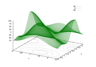
(a) Potential cut at $z=3.264$ $\AA$.

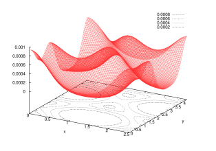
(b) Wave function cut at $z=3.264$ $\AA$.

Figure 1: Numerical solution of the Schrödinger equation for one $D_{2}$ molecule in the C-graphane potential. Only the basic unit cell of the C-graphane is represented.

The $b$ parameters of the corresponding Jastrow functions that appear in (1) were obtained from variational Monte Carlo calculations that included ten deuterium molecules on a C-graphane simulation cell of dimensions 35.47 $\times$ 35.11 Ų. This is a 14$\times$8 supercell of the basic unit defined above. The optimal value is $b$= 3.195 Å, exactly the same number as the one used for graphene in previous calculations [10]. Some other tests made for different deuterium densities left the parameter unchanged.

To simulate solid deuterium phases, we multiplied $\Psi_{L}$ (1) by a product of Gaussian functions whose role is to confine the adsorbate molecules around the crystallographic positions ($x_{I},y_{I}$) of the two dimensional solids we are interested in. We have used the Nosanow-Jastrow model,

$$\Psi_{S}({\bf r}_{1},{\bf r}_{2},\ldots,{\bf r}_{N})=\Psi_{L}\,\prod_{i,I=1}^{N}\exp\{-c[(x_{i}-x_{I})^{2}+(y_{i}-y_{I})^{2}]\}\ ,$$ (2)

where the $c$ parameters are dependent on the particular solid, commensurate or incommensurate. The variationally optimized values for $c$ are given in table 1. For the triangular incommensurate structures, the values listed are the ones for densities $\rho$ = 0.11 Å^-2 and $\rho=$ 0.08 Å^-2. A linear interpolation was used for intermediate adsorbate densities.

Table 1: Optimal values of $c$ parameters in (2).

• Phases	c (Å-2)
  $\sqrt{3}\times\sqrt{3}$	0.53
  $\delta$	0.82
  $\epsilon$	1.02
  4/7	2.38
  7/12	2.74
  Incommensurate solid	3.1 a
  	1.1 b

• ^a For a density of 0.11Å^-2.

• ^b For a density of 0.08Å^-2.

An important issue in the microscopic description of the system is the choice of the empirical potentials between the different species involved that enter in the Hamiltonian. The deuterium-deuterium interaction was the standard of Silvera and Goldman, [17], that depends only on the distance between the center-of-mass of each pair of hydrogen molecules. This is clearly an approximation, since neither the H₂ molecule nor the D₂ one have perfect spherical symmetry. However, the differences between the ideal spheres and the real ellipsoids are small enough to reproduce accurately the experimental bulk phase diagram of H₂ at low pressures [18]. The same can be said of the theoretical description of both H₂ [9] and D₂ [10] adsorbed on graphite.

We expect then, that this intermolecular potential could describe reasonably the phases of D₂ on this novel surface.

The C-D₂ and H-D₂ substrate potentials were assumed to be of Lennard-Jones type. Since the hybridization of the carbon atoms on graphane is $sp^{3}$ instead of the $sp^{2}$ one of graphene and graphite, one cannot use the same parameters as in previous simulations of adsorption on the latter substrates. We resorted then to Ref. [19] were the C-C and H-H Lennard Jones parameters for CH₄ (a compound where the carbon atoms have a $sp^{3}$ hybridization) were given. Then, the Lorentz-Berthelot combination rules were applied, taking the corresponding $\epsilon$ and $\sigma$ D₂-D₂ values from Ref. [20]. The Lennard Jones parameters so obtained are $\epsilon_{C-D_{2}}$ = 43.52 K, $\sigma_{C-D_{2}}$ = 3.2 Å, $\epsilon_{H-D_{2}}$ = 13.42 K, and $\sigma_{H-D_{2}}$ = 2.83 Å. This is our reference set of interaction parameters, that from now on, will be referred to as LJ1. Since we cannot be sure of the accuracy of the approximation used (after all, graphane is not CH₄), we considered another set of Lennard Jones parameters for the H-D₂ interaction (from now on referred to as LJ2). The basic idea is to check if the phase diagram of D₂ on graphane is reasonable robust with respect to variations in the D₂-surface interaction. However, we only changed the H-D₂ parameters with respect to LJ1 because the C atoms are not in direct contact with the D₂ molecules, and therefore their influence on the adsorbed deuterium molecules should be smaller. We derived this LJ2 potential from the same above mentioned parameters for CH₄ (Ref. [19]), but used the D₂-D₂ ones that result from applying backwards the Lorentz-Berthelot rules to the C-H₂ interaction given in Ref. [21] for H₂ adsorbed on graphite. Obviously, the results derived for H₂ are valid for D₂, since the interaction potentials depend on the electronic structure of the atoms or molecules involved, and this is the same for both hydrogen isotopes. Using this last approximation, one gets $\epsilon_{H-D_{2}}=$17.86 K and $\sigma_{H-D_{2}}$ = 2.56 Å for this second interaction. Unfortunately, we cannot choose a potential set as been more accurate than the other, since there are not experimental data on the binding energy of D₂ on graphane to compare to. Our only goal is then to see if both phase diagrams are similar to each other. This would mean that we have a reasonable description of the experimental phases of deuterium on graphane, in the same way that we can describe accurately the behaviour of the same adsorbate on graphite using similar potentials [9, 10].

The primary output of the application of the DMC method is the local energy, $E_{L}$, whose statistical mean for large enough imaginary time corresponds to the ground-state energy of the system. [16] Explicitly,

$$E_{L}=\Psi({\bf r}_{1},{\bf r}_{2},\ldots,{\bf r}_{N})^{-1}H\Psi({\bf r}_{1},{\bf r}_{2},\ldots,{\bf r}_{N})\ ,$$ (3)

where

$$H=-\frac{\hbar^{2}}{2m}\sum_{i=1}^{N}\bm{\nabla}_{i}^{2}+\sum_{1=i<j}^{N}V_{D_{2}-D_{2}}(r_{ij})+\sum_{m,i=1}^{N_{C},N}V_{C-D_{2}}(r_{mi})+\sum_{n,i=1}^{N_{H},N}V_{H-D_{2}}(r_{ni})$$ (4)

is the Hamiltonian of the system. $\Psi$ stands for $\Psi_{L}$ or $\Psi_{S}$ depending on the phase considered. The local energy is our estimator for the ground state energy of a system described by a given trial function. This is equivalent to say that we operate always at T = 0 K, temperature at which the free energy of a system equals its energy. If we compare then different arrangements of particles (described by different trial functions), the one whose energy per particle is minimum will be the ground state of the system as a whole. If we consider now arrangements with higher densities, we will eventually reach other stable phases, whose density limits will be determined via a standard double-tangent Maxwell construction [22].

3 RESULTS

The phase diagram of D₂ on graphane can be derived from the DMC energies reported in figure 2. There, all the symbols correspond to simulation results both for a translational invariant system (liquid, inverted triangles) and to different two-dimensional solids. We plotted the energy per D₂ molecule versus the surface area, which is the inverse of the deuterium surface density. In that way, to perform the necessary double-tangent Maxwell constructions to determine the stability regions of the different phases is straightforward. The solid arrangements considered were the standard triangular incommensurate phase, and the same commensurate structures taken into account in a previous calculation of D₂ on graphene ($\sqrt{3}\times\sqrt{3}$, $\delta$, and $\epsilon$ phases). [10] Those registered phases were taken as such with respect to the projections of the carbon atoms on the $z$ = 0 plane, projections that form a honeycomb lattice. We tried also some structures that were commensurate with respect to the atomic hydrogen triangular lattice, taking as a model the ones proposed for a second layer of ⁴He on graphene, [23] i.e., the $4/7$ and $7/12$ phases. That system could be considered analogous to the one in the present work because a second ⁴He layer rests also on top of a triangular helium substrate. Our present results show that both the 4/7 and 7/12 structures have similar energies per hydrogen molecule than their incommensurate counterparts at the same densities (see figures 2 and 3), so there is no way to know if they are separate phases. It is worth noticing that the graphane unit cell that builds up the entire structure is bigger than that of graphene. This means that the corresponding adsorbate densities are lower than for a similar arrangement in graphene. For instance, a structure equivalent to the $\sqrt{3}\times\sqrt{3}$ solid in C-graphane has a density of 0.0600 Å^-2 instead of the value 0.0636 Å^-2 found in graphene and graphite.

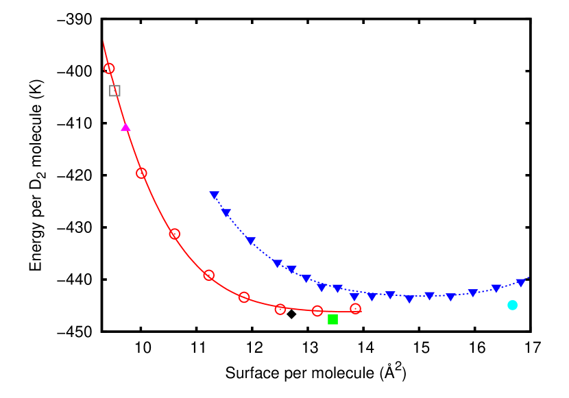
Figure 2: Phase diagram for D₂ on graphane using the set of parameters LJ1. Full circles, $\sqrt{3}\times\sqrt{3}$. Full squares, $\delta$ phase. Solid diamond, $\epsilon$ phase. Full triangle, 4/7 phase; open square, 7/12 commensurate solid. The liquid arrangements are represented by inverted full triangles, while the open circles correspond to the incommensurate triangular solid. The solid and dashed lines are fourth-order polynomial fits to their corresponding data sets. The error bars are of the same size of the symbols and are not displayed for simplicity.

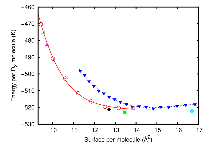
Figure 3: Same as in figure 2, but for the set of Lennard-Jones parameters LJ2

In figure 2, all the calculations were performed using the LJ1 set of Lennard-Jones parameters. To check the influence of the adsorbate-surface interaction in the phase diagram, we used the alternative LJ2 potential. Those results are displayed in figure 3. The obvious conclusion from figure 2 and figure 3 is that, irrespectively of the Lennard-Jones parameters employed, and in the density range represented in both figures, the structure with lowest energy per particle for D₂ on C-graphane is a $\delta$ commensurate solid, lower than the corresponding to a $\sqrt{3}\times\sqrt{3}$ commensurate structure, and lower than for a liquid arrangement. The corresponding energies for each phase are listed in table 2. $E_{0}$ stands for the minimum energy per particle in the liquid phase, obtained from a fourth-order polynomial fit to the energies per particle displayed in figure 2 and figure 3. The binding energy of a single D₂ molecule on top of C-graphane surface is also given. This allows us to say that all the two dimensional adsorbed phases are less stable than their counterparts on graphene. The $\delta$ structure is sketched in figure 4. The big diamond displayed is its unit cell, comprising 31 molecules. Four of these cells can be accommodated in a rectangular simulation cell of dimensions 38.0055 $\times$ 43.8890 Ų. This cell is big enough to prevent any size effects to appear. We did not display the $\sqrt{3}\times\sqrt{3}$ solid since it is a standard well known arrangement (see for instance the same structure on graphite in Ref. [4]). The same can be say of the incommensurate triangular solid (see below).

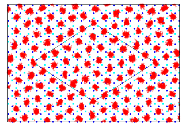
Figure 4: Sketch of the $\delta$ structure. Solid smudges are the result of displaying 300 sets of deuterium coordinates represented as crosses. Solid circles are the projection on the $z=0$ plane of the positions of the carbon atoms bound to the upper H atoms in the C-graphane structure. Solid squares represent the carbon atoms bound to the bottom hydrogens in the skeleton. The big diamond is the unit cell for this arrangement.

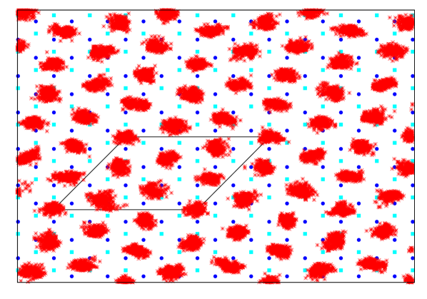
Figure 5: Same as in figure 4 for the $\epsilon$ arrangement. The rhomboid represents the unit cell.

Table 2: Energies in the infinite dilution limit, $E_{\infty d}$. Energies per molecule at the minima of the liquid curves in figure 2 and figure 3, $E_{0}$ . Third, fourth and fifth columns show the adsorption energies of the liquid, $\sqrt{3}\times\sqrt{3}$ and $\delta$ phases respectively with respect the infinite dilution limit. For comparison, the same results for graphene [10] are also included.

	$E_{\infty d}(K)$	$E_{0}(K)$	$\left(E_{0}-E_{\infty d}\right)(K)$	$\left(E_{\sqrt{3}\times\sqrt{3}}-E_{\infty d}\right)(K)$	$\left(E_{\delta}-E_{\infty d}\right)(K)$
LJ1-graphane	-407.6330$\pm$0.0001	-443.3$\pm$0.3	-35.6$\pm$0.3	-37.279$\pm$0.006	-40.01$\pm$0.02
LJ2-graphane	-484.0974$\pm$0.0001	-520.1$\pm$0.3	-36.0$\pm$0.3	-38.121$\pm$0.006	-38.90$\pm$0.02
graphene	-464.87$\pm$0.06	-497.2$\pm$0.9	-32.3$\pm$0.9	-43.66$\pm$0.06	-40.75$\pm$0.07

On increasing the D₂ density, the next stable phase will be the $\epsilon$ registered phase of density 0.0787 Å^-2, and represented by a solid diamond both in figure 2 and figure 3). Its sketch is given in figure 5, that displays its unit cell containing seven molecules. We can accommodate 112 D₂ molecules of this arrangement in a rectangular simulation cell of 40.5392 $\times$ 35.1112 Ų, also big enough to avoid any kind of size effects. A piece of that simulation cell, enough to show the primitive unit, is displayed in figure 5. Since the $\delta$ and $\epsilon$ structures are represented by a single density, the double tangent Maxwell construction between them is simply the line that joints both symbols. In both figures and in table 3, we can see that the $\epsilon$ solid is more stable that an incommensurate arrangement of the same density. This means that upon a density increase, the phase diagram for D₂ on C-graphane would proceed through the sequence $\delta$ $\rightarrow$ $\epsilon$ $\rightarrow$ incommensurate triangular solid. The lowest density of the incommensurate lattice (obtained from a Maxwell construction between the $\epsilon$ and this structure) was 0.084 $\pm$ 0.002 Å^-2 for both series of Lennard-Jones parameters.

Table 3: Energies per molecule and densities of the different phases of D₂ on graphane.

• 		LJ1		LJ2
  Phases	Density ($\AA^{-2}$)	Energy(K)	Energy(K)	Energy(K)	Energy(K)
  Liquid		-443.3$\pm$0.3a		-520.1$\pm$0.3b
  $\sqrt{3}\times\sqrt{3}$	0.0600	-444.912 $\pm$0.006	-440.8$\pm$0.3c	-522.218 $\pm$ 0.006	-518.3$\pm$0.3c
  $\delta$	$0.0743$	-447.64$\pm$ 0.02	-446.0$\pm$0.1d	-523.00 $\pm$0.02	-520.5$\pm$0.3d
  $\epsilon$	$0.0787$	-446.64$\pm$ 0.02	-445.7$\pm$0.1d	-521.29$\pm$ 0.02	-519.6$\pm$0.2d

• ^aAt density 0.067$\pm$0.001 $\AA^{-2}$

• ^bAt density of 0.055$\pm$0.001 $\AA^{-2}$

• ^ccomparison with the liquid phase.

• ^dcomparison with the incommensurate solid.

4 CONCLUSIONS

We calculated the phase diagram of D₂ on C-graphane, a novel substance that has been experimentally realized. Both the structure of the compound and all the interactions between the different parts of the system were taken to be as much realistic as possible. This means that the results of our work could be checked against experimental data in the future. The fact that both the stable phases and their density limits were unchanged by modifications of the surface-deuterium interaction potentials makes us confident in the reliability of the method and in our conclusions. Since we have no experimental data to compare to, we cannot reach any conclusion about the deuterium adsorption energies. In this, we are at disadvantage with the case of graphene, for which we do not have experimental data either, but whose energies could be compared to those of graphite, a close related compound.

Our results also indicate that the ground state of deuterium adsorbed on graphane is the registered phase $\delta$, what makes D₂ on graphane different from H₂ on graphane [12], or from D₂ or any other quantum gas on graphene [8, 9, 10], where the ground states were $\sqrt{3}\times\sqrt{3}$ arrangements. This is also at odds with some recent results for ⁴He on graphane. [11] Those indicate that the ground state of ⁴He on graphane was a liquid, and that a registered phase analogous to the $4/7$ structure was also stable. We did not found that the energy per molecule of that phase were appreciably different than the corresponding to an incommensurate triangular phase of the same density for D₂. In any case, the differences between the phase diagrams on graphene and graphane could make the last one an interesting object of experimental study in the future.

References

References

- [1] S. Iijima, Nature (London) 354, 56 (1991).
- [2] K.S. Novoselov, A.K. Geim, S.V. Morozov, D. Jiang, Y. Zhang, S.V. Dubonos, I.V. Grigorieva, and A.A. Firsov, Science 306, 666 (2004).
- [3] K.S. Novoselov, D. Jiang, F. Schedin, T.J. Booth, V.V. Khotkevich, S.V. Morozov, and A.K. Geim, PNAS 102, 10451 (2005).
- [4] L.W. Bruch M. W. Cole, and E. Zaremba, Physical adsorption: forces and phenomena, Oxford University Press, Oxford (1997).
- [5] J.O. Sofo, A.S. Chaudhary, and G.D. Barber, Phys. Rev. B 75, 153401 (2007).
- [6] E. Caldeano, P.L. Palla, S. Giordano, and L. Colombo, Phys. Rev. B 82, 235414 (2010).
- [7] D.C. Elias, R.R. Nair, T.M.G. Mohiuddin, S.V. Morozov, P. Blake, M.P. Halsall, A.C. Ferrari, D.W. Boukhvalov, M.I. Katsnelson, A.K. Geim, and K.S. Novoselov, Science 323, 610 (2009).
- [8] M.C. Gordillo and J. Boronat, Phys. Rev. Lett. 102, 085303 (2009).
- [9] M.C. Gordillo and J. Boronat, Phys. Rev. B 81, 155435 (2010).
- [10] C. Carbonell-Coronado and M.C. Gordillo, Phys. Rev. B 85, 155427 (2012).
- [11] N. Nava, O.E. Galli, M.W. Cole, and L. Reatto, Phys. Rev. B 86, 174509 (2012).
- [12] C. Carbonell-Coronado, F. De Soto, C. Cazorla, J. Boronat, and M.C. Gordillo, J. Low Temp. Phys. 171, 619 (2013).
- [13] H. Freimuth and H. Wiechert, Surf. Sci. 162, 432 (1985).
- [14] H. Freimuth and H. Wiechert, Surf. Sci. 189/190, 548 (1987).
- [15] H. Freimuth, H. Wiechert, H.P. Schildberg, and H.J. Lauter, Phys. Rev. B. 42, 587 (1990).
- [16] J. Boronat and J. Casulleras, Phys. Rev. B 49, 8920 (1994).
- [17] I. F. Silvera and V. V. Goldman, J. Chem. Phys. 69, 4209 (1978).
- [18] T. Omiyinka and M. Boninsegni, Phys. Rev B 88 024212 (2013).
- [19] J.M. Phillips and M.D. Hammerbacher, Phys. Rev. B. 29, 5859 (1984).
- [20] G. Stan, M.J. Bojan, S. Curtarolo, S. Gatica, and M.W. Cole, Phys. Rev. B 62, 2173 (2000).
- [21] G. Stan and M.W. Cole, J. Low Temp. Phys. 110, 539 (1998).
- [22] D. Chandler, Introduction to modern statistical mechanics, Oxford University Press, Oxford (1987).
- [23] M.C. Gordillo and J. Boronat, Phys. Rev. B 85, 195457 (2012).