Bayesian variable selection for latent class analysis using a collapsed Gibbs sampler

Abstract

Latent class analysis is used to perform model based clustering for multivariate categorical responses. Selection of the variables most relevant for clustering is an important task which can affect the quality of clustering considerably. This work considers a Bayesian approach for selecting the number of clusters and the best clustering variables. The main idea is to reformulate the problem of group and variable selection as a probabilistically driven search over a large discrete space using Markov chain Monte Carlo (MCMC) methods. Both selection tasks are carried out simultaneously using an MCMC approach based on a collapsed Gibbs sampling method, whereby several model parameters are integrated from the model, substantially improving computational performance. Post-hoc procedures for parameter and uncertainty estimation are outlined. The approach is tested on simulated and real data.

1 Introduction

Latent class analysis (LCA) models (Goodman, 1974) are used to discover affinities and groupings in multivariate categorical data. An example of data for which a LCA model may be appropriate would be records for $N$ items on $M$ different variables where each of the variables observed is categorical, more precisely, binary or nominal. There may be a varying number of categories over the $M$ different variables. In using a LCA model one expects the items to segment into groups within which items are similar in nature. These groupings are captured by allowing the variables’ multinomial probabilities to vary by group.

LCA models have been widely studied and applied (Aitkin et al, 1981; Garrett and Zeger, 2000; Walsh, 2006). They can be viewed as a special case of model-based clustering (McLachlan and Peel, 2002; Fraley and Raftery, 2007), in which each item is assumed to arise from one of a number of groups, each group having its own data probability distribution. As with other applications of clustering, two of the main difficulties when formulating a LCA model are identifying a suitable number of different groups or clusters in the data, and choosing the variables which are most informative for groupings in the data.

Dean and Raftery (2010) have demonstrated that both of these aspects of model selection can have a considerable effect on the resulting clustering of the data, and that these questions are important in the formulation and application of LCA models. Their approach learns from the data using a headlong search algorithm to choose the optimal clustering variables and number of groups, with steps in the algorithm determined using the Bayesian Information criterion (BIC) (Schwarz, 1978; Kass and Raftery, 1995).

In this paper, a Bayesian approach for the analysis of LCA models is proposed. It is shown how simple marginalization of the parameters in a LCA model leads to a form of the model for which Markov chain Monte Carlo (MCMC) sampling algorithms can be used to quantify precisely the uncertainty in the number of groups in the data, as well as which variables give the best clustering. This is similar to work carried out by Nobile and Fearnside (2007) in the analysis of Gaussian finite mixtures, Wyse and Friel (2012) in a block clustering application, McDaid et al (2013) in the clustering of social network data, and Tadesse et al (2005) in the context of clustering variable selection for Gaussian distributed data.

The advantage of such an approach is that it allows us to see which of the variables hold information on the clustering of the data. This gives more information than would be available from the headlong search algorithm in Dean and Raftery (2010) which gives a point estimate of the variables which optimally determine the clustering, but does not include any quantification of the uncertainty around these particular choices.

The rest of this paper is organised as follows. Section 2 outlines model specification for LCA in detail and gives a brief overview of other approaches for analysis that have been proposed in the literature. The five datasets which the method is applied to are then introduced and described. Section 3 presents the adopted marginalization approach and gives details of the MCMC algorithm used to estimate the models. Section 4 discusses estimation of posterior quantities from the model, including parameter estimation, how model comparison may be performed by computing approximate posterior model probabilities, as well as a description of how label switching is accounted for. Section 5 applies the sampling algorithm to simulated and real data, concluding with a discussion in Section 6.

2 The classic LCA model

Denote the data by an $N\times M$ matrix $\mathbf{X}$ where each row is a record of responses for $M$ categorical variables for one item. Row $n$ of $\mathbf{X}$ is $\mathbf{X}_{n}=(X_{n1},X_{n2},\dots,X_{nM})$. The entry $X_{nm}$ takes a value from one of the categories $\{1,2,\dots,C_{m}\}$ for variable $m$. The LCA model assumes that the $\mathbf{X}_{n}$ arise independently from a finite mixture model with $G$ components or classes,

$$p(\mathbf{X}_{n}|\mbox{\boldmath{$\tau$}},\mbox{\boldmath{$\theta$}},G)=\sum_{g=1}^{G}\tau_{g}p(\mathbf{X}_{n}|\mbox{\boldmath{$\theta$}}_{g}).$$

The $\tau_{g}$ are mixture weights, with $\sum_{g=1}^{G}\tau_{g}=1$ and $\tau_{g}>0$, for all $g$. Each component has its own set of parameters $\mbox{\boldmath{$\theta$}}_{g}$ which embody the differences between groups; this holds the multinomial probabilities for all variables for class $g$. The parameter $\theta_{gmc}$ corresponds to the probability that an item takes category $c$ for variable $m$ within class $g$. For the component data likelihood, a local independence assumption is made. This assumes that, conditional on an observation’s group membership, all variables are independent of each other, so that

$$p(\mathbf{X}_{n}|\mbox{\boldmath{$\theta$}}_{g})=\prod_{m=1}^{M}\prod_{c=1}^{C_{m}}\theta_{gmc}^{\mathrm{I}(X_{nm}=c)},$$

where

$${\mathrm{I}(X_{nm}=c)}=\left\{\begin{array}[]{ll}1&\mbox{if $X_{nm}=c$}\\ 0&\mbox{otherwise.}\end{array}\right.$$

It is convenient to work with the completed data, that is, data augmented with class labels for each item. Denote these by $\mathbf{Z}$, where

$$Z_{ng}=\left\{\begin{array}[]{ll}1&\mbox{if observation $n$ belongs to group $g$}\\ 0&\mbox{otherwise.}\end{array}\right.$$

The completed data likelihood for an observation may then be written

$$p(\mathbf{X}_{n},\mathbf{Z}_{n}|\mbox{\boldmath{$\theta$}},\mbox{\boldmath{$\tau$}},G)=\prod_{g=1}^{G}\left\{\tau_{g}\prod_{m=1}^{M}\prod_{c=1}^{C_{m}}\theta_{gmc}^{\mathrm{I}(X_{nm}=c)}\right\}^{Z_{ng}}.$$

2.1 Approaches for analysis

When the number of groups and variables is assumed fixed, several techniques for performing LCA are available. When attempting to identify the number of groups in the data, models are fitted over a range of groups, with the best fit often determined with the use of an information criterion.

In a frequentist paradigm, an expectation-maximisation (EM) algorithm (Dempster et al, 1977) can be employed. The BIC or Akaike’s information criterion (AIC) (Akaike, 1973) can then be used to identify an optimal model. Goodness-of-fit statistics such as the likelihood ratio test (Goodman, 1974) can also be employed, but may prove difficult to apply to sparse data with a large number of variables (Aitkin et al, 1981).

In a Bayesian paradigm, for a fixed model, a Gibbs sampling (Geman and Geman, 1984; Garrett and Zeger, 2000) technique can be used. When several competing models are possible, additional inference methods must also be used to take account of this additional model uncertainty. Garrett and Zeger (2000) propose graphical tools to aid model selection, and detect weak identifiability. If the difference between these distributions is judged to be small, this then suggests that too large a number of groups has been fitted to the data. Frühwirth-Schnatter (2006, Chapter 5) contains an excellent overview of many of the following methods, which take a more principled approach.

Monte Carlo based integration of the marginal likelihood can be used to inform model selection (Bensmail et al, 1997). Frühwirth-Schnatter (2004) demonstrates this approach for mixture models using importance sampling (Geweke, 1989) or the more general bridge sampling methods (Meng and Wong, 1996), while Chopin and Robert (2010) use a nested sampling approach. Using a harmonic mean estimator (Newton and Raftery, 1994), Raftery et al (2007), propose the information criteria AIC or BIC Monte Carlo (AICM or BICM). An alternative information criterion, the deviance information criterion (Spiegelhalter et al, 2002), has also been proposed, although this approach has been criticized for its somewhat opaque specification; this can lead to different results depending on its interpretation when used in a mixture model setting (Celeux et al, 2006).

Another approach for Bayesian model selection is to use trans-dimensional MCMC techniques such as reversible jump MCMC (RJMCMC) methods (Green, 1995) or Markov birth-death processes (Stephens, 2000a; Cappé et al, 2003). While RJMCMC has previously been extended to univariate and multivariate finite Gaussian mixture models(Richardson and Green, 1997; Dellaportas and Papageorgiou, 2006), only recently has it been applied to latent class analysis (Pan and Huang, 2013; Pandolfi et al, 2014); however, these approaches do not consider variable selection. Tadesse et al (2005) make use of the RJMCMC method to also perform variable selection, with some parameters integrated from the model. We base our approach on an alternative method, a fully collapsed sampler first proposed by Nobile and Fearnside (2007).

Technical issues can also occur when fitting LCA, such as underestimation of standard errors when using the EM algorithm (Bartholomew and Knott, 1999; Walsh, 2006), and label-switching for Gibbs sampling (Marin et al, 2005). The latter issues, and the methods used to avoid them, are discussed in Section 4.

2.2 Datasets to be analysed

We provide a description of the five datasets which are analysed in Section 5. The first examples are simulated data, while two of the three real datasets have been previously analysed using the LCA methods described in Section 2.1. The last dataset we examine has not been analysed using LCA before now. We examine both binary and non-binary examples. Four of our examples are binary, so that $C_{m}=2,\mbox{ and }X_{nm}\in\{1,2\}$ for all possible values of $n$ and $m$. One of the examples is non-binary, and has $C_{m}$ varying from 2 up to 5 over the different variables.

Dean and Raftery simulated datasets

We first test our approach on simulated datasets as specified by Dean and Raftery (2010). The first is a binary two class model of $N=500$ observations with 4 informative variables (1-4) and 9 noise variables (5-13), with class weights set to $\tau_{1}=0.6$ and $\tau_{2}=0.4$. The specified parameter values for $\boldsymbol{\theta}$ are given in Table 1.

The second simulated dataset is a non-binary three class model with $N=1000$ observations. Again there are 4 informative variables (1-4) and 6 noise variables (5-10). The class weights are $\tau_{1}=0.3$, $\tau_{2}=0.4$ and $\tau_{3}=0.3$. The values for $\boldsymbol{\theta}$ for the informative variables are given in Table 2 and those for the non-informative variables are given in Table 3.

Table 1: Multinomial probabilities $\boldsymbol{\theta}$ in the Dean and Raftery simulated dataset.

Variable	Class 1	Class 2
1	0.6	0.2
2	0.8	0.5
3	0.7	0.4
4	0.6	0.9
5	0.5	0.5
6	0.4	0.4
7	0.3	0.3
8	0.2	0.2
9	0.9	0.9
10	0.6	0.6
11	0.7	0.7
12	0.8	0.8
13	0.1	0.1

Table 2: Specified parameter values for $\boldsymbol{\theta}$ in the non-binary Dean and Raftery simulated dataset for the discriminating variables.

Variable	Category	Class 1	Class 2	Class 3
1	1	0.1	0.3	0.6
	2	0.1	0.5	0.2
	3	0.8	0.2	0.2
2	1	0.5	0.1	0.7
	2	0.5	0.9	0.3
3	1	0.2	0.7	0.2
	2	0.2	0.1	0.6
	3	0.3	0.1	0.1
	4	0.3	0.1	0.1
4	1	0.1	0.6	0.4
	2	0.5	0.1	0.4
	3	0.4	0.3	0.2

Table 3: Specified parameter values for $\boldsymbol{\theta}$ in the non-binary Dean and Raftery simulated dataset for the non-discriminating variables.

Variable	Category	All classes
5	1	0.4
	2	0.5
	3	0.1
6	1	0.2
	2	0.4
	3	0.1
	4	0.3
7	1	0.2
	2	0.3
	3	0.3
	4	0.1
	5	0.1
8	1	0.2
	2	0.8
9	1	0.7
	2	0.1
	3	0.2
10	1	0.1
	2	0.2
	3	0.1
	4	0.6

Alzheimer dataset

This dataset of patient symptoms was recorded in the Mercer Institute of St. James’ Hospital in Dublin, Ireland (Moran et al, 2004; Walsh, 2006). The data consist of a record of the presence or absence of $M=6$ symptoms displayed by $N=240$ patients diagnosed with early onset Alzheimer’s disease, and are available in the R(R Core Team, 2013) package BayesLCA(White and Murphy, 2013). Previous studies had difficulty in determining whether two or three groups are more suitable for the data, where fitting a three group model also created difficulties when performing inference (Walsh, 2006).

Teaching styles dataset

This dataset was collected in an attempt to ascertain the different types of teaching style being employed in schools in the United Kingdom in the mid 1970s, and was discussed at length by Aitkin et al (1981) after an initial analysis by Bennet (1976). The dataset records which of $M=39$ teaching methods are employed by the $N=467$ schools. Computational limitations at the time meant that only a two or three group clustering of the data were seriously considered, with dimension reduction in a previous study performed using principal component analysis. Further, use of information based criteria such as the BIC had not been developed at that time, so that no automatic comparison of the clusterings could be made, with a decision on the optimal clustering being based on careful consideration of the different properties of the clusterings.

Physiotherapy dataset

We also apply our methods to a physiotherapy dataset based on a survey recently conducted by Keith Smart in St. Vincent’s University Hospital, Dublin (Smart et al, 2011). The aim of this study was to identify which symptoms distinguish between three types of back pain which patients suffer from. The dataset consists of $N=425$ observations and $M=36$ variables. While the different types of back pain were considered reasonably distinct, different subgroups of pain sufferers within these pain classes are also possible, which motivates an examination of the data in an unsupervised setting.

3 Bayesian latent class model and marginalization approach

In this section, a variable inclusion indicator variable is introduced, and a fully Bayesian specification for LCA is provided. A collapsed sampling scheme for inference is then described.

3.1 Clustering variable selection

The marginalization approach addresses exploring uncertainty in variable selection for clustering the items as well as uncertainty in the number of classes, $G$. To this end, let $\boldsymbol{\nu}_{\mathrm{cl}}$ be a vector containing the indexes of the set of variables used for clustering the data and $\boldsymbol{\nu}_{\mathrm{n}}$ contain the remaining indexes of variables not used for clustering the data. To make this clearer, we formulate the data model by using two parts. For brevity, we use $\boldsymbol{\nu}$ to denote $(\boldsymbol{\nu}_{\mathrm{cl}},\boldsymbol{\nu}_{\mathrm{n}})$. The variables in $\boldsymbol{\nu}_{\mathrm{cl}}$ follow an LCA model with $G$ classes. This gives the likelihood

$$p_{\mathrm{cl}}(\mathbf{X},\mathbf{Z}|\mbox{\boldmath{$\theta$}},\mbox{\boldmath{$\nu$}},\mbox{\boldmath{$\tau$}},G) = \prod^{N}_{n=1}\prod_{g=1}^{G}\left\{\tau_{g}\prod_{m\in\nu_{\mathrm{cl}}}\right.$$

$$\times \left.\prod_{c=1}^{C_{m}}\theta_{gmc}^{\mathrm{I}(X_{nm}=c)}\right\}^{Z_{ng}}.$$

The second part of the model concerns $\boldsymbol{\nu}_{\mathrm{n}}$. The variables in this index vector can still be seen to follow an LCA model, independent of that above. However, this time, the LCA model has just one class. This is since these variables do not hold information on the clustering. This gives the likelihood

$$p_{\mathrm{n}}(\mathbf{X}|\mbox{\boldmath{$\rho$}},\mbox{\boldmath{$\nu$}})=\prod_{n=1}^{N}\prod_{m\in\nu_{\mathrm{n}}}\prod_{c=1}^{C_{m}}\rho_{mc}^{\mathrm{I}(X_{nm}=c)},$$

where $\rho_{mc}$ is the probability of variable $m$ having category $c$.

3.2 Prior assumptions and joint posteriors

Prior assumptions for all sets of multinomial probabilities as well as the component weights $\tau$ are independent Dirichlet distributions. For example, for the clustering variables $m\in\boldsymbol{\nu}_{\mathrm{cl}}$

$$p(\mbox{\boldmath{$\theta$}}_{gm}|\beta)=\frac{\Gamma\left(C_{m}\beta\right)}{\Gamma\left(\beta\right)^{C_{m}}}\prod_{c=1}^{C_{m}}\theta_{gmc}^{\beta-1}.$$

The hyperparameters $\beta$ are chosen to be 1 for all $g,m$ combinations. A Dirichlet prior is also assumed for those variables $m\in\nu_{\mathrm{n}}$, where the hyperparameters $\beta$ are again chosen to be 1 in all cases:

$$p(\mbox{\boldmath{$\rho$}}_{m}|\beta)=\frac{\Gamma\left(C_{m}\beta\right)}{\Gamma\left(\beta\right)^{C_{m}}}\prod_{c=1}^{C_{m}}\rho_{mc}^{\beta-1}.$$

For the component weights the prior assumed is

$$p(\mbox{\boldmath{$\tau$}}|\alpha,G)=\frac{\Gamma\left(G\alpha\right)}{\Gamma\left(\alpha\right)^{G}}\prod_{g=1}^{G}\tau_{g}^{\alpha-1}$$

where $\alpha$ is taken to be 0.5, for all possible values of $g$; this is the marginal Jeffreys for the multinomial model, and is partly chosen to discourage overfitting (Rousseau and Mengersen, 2011).

It is assumed that the prior probability of any variable being a clustering variable is $\pi$, giving a joint prior for $\nu$ of

$$p(\mbox{\boldmath{$\nu$}}|{\pi})=\prod_{m\in\nu_{\mathrm{cl}}}\pi\prod_{m\in\nu_{\mathrm{n}}}(1-\pi).$$

This prior is independent of the priors on $\mbox{\boldmath{$\theta$}},\mbox{\boldmath{$\rho$}}$ and $\boldsymbol{\tau}$.  Ley and Steel (2009) give a detailed discussion of this prior on variable inclusion. They conclude that further assuming a $\mbox{Beta}(a_{0},b_{0})$ hyperprior on $\pi$ can be much more sensible than using a fixed value of $\pi$. We investigate the use of such a hyperprior in analyzing the Alzheimer data in Section 5.2. When a hyperprior is not used, a value of $\pi=0.5$ is assumed for the applications in this paper.

The complete data likelihood for all variables is

$$p_{\mathrm{full}}(\mathbf{X},\mathbf{Z}|\mbox{\boldmath{$\theta$}},\mbox{\boldmath{$\rho$}},\mbox{\boldmath{$\nu$}},\mbox{\boldmath{$\tau$}},G)=p_{\mathrm{cl}}(\mathbf{X},\mathbf{Z}|\mbox{\boldmath{$\theta$}},\mbox{\boldmath{$\nu$}},\mbox{\boldmath{$\tau$}},G)p_{\mathrm{n}}(\mathbf{X}|\mbox{\boldmath{$\rho$}},\mbox{\boldmath{$\nu$}})$$

and the joint posterior for the unknowns (except the number of classes) is

$$p(\mathbf{Z},\mbox{\boldmath{$\theta$}},\mbox{\boldmath{$\rho$}},\mbox{\boldmath{$\nu$}},\mbox{\boldmath{$\tau$}}|\mathbf{X},G,\alpha,\pi,\beta) \propto p_{\mathrm{full}}(\mathbf{X},\mathbf{Z}|\mbox{\boldmath{$\theta$}},\mbox{\boldmath{$\rho$}},\mbox{\boldmath{$\nu$}},\mbox{\boldmath{$\tau$}},G)$$

$$\times p(\mbox{\boldmath{$\tau$}}|\alpha,G)p(\mbox{\boldmath{$\nu$}}|\pi)$$

$$\times \prod_{m\in\nu_{\mathrm{n}}}p(\mbox{\boldmath{$\rho$}}_{m}|\beta)$$

$$\times \prod_{g=1}^{G}\prod_{m\in\nu_{\mathrm{cl}}}p(\mbox{\boldmath{$\theta$}}_{gm}|\beta).$$

Under the model being considered there is also uncertainty in the number of classes. This is accounted for by taking a prior on $G$, which we assume to be $\mathrm{Poisson}(1)$, truncated to $\{1,\dots,G_{\mathrm{max}}\}$, with $G_{\mathrm{max}}$ the maximum number of classes considered feasible. We choose this prior for $G$ following its justification by Nobile (2005) in the analysis of Bayesian finite mixtures. The full posterior is then

$$p(G,\mathbf{Z},\mbox{\boldmath{$\theta$}},\mbox{\boldmath{$\rho$}},\mbox{\boldmath{$\nu$}},\mbox{\boldmath{$\tau$}}|\mathbf{X},\alpha,\pi,\beta)$$

$$\qquad\propto p(\mathbf{Z},\mbox{\boldmath{$\theta$}},\mbox{\boldmath{$\rho$}},\mbox{\boldmath{$\nu$}},\mbox{\boldmath{$\tau$}}|\mathbf{X},G,\alpha,\pi,\beta)p(G).$$

Note that this derivation of the posterior assumes that $\pi$ is a fixed value. If we include the hyperprior on $\pi$ discussed above, the right hand side of this proportionality relation has an extra multiplicative term $p(\pi)=\mbox{be}(\pi;a_{0},b_{0})$, where $\mbox{be}(\cdot;a_{0},b_{0})$ is the beta density with shape parameters $a_{0}$ and $b_{0}$.

3.3 Marginalization approach

The marginalization approach proceeds by observing that all of the multinomial probabilities, as well as the component weights can be marginalized analytically out of the model by using the normalizing constant of the Dirichlet distribution. This leaves a joint distribution for $G$, $\nu$ and $\mathbf{Z}$:

$$p(G,\mathbf{Z},\mbox{\boldmath{$\nu$}}|\mathbf{X},\alpha,\pi,\beta)$$

$$\propto p(G)\int p(\mathbf{Z},\mbox{\boldmath{$\theta$}},\mbox{\boldmath{$\rho$}},\mbox{\boldmath{$\nu$}},\mbox{\boldmath{$\tau$}}|\mathbf{X},G,\alpha,\pi,\beta)\,d\mbox{\boldmath{$\theta$}}\,d\mbox{\boldmath{$\rho$}}\,d\mbox{\boldmath{$\tau$}}.$$

Carrying out this marginalization gives

$$p(G,\mathbf{Z},\mbox{\boldmath{$\nu$}}|\mathbf{X},\alpha,\pi,\beta)$$ (1)

$$\propto p(G)p(\mbox{\boldmath{$\nu$}}|\pi)\frac{\Gamma\left(G\alpha\right)}{\Gamma\left(\alpha\right)^{G}}\frac{\prod_{g=1}^{G}\Gamma\left(N_{g}+\alpha\right)}{\Gamma\left(N+G\alpha\right)}$$

$$\times \prod_{m\in\nu_{\mathrm{n}}}\frac{\Gamma\left(C_{m}\beta\right)}{\Gamma\left(\beta\right)^{C_{m}}}\frac{\prod_{c=1}^{C_{m}}\Gamma\left(N_{mc}+\beta\right)}{\Gamma\left(N+C_{m}\beta\right)}$$

$$\times \prod_{g=1}^{G}\prod_{m\in\nu_{\mathrm{cl}}}\frac{\Gamma\left(C_{m}\beta\right)}{\Gamma\left(\beta\right)^{C_{m}}}\frac{\prod_{c=1}^{C_{m}}\Gamma\left(N_{gmc}+\beta\right)}{\Gamma\left(N_{g}+C_{m}\beta\right)}$$

where $N_{g}$ is the number of observations clustered to group $g$, $N_{mc}$ is the number of times variable $m$ takes category $c$, and $N_{gmc}$ is the number of items in group $g$ that have category $c$ for variable $m$. Of note here is that this posterior makes sampling the number of groups $G$ and the clustering variables $\boldsymbol{\nu}_{\mathrm{cl}}$ possible using standard MCMC techniques as outlined in the following section.

3.4 Sampling algorithm

The sampling algorithm comprises three main operations. The first samples the class membership of observations, the second samples the number of classes and the third step samples the variables useful for clustering.

3.4.1 Class memberships

Class memberships are sampled using a Gibbs sampling step which exploits the full conditional distribution of the class label for observation $n$, $n=1,\dots,N$. Given the current configuration of labels, groups and clustering variables, and supposing that the current $Z_{ng}=1$, we can find the full conditional probability of item $n$ belonging to any class $h\neq g$, by taking it out of class $g$ and putting in this class in (1). The full conditional of remaining in class $g$ is just (1). The values for $h\neq g$ can be normalized by the case where the class remains the same, so that up to a normalizing constant, the full conditional distribution of $\mathbf{Z}_{n}$ is found by:

1. evaluating Equation (1) $G$ times, at the current values of $\{G,\mathbf{Z}\backslash\mathbf{Z}_{n},\nu\}$;

2. setting $Z_{ng}$ to be proportional to its corresponding value, for $g=1\ldots,G$;

3. normalizing the resulting values, so that
   $\sum^{G}_{g=1}Z_{ng}=1.$

Memberships are updated for each observation at each iteration. If we let $C=\sum_{m=1}^{M}C_{m}$, we can see by inspection from this, that the computational effort required to sample the class memberships in one sweep of the algorithm is in the worst case $O(2NMCG)$. There are various scenarios when this can become prohibitive for long runs of the sampler. For example, we may always expect $C$ to not have too large a magnitude, as possibly with $G$ in some cases. If we have reason to believe only a fraction of the $M$ possible variables are relevant for clustering, the main cost comes from the number of samples $N$.

3.4.2 Number of classes

The number of classes may be sampled using the approach introduced by Nobile and Fearnside (2007) for Gaussian mixtures. We outline this approach here. Given that there are currently $G$ components, two Metroplis-Hastings moves may be proposed: either the observations assigned to a component are randomly divided into two groups, so that a new component is “ejected” from an existing one, and the number of groups is increased to $G+1$, or the observations in two distinct groups are merged together, so that a component is “absorbed”, and the number of groups decreases to $G-1$.

A component is added or removed with probability $p_{G}=0.5$ or $1-p_{G}=0.5$, except at the endpoints $G\in\{1,G_{\max}\},$ where they are modified appropriately. A component $k$ is chosen at random to “eject” a new component from. To eject the new component, a draw $u\sim\mathrm{Beta}(a,a)$ is made, and each element of the ejecting component $k$ is assigned to the new component $G+1$ with probability $u$, otherwise it remains in $k$. The choice of shape parameter $a$ can have a strong effect on sampler performance, and is most effective when close to empty components are proposed often. This choice is determined by the size of the ejecting component, and a suitable value may be obtained by, for example, numerical programming. We refer to Appendix A3 in Nobile and Fearnside (2007) for further details.

If the proposed components’ quantities are denoted by a $\tilde{\cdot}$, then the acceptance probability of an eject is $\min(1,A)$ where

$$A = \frac{p(G+1,\tilde{\mathbf{Z}},\mbox{\boldmath{$\nu$}}|\mathbf{X},\alpha,\pi,\beta)}{p(G,\mathbf{Z},\mbox{\boldmath{$\nu$}}|\mathbf{X},\alpha,\pi,\beta)}\times\frac{1-p_{G+1}}{p_{G}}$$

$$\times \frac{\Gamma\left(a\right)^{2}}{\Gamma\left(2a\right)}\times\frac{\Gamma\left(2a+N_{k}\right)}{\Gamma(a+\tilde{N}_{k})\Gamma(a+\tilde{N}_{G+1})}.$$

If the move is accepted, an additional label swap between the ejected component and another of the components selected at random is carried out. This is to improve the mixing properties of the sampler. For the reverse absorption move, one chooses two components $k$ and $k^{\prime}$ at random, and places all items from $k$ into $k^{\prime}$, computing the acceptance probability as $\min(1,A^{-1})$. If accepted, the number of components decreases from $G+1$ to $G$.

3.4.3 Clustering variables

To sample the clustering variables an index $j$ is chosen randomly from $\{1,\dots,M\}$. If $j\in\boldsymbol{\nu}_{\mathrm{n}}$ it is proposed to move it to $\boldsymbol{\nu}_{\mathrm{cl}}$. Alternatively, if $j\in\boldsymbol{\nu}_{\mathrm{cl}}$, it is proposed to move it to $\boldsymbol{\nu}_{\mathrm{n}}$.

If the chosen $j\in\boldsymbol{\nu}_{\mathrm{n}}$, the acceptance probability of the proposal to move it to $\boldsymbol{\nu}_{\mathrm{cl}}$ is $\min(1,R)$ with

$$R = \frac{p(G,\mathbf{Z},\tilde{\mbox{\boldmath{$\nu$}}}|\mathbf{X},\alpha,\pi,\beta)}{p(G,\mathbf{Z},\mbox{\boldmath{$\nu$}}|\mathbf{X},\alpha,\pi,\beta)}$$

$$= \left(\frac{\Gamma\left(C_{j}\beta\right)}{\Gamma\left(\beta\right)^{C_{j}}}\right)^{G-1}\prod^{G}_{g=1}\frac{\prod_{c=1}^{C_{j}}\Gamma(N_{gjc}+\beta)}{\Gamma(N_{g}+C_{m}\beta)}$$

$$\times \left({\frac{\prod_{c=1}^{C_{j}}\Gamma(N_{jc}+\beta)}{\Gamma(N+C_{j}\beta)}}\right)^{-1}\times\left(\frac{\pi}{1-\pi}\right).$$

In this expression $\tilde{\mbox{\boldmath{$\nu$}}}$ is the proposed new allocation of clustering and non-discriminating variables. A similar calculation can be carried out to compute the acceptance probability when the chosen $j\in\boldsymbol{\nu}_{\mathrm{cl}}$.

3.4.4 Sampling $\pi$ with a $\mathrm{Beta}(a_{0},b_{0})$ hyperprior

Taking a $\mathrm{Beta}(a_{0},b_{0})$ hyperprior on $\pi$ as in Ley and Steel (2009), it can be shown that the full conditional of $\pi$ given everything else is $\mathrm{Beta}(|\boldsymbol{\nu}_{\mathrm{cl}}|+a_{0},|\boldsymbol{\nu}_{\mathrm{n}}|+b_{0})$, where $|\mathbf{e}|$ means the number of elements in $\mathbf{e}$. This can be sampled in each sweep using a draw from the beta distribution.

3.4.5 Sampling scheme summary

Each sweep of the algorithm thus takes the following three steps:

1. Update the class membership of observations using a Gibbs sampling step.

2. Propose to add a component with probability $p_{G}$, otherwise propose to absorb (remove) a component.

3. Choose one variable at random. If it is not included to cluster variables, propose to do so. If currently included as a clustering variable, propose to exclude it.

The iterations used for posterior inference are taken after an initial burn-in phase. In addition to the moves above, if one has assumed a hyperprior on $\pi$, a “(d)” step involves sampling from the full conditional in Section 3.4.4. In the applications described in Section 5, diagnostic tools in the R package coda (Plummer et al, 2006) were applied to the log posterior to help determine whether a sufficient number of samples have been run for burn-in to occur, and whether thinning of the resulting samples is required. Visually, trace plots of the log posterior, number of groups and number of variables included can also be used to assess the effectiveness of the sampler.

4 Post-hoc procedures for inference

The MCMC output from running the algorithm described in Section 3.4 can be post-processed in order to perform inference on the clustering of observations, as well as item probability and weight parameter estimation. The first step is to correct the output samples of class labels for label switching. How this is done is outlined in the following. Note that no label switching is required in order to evaluate the number of groups which underly the data, or which variables are useful for clustering. After this, other post-hoc procedures for inference are discussed.

4.1 Label switching

Label switching can occur in the algorithm of Section 3.4. The reason is that

$$p(G,\mathbf{Z},\mbox{\boldmath{$\nu$}}|\mathbf{X},\alpha,\pi,\beta)=p(G,\mathbf{Z}_{\cdot\delta},\mbox{\boldmath{$\nu$}}|\mathbf{X},\alpha,\pi,\beta)$$

where $\mathbf{Z}_{\cdot\delta}$ denotes the indicator matrix obtained by applying any permutation $\delta$ of $1,\dots,G$ to the columns in $\mathbf{Z}$. This invariance to permutations of the labels makes posterior inference of the clusterings fruitless unless some post-processing procedure is employed to try to “undo” the label switching first (Stephens, 2000b; Celeux et al, 2000; Marin et al, 2005). Here, the procedure used is the same as that proposed by Nobile and Fearnside (2007) and discussed in detail in Wyse and Friel (2012). We provide a brief outline in the following.

The method re-labels samples by minimising a cost function of the group membership vectors $\mathbf{Z}$. Let $\mathbf{Z}^{(T)}$ denote the value of the group membership indicator matrix $\mathbf{Z}$ stored at iteration $T$ during the sample run. Then a $G\times G$ cost matrix $\mathbf{C}$ can be created with entries

$$C_{gh}=\sum^{T-1}_{t=1}\sum^{N}_{n=1}(1-Z^{(t)}_{ng}){Z}^{(T)}_{nh}.$$

A cost function for $\mathbf{C}$ can then be constructed which is minimised by the permutation $\delta$ of $\mathbf{Z}^{(T)}_{n}$, $n=1,\ldots,N,$ which minimises the trace of $\mathbf{C}$. This is found using the square assignment algorithm of Carpaneto and Toth (1980).

4.2 Post-hoc parameter estimation

Although we integrate out the mixture weight and item probability parameters $\tau$ and $\theta$ from the model, it is still possible to estimate a posteriori summaries of the parameters. Here we demonstrate how it is possible to obtain parameter expectation and variance estimates, conditional on a given number of groups, from a post-hoc calculation, by making use of the following formulae:

$${\mathbb{E}}[A] = {\mathbb{E}}[{\mathbb{E}}[A|B]]$$

$${\mathbb{V}}\mbox{ar}[A] = {\mathbb{E}}[{\mathbb{V}}\mbox{ar}[A|B]]+{\mathbb{V}}\mbox{ar}[{\mathbb{E}}[A|B]],$$

for any random variables $A$ and $B$. Clearly, in providing these posterior estimates, we condition on a given set of variables in the model for all iterations. These calculations can thus be performed using an auxiliary run of the sampler which keeps only the clustering variables in the model (i.e. no variable search).

Define the following summary statistics, for $t\in 1,\ldots,T$ iterations:

$$N^{(t)}_{g} := \sum^{N}_{n=1}Z^{(t)}_{ng}$$

$$S^{(t)}_{gmc} := \sum^{N}_{n=1}Z^{(t)}_{ng}\mathrm{I}(X_{nm}=c).$$

Then we can estimate the expected values

$${\mathbb{E}}[\theta_{gmc}|\mathbf{X},\beta] = {\mathbb{E}}[{\mathbb{E}}[\theta_{gmc}|\mathbf{X},\mathbf{Z},\beta]]$$

$$\approx \frac{1}{T}\sum^{T}_{t=1}{\mathbb{E}}[\theta_{gmc}|\mathbf{X},\mathbf{Z}^{(t)},\beta],$$

and since $p(\mbox{\boldmath{$\theta$}}_{gm}|\mathbf{X},\mathbf{Z}^{(t)},\beta)$ follows a Dirichlet distribution,

$${\mathbb{E}}[\theta_{gmc}|\mathbf{X},\beta]\approx\frac{1}{T}\sum^{T}_{t=1}\frac{S^{(t)}_{gmc}+\beta}{N^{(t)}_{g}+C_{m}\beta}.$$

It is easy to show based on a similar calculation that

$${\mathbb{E}}[\tau_{g}|\alpha]\approx\frac{1}{T}\sum^{T}_{t=1}\frac{N^{(t)}_{g}+\alpha}{N+G\alpha}.$$

To calculate the variances:

$${\mathbb{V}}\mbox{ar}[\theta_{gmc}|\mathbf{X},\beta]$$

$$= {\mathbb{E}}[{\mathbb{V}}\mbox{ar}[\theta_{gmc}|\mathbf{X},\mathbf{Z},\beta]]+{\mathbb{V}}\mbox{ar}[{\mathbb{E}}[\theta_{gmc}|\mathbf{X},\mathbf{Z},\beta]]$$

$$\approx \frac{1}{T}\sum^{T}_{t=1}\frac{(S^{(t)}_{gmc}+\beta)(N^{(t)}_{g}+(C_{m}-1)\beta-S^{(t)}_{gmc})}{(N_{g}^{(t)}+C_{m}\beta)^{2}(N_{g}^{(t)}+C_{m}\beta+1)}$$

$$+ \frac{1}{T}\sum^{T}_{t=1}\left(\frac{S^{(t)}_{gmc}+\beta}{N^{(t)}_{g}+C_{m}\beta}-\frac{1}{T}\sum^{T}_{t=1}\frac{S^{(t)}_{gmc}+\beta}{N^{(t)}_{g}+C_{m}\beta}\right)^{2},$$

where we have again made use of the fact that
$p(\mbox{\boldmath{$\theta$}}_{gm}|\mathbf{X},\mathbf{Z}^{(t)},\beta)$ follows a Dirichlet distribution to calculate the variance ${\mathbb{V}}\mbox{ar}[\theta_{gmc}|\mathbf{X},\mathbf{Z}^{(t)},\beta]$.

Similarly,

$${\mathbb{V}}\mbox{ar}[\tau_{g}|\alpha] \approx \frac{1}{T}\sum^{T}_{t=1}\frac{(N^{(t)}_{g}+\alpha)(N-N^{(t)}_{g}+(G-1)\alpha)}{(N+G\alpha)^{2}(N+G\alpha+1)}$$

$$+ \frac{1}{T}\sum^{T}_{t=1}\left(\frac{N^{(t)}_{g}+\alpha}{N+G\alpha}-\frac{1}{T}\sum^{T}_{t=1}\frac{N^{(t)}_{g}+\alpha}{N+G\alpha}\right)^{2}.$$

4.3 Summaries of the sampler output

The sampler deals with model selection on two levels within LCA. Selection of the number of groups, $G$, and selection of the clustering variables. We now suggest some useful summaries of the output which will aid in choosing an optimal model resulting from the search conducted through the algorithms proposed in Section 3.4.

The first summary centres around examination of the approximate posterior for $G$ as represented by the sampler output. Let ${\boldsymbol{\cal G}}$ be a $G_{\max}\times T$ indicator matrix, where $T$ denotes the total number of iterations which the sampler runs for. We define an entry of ${\boldsymbol{\cal G}}$ to be:

$${\cal G}_{kt}=\left\{\begin{array}[]{ll}1&\mbox{if the chain has $k$ groups at iteration $t$;}\\ 0&\mbox{otherwise.}\end{array}\right.$$

Then, approximately, the posterior probability of $k$ groups is given by $p_{k}=\sum_{t=1}^{T}\mathcal{G}_{kt}/T.$ These quantities can be examined to quantify the posterior support for $G$ groups.

The second summary aims to simultaneously summarize the joint uncertainty in the number of groups and variable inclusion. We construct an $G_{\max}\times M$ coincidence matrix ${\boldsymbol{\cal C}}$ where each entry indicates the amount of time which the sampler spent in a certain number of groups and including a certain variable. It is calculated as follows. Use ${\boldsymbol{\cal V}}$ to denote an $M\times T$ indicator matrix, where

$${\cal V}_{mt}=\left\{\begin{array}[]{ll}1&\mbox{if $m\in\boldsymbol{\nu}_{\mathrm{cl}}^{(t)}$;}\\ 0&\mbox{otherwise.}\end{array}\right.$$

Then each entry of ${\boldsymbol{\cal C}}$ is given by

$${\cal C}_{km}=\frac{\sum^{T}_{t=1}{\cal V}_{mt}{\cal G}_{kt}}{\sum^{T}_{t=1}{\cal G}_{kt}}$$

where we have normalised the entry ${\cal C}_{km}$ so that it denotes the proportion, rather than the total amount of time the sampler spent in a particular model space. In words, the approximate probability of inclusion of variable $m$ as a clustering variable, conditional on $k$ groups, is $\mathcal{C}_{km}$. This coincidence matrix can be visualised as in the plots in Section 5 with each coloured rectangle giving a heat colour to represent $\mathcal{C}_{km}$. The closer the colour is to red (as opposed to blue), the closer $\mathcal{C}_{km}$ is to 1, that is, the more likely $m$ is a posteriori to be a good clustering variable for a $k$ group LCA model.

While in theory the matrix summarises the behaviour of the sampler for the entire model space, in practice some regions will not be visited by the sampler, with the corresponding entries being omitted in what follows.

5 Data Applications

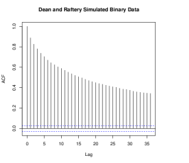
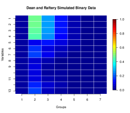
Figure 1: Diagnostic plots of the collapsed sampler applied to the simulated binary Dean and Raftery dataset, and on the right, a coincidence matrix for the sampler. The model correctly identifies 2 groups as optimal, and frequently excludes the noise variables 5 – 13.

In this section the sampler is applied to the datasets described in Section 2.2. In all cases, a pilot run was first performed, before a better individually tuned sampler was then run on each dataset, based on the sampler’s initial performance. Multiple runs of the sampler were also performed, to ensure consistency of results.

5.1 Dean and Raftery data

The algorithms described in Sections 3 and 4 were implemented in C and applied to the datasets in the R environment (R Core Team, 2013). Total run time varied depending on the size and particularly the number of variables of the dataset in question. For example, the total time taken to fit a model to the Alzheimer dataset, including post hoc parameter estimation, was about three and a half minutes. Fitting a finely tuned collapsed sampler to the larger Teaching dataset, without performing post hoc parameter estimation, took about 25 minutes, or about seven and a half times as long. Nevertheless, this should still be viewed as being reasonably efficient, as model and variable selection, as well as clustering, is simultaneously taking place.

A sampler was run on the binary simulated data for 50,000 iterations after 1,000 iterations burn-in, with 1 in 10 samples retained by subsampling. The coincidence matrix is shown on the left hand side of Figure 1. This clearly identifies a two group model with variables 1-4 as being optimal for clustering. In particular, variables 5-13 are included less than half the time, whereas variables 1-4 are included with high probability. The choice of two groups is decisively confirmed in Table LABEL:tab:DRgroup, with a posterior probability of $0.4814$. The sampler correctly classifies 381 of the 500 observations, only seven less than would be found using the true parameter values. These results are comparable to those found by Dean and Raftery (2010).

Table 4: Posterior probability for number of groups in the binary Dean and Raftery data. A two group model is correctly identified as being optimal.

$p_{1}$	$p_{2}$	$p_{3}$	$p_{4}$	$p_{5}$
0.0510	0.4814	0.2840	0.1358	0.0396

The sampler was run for 100,000 iterations after 10,000 burn-in for the non-binary data. The output was thinned and every 1 in 10 samples retained to construct the coincidence matrix shown in Figure 2. Four classes is most likely a posteriori with $p_{3}=0.2986$, $p_{4}=0.4113$ and $p_{5}=0.2146$. The four informative variables (1-4) are the only ones which the sampler indicates are worth retaining.

Table 5: Posterior probability for number of groups in the non-binary Dean and Raftery data.

$p_{2}$	$p_{3}$	$p_{4}$	$p_{5}$	$p_{6}$
0.0243	0.2986	0.4113	0.2146	0.0512

To investigate the effect of sample size on the sampler’s performance we further simulated ten datasets each with $N=1000,2500,5000,10000$ from the non-binary model. Table 6 shows the relative runtime (relative to $N=1000$), on a machine with 4 Gb RAM and 2.4GHz Intel i5 processor. The Rand index, based on how many would have been correctly predicted using the true parameter values, is also shown. It can be seen that the runtime increases roughly linearly with $N$ following the rough analysis in Section 3.4.1.

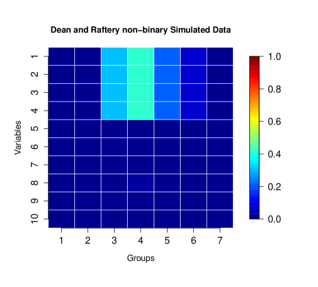
Figure 2: Summary of the spaces most commonly visited by the sampler over a run on the non-binary simulated data.

Table 6: Runtimes and Rand indices for different simulated binary Dean and Raftery datasets of size $N$.

$N$	Relative runtime	Rand index
1000	1	0.898 (0.045)
2500	2.552	0.928 (0.023)
5000	5.043	0.947 (0.032)
10000	9.767	0.960 (0.017)

5.2 Alzheimer Data

Initially, the sampler was run on the Alzheimer data for 20,000 iterations after 1,000 iterations burn-in. While a visual inspection of the log posterior suggested that good mixing was occurring, the log posterior samples were found to have high autocorrelation, and diagnostic tools suggested that a longer sampling run was required. The sampler was then run for 100,000 iterations, and thinned by subsampling every twentieth iterate. While this substantially reduced the amount of autocorrelation between samples, the results of the clustering remained relatively unaffected. Diagnostic plots of the sampling run are shown in Figure 3.

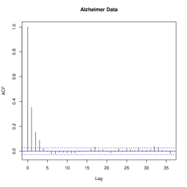
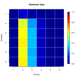
Figure 3: Diagnostic plots of the collapsed sampler applied to the Alzheimer dataset, and on the right, a coincidence matrix for the sampler. The model appears to identify 2 groups as optimal, and frequently excluded variable 1 (Hallucination) during the run.

The coincidence matrix of the sampling run is shown in the rightmost plot of Figure 3. The sampler excluded variable 1, Hallucination, a majority of the time, and identified 2 or 3 groups as optimal for the data, spending a majority of time in the 2 group space. The approximate posterior probability of a 2 group model is 0.6284, while that for a 3 group model is 0.2996 suggesting little evidence for a model with more than 2 groups. The approximate posterior of $G$ is given in Table 7.

Table 7: Posterior probability for number of groups in Alzheimer data, firstly setting $\pi=0.5$, and secondly using a Beta(1,1.5) hyperprior on $\pi$.

Setting for $\pi$	$p_{2}$	$p_{3}$	$p_{4}$	$p_{5}$	$p_{6}$
$\pi=0.5$	0.6284	0.2996	0.0622	0.0096	0.0002
$\pi{\sim}\mbox{Beta(1,1.5)}$	0.6600	0.2724	0.0584	0.0092	0

Additionally, we ran the sampler using a hyperprior on $\pi$ as outlined in Section 3.2 choosing hyperparameters $a_{0}=1$ and $b_{0}=M/4=1.5$ as outlined in Ley and Steel (2009). The posterior for the number of classes is shown in the second row of Table 7. Hallucination (variable 1) was again excluded most of the time with a 2 class model being most preferred.

We also compare parameter maximum a posteriori and posterior standard deviation estimates for the item probability parameters of a 2 group model fitted to this dataset using the collapsed sampler to those obtained using a full Gibbs sampler in the BayesLCA package. See Garrett and Zeger (2000) and Walsh (2006) for descriptions of a full model Gibbs sampler method for LCA.

Estimates from the full Gibbs sampler were obtained from 50,000 iterations after 1,000 iterations burn-in and, with every tenth sample retained. Estimates from the two methods are nearly identical. These are given in Table 8. This suggests that while the most obvious uses of the collapsed sampler are to perform model and variable selection, as well as cluster the data, it can also be used as an effective tool for parameter estimation.

Table 8: MAP item probability estimates (posterior standard deviations in parentheses) for the Alzheimer data obtained from post-hoc estimates from the collapsed Gibbs sampler and from a full model Gibbs sampler run.

Collapsed Gibbs sampler post-hoc estimates

Hallucination Activity Aggression Agitation Diurnal Affective Group 1 0.08 (0.03) 0.54 (0.06) 0.10 (0.04) 0.14 (0.06) 0.13 (0.05) 0.59 (0.08) Group 2 0.10 (0.04) 0.80 (0.06) 0.40 (0.08) 0.64 (0.12) 0.39 (0.07) 0.94 (0.04)

Full model Gibbs sampler estimates

Hallucination Activity Aggression Agitation Diurnal Affective Group 1 0.08 (0.03) 0.54 (0.06) 0.11 (0.05) 0.14 (0.06) 0.14 (0.05) 0.59 (0.08) Group 2 0.10 (0.04) 0.79 (0.07) 0.39 (0.08) 0.64 (0.12) 0.38 (0.07) 0.93 (0.07)

5.3 Teaching Styles Data

A collapsed sampler was run on the Teaching Styles data for 200,000 iterations after 5,000 iterations burn-in, with 1 in 20 samples retained by subsampling. Diagnostic tools suggest that the sampler behaves satisfactorily on the data. Diagnostic plots of the sampler are shown in Figure 4.

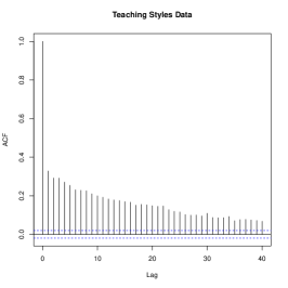
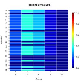
Figure 4: Diagnostic plots of the collapsed sampler applied to the Teaching Styles dataset, and on the right, a coincidence matrix for the sampler.

The coincidence matrix for the sampler is also shown as the rightmost plot in Figure 4. While several variables are decisively dropped by the sampler, a certain amount of uncertainty exists when it comes to selecting an optimal number of groups. Posterior probabilities for the number of groups are given in Table 9. These suggest most evidence for a 7 group model, with lesser (but fair) support for 6, 8 and even 9 groups. Inspection of the clusterings shows that both the 7 and 8 group models cluster some observations into quite small groups; one group in the 7 group model has only 10 observations, while the two smallest groups in the 8 group model contain only 2 and 15 observations respectively.

A cross-classification table comparison of the 6 and 7 group models is shown in Table 10. This demonstrates that the main difference between the two models from a clustering perspective is the introduction of an extra group - Group 6 in the 7 group model - which contains observations clustered to Groups 1 and 3 with high uncertainty in the 6 group model. This suggests that the additional groups in the model may improve model fit without necessarily introducing additional distinct clusters to the data.

Table 9: Posterior probability for number of groups in Teaching Styles data.

$p_{6}$	$p_{7}$	$p_{8}$	$p_{9}$	$p_{10}$	$p_{11}$
0.2071	0.3894	0.2627	0.1120	0.0257	0.0031

Table 10: Comparison of mapped clusterings for the 6 and 7 group models fitted to the Teaching Styles dataset. For convenience some rows in the table have been re-arranged to illustrate the agreement in the clusterings.

	Group 1	Group 2	Group 3	Group 4	Group 5	Group 6
Group 1	40	0	3	0	0	0
Group 2	0	59	0	0	0	0
Group 3	0	0	105	0	0	0
Group 4	1	0	6	141	0	0
Group 5	0	0	3	0	51	0
Group 6	6	0	4	0	0	0
Group 7	0	0	1	0	0	47

Figure 5 compares the dropped variables to those retained by the sampler. This shows heatmap plots of the item probability parameters for the 7 group model, firstly for the included and then the excluded variables. (Note that due to space restrictions, only every second variable index is included for the left plot.) Parameter estimates are highly similar for the excluded variables, while the behaviour of the parameters is much more varied for the included variables. While the estimates of parameters in Group 3 appear different from other groups for the excluded parameters, this is the smallest group in the clustering, and as a result standard error estimates for this group’s item probability parameters are extremely high, ranging between 35% and 43%.

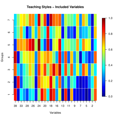
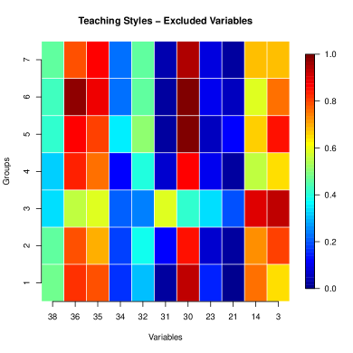
Figure 5: Heatmap plots of the item probability parameters for 7 group model fitted to the Teaching Styles data, for the included and excluded variables. Parameter estimates are highly similar for the excluded variables, while varied behaviour is apparent for included variables.

5.4 Physiotherapy Data

A collapsed sampler was run on the Physiotherapy data for 20,000 iterations after 5,000 iterations burn-in, with every second iteration retained. Auto correlation of the sampler was deemed satisfactory after these measures were taken. Diagnostic plots of the sampler are shown in Figure 6.

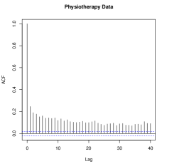
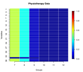
Figure 6: Diagnostic plots of the collapsed sampler applied to the Physiotherapy dataset, and on the right, a coincidence matrix for the sampler.

When applied to the full dataset, the sampler settles on 7 groups. (While a certain amount of evidence exists for an 8 group model, when compared, the two groupings have 98% agreement.) This is shown in Table 11. These 7 groups correspond well with the three pain types. A confusion matrix comparing the grouped observations with their reported pain types is shown in Table 12. Overall there is high agreement between the two sets of groupings, with a Rand index of about 92%. Note that some groups have extremely small mapped membership levels. Almost all variables proved useful in this clustering, with only one variable being dropped by the sampler. This is perhaps unsurprising, since the variables were identified for the study by expert recommendation.

Table 11: Posterior probability for number of groups in Physiotherapy data.

	$p_{7}$	$p_{8}$	$p_{9}$	$p_{10}$	$p_{11}$	$p_{12}$
	0.5577	0.3879	0.0491	0.0046	0.0006	0.0001

Table 12: Confusion matrix comparing clustered observations to reported pain types in the Physiotherapy data. (CN = Central Neuropathic, N=Nociceptive, and PN = Peripheral Neuropathic.) For convenience some rows in the table have been re-arranged to illustrate the agreement in the clusterings.

Pain Type
  CN N PN Group 1 3 0 1 Group 5 52 0 0 Group 7 30 3 0 Group 3 6 96 1 Group 6 0 120 1 Group 2 1 16 79 Group 4 3 0 13

A further study was then made to see which variables proved useful for clustering within each pain type. Samplers of length 75,000, 20,000 and 75,000 were run after 5,000 iterations of burn-in for observations reporting central neuropathic, nociceptive and peripheral neuropathic pain types respectively. For the samplers run on the central neuropathic and peripheral neuropathic datasets, the chains were thinned in a highly conservative manner, with 1 in 15 samples retained by successive subsampling. Every second iteration was retained for the nociceptive data.

In all cases, a high number of variables were decisively dropped by the samplers: 9, 15, and 18 variables were dropped for the respective datasets, with strong evidence that 21, 17 and 12 of the variables were informative to the clustering. No variables were excluded by all three models. The samplers identify 5, 4 and 3 group models as suitable for the data subsets, although again, several of the groups are quite small, particularly for the model fitted to the nociceptive data.

Comparing the clusterings of the models fitted to the data subsets to the clustering of the relevant observations from the model fitted to the full dataset, shows a high level of agreement, with Rand indices of 82%, 90% and 93% respectively. In particular, it is worth noting that when analyzing only the central neuropathic and nociceptive subsets, the number of groups chosen is the same as the number of groups used for observations on the respective pain type when analyzing the full dataset.

For the peripheral neuropathic subset, only two observations with this pain type are not placed into one of three groups, the number of groups chosen by the model fitted to the data subset.

The main difference between the clusterings is that the groups in models fitted to the data subsets are of a more equal size in comparison with the relevant subsets obtained from clustering the full dataset; this makes sense, as excluding the variables which are not meaningful for the subset in question make it easier to distinguish between different types of behaviour. A comparison of the clusterings for the nociceptive dataset is shown in Table 13.

Table 13: Confusion matrix comparing clustered observations based on the model fitted to the nociceptive subset to the clustering of the relevant observations obtained from the 7 group model applied to the full Physiotherapy dataset.

Full dataset
Nociceptive subset Group 6 Group 3 Group 2 Group 7 Group 2 107 2 0 0 Group 4 0 81 0 1 Group 1 13 4 15 0 Group 3 0 9 1 2

6 Discussion

In this paper we have introduced a model to perform LCA, including group and variable selection, in a Bayesian setting. Directly sampling the number of groups and the inclusion of variables allows for a suitable model to be chosen in a highly principled manner. While estimates of the posterior distribution of model parameters are not directly available, as they would be using a full model sampler, posterior means and standard deviations are nevertheless straightforward to calculate. Furthermore, in a Bayesian setting, the probabilistically driven search of the collapsed sampler over the discrete model space is a more computationally efficient approach than exhaustively computing information criteria.

Marginalisation of the posterior can lead to a more computationally efficient algorithm, especially when clustering and model selection are the main aims of analyst. Firstly, the fact that parameter samples are not required reduces the computational burden. Secondly, the omission of parameter sampling can lead to more efficient mixing, particularly for transdimensional moves, which in the case of variable selection, may require jumping between spaces of large dimension. We investigate this further in Appendix A.

In the latter two applications described in Section 5, some groups in the selected model contained only a small number of observations. These observations might potentially be viewed as outliers, or as being poorly described by the larger groups found by the model, rather than as distinct clusters. This is a particularly pragmatic approach to take when clustering in a model based setting, where the resultant high posterior standard deviations of model parameters for these small groups make interpretation of the group behaviour essentially meaningless.

We note that the outlined model for variable selection is somewhat limited by the conditional independence assumption of the LCA model. In other words, when a variable is proposed to be included or excluded by the sampling scheme, we are asking the question “does the proposed variable contain information about the clustering?”, rather than “does the proposed variable contain additional information about the clustering?” Thus, while non-informative variables are removed satisfactorily, for example, two informative but highly correlated variables would both be included with high probability, when perhaps the inclusion of just one would provide clustering results of similar quality. Raftery and Dean (2006) propose such a model for variable selection when clustering continuous data; the covariance parameter of a multivariate normal distribution being a natural way to model the conditional dependence between variables for this type of data.

Latent trait analysis models (see Bartholomew and Knott, 1999, for example) allow dependency between multivariate categorical data, and Gollini and Murphy (2013) have recently proposed a mixture of latent trait analyzers model which does not make the conditional independence assumption of LCA. Potentially this model could prove useful for variable selection in a clustering setting. On the other hand, implementing the model for this purpose may be more difficult than for LCA, as the likelihood is not available in closed form.

Finally, in Section 5.4 we applied the collapsed sampler to subsets of the dataset, based on additionally labelled information. In a general clustering setting, it may be of interest to determine which variables are most helpful for identifying particular groups in the data. This is a sort of unsupervised discriminant analysis which may be of future interest to further reduce the dimensionality of a dataset.

Appendix A Comparison with Reversible Jump MCMC

In this section we investigate how the performance of a collapsed Gibbs sampler compares with an RJMCMC based on using all model parameters. We divide this investigation into two tasks: selecting a) the number of classes, and b) which variables to include. We implement the approach of Pan and Huang (2013) using already available software to investigate the efficacy of RJMCMC for the former task, and outline our own approach to perform the latter for the case where the observed data is binary only. We find that the approach performs reasonably well when selecting the number of classes, although its performance is somewhat slower than that of the collapsed sampler. The implemented approach performs poorly when performing variable selection.

A.1 Number of Classes

To identify the number of groups in a dataset using RJMCMC methods, we apply software implementing the approach of Pan and Huang (2013). We applied the software to the binary and non-binary Dean and Raftery datasets described in Section 2.2, running the sampler for 100,000 iterations in both cases. All prior settings were set by default. In both cases, the non-informative variables were removed, since the sole task was to identify the correct number of classes.

As the software for this approach was implemented as a C++ programme, it can be thought of as broadly to our own collapsed sampler, which is implemented in C; for the binary and non-binary datasets, the software took roughly 25 and 90 minutes to run respectively, based on the same hardware specifications described previously. In both cases, this was markedly longer than the collapsed sampler took, despite the fact that the model was exploring the group space only, and the dimension of the data had been reduced.

The results from the samplers are shown in Table 14. In the case of the binary data, the correct number of groups is chosen as the most likely candidate, although, with a lower posterior probability in comparison to the collapsed sampler. In the case of the non-binary data, $G=2$ is incorrectly is chosen as the most likely candidate, with some level of uncertainty surrounding which model is the most suitable.

Table 14: Posterior probability for number of groups in the binary and non-binary Dean and Raftery datasets using the reversible jump approach of (Pan and Huang, 2013).

	$p_{1}$	$p_{2}$	$p_{3}$	$p_{4}$	$p_{5}$	$p_{\geq 6}$
Binary	0.12	0.39	0.27	0.22	0	0
Non-binary	0.09	0.23	0.14	0.15	0.13	0.26

A.2 Variable Selection

Recall that for the variable inclusion/exclusion step, a variable ${m^{*}}$ is selected at random from $1,\ldots,M.$ An inclusion or exclusion move is then proposed, based on the current status of the variable. In what follows, we assume that the state space has $G$ groups, and that the data is binary, so that $X_{nm}\in\{0,1\}$, for all $n=1,\ldots,N$ and $m=1,\ldots,M.$

Inclusion Step

Suppose we select a variable ${m^{*}},$ which is currently excluded from the model. For the inclusion step, dropping the variable index, we propose the following move:

1. Generate $u_{1},\dots,u_{G-1}\sim\mbox{Uniform}(-\epsilon,\epsilon),$ and set
   $u_{G}=-\sum^{G-1}_{i=1}u_{i}.$

2. Set

   $$\log\left(\frac{\theta_{1}}{1-\theta_{1}}\right)=\log\left(\frac{\beta}{1-\beta}\right)+u_{1},$$

   which is equivalent to setting

   $$\theta_{1}=\frac{\beta e^{u_{1}}}{1+\beta(e^{u_{1}}-1)}.$$

   Similarly, for $g=2,\ldots,G,$ set:

   $$\theta_{g}=\frac{\beta e^{u_{g}}}{1+\beta(e^{u_{g}}-1)}.$$

Then the proposed move is accepted with probability $\alpha$, where

$$\alpha = \min\left(1,\frac{p_{\mathrm{cl}}(\mathbf{X},\mathbf{Z}|\tilde{\mbox{\boldmath{$\theta$}}},\tilde{\mbox{\boldmath{$\nu$}}},\mbox{\boldmath{$\tau$}},G)}{p_{\mathrm{cl}}(\mathbf{X},\mathbf{Z}|\mbox{\boldmath{$\theta$}},\mbox{\boldmath{$\nu$}},\mbox{\boldmath{$\tau$}},G)}\frac{p_{\mathrm{n}}(\mathbf{X}|\tilde{\mbox{\boldmath{$\rho$}}},\tilde{\mbox{\boldmath{$\nu$}}})}{p_{\mathrm{n}}(\mathbf{X}|{\mbox{\boldmath{$\rho$}}},{\mbox{\boldmath{$\nu$}}})}\right.$$

$$\times \frac{\prod_{m\in\tilde{\mbox{\boldmath{$\nu$}}}_{\mathrm{n}}}p(\tilde{\mbox{\boldmath{$\rho$}}}_{m}|\beta)}{\prod_{m\in\mbox{\boldmath{$\nu$}}_{\mathrm{n}}}p(\mbox{\boldmath{$\rho$}}_{m}|\beta)}\frac{\prod_{g=1}^{G}\prod_{m\in\tilde{\mbox{\boldmath{$\nu$}}}_{\mathrm{cl}}}p(\tilde{\mbox{\boldmath{$\theta$}}}_{gm}|\beta)}{\prod_{g=1}^{G}\prod_{m\in\mbox{\boldmath{$\nu$}}_{\mathrm{cl}}}p(\mbox{\boldmath{$\theta$}}_{gm}|\beta)}$$

$$\times \left.\frac{\prod_{g=1}^{G}\prod_{m\in\tilde{\mbox{\boldmath{$\nu$}}}_{\mathrm{cl}}}p(\tilde{\mbox{\boldmath{$\theta$}}}_{gm}|\beta)}{\prod_{g=1}^{G}\prod_{m\in\mbox{\boldmath{$\nu$}}_{\mathrm{cl}}}p(\mbox{\boldmath{$\theta$}}_{gm}|\beta)}|{\mathcal{J}}|\times p(\xi\rightarrow\xi^{*})\right),$$

where

$$\frac{p_{\mathrm{cl}}(\mathbf{X},\mathbf{Z}|\tilde{\mbox{\boldmath{$\theta$}}},\tilde{\mbox{\boldmath{$\nu$}}},\mbox{\boldmath{$\tau$}},G)}{p_{\mathrm{cl}}(\mathbf{X},\mathbf{Z}|\mbox{\boldmath{$\theta$}},\mbox{\boldmath{$\nu$}},\mbox{\boldmath{$\tau$}},G)} = \prod^{G}_{g=1}\theta_{gm}^{S_{g{m^{*}}}}(1-\theta_{g{m^{*}}})^{S^{C}_{g{m^{*}}}},$$

$$\frac{p_{\mathrm{n}}(\mathbf{X}|\tilde{\mbox{\boldmath{$\rho$}}},\tilde{\mbox{\boldmath{$\nu$}}})}{p_{\mathrm{n}}(\mathbf{X}|{\mbox{\boldmath{$\rho$}}},{\mbox{\boldmath{$\nu$}}})} = \frac{1}{\rho_{m^{*}}^{N_{m^{*}}}(1-\rho_{m^{*}})^{N-N_{m^{*}}}},$$

$$\frac{\prod_{m\in\tilde{\mbox{\boldmath{$\nu$}}}_{\mathrm{n}}}p(\tilde{\mbox{\boldmath{$\rho$}}}_{m}|\beta)}{\prod_{m\in\mbox{\boldmath{$\nu$}}_{\mathrm{n}}}p(\mbox{\boldmath{$\rho$}}_{m}|\beta)} = \frac{\Gamma(\beta)^{2}}{\Gamma({2\beta})}\times\frac{1}{\rho_{m^{*}}^{\beta-1}(1-\rho_{m^{*}}^{\beta-1})},$$

$$\frac{\prod_{g=1}^{G}\prod_{m\in\tilde{\mbox{\boldmath{$\nu$}}}_{\mathrm{cl}}}p(\tilde{\mbox{\boldmath{$\theta$}}}_{gm}|\beta)}{\prod_{g=1}^{G}\prod_{m\in\mbox{\boldmath{$\nu$}}_{\mathrm{cl}}}p(\mbox{\boldmath{$\theta$}}_{gm}|\beta)} = G\frac{\Gamma(2\beta)}{\Gamma(\beta)^{2}}\prod^{G}_{g=1}\theta_{gm^{*}}^{\beta-1}(1-\theta_{gm^{*}})^{\beta-1},$$

and we define $S_{g{m^{*}}}=\sum^{N}_{n=1}X_{nm^{*}}Z_{ng},$ $S^{C}_{g{m^{*}}}=\sum^{N}_{n=1}(1-X_{nm^{*}})Z_{ng},$ and $N_{m^{*}}=\sum^{N}_{n=1}X_{nm^{*}}.$ Here we use $p(\xi\rightarrow\xi^{*})=1/M$ to denote the probability of the proposed move. Finally, the Jacobian ${\mathcal{J}}$ is defined as ${\mathcal{J}}_{1g}=\frac{\partial\theta_{gm^{*}}}{\partial\rho_{m^{*}}},$ and ${\mathcal{J}}_{kg}=\frac{\partial\theta_{gm^{*}}}{\partial u_{k-1}},$ for $g=1,\dots,G\mbox{ and }k=2,\dots,G.$

Exclusion Step

If the variable ${m^{*}},$ is currently included in the model, we propose the exclusion step,

$$\rho=\frac{\left(\prod^{G}_{g=1}\theta_{g}\right)^{1/G}}{\left(\prod^{G}_{g=1}\theta_{g}\right)^{1/G}+\left(\prod^{G}_{g=1}(1-\theta_{g})\right)^{1/G}},$$

where again we have dropped the variable index. Using this expression, we then obtain

$$u_{g}=\left(1-\frac{1}{G}\right)\log\left(\frac{\theta_{g}}{1-\theta_{g}}\right)-\frac{1}{G}\sum_{j\neq g}\log\left(\frac{\theta_{j}}{1-\theta_{j}}\right),$$

for $g=1,\ldots,G-1$, demonstrating the required bijection between $\mbox{\boldmath{$\theta$}}_{m^{*}}$ and $(\rho_{m^{*}},\mathbf{u})$. The proposed move is again accepted with probability $\alpha$, where

$$\alpha = \min\left(1,\frac{p_{\mathrm{cl}}(\mathbf{X},\mathbf{Z}|\tilde{\mbox{\boldmath{$\theta$}}},\tilde{\mbox{\boldmath{$\nu$}}},\mbox{\boldmath{$\tau$}},G)}{p_{\mathrm{cl}}(\mathbf{X},\mathbf{Z}|\mbox{\boldmath{$\theta$}},\mbox{\boldmath{$\nu$}},\mbox{\boldmath{$\tau$}},G)}\frac{p_{\mathrm{n}}(\mathbf{X}|\tilde{\mbox{\boldmath{$\rho$}}},\tilde{\mbox{\boldmath{$\nu$}}})}{p_{\mathrm{n}}(\mathbf{X}|{\mbox{\boldmath{$\rho$}}},{\mbox{\boldmath{$\nu$}}})}\right.$$

$$\times \frac{\prod_{m\in\tilde{\mbox{\boldmath{$\nu$}}}_{\mathrm{n}}}p(\tilde{\mbox{\boldmath{$\rho$}}}_{m}|\beta)}{\prod_{m\in\mbox{\boldmath{$\nu$}}_{\mathrm{n}}}p(\mbox{\boldmath{$\rho$}}_{m}|\beta)}\frac{\prod_{g=1}^{G}\prod_{m\in\tilde{\mbox{\boldmath{$\nu$}}}_{\mathrm{cl}}}p(\tilde{\mbox{\boldmath{$\theta$}}}_{gm}|\beta)}{\prod_{g=1}^{G}\prod_{m\in\mbox{\boldmath{$\nu$}}_{\mathrm{cl}}}p(\mbox{\boldmath{$\theta$}}_{gm}|\beta)}$$

$$\times \left.\frac{\Gamma(\beta)^{2}}{G\Gamma(2\beta)}\times\frac{1}{\prod^{G}_{g=1}\theta_{gm^{*}}^{\beta-1}(1-\theta_{gm^{*}})^{\beta-1}}|{\mathcal{J}}|\times p(\xi\rightarrow\xi^{*})\right)$$

where the calculations are inverted, so that

$$\frac{p_{\mathrm{cl}}(\mathbf{X},\mathbf{Z}|\tilde{\mbox{\boldmath{$\theta$}}},\tilde{\mbox{\boldmath{$\nu$}}},\mbox{\boldmath{$\tau$}},G)}{p_{\mathrm{cl}}(\mathbf{X},\mathbf{Z}|\mbox{\boldmath{$\theta$}},\mbox{\boldmath{$\nu$}},\mbox{\boldmath{$\tau$}},G)} = \frac{1}{\prod^{G}_{g=1}\theta_{gm}^{S_{g{m^{*}}}}(1-\theta_{g{m^{*}}})^{S^{C}_{g{m^{*}}}}},$$

$$\frac{p_{\mathrm{n}}(\mathbf{X}|\tilde{\mbox{\boldmath{$\rho$}}},\tilde{\mbox{\boldmath{$\nu$}}})}{p_{\mathrm{n}}(\mathbf{X}|{\mbox{\boldmath{$\rho$}}},{\mbox{\boldmath{$\nu$}}})} = \rho_{m^{*}}^{N_{m^{*}}}(1-\rho_{m^{*}})^{N-N_{m^{*}}},$$

$$\frac{\prod_{m\in\tilde{\mbox{\boldmath{$\nu$}}}_{\mathrm{n}}}p(\tilde{\mbox{\boldmath{$\rho$}}}_{m}|\beta)}{\prod_{m\in\mbox{\boldmath{$\nu$}}_{\mathrm{n}}}p(\mbox{\boldmath{$\rho$}}_{m}|\beta)} = \frac{\Gamma({2\beta})}{\Gamma(\beta)^{2}}{\rho_{m^{*}}^{\beta-1}(1-\rho_{m^{*}}^{\beta-1})},$$

$$\frac{\prod_{g=1}^{G}\prod_{m\in\tilde{\mbox{\boldmath{$\nu$}}}_{\mathrm{cl}}}p(\tilde{\mbox{\boldmath{$\theta$}}}_{gm}|\beta)}{\prod_{g=1}^{G}\prod_{m\in\mbox{\boldmath{$\nu$}}_{\mathrm{cl}}}p(\mbox{\boldmath{$\theta$}}_{gm}|\beta)} = \frac{\Gamma(\beta)^{2}}{G\Gamma(2\beta)}\times\frac{1}{\prod^{G}_{g=1}\theta_{gm^{*}}^{\beta-1}(1-\theta_{gm^{*}})^{\beta-1}}.$$

The probability of the proposed move remains, $p(\xi\rightarrow\xi^{*})=1/M$.

Dean and Raftery Data Application

We apply this approach to the binary Dean and Raftery dataset described previously in Section 2.2. Here, we fix the number of groups to the true value $G=2$, so that the model search is based on variable selection only. The sampler was run for 50,000 iterations, with $\epsilon=1$, which resulted in an acceptance probability for the inclusion/exclusion move of $\alpha\approx 0.12.$

The posterior probability for variable inclusion from the sampler are shown in Table 15. None of the informative variables are selected as frequently as for the collapsed sampler, with the model only finding weak evidence for variable 1, and failing to distinguish between the other variables.

Table 15: Posterior probability for variable inclusion in the binary Dean and Raftery data using RJMCMC.

	$\mathbb{P}(\mbox{Inclusion})$
Variable 1	0.62
Variable 2	0.51
Variable 3	0.53
Variable 4	0.55
Variable 5	0.48
Variable 6	0.53
Variable 7	0.51
Variable 8	0.46
Variable 9	0.48
Variable 10	0.52
Variable 11	0.52
Variable 12	0.50
Variable 13	0.49

References

- Aitkin et al (1981) Aitkin M, Anderson D, Hinde J (1981) Statistical modelling of data on teaching styles. Journal of the Royal Statistical Society, Series A 144:419–461
- Akaike (1973) Akaike H (1973) Information theory and an extension of the maximum likelihood principle. In: Second International Symposium on Information Theory, Akadémiai Kiadó, pp 267–281
- Bartholomew and Knott (1999) Bartholomew DJ, Knott M (1999) Latent Variable Models and Factor Analysis, 2nd edn. Kendall’s Library of Statistics, Hodder Arnold
- Bennet (1976) Bennet N (1976) Teaching Styles and Pupil Progress. Open Books, London
- Bensmail et al (1997) Bensmail H, Celeux G, Raftery A, Robert C (1997) Inference in model-based cluster analysis. Statistics and Computing 7:1–10
- Cappé et al (2003) Cappé O, Robert CP, Rydén T (2003) Reversible jump, birth-and-death and more general continuous time Markov chain Monte Carlo samplers. Journal of the Royal Statistical Society: Series B (Statistical Methodology) 65(3):679–700
- Carpaneto and Toth (1980) Carpaneto G, Toth P (1980) Algorithm 548: Solution of the Assignment Problem [H]. ACM Transactions on Mathematical Software 6:104–111
- Celeux et al (2000) Celeux G, Hurn M, Robert CP (2000) Computational and inferential difficulties with mixture posterior distributions. Journal of the American Statistical Association 95:957–970
- Celeux et al (2006) Celeux G, Forbes F, Robert CP, Titterington D (2006) Deviance information criteria for missing data models. Bayesian Analysis 1:651–673
- Chopin and Robert (2010) Chopin N, Robert CP (2010) Properties of nested sampling. Biometrika 97(3):741–755
- Dean and Raftery (2010) Dean N, Raftery AE (2010) Latent Class Analysis Variable Selection. The Annals of the Institute of Statistical Mathematics 62:11–35
- Dellaportas and Papageorgiou (2006) Dellaportas P, Papageorgiou I (2006) Multivariate mixtures of normals with unknown number of components. Statistics and Computing 16:57–68
- Dempster et al (1977) Dempster AP, Laird NM, Rubin DB (1977) Maximum Likelihood from Incomplete Data via the EM Algorithm. Journal of the Royal Statistical Society B 39:1–38
- Fraley and Raftery (2007) Fraley C, Raftery A (2007) Model-Based Methods of Classification: Using the Software in Chemometrics. Journal of Statistical Software 18:1–13
- Frühwirth-Schnatter (2004) Frühwirth-Schnatter S (2004) Estimating marginal likelihoods for mixture and Markov switching models using bridge sampling techniques. Econometrics Journal 7(1):143–167
- Frühwirth-Schnatter (2006) Frühwirth-Schnatter S (2006) Finite Mixture and Markov Switching Models: Modeling and Applications to Random Processes. Springer
- Garrett and Zeger (2000) Garrett ES, Zeger SL (2000) Latent Class Model Diagnosis. Biometrics 56:pp. 1055–1067
- Geman and Geman (1984) Geman S, Geman D (1984) Stochastic Relaxation, Gibbs Distributions and the Bayesian Restoration of Images. IEEE Transactions on Pattern Analysis and Machine Intelligence 6:721–741
- Geweke (1989) Geweke J (1989) Bayesian inference in econometric models using Monte Carlo integration. Econometrica 57(6):pp. 1317–1339
- Gollini and Murphy (2013) Gollini I, Murphy T (2013) Mixture of latent trait analyzers for model-based clustering of categorical data. Statistics and Computing (to appear)
- Goodman (1974) Goodman LA (1974) Exploratory latent structure analysis using both identifiable and unidentifiable models. Biometrika 61:215–231
- Green (1995) Green P (1995) Reversible jump Markov chain Monte Carlo computation and Bayesian model determination. Biometrika 82:711–732
- Kass and Raftery (1995) Kass RE, Raftery AE (1995) Bayes Factors. Journal of the American Statistical Association 90:773–795
- Ley and Steel (2009) Ley E, Steel MFJ (2009) On the effect of prior assumptions in Bayesian model averaging with applications to growth regression. Journal of Applied Econometrics 24:651–674
- Marin et al (2005) Marin JM, Mengersen K, Robert CP (2005) Bayesian modelling and inference on mixtures of distributions. In: Dey D, Rao C (eds) Bayesian Thinking: Modeling and Computation, Handbook of Statistics, vol 25, 1st edn, North Holland, Amsterdam, chap 16, pp 459–507
- McDaid et al (2013) McDaid AF, Murphy TB, Friel N, Hurley N (2013) Improved Bayesian inference for the stochastic block model with application to large networks. Computational Statistics & Data Analysis 60:12 – 31
- McLachlan and Peel (2002) McLachlan G, Peel D (2002) Finite Mixture Models. John Wiley & Sons
- Meng and Wong (1996) Meng XL, Wong WH (1996) Simulating ratios of normalizing constants via a simple identity: A theoretical exploration. Statistica Sinica 6:831 – 860
- Moran et al (2004) Moran M, Walsh C, Lynch A, Coen RF, Coakley D, Lawlor BA (2004) Syndromes of Behavioural and Psychological Symptoms in Mild Alzheimer’s Disease. International Journal of Geriatric Psychiatry 19:359–364
- Newton and Raftery (1994) Newton MA, Raftery AE (1994) Approximate bayesian inference with the weighted likelihood bootstrap. Journal of the Royal Statistical Society Series B (Methodological) 56(1):pp. 3–48
- Nobile (2005) Nobile A (2005) Bayesian finite mixtures: a note on prior specification and posterior computation. Tech. Rep. 05-3, University of Glasgow, Glasgow, UK
- Nobile and Fearnside (2007) Nobile A, Fearnside A (2007) Bayesian Finite Mixtures with an Unknown Number of Components: The Allocation Sampler. Statistics and Computing 17:147–162
- Pan and Huang (2013) Pan JC, Huang GH (2013) Bayesian inferences of latent class models with an unknown number of classes. Psychometrika pp 1–26
- Pandolfi et al (2014) Pandolfi S, Bartolucci F, Friel N (2014) A generalized multiple-try version of the reversible jump algorithm. Computational Statistics & Data Analysis 72(0):298 – 314
- Plummer et al (2006) Plummer M, Best N, Cowles K, Vines K (2006) CODA: Convergence diagnosis and output analysis for MCMC. R News 6:7–11
- R Core Team (2013) R Core Team (2013) R: A Language and Environment for Statistical Computing. R Foundation for Statistical Computing, Vienna, Austria, URL http://www.R-project.org/
- Raftery and Dean (2006) Raftery AE, Dean N (2006) Variable selection for model-based clustering. Journal of the American Statistical Association 101:168–178
- Raftery et al (2007) Raftery AE, Newton MA, Satagopan JM, Krivitsky PN (2007) Estimating the integrated likelihood via posterior simulation using the harmonic mean identity (with discussion). In: Bernardo J, Bayarri M, Berger J, Dawid A, Heckerman D, Smith A, West M (eds) Bayesian Statistics 8, Oxford University Press, Oxford, pp 1–45
- Richardson and Green (1997) Richardson S, Green PJ (1997) On Bayesian Analysis of Mixtures with an Unknown Number of Components (with discussion). Journal of the Royal Statistical Society, Series B (Statistical Methodology) 59:731–792
- Rousseau and Mengersen (2011) Rousseau J, Mengersen K (2011) Asymptotic behaviour of the posterior distribution in overfitted mixture models. Journal of the Royal Statistical Society, Series B (Statistical Methodology) 73:689–710
- Schwarz (1978) Schwarz G (1978) Estimating the Dimension of a Model. The Annals of Statistics 6:461–464
- Smart et al (2011) Smart KM, Blake C, Staines A, Doody C (2011) The Discriminative Validity of “Nociceptive”, “Peripheral Neuropathic”, and “Central Sensitization” as Mechanisms-based Classifications of Musculoskeletal Pain. Clinical Journal of Pain 27:655 – 663
- Spiegelhalter et al (2002) Spiegelhalter DJ, Best NG, Carlin BP, van der Linde A (2002) Bayesian Measures of Model Complexity and Fit. Journal of the Royal Statistical Society, Series B 64:583–639
- Stephens (2000a) Stephens M (2000a) Bayesian analysis of mixture models with an unknown number of components an alternative to reversible jump methods. The Annals of Statistics 28(1):40–74
- Stephens (2000b) Stephens M (2000b) Dealing with Label Switching in Mixture Models. Journal of the Royal Statistical Society, Series B 62:795–809
- Tadesse et al (2005) Tadesse MG, Sha N, Vannucci M (2005) Bayesian Variable Selection in Clustering High-Dimensional Data. Journal of American Statistical Association 100:602–617
- Walsh (2006) Walsh C (2006) Latent Class Analysis Identification of Syndromes in Alzheimer’s Disease: A Bayesian Approach. Metodološki Zvezki - Advances in Methodology and Statistics 3:147 – 162
- White and Murphy (2013) White A, Murphy B (2013) BayesLCA: Bayesian Latent Class Analysis. URL http://CRAN.R-project.org/package=BayesLCA, R package version 1.3
- Wyse and Friel (2012) Wyse J, Friel N (2012) Block Clustering with Collapsed Latent Block Models. Statistics and Computing 22:415–428