A continuous model for bosonic hard spheres in quasi one-dimensional optical lattices

Abstract

By means of diffusion Monte Carlo calculations, we investigated the quantum phase transition between a superfluid and a Mott insulator for a system of hard-sphere bosons in a quasi one-dimensional optical lattice. For this continuous hamiltonian, we studied how the stability limits of the Mott phase changed with the optical lattice depth and the transverse confinement width. A comparison of these results to those of a one-dimensional homogeneous Bose-Hubbard model indicates that this last model describes accurately the phase diagram only in the limit of deep lattices. For shallow ones, our results are comparable to those of the sine-Gordon model in its limit of application. We provide an estimate of the critical parameters when none of those models are realistic descriptions of a quasi one-dimensional optical lattice.

I INTRODUCTION

When a pair of laser beams interfere to produce a standing wave, the net effect is the generation of a periodic potential in whose minima alkali metal atoms can be trapped bloch1 ; bloch2 ; greiner . If we use more than a single pair of laser beams, those potential minima can be regularly located to form a three dimensional pattern called “optical lattice”. The defining parameters of these structures are the potential depth, $V_{0}$, the distance between potential minima, $\lambda/2$, and their distribution in space. Here, $\lambda$ is the wavelength of the laser and determines another relevant quantity, the recoil energy, $E_{R}=h^{2}/2m\lambda^{2}$ ($h$, Planck constant; $m$, mass of the atom). Optical lattices of almost any geometry can be built bloch3 , but quasi one-dimensional (quasi 1D) ones have been experimentally favored paredes ; haller ; stoferle ; clement ; kruger ; fabri in the hopes of obtaining a Tonks-Girardeau (TG) gas paredes ; kinoshita ; cazalilla .

Almost all the theoretical treatment of optical lattices has been made using as a reference the Bose-Hubbard model (BH) bloch2 ; cazalilla . This is a discrete model whose defining parameters, $J$ and $U$, can be deduced from a more general continuous hamiltonian through a series of approximations jaksch . However, in this work, instead of that model, we have used continuous hamiltonians as the ones already employed to describe neutral atoms loaded in harmonic traps cazalilla ; dun ; gir ; gregori ; blume ; gregori2 ; pollet or homogeneous systems gregori3 ; boro , to represent the quasi one-dimensional optical lattices we are interested in. To our knowledge, a similar approach has only been used for full three dimensional (3D) arrangements pilati , and for strictly one-dimensional ones feli1 ; feli2 .

It can be shown bloch2 that the optical lattice potential has the form:

$$V_{ext}(x,y,z)=V_{x}\sin^{2}(k_{x}x)+V_{y}\sin^{2}(k_{y}y)+V_{z}\sin^{2}(k_{z}z)$$ (1)

in which the parameters $V_{x},V_{y}$ and $V_{z}$, could be different in the three spatial directions. To generate a quasi one-dimensional system, the standard practice paredes ; haller ; stoferle ; clement ; kruger ; fabri is to start with a very high and common value ($V_{x}=V_{y}=V_{z}$ = 20-40$E_{R}$), and relax one of them afterwards. The chosen one defines the longitudinal axis of the optical lattice. This means that, for instance, we can express the external potential as:

$$V_{ext}(x,y,z)=V_{0}\sin^{2}(kz)+\frac{1}{2}m\omega_{\perp}^{2}(x^{2}+y^{2})\ ,$$ (2)

where $\omega_{\perp}$ is the transversal frequency of the confining harmonic potential (we have made $V_{z}=V_{0}$), and $k=2\pi/\lambda$. The full 3D hamiltonian is then:

$$H=\sum_{i=1}^{N}\left[-\frac{\hbar^{2}}{2m}\nabla^{2}+V_{ext}(x_{i},y_{i},z_{i})\right]+\sum_{i<j}V(r_{ij})\,$$ (3)

where $N$ is the number of particles of mass $m$ loaded in the quasi 1D optical lattice, and $r_{ij}$ stands for the distance between each pair. $V(r_{ij})$ is the interparticle potential, for which we used a hard spheres (HS) interaction (a common approach). This implies $V_{int}(r_{ij})=+\infty$ if $r_{ij}<a$ and 0 otherwise. $a$ is here the diameter of the hard sphere. This parameter is sometimes named $a_{3D}$ in the literature gregori2 ; gregori3 and models the scattering length of the alkali bosons loaded in the optical lattice. In this work, we solved this full hamiltonian, not a strictly one-dimensional one.

Our goal will be to compare the onset of the superfluid-Mott insulator transition (see below) in a pure 1D Bose-Hubbard model and in the more realistic hamiltonian given by Eq. (3). Since a pure 1D BH model is itself an approximation jaksch , it is useful to establish numerically the $V_{0}$ range in which it could be used as a substitute for a continuous hamiltonian. We will also solve the Schrödinger equation for the hamiltonian in Eq. (3) for ”shallow” (small $V_{0}$’s) lattices, a situation in which the BH model is not longer valid, but where the sine-Gordon model sine is a good representation for the optical lattice in strictly 1D environments. We found that our results were similar to those of the Bose-Hubbard and sine-Gordon models in their respective limits of high and low $V_{0}$’s, and can be used to describe the no-man’s land in between.

The method to solve the hamiltonian in Eq. (3) will be described in the following section. Next, and for the sake of comparison, we will display some results for quasi one dimensional systems with $V_{0}$=0. The stability limits of the Mott insulator phase for different optical lattices will be displayed next, together with a numerical comparison with those derived from the Bose-Hubbard and sine-Gordon models. We will end with some conclusions.

II METHOD

To solve the Schrödinger equation for the hamiltonian given in Eq. (3), we used a Diffusion Monte Carlo (DMC) algorithm. This technique allowed us to obtain numerically the ground state of all the boson arrangements we were interested in. Those ground states are expected to be reasonable approximations to the experimental systems, due to the extremely low temperatures typical of optical lattice studies. The numerical solution derived from DMC is exact within the statistical uncertainties derived from the use of the so called trial function boro94 . This is an initial approximation to the ground state wave function that guides the sampling of the phase space. In our case,

$$\Phi({\bf r_{1}},\cdots,{\bf r_{N}})=\prod_{i=1}^{N}\psi(x_{i},y_{i})\prod_{j=1}^{N}\phi(z_{i})\prod_{l<m=1}^{N}\Psi(r_{lm})$$ (4)

where r_i$(x_{i},y_{i},z_{i})$ are the positions of each of the $i$ neutral atoms in the optical lattice. $\psi(x_{i},y_{i})$ is the exact solution of the transversal potential. i.e., a Gaussian whose variance is related to the harmonic confining frequency $\omega_{\perp}$ by $\sigma^{2}=\frac{\hbar}{m\omega_{\perp}}$. $\sigma$ is commonly used as a measure of the width of the quasi one-dimensional confining “tube” ols ; gregori ; blume ; gregori2 ; gregori3 . Following Ref. feli1, , $\phi(z_{i})$ is the ground state wave function of a single particle under a external potential given by $V_{ext}(z)=V_{0}\sin^{2}(kz)$, while for the remaining part of the trial function we used

$$\Psi(r_{ij})=\left\{\begin{array}[]{lr}0&r_{ij}<a\\ 1-\exp(-\beta(r_{ij}-a))&r_{ij}\geq a.\end{array}\right.$$ (5)

Here, $\beta$ is a variational constant that minimizes the energy per particle at each density and $\sigma$.

In our calculations, we considered $\sigma$’s in the range $a$ - 30$a$, $a$ being the diameter of the hard sphere. Three wavelengths, $\lambda/a=50,100,200$ (given in reduced units) were used. Those values of $\lambda/a$ are in the range of the experimental ones for both ⁸⁷Rb and ¹³³Cs paredes ; haller ; fol ; gem ; bakr . To produce the densities displayed in the figures below, we used simulation cells of length 20$\lambda/a$ and a variable number of particles, ranging from zero to twice the number of the potential minima (a maximum of 80 particles in 40 wells). All the energies will be given in units of $E_{R}$, the recoil energy defined above.

III RESULTS

III.1 $V_{0}$ = 0

In Fig. (1), we considered several hard spheres arrangements with quasi one-dimensional confinement but no optical lattice in the longitudinal direction ($V_{0}$ = 0 in Eq. (2)). This is a full 3D system, whose energies per particle are displayed after the subtraction of the corresponding to the harmonic trap ($E_{HO}=\hbar\omega_{\perp}$). If we go from top to bottom in Fig. (1) the confinement becomes looser, from $\sigma/a$ = 1 for the upper curve, to $\sigma/a$ =17.78 for the lowest one. Those results are not strictly comparable to those of Refs. gregori, ; blume, ; gregori2, , since in those works the 3D hamiltonian includes an additional harmonic confinement in the longitudinal direction (of frequency $\omega_{z}$), which is absent here. However, Ref. gregori2, gives us a result qualitatively similar to the one displayed in Fig. (1): when $\sigma\sim a$, for a HS interaction and $\omega_{z}/\omega_{\perp}=$ 0.01, the longitudinal energy per particle is larger than the corresponding to a TG gas ($E=\pi^{2}\hbar^{2}n^{2}/6m$; $n=N/L$, $L$ length of the simulation cell containing the $N$ particles). On the other hand, when $\sigma/a>1$, the energy per particle is lower than the one for that pure 1D limit. This is exactly what is displayed in Fig. (1). In addition, we can see that for all confinements the energies per particle increase smoothly with $n$, in stark contradiction to what will happen when $V_{0}/E_{R}\neq 0$. This monotonous increase of the energy with the density is characteristic of a fluid. In any case, we have to bear in mind that our results are not strictly comparable to those of a TG gas, since this is a purely 1D model. In addition, the size of the particles in a TG model is supposed to be zero, i.e., a TG gas is made of “hard points” instead of hard spheres.

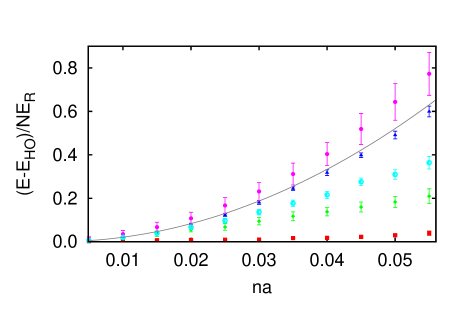
Figure 1: (Color online) Energy per particle (in units of $E_{R}$ and after subtracting the corresponding harmonic oscillator one) for $V_{0}/E_{R}=0$ versus the longitudinal density, $na$, for different transversal confinements. Full squares, $\sigma/a=17.78$; diamonds, $\sigma/a=5.62$; lower circles, $\sigma/a=3.16$; triangles, $\sigma/a=1.78$; upper circles, $\sigma/a=1$. We show also the result for a 1D TG gas as a full line.

III.2 Superfluid to Mott Insulator phase transition

As an example of the behavior of the energy as a function of the transverse confinement in an optical lattice, we display in Fig. (2) the case for $V_{0}/E_{R}=6.3$ for several values of $\sigma/a$. The density is shown as filling fraction ($n\lambda/2$), the average number of atoms per potential well. In this figure, $\lambda/a$ = 50, but the trend is common to many other values of $V_{0}/E_{R}$ and $\sigma/a$. In this particular case, we observe that the slope of the energy per particle, when it is represented as a function of the density, can change around $n\lambda/2$ = 1. This is due to the interaction between atoms inside the same potential well. From the energy slope and the energy per particle at density $n$, we can obtain the chemical potential, $\mu$, through,

$$\frac{\mu}{E_{R}}=\frac{\partial\frac{E}{E_{R}}}{\partial N}=n\frac{\partial\frac{E}{NE_{R}}}{\partial n}+\frac{E}{NE_{R}}.$$ (6)

Eq.  (6) implies that when the energy slope changes at a particular density, a discontinuity in the chemical potential is produced. Following Refs. bloch2, ; feli1, ; batrou1, ; batrou2, ; laz, , we used the appearance of that discontinuity as a signature for the existence of an incompressible ($\Delta n/\Delta\mu$ = 0) Mott insulator phase at $n\lambda/2$ = 1 bloch2 . Not all systems exhibit such discontinuity in $\mu$; $V_{0}/E_{R}$ has to reach a particular limit before we can see that change. To obtain that critical value, we considered arrangements with different $V_{0}/E_{R}$, $\sigma/a$, and $\lambda/a$’s, and calculated their chemical potentials just below and above $n\lambda/2$ = 1. We did that by performing third order polynomial fits to the energy per particle vs. density for filling fractions in the ranges [0.9:1] and [1:1.1] and applying Eq. (6) at a filling fraction of one. We considered both values of $\mu/E_{R}$ to be identical if their differences were lower than their respective error bars, obtained from the least squares fits. The critical value for the appearance of a Mott insulator phase, ($V_{0}/E_{R}$)_C, was calculated as the average between the last $V_{0}/E_{R}$ at which the $\mu$’s are identical, and the first one at which they are not. An example of this entire procedure is given in Fig. (3). The existence of size effects was checked by performing calculations with bigger simulation cells (80 potential wells and $\sim$ 80 atoms), and found negligible.

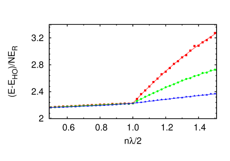
Figure 2: (Color online) Same as in previous figure, but for arrangements with $V_{0}/E_{R}=6.3$. The density is displayed as the filling fraction for different $\left(\sigma/a\right)$ values. Squares, $\sigma/a=1.78$; circles, $\sigma/a=3.16$; triangles, $\sigma/a=5.62$. Lines are third order polynomial fits and are intended as guides-to-the eye. Error bars are of the same size as the symbols and were not displayed for simplicity.

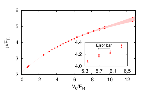
Figure 3: (Color online). Values of $\mu/E_{R}$ calculated using Eq. (6) for densities above (upper symbols) and below (lower symbols) at $n\lambda/2=1$. In this example, $\lambda/a$ = 50 and $\sigma/a\sim 8$. From this set of results, $(V_{0}/E_{R})_{C}=5.8\pm 0.2$.

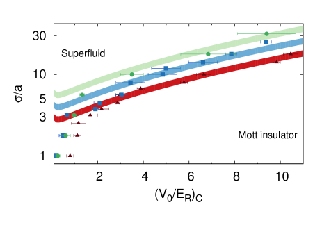
Figure 4: (Color online). Critical values of $\left(V_{0}/E_{R}\right)_{C}$ for different $\left(\sigma/a\right)$’s. Triangles, squares and circles show the simulation results for $\lambda/a=50$, $\lambda/a=100$ and $\lambda/a=200$, respectively. The three stripes correspond to the $\left(V_{0}/E_{R}\right)_{C}$’s values predicted for the 1D BH model for each $\lambda/a$ considered. From top to bottom, $\lambda/a=200$, $\lambda/a=100$ and $\lambda/a=50$.

Fig. (4) gives the critical values of $V_{0}/E_{R}$ obtained from the above procedure for three different $\lambda/a$’s (50,100 and 200), and a number of $\sigma/a$’s. What we see is that for similar $\omega_{\perp}$’s, an increase in $\lambda$ (and obviously in the distance between potential wells) reduces the value of $\left(V_{0}/E_{R}\right)_{C}$ necessary to produce a Mott insulator phase. This is exactly the opposite to what happens in a 3D arrangement, where an increase in $\lambda$ stabilizes the fluid phase of the atoms loaded in the optical lattice pilati . In Fig. (4) we can observe also another trend: when $\sigma/a$ decreases, i.e. when the confinement “tube” is thinner, $\left(V_{0}/E_{R}\right)_{C}$ decreases, becoming approximately zero for $\sigma/a$ = 1. This is in agreement with the results for the strictly 1D system of Ref. feli2, . There, one can see that $\left(V_{0}/E_{R}\right)_{C}$ is exactly zero, i.e., even an infinitesimally small value of $V_{0}$ is enough to pin the atoms to their respective potential wells and create a Mott insulator at $n\lambda/2$ = 1. The same conclusion is reached when these systems are modeled by a sine-Gordon model sine .

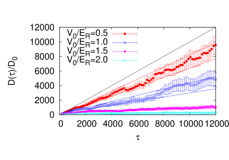
Figure 5: (Color online). Diffusion of the center of mass for $\sigma/a\ =1.78$ and $\lambda/a=50$ for several $V_{0}/E_{R}$ values (in the legend). The data have been normalized so that the slope of the curve is the superfluid fraction. The black line corresponding to a 100% superfluid fraction has been included for reference. The different bands displayed are the results of performing least squares linear fits to the respective sets of points defined by the upper and lower limits of the error bars.

The simulation results displayed in Fig. (4) define two regions for $n\lambda/2$ = 1. In the lower region we have the incompressible Mott insulator phase defined above, while the upper part of the figure is labeled “superfluid”. The superfluid fraction of a bosonic system can be extracted from DMC simulations by an extension of the winding number technique PhysRevLett.74.1500 ; PhysRevB.73.224515 as,

$$\frac{\rho_{s}}{\rho}=\lim_{\tau\to\infty}\frac{D(\tau)}{\tau D_{0}}$$ (7)

with $D_{0}=\hbar^{2}/2m$, and

$$D(\tau)=\frac{1}{2dN}\langle\left(\vec{r}_{CM}(\tau)-\vec{r}_{CM}(0)\right)^{2}\rangle\ .$$ (8)

where $N$ is the number of particles and $d$ the dimension of the system. $\vec{r}_{CM}(\tau)$ is the position of the center of mass of all the particles. A correct application of Eq. (8) requires that when an atom goes out of the simulation cell, one has to keep track of the evolution of the center of mass beyond the simulation cell limits. $\tau$ is a measure of the number of simulation steps from the point in which we start to collect statistics ($\tau=0$). When each atom is located in a particular potential well, the superfluid fraction is zero for infinitely large simulation times. In Fig. (5) we display the results for this estimator in the case $\sigma/a$ = 1.78 and $\lambda/a=50$ for different values of $V_{0}/E_{R}$. The slopes in Fig. (5) allow us to obtain superfluid fractions of $0.67\pm 0.05$ for $V_{0}/E_{R}=0.5$, $0.32\pm 0.07$ for $V_{0}/E_{R}=1$, $0.06\pm 0.01$ for $V_{0}/E_{R}=1.5$ and $0.02\pm 0.01$ for $V_{0}/E_{R}=2$. Since the $(V_{0}/E_{R})_{C}$ value for the same conditions in Fig. (4) is 1.1 $\pm$ 0.2, this means that at $n\lambda/2=1$ the onset of the appearance of the Mott insulator is correlated with a virtual disappearance of the superfluid fraction. The quantum phase transition is then a superfluid-Mott insulator one. For densities other than $n\lambda/2=1$ the system behaves always as a superfluid.

III.3 Comparison with a Bose-Hubbard model

The Bose-Hubbard model is a de facto standard to study the physics of atoms in optical lattices, to the extent that many experimental data are given in terms of $J$ and $U$, its defining parameters, instead of using the real experimental value, $V_{0}$. The hamiltonian of a pure 1D Bose-Hubbard model can be written as cazalilla ,

$$H=-J\sum_{<ij>}b_{i}^{+}b_{j}+\frac{U}{2}\sum_{i}n_{i}(n_{i}-1)+\sum_{i}\epsilon_{i}n_{i}$$ (9)

where the $i$’s are discrete sites corresponding to the minima of the optical lattice potential wells, and $<ij>$ stands for pairs of nearest neighbors sites. $b^{+}_{i}(b_{i})$ is the creation (annihilation) operator for a boson at the lattice site $i$, and $n_{i}$ the number of atoms at that site. $J$ is the hopping matrix element between nearest-neighbor sites. $U$ is the on-site repulsion and $\epsilon_{i}$ is a term that can consider both the chemical potential and a possible longitudinal confinement of frequency $\omega_{z}$ jaksch ; rigol . Since our hamiltonian does not take into account any longitudinal confinement, we can only compare our results to those of 1D homogeneous BH models ($\epsilon_{i}$ = $\epsilon$).

We can transform any 3D hamiltonian describing an optical lattice into a BH model by applying the simplifications described in Ref. jaksch, . This will allow us to go from the experimental $V_{0}$, $\omega_{\perp}$ and $\lambda$ parameters, to the derived $U,J$ (and $\epsilon$) ones. If, in addition to all the prescriptions of Ref. jaksch, , we approximate the ground state wave function for an atom loaded in a single potential well by a Gaussian, the analytical expression for the $J$ parameter bloch2 is

$$J\simeq\frac{4}{\sqrt{\pi}}E_{R}\left(\frac{V_{0}}{E_{R}}\right)^{3/4}e^{-2\sqrt{\frac{V_{0}}{E_{R}}}},$$ (10)

This is strictly valid only for $V_{0}>>E_{R}$, even though Eq. (10) is universally used. When this condition holds and the interparticle interaction is approximated by a pseudopotential, the parameter $U$ has the form:

$$U_{1D}=\sqrt{\frac{2}{\pi}}\hbar\omega_{\perp}\left(\frac{V_{0}}{E_{R}}\right)^{1/4}\frac{2\pi}{(\lambda/a)}.$$ (11)

Eq. (11) assumes the point-like interparticle interaction of the 1D Lieb-Liniger model ($V(z_{ij})=g\delta(z_{ij})$) bloch2 ; cazalilla . From Eqs. (11) and (10), one can obtain an expression that relates the parameters of Eq. (3) and those of the Bose-Hubbard model:

$$\frac{\sigma}{a}=\left[\frac{1}{2\sqrt{2}\pi}\frac{J}{U}\frac{\lambda}{a}\sqrt{\frac{E_{R}}{V_{0}}}\exp\left(2\sqrt{\frac{V_{0}}{E_{R}}}\right)\right]^{1/2}.$$ (12)

By means of this equation, can translate any $U/J$ value into its corresponding $V_{0}/E_{R}(\sigma/a,\lambda/a)$ counterpart and compare the onset of the superfluid-Mott insulator transition derived from the 1D BH and the one obtained from our simulations. This is made in Fig. (4). However, there are several $(U/J)_{C}$ values in the literature cazalilla ; kuh , all of them in the range [3.289,4.651]. That is the reason why the Bose-Hubbard model is represented in Fig. (4) by three different bands instead of by three simple curves.

We see there that our simulation results, given by the symbols with their corresponding error bars, are in good agreement with the critical parameters derived from the BH model when $(V_{0}/E_{R})_{C}\geq 3$, for all $\sigma/a$’s. This means that all the simplifications described above make the Bose-Hubbard description unrealistic below that critical value. To our knowledge, this is the first time in which a numerical value of $(V_{0}/E_{R})_{C}$ below which the 1D Bose-Hubbard model cannot be used to describe a quasi 1D continuous system is given. This is interesting since there are experimental setups in which a $(V_{0}/E_{R})_{C}<$ 3 is observed haller , and it seems to be no technical reason not to explore that part of the parameter space.

IV CONCLUSIONS

In this paper, we studied the appearance of a Mott insulator phase for a system of hard spheres loaded in quasi one-dimensional optical lattices when the filling fraction is exactly one. In other circunstances, we have superfluids. We have then a fully three dimensional system, albeit elongated. Our results show that, when $\sigma/a\rightarrow 0$, i.e. in the 1D limit, we have a Mott insulator for any $V_{0}\neq$ 0. This is in agreement with the results of Refs. feli1, and feli2, for systems of hard rods in optical lattices similar to the ones considered here, and with the results of the 1D sine-Gordon model sine in the limit in which it is comparable to our model, i.e., when its $\gamma$ parameter tends to infinity. However, when $\sigma/a>$ 1, we found that a finite value of $V_{0}$ is needed to produce a Mott insulator. That critical $V_{0}$ value depends on the degree of transversal confinement and on the wavelength of the laser used. For smaller $V_{0}$’s, the system is a superfluid.

On the other hand, for wider “tubes” our results are in good agreement with those of the 1D homogeneous Bose-Hubbard model with its parameters defined in the standard way. The differences appear only when the optical lattice is shallow enough to invalidate the approximations used in deriving the BH hamiltonian. In particular, the BH model is no longer valid when $(V_{0}/E_{R})_{C}<$3, irrespective of the $\lambda/a$ chosen. Below this value, we provide an estimation of the critical value of $V_{0}$ for the onset of the superfluid-Mott insulator phase transition for different values of $\sigma/a$ and $\lambda/a$ for an homogeneous ($\omega_{z}$ = 0) hamiltonian. This work is then the quasi one-dimensional counterpart of Ref. pilati, , in which the critical parameters for a system of hard spheres loaded in a full three dimensional homogeneous optical lattice are calculated. Summarizing, we can say that our simulation results are consistent with those of the BH and sine-Gordon models in the parameter range in which those two approximations are expected to be valid. We can also provide estimations of the critical $V_{0}$ values when they are not.

Even though there are many experimental studies of gases loaded in quasi 1D optical lattices, there are very few from which we could obtain the critical parameter for a Mott insulator transition. For instance, in Ref. stoferle, , $\sigma/a\sim$ 10.6, and $\lambda/a\sim$ 160 (we took $a$ = 5.29 nm). This means that we would expect a $(V_{0}/E_{R})_{C}$ value around 4 (an average between those for $\lambda/a$ = 100 and $\lambda/a$ = 200 for the same $\sigma/a$ in Fig. (4)). However, the experimental value is in the range 6-8. The same could be said of the results from Ref. clement, : for $\sigma/a\sim 10.3$ and $\lambda/a\sim$ 160, and the same value of $a$, $(U/J)_{C}$ is in the range 8-10. Using Eq. (12), this translates into a $(V_{0}/E_{R})_{C}$ between 5.8 and 6.7, to be compared to the same value $(V_{0}/E_{R})_{C}\sim$ 4 from Fig. (4). That would imply that our hard sphere model underestimates the heights of the potential wells necessary to create a Mott insulator by as much as 50%. One of the reasons for this discrepancy could be that we have not included any longitudinal confinement ($\omega_{z}\neq 0$) in our hamiltonian. Calculations on a pure 1D BH model including that effect have been performed at finite temperature rigol , and indicate that $(U/J)_{C}$ increases when that effect is included. On the other hand, at $T=0$ K, (our case), a 1D BH model with $\omega_{z}\neq 0$ batro2002 , gave results similar to those of a homogeneous model batrou1 . This suggests that one effect to consider is temperature. In any case, a comparison between the results of Ref. batrou1, and Ref. batro2002, indicates that the study of an homogeneous system is useful, at least, as a reference, in exactly the same way that the results of Ref. pilati, serve as a benchmark for three dimensional systems. In the future, the methods presented in this paper can be extended to investigate the behavior of cold atoms in optical lattices including a longitudinal confining potential, or to consider interactomic interactions other than the hard spheres one.

- (1) I. Bloch. Nat. Phys. 1 23 (2005).
- (2) I. Bloch, J. Dalibard and W. Zwerger Rev. Mod. Phys. 80 885 (2008).
- (3) M. Greiner and S. Fölling. Nature (London) 453 736 (2008).
- (4) I. Bloch, J. Dalibard and S. Nascimbène. Nat. Phys. 8 276 (2012).
- (5) B. Paredes, A. Widera, V. Murg, O. Mandel, S. Fölling, I. Cirac, G.V. Shlyapnikov, T.W. Hänsch and I. Bloch. Nature (London) 429 277 (2004).
- (6) T. Stoferle, H. Moritz, C. Schori, M. Kohl, and T. Esslinger. Phys. Rev. Lett. 92 130403 (2004).
- (7) D. Clement, N. Fabbri, L. Fallani, C. Fort, and M. Inguscio. Phys. Rev. Lett. 102 155301 (2009).
- (8) E. Haller, R. Hart, M.J. Mark, J.G. Danzl, L. Reichsollner, M. Gustavsson, M. Dalmonte, G. Pupillo and H.C. Nagerl. Nature (London). 466 597 (2010).
- (9) P. Kruger, S. Hofferberth, I. E. Mazets, I. Lesanovsky, and J. Schmiedmayer. Phys. Rev. Lett. 105 265302 (2010).
- (10) N. Fabbri, S. D. Huber,D. Clement,L. Fallani,C. Fort,M. Inguscio, and E. Altman Phys. Rev. Lett. 109 055301 (2012).
- (11) M.A. Cazalilla, R. Citro, T. Giamarchi, E. Orignac and M. Rigol ̵́ Rev. Mod. Phys. 83,1405 (2011).
- (12) T. Kinoshita, T. Wenger and D. S. Weiss. Science 305 1125 (2004).
- (13) D. Jaksch, C. Bruder, J.I. Cirac, C.W. Gardiner and P. Zoller. Phys. Rev. Lett. 81 3108 (1998).
- (14) V. Dunjko, V. Lorent, and M. Olshanii. Phys. Rev. Lett. 86 5413 (2001).
- (15) M. D. Girardeau, E. M. Wright, and J. M. Triscari. Phys. Rev. A 63 033601 (2001).
- (16) G. E. Astrakharchik and S. Giorgini. Phys. Rev. A 66 053614 (2002).
- (17) D. Blume. Phys. Rev. A 66 053613 (2002).
- (18) G. E. Astrakharchik, D. Blume, S. Giorgini, and B. E. Granger. Phys. Rev. Lett. 92 030402 (2004).
- (19) L. Pollet, S. M. A. Rombouts, and P. J. H. Denteneer. Phys. Rev. Lett. 93 210401 (2004).
- (20) G. E. Astrakharchik, J. Boronat, J. Casulleras and S. Giorgini. Phys. Rev. Lett. 95 190407 (2005).
- (21) F. Mazzanti, G.E. Astrakharchik, J. Boronat and J. Casulleras. Phys. Rev. Lett. 100 020401 (2008).
- (22) S. Pilati and M. Troyer. Phys. Rev. Lett. 108 155301 (2012).
- (23) F. De Soto and M.C. Gordillo. Phys. Rev. A 85 013607 (2012).
- (24) F. De Soto and M.C. Gordillo. J. Low Temp. Phys. 171 348 (2013).
- (25) J. Boronat and J. Casulleras, Phys. Rev. B 49, 8920 (1994).
- (26) M. Olshanii. Phys. Rev. Lett. 81 938 (1998).
- (27) S. Fölling, S. Trotzky, P. Cheinet, M. Feld, R. Saers, A. Widera, T. Müller and I. Bolch. Nature (London) 448 1029 (2007).
- (28) N. Gemelke, X. Zhang, C.L. Hung and C. Ching. Nature (London) 460 995 (2009).
- (29) W.S. Bakr, J.I. Gillen, A. Peng, S. Fölling and M. Greiner 462 74(2009).
- (30) G. G. Batrouni, R.T. Scalettar and G.T. Zimanyi. Phys. Rev. Lett. 65 1765 (1990).
- (31) G. G. Batrouni and R.T. Scalettar. Phys. Rev. B 46 9051 (1992).
- (32) A. Lazarides and M. Haque. Phys. Rev. A 85 063621 (2012).
- (33) H. P. Buchler, G. Blatter, and W. Zwerger. Phys. Rev. Lett. 90 130401 (2003).
- (34) S. Zhang, N. Kawashima, J. Carlson, and J.E. Gubernatis, Phys. Rev. Lett. 74 1500 (1995).
- (35) C. Cazorla, and J. Boronat. Phys. Rev. B73 (2006) 224515.
- (36) M. Rigol, G.G. Batrouni, V. G. Rousseau and R.T. Scalettar. Phys. Rev. A 79 053605 (2009).
- (37) T.D. Kühner and H. Monien. Phys. Rev. B Rapid communications 58 R14741 (1998).
- (38) G. G. Batrouni, V. Rousseau, R.T. Scalettar, M. Rigol, A. Muramatsu, P.J.H. Denteneer and M. Troyer. Phys. Rev. Lett. 89 117203 (2002).