Zero-temperature phase diagram of hard sphere bosons in asymmetric three dimensional optical lattices.

Abstract

We studied the superfluid-to-Mott insulator transition for bosonic hard spheres loaded in asymmetric three-dimensional optical lattices by means of diffusion Monte Carlo calculations. The onset of the transition was monitored through the change in the chemical potential around the density corresponding to one particle per potential well. With this method, we were able to reproduce the results given in the literature for three-dimensional symmetric lattices and for systems whose asymmetry makes them equivalent to a set of quasi-one dimensional tubes. The location of the same transition for asymmetric systems akin to a stack of quasi-two dimensional lattices will be also given. Our results were checked against those given by a Bose-Hubbard model for similar arrangements.

I Introduction

An optical lattice is the result of the interference of a pair of laser beams to produce an standing wave. The change in the light intensity in different points of space create an effective periodic potential in whose minima neutral atoms can be confined gre2 ; bloch1 ; bloch2 ; greiner ; bloch3 . By using several pairs of beams, the location of those small traps can be fixed to build periodic lattices of almost any geometry or dimension. The most general form for a three dimensional optical lattice potential for an atom located at position $\vec{r}_{i}=(x_{i},y_{i},z_{i})$, is:

$$V_{ext}(\vec{r}_{i})=V_{x}\sin^{2}(k_{x}x_{i})+V_{y}\sin^{2}(k_{y}y_{i})+V_{z}\sin^{2}(k_{z}z_{i})$$ (1)

where each $k_{n}=2\pi/\lambda_{n}$ $(n=x,y,z)$ is related to a laser wavelength, $\lambda_{n}$, that in principle could be different for any of the three space dimensions. $V_{x},V_{y}$ and $V_{z}$ are the potential depths of the lattice minima that can also differ from each other. Those depths are commonly given in units of the recoil energy, $E_{R}=h^{2}/2m\lambda^{2}$, ($h$ is the Planck constant and $m$ the mass of the neutral atom), and can be controlled experimentally by varying the intensity of the laser light. All this means that we can describe a dilute set of bosonic atoms (such as ⁸⁷Rb gre2 ; paredes ; stoferle ; spielman ; clement ; tr , ¹³³Cs gem ; haller ; mark and ²³Na imai ) of mass $m$ loaded in an optical lattice by the continuous Hamiltonian:

$$H=\sum_{i=1}^{N}\left[-\frac{\hbar^{2}}{2m}\triangle+V_{ext}(\vec{r}_{i})\right]+\sum_{i<j}V(|\vec{r}_{ij}|)\$$ (2)

in which $V(|\vec{r}_{ij}|)$ stands for the interatomic potential between a pair of atoms $i$ and $j$ separated by a distance $r_{ij}$. In principle, one would have to solve the Schödinger equation corresponding to the above Hamiltonian, but the most common approach has been to simplify it to obtain the well-known Bose Hubbard jaksch ; cazalilla (BH) model. This is a discrete approximation that depends on two parameters related to the one-body and two-body parts of the complete continuous Hamiltonian. The BH approximation assumes that the interaction energy between two particles in the same optical well is negligible with respect to the energy difference between the two lowest Bloch states of the full periodic Hamiltonian. It also considers that the ground state of the system can be described by a superposition of functions localized entirely within each of those wells. Obviously, this implies that not all systems of neutral atoms on optical lattices could be described accurately by a Bose Hubbard Hamiltonian. In particular, that description is expected to break down for shallow potential depths ($V_{x},V_{y}$ or $V_{z}$), in which both approximations fail bloch2 . On top of that, in the BH model the real interparticle interactions of the full Hamiltonian are further approximated by short-range pseudopotentials that depend only on the scattering length and the mass of the atom.

In this work, we will solve the full Schrödinger equation derived from the continuous Hamiltonian of Eq. (2), obtaining the ground state of a set of $N$ bosons loaded in the corresponding optical lattice. This means our results will be exact in the limit $T\rightarrow$ 0. Our only approximation will be to substitute the real atom-atom interaction by a hard-sphere potential, which is a common approach for homogeneous atomic gases boro1 ; gir ; gregori ; blume ; pro . This implies $V(|\vec{r}_{ij}|)=+\infty$ for $r_{ij}<a$ and $V(|\vec{r}_{ij}|)=0$ for $r_{ij}>a$, with $a$ the diameter of the hard sphere fixed by the atomic scattering length. With this in mind, we have only to define the corresponding $\lambda_{n}$ wavelengths to fully characterize the system we intend to study, in our case, $\lambda_{x}$ = $\lambda_{y}$ = $\lambda_{z}$ = 50 $a$. There is only a limited number of works that have used a continuous approximation for neutral atoms in optical lattices pilati ; feli1 ; feli2 ; feli3 . Those have been devoted either to pure three-dimensional (3D) systems pilati or to one-dimensional or quasi one-dimensional ones (1D) feli1 ; feli2 ; feli3 , i.e., they considered $V_{x}=V_{y}=V_{z}$ (3D) or $V_{x}=V_{y}>>V_{z}$ (1D) in Eq. (1). However, other combinations have being experimentally produced as 3D-to-1D crossovers stoferle and stacks of quasi two-dimensional (2D) optical lattices spielman . Our goal will be to study the onset of the superfluid-Mott insulator transition in different asymmetric lattices.

When the number of particles is not the same at each lattice minimum, the particles can jump to less populated wells, creating a superfluid phase. We have also a superfluid when the number of neutral atoms is an integer multiple of the number of the lattice minima, but the depth of the optical lattice potential is low enough to permit tunneling between lattice sites. However, there is a critical value of those depths for which tunneling becomes impossible. The phase in which the atoms are pinned to their respective positions is termed a Mott insulator (M.I.). In this work we will be dealing with Mott insulators for which the number of particles at each minimum is equal to one ($n$ = 1), even though phases with two or more particles per well are possible. The appearance of the Mott insulator can be monitored then in two ways. First, for $n$ = 1, one can track the disappearance of the superfluid when the optical lattice potential increases. This is the way chosen in Ref. pilati, for 3D systems. Second, we can check if the chemical potential of the system has a gap around $n$ = 1. This is the approach used in simulations with the BH model batrou1 ; batrou2 ; laz and in Refs. feli1, ; feli2, ; feli3, . Ref. feli3, tested that the superfluid and chemical potential criteria were equivalent for quasi one-dimensional systems of hard spheres.

The asymmetrical lattices were constructed by making $V_{x}=V_{y}=RV_{z}$, $R$ being a parameter that we varied in the range 0.01-100. In that way, we can model the results of some experiments in which the magnitude of the potential well in one direction is different than in the other two (see for instance Refs. paredes, ; stoferle, ; clement, ; haller, ). In the case $R$= 1, we have a standard three dimensional symmetric lattice. However, when $R\rightarrow$ 0, the atoms are trapped within quasi-two dimensional layers parallel to the $xy$ plane with no possibility of hopping in the $z$ direction unless $V_{z}$ is small enough. In the opposite limit, $R\rightarrow\infty$, $V_{x}$ and $V_{y}$ are both very large with respect to $V_{z}$, allowing the movement of the confined species only in the $z$ direction. For each $R$, there is a minimum value of the $V_{z}$ parameter (for $R>>1$) or $V_{x}$, (for $R<<1$) from which we start to observe a discontinuity in the chemical potential when there is exactly one atom at each potential well. That critical value marks the onset of the superfluid-Mott insulator transition. For each simulation, we fixed the value of $V_{z}$ and changed $R$ to produce different values of $V_{x}$ and $V_{y}$. However, we checked that proceeding the other way around, i.e., keeping constant $V_{x}$ and $V_{y}$ and making $V_{z}=V_{x}/R$, gave us the same values of the critical parameters.

II Method

To solve the Schödinger equation we used a standard diffusion Monte Carlo (DMC) technique boro94 . This stochastic method provides an exact solution for the ground state of any system of bosons, within the uncertainties derived from the introduction of an initial approximation to that ground state, the so-called trial function. The one chosen in this work was:

$$\Psi_{T}({\bf r}_{1},{\bf r}_{2},\cdots,{\bf r}_{N})=\prod_{i=1}^{N}\psi({\bf r}_{i})\prod_{i<j=1}^{N}\phi(r_{ij})$$ (3)

where the ${\bf r}_{i}$’s stand for the positions of the $N$ neutral atoms loaded in the optical lattice, and the $r_{ij}$’s correspond to the distance between the pair of particles labeled $i$ and $j$. Here, $\psi({\bf r}_{i})$ is the exact wavefunction for one particle in the external optical lattice potential, obtained by solving numerically the corresponding one-particle eigenvalue problem. The two-body correlations were taken into account through boro1

$$\phi(r_{ij})=\left\{\begin{array}[]{lr}0&r_{ij}<a\\ B\frac{\sin(\sqrt{\epsilon}(x-a))}{x}&a<r_{ij}<D,\\ 1-Ae^{-x/\gamma}&r_{ij}>D\end{array}\right.$$ (4)

In principle, this expression depends on five constants, ($A$, $B$, $\epsilon$, $\gamma$ and $D$). However, by imposing the continuity of $\phi(r_{ij})$ and its first and second derivatives at $r_{ij}=D$ we are left with only two parameters to be obtained variationally. The primary output of a DMC calculation is the energy of the ground state. As we are working at $T=0K$, that means that the chemical potential can be obtained straightforwardly from DMC results as the the derivative of the total energy of the system with respect to the number of particles.

III Results

In order to evaluate the stability of the results obtained when we vary the size of the simulation cell used in our Monte Carlo calculations, we have computed the energy per particle of a system of $N$ bosons in a symmetric three dimensional simulation cell with $N$ optical lattice wells, with different values of $N$ and different geometries of the simulation cell. We have done this for four values of the potential depth, $V=0$ and other three around the onset of the M.I. phase (see below). We considered simulation cells ranging from $3^{3}$ (i.e. 3 cells in each spatial direction) to $5^{3}$ and a corresponding number of particles ranging from 27 to 125. In Fig. 1 we displayed the ratio between the energy per particle for systems with a finite number of particles, $N$ ($E_{N}$), and that energy in the limit $N\rightarrow\infty$ ($E_{\infty}$), extracted for each potential depth from a fit of the type $E_{N}=E_{\infty}+b/N$. For $V_{z}$ = 0 (an homogeneous dilute gas of hard spheres), the $E_{\infty}$ derived from the fit is fully compatible with the one obtained from Bogoliubov’s perturbative analysis PhysRev.106.1135 ; PhysRev.115.1390 for the density $na^{3}=6.4\cdot 10^{-5}$, the numerical density corresponding in our simulation cells to one particle per potential well.

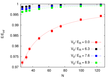
Figure 1: ((Color online) Energy per particle for a system of $N$ particles divided by the same energy in the thermodynamic limit ($N\rightarrow\infty$) as a function of $N$ for different values of the optical potential depth, $V_{z}$, for the case $R$= 1. See further explanation in the text.

What we see in Fig. 1 is that the finite size effects that could affect the energy are greatly reduced when one goes from an homogeneous gas to a gas loaded in an optical lattice. For instance, to use $E_{27}$ as approximation for $E_{\infty}$ for an homogeneous gas has an error of about 3%, while to do the same for any of the $V_{z}$’s considered, reduces that same error an order of magnitude, up to $\sim$ 0.3 %. If we use $E_{64}$ instead, the approximation is true within a 0.1%. That is the reason why in most our calculations we considered simulation cells with a number of potential wells in the range $N$ = 27-64. Moreover, we verified that for $R$ = 1, the critical value of $V_{z}$ obtained from calculations with $3^{3}$, $4^{3}$ and $5^{3}$ simulation cells was the same.

The critical potential depths for the appearance of a Mott insulator phase obtained from our DMC calculations are displayed in Fig. 2, as a function of $R$, as full squares, together with their associated error bars. They were obtained for simulation cells in the range $3^{3}$ ($R>1$) to $4^{3}$ ($R<1$) potential minima. In that figure, for large values of $R$ (the right-hand end), our system can be described as a set quasi-one dimensional tubes, since for $R\rightarrow\infty$, we can write Eq. (1) as:

$$V_{ext}(\vec{r}_{i})=RV_{z}k^{2}(x_{i}^{2}+y_{i}^{2})+V_{z}\sin^{2}(kz_{i})$$

$$=\frac{1}{2}m\omega_{\perp}^{2}(x_{i}^{2}+y_{i}^{2})+V_{z}\sin^{2}(kz_{i}),$$ (5)

simply by developing $\sin(kx_{i})$ and $\sin(ky_{i})$ around $x=0$ and $y=0$. Thus, the critical behavior of these optical lattices is regulated by $V_{z}$, the smallest of the triad $V_{x},V_{y}$ and $V_{z}$. With that in mind, we calculated the critical $V_{z}$ parameters for systems with $R>1$, and displayed them in Fig. 2. Since the optical lattice potential in the perpendicular direction can be approximated in this limit by a Gaussian, we can use the standard deviation of that function, $\sigma_{\perp}=(\hbar/m\omega_{\perp})^{1/2}$, as a measure of the tube ”width”. For our quasi one-dimensional systems, we have:

$$\sigma_{\perp}=\frac{\lambda}{2\pi}\left(\frac{E_{R}}{RV_{z}}\right)^{1/4}$$ (6)

This means that, for $R=100$ and $V_{z}/E_{R}\sim$ 1 (see, Fig. 2), we have $\sigma_{\perp}\sim 2.5a$, a fairly thin tube, considering that the distance between those quasi one-dimensional arrays is $\lambda/2$ = 25$a$. In Fig. (2) we show also (as open circles) the results of Ref. feli3, that can be compared to the ones in this work. Those correspond to quasi-one dimensional Hamiltonians whose optical lattice potentials are defined exactly by Eq. (III), and were obtained using simulation cells with 40 potential minima, which are big enough to be free of finite size effects. The error bars in the $x$ axis for this set of points are derived from the equivalence $\frac{1}{2}m\omega_{\perp}^{2}=RV_{z}k^{2}$, being $V_{z}$ the critical value for the transition in a quasi-one dimensional optical lattice. What we observe is that for $R\geq$ 10, both series of data follow exactly same trend, what implies that even a $3^{3}$ simulation cell is big enough to produce reliable information for this kind of systems. The divergence found for $R\lesssim 3$ probably indicates the breakdown of the approximation given in Eq. III. We also observe that for $1<R<3$ the $V_{z}$ critical values vary smoothly up to the one for a completely symmetric ($R$ = 1) 3D lattice ($V_{z}/E_{R}$ = 8.6 $\pm$ 0.3). This means that critical values for $R$’s other than the ones presented here can be estimated reliably by interpolation between known values. In any case, the comparison of our data with the experiments is straightforward since our results depend on the same magnitudes ($V_{z}$, $E_{R}$, $\lambda$ and $a$).

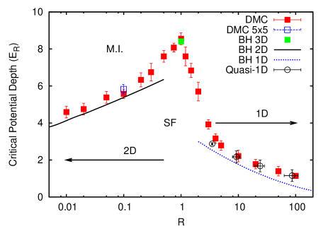
Figure 2: (Color online) Critical value of the optical lattice depth responsible for the superfluid to Mott insulator phase transition (the minimum between $V_{x}$, $V_{y}$ and $V_{z}$) in units of the recoil energy versus $R=V_{x}/V_{z}$. Bose-Hubbard predictions in the limiting cases and quasi-one-dimensional results from Ref. feli3, have been included for comparison.

If we go now to the left-hand side end of Fig. 2 ($R\rightarrow$ 0), we end up with the following approximation to Eq. (1):

$$V_{ext}(\vec{r}_{i})=V_{x}\sin^{2}(k_{x}x_{i})+V_{x}\sin^{2}(k_{y}y_{i})+\frac{V_{x}}{R}\sin^{2}(kz_{i})$$

$$=V_{x}\sin^{2}(k_{x}x_{i})+V_{x}\sin^{2}(k_{y}y_{i})+\frac{1}{2}m\omega_{z}^{2}(z_{i}^{2}),$$ (7)

obtained in the same way as before and taking in mind that now $\frac{V_{x}}{R}$ is very big. Eq. (III) corresponds to a set of quasi two dimensional systems whose critical behavior is regulated by $V_{x}=V_{y}$, the smallest parameter of the triad $V_{x},V_{y},V_{z}$. This value of $V_{x}$ is the one represented in the left-hand side of Fig. 2, not the $V_{z}$ value of the right-hand side already considered above. The limit $R\to 0$ corresponds to a strictly 2D system. The width of the Gaussian in the $z$ direction (the one in which the optical potential can be approximated by an harmonic potential) is:

$$\sigma_{z}=\frac{\lambda}{2\pi}\left(\frac{RE_{R}}{V_{x}}\right)^{1/4},$$ (8)

what implies that for $R$ = 0.01 and $V_{x}/E_{R}\sim$ 4.5, we have $\sigma_{z}\sim$ 1.7$a$, i.e., a set of a very thin quasi two-dimensional ”pancakes”.

In our simulations, we used $3^{3}$ and $4^{3}$ supercells, checking that the results were similar in both cases (full squares), except for $R=0.1$ (open square), for which we represent also the critical $V_{x}$ value for a $5^{2}$ quasi-two dimensional lattice that obeys strictly Eq.(III). Both results are equivalent, i.e., they are not dependent on the geometry of the simulation cell, as in the case $R>1$ discussed above. We can see also a smooth decay in the critical parameter from $R$ = 1 to the smallest $R$ considered ($R=$ 0.01), a behavior similar to the already discussed for the quasi-one dimensional part of the diagram. Unfortunately, we were not able to find in the literature any studies of neutral bosons loaded on quasi two-dimensional systems to compare these results to.

However, they can be compared to the ones given by Bose-Hubbard model. This is a discrete model in which the positions of the particles are limited to the bottom of each potential well. The BH Hamiltonian depends on two parameters, $J$, the hopping matrix element between nearest-neighbor sites, and $U$, related to the interaction between two or more atoms in the same potential well. Both parameters can be obtained from the Hamiltonian in Eq. (2) by approximating the wave function of the system by a combination of Wannier functions corresponding to the lowest energy band jaksch ; cazalilla . In the limit $V_{0}>>E_{R}$, we have

$$\frac{J}{E_{R}}=\frac{4}{\sqrt{\pi}}\left(\frac{V_{0}}{E_{R}}\right)^{\frac{3}{4}}e^{-2\sqrt{\frac{V_{0}}{E_{R}}}}$$ (9)

where $V_{0}$ is the potential depth that determines the critical behavior ($V_{x}$ or $V_{z}$). When, in addition to that approximation, we assumed that the interparticle interaction is described by a pseudopotential, we reach the following expression for $U$:

$$\frac{U}{E_{R}}=\sqrt{\frac{8}{\pi}}ka\left(\frac{V_{x}}{E_{R}}\right)^{\frac{1}{4}}\left(\frac{V_{y}}{E_{R}}\right)^{\frac{1}{4}}\left(\frac{V_{z}}{E_{R}}\right)^{\frac{1}{4}}$$ (10)

Both Eq.(9) and Eq.(10) are approximations, albeit widely used.

From the above equations and the critical values of $U/J$ obtained from exact quantum Monte Carlo calculations found in the literature we can solve for the critical $V_{0}$ value for three-dimensional systems (where $U/J$=29.34, according to 3HD ), two-dimensional ones (with $U/J$=16.739 from2HD ) and one-dimensional optical lattices (where $U/J$ is in the range 3.289-4.651, feli3 ; kuh ). For $R>>1$, this corresponds to the dashed line in Fig. 2, drawn using $(U/J)_{1D}$=3.97, (the center of the interval given above). What we find is that, in general, the BH model underestimates the $V_{z}$ critical, even though when $R>20$ the parameters deduced are closer to our simulation results. In fact, they could be even compatible when we consider all the $(U/J)_{1D}$ values in the literature feli3 . The same can be said of the opposite limit ($R<<1$, full line in Fig. 2): the BH results are always below that of the continuous Hamiltonian, but within the error bars of our data for $R<$ 0.1. On the other hand, the agreement between our $R$ = 1 result and the one derived from a 3D BH model is very good ($V_{z}/E_{R}$ = 8.6 $\pm$ 0.3 versus $(V_{z}/E_{R})_{BH}$ = 8.4), both values being comparable to the experimental one of Ref. mark, ($V_{z}/E_{R}\sim$ 8.8, for a system with $\lambda/a\sim$ 47). Unfortunatelly, the BH model does not seem to describe the behavior in the range 0.2 $<R<$ 3, which is experimentally accessible for different values of $\lambda$. For instance, in Ref. gem, , $R$ is in the range [0.02-1.5]. Another example is the 3D-1D crossover regime of Ref. stoferle, , where the parameter R goes from 1.42 to 5.

IV Conclusions

We have performed DMC calculations that allowed us to calculate the critical potential depths for the appearance of a Mott insulator when the underlying optical lattices were asymmetrical ($V_{x}=V_{y}\neq V_{z}$), a quite common experimental setup. Those results can be compared straightforwardly to those of the experiments, since they depend on the same magnitudes ($V_{x},V_{y},V_{z},\lambda$ and $E_{R}$), and not through indirect variables as the $U$ and $J$’s in the Bose-Hubbard model. In any case, we found that for quasi-one and quasi-two dimensional systems, our results were comparable but larger than the ones deduced from a Bose-Hubbard Hamiltonian. This is the same conclusion as the one found in a similar study for symmetric 3D systems pilati , but extended to quasi one-dimensional and quasi-two dimensional optical lattices.

To be sure, we tested whether the $V_{0}/E_{R}$ critical values deduced from Eqs. (9) and (10), strictly valid when $V_{0}>>E_{R}$, were different when the $J$ and $U$ parameters were calculated numerically from the exact solution of the one-body problem taken from Ref. jaksch, . From those $J$ and $U$, the critical $V_{z}$ parameter for $R=100$ was found to be 0.60$E_{R}$, versus 0.55$E_{R}$ deduced from Eqs. (9) and (10) and the value displayed in Fig. 2. This is still lower than our continuous Hamiltonian result ($V_{z}/E_{R}\sim$ 1). On the other hand, for $R=0.01$, the critical $V_{x}=V_{y}$ estimate was 4.14$E_{R}$, virtually identical to the number displayed in Fig. 2 (4.13$E_{R}$).

All our simulations deal with a single $\lambda/a$ parameter, but a comparison to previous calculations for totally symmetrical systems (Ref. pilati, ) or quasi-one dimensional ones (Ref. feli3, ), indicates that the critical $V_{0}/E_{R}$ values obtained from realistic continuous Hamiltonians are still larger than the ones predicted by the BH model. There is also a rather smooth dependency of the critical value of $V_{0}$ on $\lambda/a$, so in our asymmetrical lattices we would expect a qualitatively similar behavior than the already displayed in Fig. 2. In any case, we think that our results could provide a guide for future experiments in atoms loaded in optical lattices.

- (1) M. Greiner, O. Mandel, T. Esslinger, T.W. Hänsch and I. Bloch. Nature (London) 415 39 (2002).
- (2) I. Bloch. Nat. Phys. 1 23 (2005).
- (3) I. Bloch, J. Dalibard and W. Zwerger Rev. Mod. Phys. 80 885 (2008).
- (4) M. Greiner and S. Fölling. Nature (London) 453 736 (2008).
- (5) I. Bloch, J. Dalibard and S. Nascimbène. Nat. Phys. 8 276 (2012).
- (6) B. Paredes, A. Widera, V. Murg, O. Mandel, S. Fölling, I. Cirac, G.V. Shlyapnikov, T.W. Hänsch and I. Bloch. Nature (London) 429 277 (2004).
- (7) T. Stoferle, H. Moritz, C. Schori, M. Kohl, and T. Esslinger. Phys. Rev. Lett. 92 130403 (2004).
- (8) I. B. Spielman, W. D. Phillips, and J. V. Porto Phys. Rev. Lett. 98 080404 (2007).
- (9) D. Clement, N. Fabbri, L. Fallani, C. Fort, and M. Inguscio. Phys. Rev. Lett. 102 155301 (2009).
- (10) S. Trotzky , L. Pollet, F. Gerbier, U. Schnorrberger, I. Bloch, N. V. Prokof’ev, B. Svistunov, and M. Troyer. Nat. Phys. 6 998 (2010).
- (11) N. Gemelke, X. Zhang, C.L. Hung and C. Ching. Nature (London) 460 995 (2009).
- (12) E. Haller, R. Hart, M.J. Mark, J.G. Danzl, L. Reichsollner, M. Gustavsson, M. Dalmonte, G. Pupillo and H.C. Nagerl. Nature (London). 466 597 (2010).
- (13) M.J. Mark, E. Haller, K. Lauber, J.G. Danzl, A.J. Daley and H.C. Nägerl. Phys. Rev. Lett. 107 175301 (2011).
- (14) H. Imai, T. Akatsuka, T. Ode and A. Morinaga. Phys. Rev. A 85 013633 (2012).
- (15) D. Jaksch, C. Bruder, J.I. Cirac, C.W. Gardiner and P. Zoller. Phys. Rev. Lett. 81 3108 (1998).
- (16) M.A. Cazalilla, R. Citro, T. Giamarchi, E. Orignac and M. Rigol Rev. Mod. Phys. 83,1405 (2011).
- (17) S. Giorgini, J. Boronat and J. Casulleras. Phys. Rev. A 60 5129 (1999).
- (18) M. D. Girardeau, E. M. Wright, and J. M. Triscari. Phys. Rev. A 63 033601 (2001).
- (19) G. E. Astrakharchik and S. Giorgini. Phys. Rev. A 66 053614 (2002).
- (20) D. Blume. Phys. Rev. A 66 053613 (2002).
- (21) S. Pilati, S. Giorgini and N. Prokof’ev. Phys. Rev. Lett. 100 140405 (2008).
- (22) S. Pilati and M. Troyer. Phys. Rev. Lett. 108 155301 (2012).
- (23) F. De Soto and M.C. Gordillo. Phys. Rev. A 85 013607 (2012).
- (24) F. De Soto and M.C. Gordillo. J. Low Temp. Phys. 171 348 (2013).
- (25) C. Carbonell-Coronado, F. De Soto and M.C. Gordillo. Phys. Rev. A 87 063631 (2013).
- (26) J. Boronat and J. Casulleras, Phys. Rev. B 49, 8920 (1994).
- (27) G. G. Batrouni, R.T. Scalettar and G.T. Zimanyi. Phys. Rev. Lett. 65 1765 (1990).
- (28) G. G. Batrouni and R.T. Scalettar. Phys. Rev. B 46 9051 (1992).
- (29) A. Lazarides and M. Haque. Phys. Rev. A 85 063621 (2012).
- (30) H. P. Buchler, G. Blatter, and W. Zwerger. Phys. Rev. Lett. 90 130401 (2003)
- (31) B. Capogrosso-Sansone, N.V. Prokof’ev, and B.V. Svistunov. Phys. Rev. B 75 134302 (2007).
- (32) T.D. Lee, K. Huang, and C.N. Yang, Phys. Rev. 106 1135 (1957).
- (33) T.T. Wu. Phys. Rev. 115 1390 (1959).
- (34) B. Capogrosso-Sansone, S.G. Soyler, N. Prokof’ev and B. Svistunov. Phys. Rev. A 77 015602 (2008).
- (35) T.D. Kühner and H. Monien. Phys. Rev. B Rapid communications 58 R14741 (1998).