Crossover properties of a one-dimensional reaction-diffusion process with a transport current

Abstract

One-dimensional non-equilibrium models of particles subjected to a coagulation-diffusion process are important in understanding non-equilibrium dynamics, and fluctuation-dissipation relation. We consider in this paper transport properties in finite and semi-infinite one-dimensional chains. A set of particles freely hop between nearest-neighbor sites, with the additional condition that, when two particles meet, they merge instantaneously into one particle. A localized source of particle-current is imposed at the origin as well as a non-symmetric hopping rate between the left and right directions (particle drift). This model was previously studied with exact results for the particle density by Hinrichsen et al. [1] in the long-time limit. We are interested here in the crossover process between a scaling regime and long-time behavior, starting with a chain filled of particles. As in the previous reference [1], we employ the empty-interval-particle method, where the probability of finding an empty interval between two given sites is considered. However a different method is developed here to treat the boundary conditions by imposing the continuity and differentiability of the interval probability, which allows for a closed and unique solution, especially for any given initial particle configuration. In the finite size case, we find a crossover between the scaling regime and two different exponential decays for the particle density as function of the input current. Precise asymptotic expressions for the particle-density, and coagulation rate are given.

1 Introduction

Non-equilibrium phenomena in strongly interacting many-body systems often provide complex interactions between fluctuation and dissipation processes, which constitutes an important field of ongoing research [2, 3]. Fluctuations in one dimension are so large that mean field methods are irrelevant, instead exact results are necessary but not always available. One simple model possessing strong fluctuations and critical behavior is represented by the diffusion-coagulation process of indistinguishable particles on a discrete and infinite chain where each site of elementary size $a$ contains at most one particle. The dynamics is defined by particles $A$ that can hop between neighboring sites $A+\O\rightarrow\O+A$ or $\O+A\rightarrow A+\O$ with a rate $\Gamma$ and eventually coagulate $A+A\rightarrow A$ when two particles meet on the same site with probability unity. This model is exactly solvable and the density of particles in the continuum limit, when the product $\Gamma a^{2}=:{\mathscr{D}}$ (diffusion coefficient) is kept constant when $a$ goes to zero, is known to decrease with time like $t^{-1/2}$ (see [4] for a detailed review) in the long-time limit (scaling regime), instead of $t^{-1}$ in the mean-field approximation, implying strong fluctuation effects. Such effects have been observed experimentally, in the kinetics of quasi-particles called excitons on long chains of polymers TMMC=(CH₃)₄N(MnCl₃) [5], and in other types of almost one-dimensional polymers [6, 7]. Interesting quantities such as two-point correlation functions and response functions  [8, 9, 10] can be explicitly evaluated in the continuum limit, invalidating the direct applicability of the fluctuation-dissipation theorem. Introducing external sources is a usual tool to probe the dynamics and influence of time scales in the different transient regimes. Influence of sources was studied in the case of uniform particle deposition with a given constant rate [11, 12, 13] or charge deposition [14] on random chosen sites in one dimensional chains, or even in membranes [15]. In the coagulation-diffusion model, the equation of diffusion for the probability of finding an empty interval of size $x$ is modified by a source term proportional to the size $x$. This equation admits solutions in terms of the Airy function, with eigenvalues proportional to the zeros of this function. It shows interestingly that no first-order rate equation can be written explicitly, except in the asymptotic regime near the stationary state. Relaxation behavior was also studied in the one-dimensional charge aggregation model [16, 14], where particles can coagulate by addition of their charge, and time power law or stretched exponential dependence was found by looking how an excitation charge (or pair of opposite charges) is dissipated into the system using the Green’s function behavior in the long-time regime.

Here we consider the dynamics of a coagulation-diffusion process on a finite and semi-infinite chain with a source of particles at the origin and eventually an asymmetric hopping rate. The aim is to probe the different time scale regimes and steady states, by varying the input current and particle drift, or biased diffusion. Finite size scaling was previously studied in the case of no source term, with open and periodic boundary conditions [17, 18, 19, 1]. Scaling law for the particle concentration $\rho_{L}(t)\simeq L^{-1}F_{0}(8{\mathscr{D}}t/L^{2})$ in a finite chain of size $L$ and diffusion constant ${\mathscr{D}}$ was derived and expressed in particular with Jacobi theta functions, reflecting the Gaussian or diffusive character of the Green’s function. In the following, we consider the possibility of having different crossover regimes in the case of an input current at the origin, which introduces another time scale in the system, or coherent length, after the characteristic time of diffusion through the system $L^{2}/8{\mathscr{D}}$ is reached, and from an initial state where every site is occupied by a single particle.

Such a model was already studied in details with particle inputs and asymmetric diffusion/coagulation rates in reference [1]. The authors were able to extract different asymptotic regimes for the particle density as function of input rate of particles and biased rates in the stationary state. The case with infinite input rate at both ends was also studied previously [20] in relation with the Potts model in one dimension (see also [21]). The analytical treatment presented in this paper is reminiscent of the empty-interval method conveniently used for deriving the exact two-point correlation and response functions [18, 9, 10], in the transient and critical regimes. We can express the average density in the non-stationary regime with a scaling function as $\rho_{L}(t)=L^{-1}F_{0}(8{\mathscr{D}}t/L^{2},k_{in}^{2}L^{2})$, where $k_{in}$ is the typical momentum of the input current $I_{{in}}$ in the continuum limit, expressed as $I_{{in}}=k_{in}^{2}{\mathscr{D}}$. This scaling behavior can be exactly derived from the linear equation of motions for the empty-interval probability. Solving these equations is based on a different method than [1] and is structured as follow: first we write the boundary conditions at both ends of the chain, dependent on the input current, and combine continuity/differentiability relations that include these boundary terms into a general Green’s formalism. Then the continuum limit is derived in part 3, as well as the different transport quantities by using the expression of the empty-interval probability. In parts 5 and 6, we solve the local density in the semi-infinite and finite cases and study the existence of different regimes by identifying the crossover between the scaling regime and the finite size effects at later times, and compute the coagulation rate.

2 Empty interval probability method

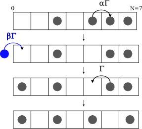
Figure 1: Example of a chain of length $N=7$ filled partially with particles (disks). One time processes occur when particles diffuse to the left or right with rate $\Gamma$ and $\alpha\Gamma$ respectively. Particles can exit the last site on the right with rate $\alpha\Gamma$ and enter from the left with a different rate $\beta\Gamma$ (input current).

We consider a finite one-dimensional chain of $N$ sites filled with particles ($\bullet$) or empty ($\circ$). Particles can diffuse inside the chain with asymmetric rate $\alpha\Gamma$ to the right, with $\alpha\geq 1$, and with rate $\Gamma$ to the left, see Fig. 1. They can also merge (coagulation) on the same site with probability unity. A flux of new particles is introduced from the left hand side of the chain with rate $\beta\Gamma$. Comparing these notations with reference [1], we have the corresponding rates: $a_{L}=c_{L}=\Gamma$, $a_{R}=c_{R}=\alpha\Gamma$ for the biased diffusion $a_{L,R}$ and coagulation $c_{L,R}$ rates, $p_{L}=\beta\Gamma$, and $p_{R}=0$ for the particle inputs on the left and right ends of the chain respectively. The authors also introduced a parameter $q=\sqrt{\alpha}$ which represents the asymmetric diffusion and an input of particles at the origin $p=p_{L}$. We follow the same conditions here and take an initial configuration where the system is full of particles. They were able to compute exact asymptotic regimes for the density:

• In the semi-infinite and discrete case: Exact asymptotic expansions far from the origin as function of finite input rate $p$ and drift ($q$ non equal to 1).

• In the continuum case and semi-infinite system: Exact density expansions far from the origin as function of finite input rate and drift.

• In the continuum case, for infinite input rate $p$, they expressed the density as an exact scaling function of finite ratio $x/L$ in the limit where the system size $L$ and $x$ large (equation 2.62 in their paper). Expansions for $p$ finite (equation 2.65) are also given.

In this paper we use a different scaling regime (time is kept finite, eventually large) and develop a different approach to solve the set of equations of motion by finding appropriate solutions combining the characteristic lengths and time variables into a scaling form. We would like in particular to study in the non-equilibrium state and for any initial condition the transition between massless (for time smaller than the diffusion characteristic time) and massive regimes with the conditions discussed just above.

2.1 Definition of the model and equations of motion in the discrete case

A convenient way to describe in general coagulation-diffusion processes is to introduce the empty-interval probability $E_{n_{1},n_{2}}(t)={\rm Pr}(n_{1}\,\framebox{ d }\,n_{2})$ for $0\leq n_{1}\leq n_{2}\leq N$, $d=n_{2}-n_{1}$ [1], which physically represents the probability to have empty sites at least inside the interval $[n_{1},n_{2}]$ of size $d$. The boundary condition of zero size interval is given by $E_{n_{1},n_{1}}(t)=1$, which is the probability to find no particle. Inside the chain, we can write the following equation of evolution

$$\frac{\partial E_{n_{1},n_{2}}(t)}{\partial t}={\rm Pr}(\stackrel{{\scriptstyle\curvearrowleft}}{{}}n_{1}\,\framebox{$\bullet$ d-1 }\,n_{2})+{\rm Pr}(n_{1}\,\framebox{ d-1 $\bullet$}\,n_{2}\stackrel{{\scriptstyle\curvearrowright}}{{}})$$

$$-{\rm Pr}(\bullet\stackrel{{\scriptstyle\curvearrowright}}{{}}n_{1}\,\framebox{ d }\,n_{2})-{\rm Pr}(n_{1}\,\framebox{ d }\,n_{2}\stackrel{{\scriptstyle\curvearrowleft}}{{}}\bullet).$$ (1)

In this equation, the transition rate ${\rm Pr}(\stackrel{{\scriptstyle\curvearrowleft}}{{}}n_{1}\,\framebox{$\bullet$ d-1 }\,n_{2})$ on the right hand side is the rate at which a particle located in box $[n_{1},n_{1}+1]$ and near an empty interval of size $d-1$ jumps on the left site. It is equal to the product of the rate $\Gamma$ (or $\alpha\Gamma$ if it jumps on the right site) and the probability ${\rm Pr}(n_{1}\,\framebox{$\bullet$d-1 }\,n_{2})$ that such initial configuration exists. The latter probability can be computed using conservative relations and empty interval probabilities as shown below

$${\rm Pr}(\stackrel{{\scriptstyle\curvearrowleft}}{{}}n_{1}\,\framebox{$\bullet$ d-1 }\,n_{2})=\Gamma\times{\rm Pr}(n_{1}\,\framebox{$\bullet$ d-1 }\,n_{2}),$$

$${\rm Pr}(n_{1}\,\framebox{$\bullet$ d-1 }\,n_{2})+{\rm Pr}(n_{1}\,\framebox{$\circ$ d-1 }\,n_{2})={\rm Pr}(n_{1}+1\,\framebox{ d-1 }\,n_{2}),$$

$${\rm Pr}(n_{1}\,\framebox{$\bullet$ d-1 }\,n_{2})=E_{n_{1}+1,n_{2}}-E_{n_{1},n_{2}},$$ (2)

One then obtains, for the dynamics inside the bulk the following equation

$$\frac{\partial E_{n_{1},n_{2}}(t)}{\partial t}=\Gamma\Big{[}E_{n_{1}-1,n_{2}}(t)+E_{n_{1}+1,n_{2}}(t)+E_{n_{1},n_{2}-1}(t)+E_{n_{1},n_{2}+1}(t)$$ (3)

$$-4E_{n_{1},n_{2}}(t)\Big{]}+(\alpha-1)\Gamma\Big{[}E_{n_{1},n_{2}-1}(t)+E_{n_{1}-1,n_{2}}(t)-2E_{n_{1},n_{2}}(t)\Big{]}.$$

The last term in brackets corresponds to the drift contribution $(\alpha-1)\neq 0$ which vanishes when the dynamics is symmetric (no drift term). The first term in brackets is the classic diffusion process in the bulk.

2.2 Boundary conditions

Boundary conditions at locations $n_{1}=0$ and $n_{2}=N$ are found by writing the equations of motion around these points. The treatment of these conditions is done by imposing the continuity and differentiability of the interval probability across the boundaries. We therefore need to determine uniquely the probability functions for all index $n_{1}$ and $n_{2}$ inside and outside the physical domain by extrapolation of the equations of motion. The main advantage is then to use a general Fourier transform which depends only on the initial conditions without introducing Dirichlet conditions. Contrary to reference [1], we do not separate the time from the space dependence, but look at a global solution that combines both time and space variables inside a scaling parameter (see below). This method is similar in some sense to the mirror symmetry method, albeit different, since we are able to construct uniquely the solution for $E$ everywhere by continuity of this function and its derivatives. New particles can enter the left hand side of the chain with rate $\beta\Gamma$ and diffuse through the system with rates $\Gamma$ (left) or $\alpha\Gamma$ (right) before eventually exit the chain on the right with probability $\alpha\Gamma$. We can write (see for example section 2.1 of reference [1])

$$\frac{\partial E_{0,n_{2}}(t)}{\partial t}={\rm Pr}(0\,\framebox{ d-1 $\bullet$}\,n_{2}\stackrel{{\scriptstyle\curvearrowright}}{{}})-{\rm Pr}(0\,\framebox{ d }\,n_{2}\stackrel{{\scriptstyle\curvearrowleft}}{{}}\bullet)-{\rm Pr}(\bullet\stackrel{{\scriptstyle\curvearrowright}}{{}}0\,\framebox{ d }\,n_{2}).$$

The last probability is equal to ${\rm Pr}(\bullet\stackrel{{\scriptstyle\curvearrowright}}{{}}0\,\framebox{ d }\,n_{2})=\beta\Gamma\times{\rm Pr}(0\,\framebox{ d }\,n_{2})=\beta\Gamma E_{0,n_{2}}(t)$ and one obtains

$$\frac{\partial E_{0,n_{2}}(t)}{\partial t}=\Gamma\Big{[}\alpha E_{0,n_{2}-1}(t)+E_{0,n_{2}+1}(t)-(1+\alpha+\beta)E_{0,n_{2}}(t)\Big{]}.$$ (4)

Comparing Eq. (4) with Eq. (3), we can formally extend the first index $n_{1}$ to negative values, by imposing the relation $\alpha E_{-1,n_{2}}(t)+E_{1,n_{2}}(t)=(1+\alpha-\beta)E_{0,n_{2}}(t)$ and which gives a condition of continuity between probabilities with negative index $n_{1}=-1$ and positive one $n_{1}=1$. By differentiating this relation with respect to time, i.e.

$$\alpha\frac{\partial E_{-1,n_{2}}(t)}{\partial t}+\frac{\partial E_{1,n_{2}}(t)}{\partial t}=(1+\alpha-\beta)\frac{\partial E_{0,n_{2}}(t)}{\partial t},$$

and performing some algebra and simplifications involving the two previous identities Eq. (3) and Eq. (4), one obtains formally another relation between quantities $E_{-2,n_{2}}$ and $E_{2,n_{2}}$, assuming that  Eq. (3) holds for all negative locations $-n_{1}$

$$\alpha^{2}E_{-2,n_{2}}(t)+E_{2,n_{2}}(t)=\left[(1+\alpha-\beta)^{2}-2\alpha\right]E_{0,n_{2}}(t).$$ (5)

These two relations obtained for $n_{1}=-1$ and $n_{1}=-2$ are simple enough to suggest a general solution of type

$$\alpha^{n_{1}}E_{-n_{1},n_{2}}(t)+E_{n_{1},n_{2}}(t)={\mathscr{A}}(n_{1})E_{0,n_{2}}(t).$$ (6)

The factor $\alpha^{n_{1}}$ is due to the fact that each time we take the time derivative of Eq. (6), the term $\alpha^{n_{1}}\partial_{t}E_{-n_{1},n_{2}}(t)$ contains the unique contribution from the lowest index $-n_{1}-1$: $\alpha^{n_{1}}\alpha E_{-n_{1}-1,n_{2}}=\alpha^{n_{1}+1}E_{-n_{1}-1,n_{2}}$, and coming from Eq. (4), hence a general factor $\alpha^{n_{1}+1}$ appears. Many terms cancel each other in the further simplifications by taking the time derivative of Eq. (6) for $E_{-n_{1},n_{2}}(t)$ and by assuming recursively that Eq. (6) holds for all $E_{n,n_{2}}$ with $n\leq n_{1}-1$. The initial conditions are given by ${\mathscr{A}}(1)=(1+\alpha-\beta)$ and ${\mathscr{A}}(0)=2$ as found just above for these particular cases. After some algebra, we find that ${\mathscr{A}}(n)$ satisfies the discrete equation ${\mathscr{A}}(n+1)+\alpha{\mathscr{A}}(n-1)={\mathscr{A}}(1){\mathscr{A}}(n)$. The unique solution of this equation is given by

$${\mathscr{A}}(n)=r_{1}^{n}+r_{2}^{n},$$ (7)

with $r_{1}r_{2}=\alpha$ and $r_{1}+r_{2}=1+\alpha-\beta$.

On the right (open) boundary of the chain, we have instead, by counting the different possibilities for particles to create or destroy the empty interval $[n_{1},N]$

$$\frac{\partial E_{n_{1},N}(t)}{\partial t}={\rm Pr}(\stackrel{{\scriptstyle\curvearrowleft}}{{}}n_{1}\,\framebox{$\bullet$ d-1 }\,N)+{\rm Pr}(n_{1}\,\framebox{ d-1 $\bullet$}\,N\stackrel{{\scriptstyle\curvearrowright}}{{}})-{\rm Pr}(\bullet\stackrel{{\scriptstyle\curvearrowright}}{{}}n_{1}\,\framebox{ d }\,N),$$

or, after using the probability relations,

$$\frac{\partial E_{n_{1},N}(t)}{\partial t}=\Gamma\Big{[}\alpha E_{n_{1}-1,N}(t)+E_{n_{1}+1,N}(t)+\alpha E_{n_{1},N-1}(t)-(1+2\alpha)E_{n_{1},N}(t)\Big{]}.$$ (8)

Comparing Eq. (8) with Eq. (3), we can see that the contribution $E_{n_{1},N+1}-E_{n_{1},N}$ is missing, which corresponds to the fact that no particle can enter from the right boundary. Assuming as before that  Eq. (3) is true for $n_{2}\geq N$ by continuity, one obtains the condition $E_{n_{1},N+1}(t)=E_{n_{1},N}(t)$, valid at all time, which gives a first relation for $n_{2}=N+1$. Taking the time derivative of this identity, $\partial_{t}E_{n_{1},N}(t)=\partial_{t}E_{n_{1},N+1}(t)$, using Eq. (3) and the previous relation found for $n_{2}=N+1$, the next relation yields $E_{n_{1},N+2}(t)=(1-\alpha)E_{n_{1},N}(t)+\alpha E_{n_{1},N-1}(t)$. One obtains a relation between $E_{n_{1},N+2}$ and the physical quantities $E_{n_{1},N}$, $E_{n_{1},N-1}$. More generally, by induction, we can try to find a set of coefficients ${\mathscr{B}}(k,l)$ such that $E_{n_{1},N+k}$ depends only on physical quantities $E_{n_{1},N-l}$ for $0\leq l\leq N-k+1$

$$E_{n_{1},N+k}(t)=\sum_{l=0}^{k-1}{\mathscr{B}}(k,l)E_{n_{1},N-l}(t).$$ (9)

A closed form between coefficients ${\mathscr{B}}$ can be found as before by considering the time derivative of Eq. (9) and assuming that Eq. (9) holds from $E_{n_{1},N+1}$ until $E_{n_{1},N+k}$ for a given $k$. We also assume that Eq. (3) holds for all $n_{2}>N$ by continuity. The term $\partial_{t}E_{n_{1},N+k}(t)$ contains the contribution $E_{n_{1},N+k+1}(t)$ which can be expressed as function of $E_{n_{1},N+k}(t)$, $E_{n_{1},N+k-1}(t)$, $\cdots$, $E_{n_{1},N+1}(t)$ and other physical probabilities. Then coefficients ${\mathscr{B}}(k+1,l)$ are function of previous coefficients ${\mathscr{B}}(k^{\prime}\leq k,l^{\prime})$. One obtains after some algebra the discrete recursive equations

$${\mathscr{B}}(k+1,0)={\mathscr{B}}(k,0)+{\mathscr{B}}(k,1)-\alpha{\mathscr{B}}(k-1,0),$$

$${\mathscr{B}}(k+1,l)={\mathscr{B}}(k,l+1)+\alpha{\mathscr{B}}(k,l-1)-\alpha{\mathscr{B}}(k-1,l),\textrm{ for $1\leq l\leq k-2$},$$

$${\mathscr{B}}(k+1,k-1)=\alpha{\mathscr{B}}(k,k-2),\textrm{ and }{\mathscr{B}}(k+1,k)=\alpha{\mathscr{B}}(k,k-1).$$ (10)

By inspection, the boundary conditions are ${\mathscr{B}}(1,0)=1$, ${\mathscr{B}}(k\geq 2,0)=1-\alpha$, and generally ${\mathscr{B}}(k,l)=(1-\alpha)\alpha^{l}$ for other values of $l$, except for the last term ${\mathscr{B}}(k+1,k)=\alpha^{k}$. One obtains the general expression

$$E_{n_{1},N+k}(t)=(1-\alpha)\sum_{l=0}^{k-2}\alpha^{l}E_{n_{1},N-l}(t)+\alpha^{k-1}E_{n_{1},N-k+1}(t).$$ (11)

These continuity equations can be generalized to other boundary conditions, for example when two sources are present at both ends of the chain. In principle one obtains non-local kernel equations relating positive and negative coordinates, such as Eq. (11). The method developed in this paper is quite straightforward, based on the discrete case. However, there is no guarantee that a simple solution can be found in the form of Eq. (9). Moreover, for finite size systems, imposing two sources and an asymmetric diffusion coefficient leads to work with two non-local kernels, which renders the general expression for the interval probability hard to work with, or even to write explicitly as function of the initial conditions.

3 Continuum limit and symmetry equations

In this section we consider the continuum limit of Eq. (3) satisfying the different boundary conditions previously obtained. If $a$ is the elementary lattice step, we introduce coordinates $x_{1}=n_{1}a$ and $x_{2}=n_{2}a$, while $L=Na$ is finite when both $a\rightarrow 0$ and $N\rightarrow\infty$. In this case $E_{n_{1},n_{2}}(t)\rightarrow E(x_{1},x_{2};t)$ and Eq. (3) becomes the equation of diffusion

$$\frac{\partial E(x_{1},x_{2};t)}{\partial t}={\mathscr{D}}\left(\frac{\partial^{2}}{\partial x_{1}^{2}}+\frac{\partial^{2}}{\partial x_{2}^{2}}\right)E(x_{1},x_{2};t)-v\left(\frac{\partial}{\partial x_{1}}+\frac{\partial}{\partial x_{2}}\right)E(x_{1},x_{2};t),$$ (12)

where ${\mathscr{D}}=\Gamma a^{2}$ is the diffusion coefficient in the limit $a\rightarrow 0$ and $\Gamma\rightarrow\infty$, and $v=2k_{b}{\mathscr{D}}$ is the drift velocity, $k_{b}$ being the characteristic momentum from the scaling $\alpha=1+2k_{b}a$ (see Table 1). We can notice that $\alpha\rightarrow 1$ in the continuum limit.

Table 1: Notation and continuum limit for the physical quantities

a	lattice step	L	system size
$\Gamma$	diffusion rate to the left	${\mathscr{D}}=\Gamma a^{2}$	diffusion constant
$\alpha\Gamma$	diffusion rate to the right	$\beta\Gamma$	input rate of particles
$\alpha=1+2k_{b}a$	scaling limit for $\alpha$	$k_{in}=\sqrt{\beta}/a$	input momentum
$v=2k_{b}{\mathscr{D}}$	drift velocity	$l_{0}=\sqrt{8{\mathscr{D}}t}$	diffusion length
$I_{in}={\mathscr{D}}k_{in}^{2}$	input current	$I_{out}(t)=-\frac{{\mathscr{D}}}{2}\partial_{1}^{2}E(L,L;t)$	output current
$\eta_{L}(t)=I_{out}(t)/I_{in}$	current ratio	$\rho(x;t)=\frac{1}{2}(\partial_{1}-\partial_{2})E(x,x;t)$	local particle concentration
$\rho_{L}(t)=L^{-1}\int_{0}^{L}\rho(x;t)\,dx$	averaged concentration	$\Lambda=\sqrt{k_{b}^{2}-k_{in}^{2}}$	effective wavenumber
$t_{L}=L^{2}/8{\mathscr{D}}$	characteristic time	$\epsilon=L^{2}/l_{0}^{2}=t_{L}/t$	inverse time parameter
$R(x;t)$	local coagulation rate	$R(t)$	global coagulation rate
${\cal N}_{L}=\int_{0}^{L}\rho(x;t)dx$	number of particles

Equation (12) is solved using a double Fourier transform $E(x_{1},x_{2};t)=\int_{-\infty}^{+\infty}\int_{-\infty}^{+\infty}\frac{dk_{1}dk_{2}}{4\pi^{2}}\exp({\rm i}k_{1}x_{1}+{\rm i}k_{2}x_{2})\widetilde{E}(k_{1},k_{2};t)$, and the evolution of the empty-interval probability as function of initial conditions is given by

$$E(x_{1},x_{2};t)=\int_{-\infty}^{+\infty}\int_{-\infty}^{+\infty}\!\frac{dx_{1}^{\prime}dx_{2}^{\prime}}{4\pi{\mathscr{D}}t\,}\>\exp\Big{[}-\frac{1}{4{\mathscr{D}}t}(x_{1}-x_{1}^{\prime}-vt)^{2}-\frac{1}{4{\mathscr{D}}t}(x_{2}-x_{2}^{\prime}-vt)^{2}\Big{]}E(x_{1}^{\prime},x_{2}^{\prime};0)$$

$$=\int_{-\infty}^{\infty}\int_{-\infty}^{\infty}\!dx_{1}^{\prime}dx_{2}^{\prime}\>{\mathscr{W}}_{\mbox{\small$l_{0}$}}(\mbox{\small$x_{1}-x_{1}^{\prime}$}){\mathscr{W}}_{\mbox{\small$l_{0}$}}(\mbox{\small$x_{2}-x_{2}^{\prime}$})E(x_{1}^{\prime},x_{2}^{\prime};0),$$

$${\mathscr{W}}_{\mbox{\small$l_{0}$}}(\mbox{\small$x$}):=\!\sqrt{\frac{2}{\pi l_{0}^{2}}}\>\exp\Big{\{}-2(x-vt)^{2}/l_{0}^{2}\Big{\}}.$$ (13)

The integrals over the real axis in the previous expression are unrestricted. We also have introduced the classical diffusion length $l_{0}:=\sqrt{8{\mathscr{D}}t\,}$, which acts as the typical scaling length in the problem . The different physical parameters and their continuous versions are given in Table 1. We now treat the boundary conditions in the continuous limit. On the left hand side of the chain, around the origin, the symmetry Eq. (6) has a continuous solution given by

$$\rme^{2k_{b}x_{1}}E(-x_{1},x_{2};t)+E(x_{1},x_{2};t)={\mathscr{A}}(x_{1})E(0,x_{2};t),$$ (14)

where ${\mathscr{A}}(n)\rightarrow{\mathscr{A}}(x=nL)$ satisfies the differential equation

$${\mathscr{A}}^{\prime\prime}(x)-2k_{b}{\mathscr{A}}^{\prime}(x)+k_{in}^{2}{\mathscr{A}}(x)=0,$$ (15)

with initial conditions ${\mathscr{A}}(0)=2$ and ${\mathscr{A}}^{\prime}(0)=2k_{b}$. This equation is deduced from the discrete recursion for ${\mathscr{A}}(n)$, and from the natural scaling $\beta=a^{2}k_{in}^{2}$ where $k_{in}$ is the input momentum. Indeed, the input current is given by $I_{{in}}=\Gamma\beta$ (see next section) which has the finite value $I_{{in}}={\mathscr{D}}k_{in}^{2}$, by replacing $\beta$ with the corresponding scaling. In particular, the continuous limit of Eq. (6) for intervals incorporating the origin, $\alpha E_{-1,n_{2}}(t)+E_{1,n_{2}}(t)=(1+\alpha-\beta)E_{0,n_{2}}(t)$, is $\partial^{2}_{x_{1}}E(0,x_{2};t)-2k_{b}\partial_{x_{1}}E(0,x_{2};t)=-k_{in}^{2}E(0,x_{2};t)$. We may then identify $k_{in}$ with the inverse of a coherent length inside the chain, in the sense that empty intervals are suppressed by large input currents. Then the solution for Eq. (15) is given by ${\mathscr{A}}(x)=2\exp(k_{b}x)\cosh(x\sqrt{k_{b}^{2}-k_{in}^{2}})$. The $\cosh$ function is transformed into a cosine function when $k_{in}>k_{b}$, or ${\mathscr{A}}(x)=2\exp(k_{b}x)\cos(x\sqrt{k_{in}^{2}-k_{b}^{2}})$. We also have a symmetry equation by exchanging the position variables of the interval [14, 22]

$$E(x_{1},x_{2};t)=2-E(x_{2},x_{1};t),$$ (16)

which holds even in presence of a drift term $v$. The continuum version of the second boundary condition Eq. (11) can be found by noticing that the sum of terms proportional to $(1-\alpha)=-2k_{b}a$ becomes an integral, and coefficients $\alpha^{l}$ with $l\geq 0$, in Eq. (9), have a finite limit ${\mathscr{B}}(x):=\exp(2k_{b}x)$ with $x=la$. Then one obtains

$$E(x_{1},L+x_{2};t)=\exp(2k_{b}x_{2})E(x_{1},L-x_{2};t)-2k_{b}\int_{0}^{x_{2}}dy\exp(2k_{b}y)E(x_{1},L-y;t).$$ (17)

It is useful to define the modified function $\widehat{E}(x_{1},x_{2};t):=\exp[-k_{b}(x_{1}+x_{2})]E(x_{1},x_{2};t)$ in order to simplify the different symmetry relations given by the set of three equations

$$\widehat{E}(x_{1},x_{2};t)+\widehat{E}(-x_{1},x_{2};t)={\widehat{\mathscr{A}}}(x_{1})\widehat{E}(0,x_{2};t),\;{\widehat{\mathscr{A}}}(x_{1}):=2\cosh\Big{(}x_{1}\sqrt{k_{b}^{2}-k_{in}^{2}}\Big{)},\textrm{ (a)}$$

$$\widehat{E}(x_{1},x_{2}+L;t)=\widehat{E}(x_{1},L-x_{2};t)-2k_{b}\int_{0}^{x_{2}}dy\exp[2k_{b}(y-x_{2})]\widehat{E}(x_{1},L-y;t),\textrm{ (b)}$$

$$\widehat{E}(x_{1},x_{2};t)+\widehat{E}(x_{2},x_{1};t)=2\exp[-k_{b}(x_{1}+x_{2})].\textrm{ (c)}$$ (18)

In the following, we will consider two cases, as in [1]. The semi-infinite system with $L=\infty$, where symmetries Eq. (18) reduce to (a) and (c), and the finite system with no drift term $k_{b}=0$. In both cases, the interval probability function can be computed explicitly and for any initial configuration of particles. In the next section, we define the important transport quantities in the continuum limit that are used in the next parts of the paper, such as the particle density as function of space and time.

3.1 Physical quantities

We define the average density and coagulation rate inside the chain. The different notations throughout the text for the physical quantities can be found in Table 1. The local density is noted $\rho_{n}(t)$ (or $\rho(x;t)$ in the continuum limit), and is defined by $a^{-1}{\rm Pr}(n\,\framebox{$\bullet$}\,n+1)$ which is equal to $a^{-1}(1-E_{n,n+1}(t))\simeq-\partial_{2}E(x,x;t)$. Short notation $\partial_{i}$, with $i=1,2$, is meant for partial derivation with respect to component $x_{i}$. Similarly, we can write $\rho_{n}(t)=a^{-1}{\rm Pr}(n-1\,\framebox{$\bullet$}\,n)\simeq\partial_{1}E(x,x;t)$, and therefore, by symmetrization,

$$\rho(x;t)=\frac{1}{2}\Big{(}\partial_{1}-\partial_{2}\Big{)}E(x,x;t).$$ (19)

For systems with translational symmetry, $E(x_{1},x_{2};t)=E(x_{2}-x_{1};t)$, then $\partial_{1}=-\partial_{2}$. In this case, the density is simply equal to $\rho(x;t)=-\partial_{x}E(x=0;t)$ and is site-independent. The current entering the system by unit of time at the origin can be defined as the rate $\Gamma\beta$ times the probability that a particle is not present in the interval $[0,1]$ (if a particle is already present, coagulation will occur)

$$I_{in}=\Gamma\beta\times{\rm Pr}(0\,\framebox{$\circ$}\,1)=\Gamma\beta E_{0,1}(t)\simeq\Gamma\beta={\mathscr{D}}k_{in}^{2}.$$

We also consider the local coagulation rate $R_{n}(t)$ as the number of pairs of particles that coagulate in the box $[n,n+1]$ per unit of time. In terms of probabilities, we can write

$$R_{n}(t) = \Gamma\left[\alpha{\rm Pr}(n-1\framebox{$\bullet\stackrel{{\scriptstyle\curvearrowright}}{{}}\,\bullet$}\,n+1)+{\rm Pr}(n\framebox{$\bullet\stackrel{{\scriptstyle\curvearrowleft}}{{}}\,\bullet$}\,n+2)\right]$$ (20)

$$= \alpha\Gamma\left[1-E_{n-1,n}(t)-E_{n,n+1}(t)+E_{n-1,n+1}(t)\right]$$

$$+ \Gamma\left[1-E_{n,n+1}(t)-E_{n+1,n+2}(t)+E_{n,n+2}\right].$$

Indeed, we need at least two particles in two consecutive sites for coagulation to occur. In the continuum limit $R_{n}(t)\rightarrow R(x;t)$, one obtains

$$R(x;t)=-\frac{1}{2}{\mathscr{D}}\left(\partial_{11}+\partial_{22}+6\partial_{12}\right)E(x,x;t).$$ (21)

We have used the relation $(\partial_{1}+\partial_{2})E(x,x;t)=\partial_{x}E(x,x;t)=0$, deduced from the symmetry property Eq. (16) or constraint $E(x,x;t)=1$. The coagulation rate reduces to $R(x;t)=2{\mathscr{D}}\partial_{11}E(x,x;t)$ in the case of translational symmetry, which corresponds to the curvature of the empty interval probability. In a system of size $L$, we can also define a global coagulation rate $R(t)$, which will be studied in the last section, by considering the terms contributing to the loss and gain of particles, and function of the averaged density. First, we define a dimensionless integrated density ${\cal N}_{L}(t):=L\rho_{L}(t):=\int_{0}^{L}\rho(x;t)\,dx$, incorporating the evolution of the number of particles as function of time. Using the input and output currents $I_{in}$ and $I_{out}(t)$ respectively, one obtains the conservation equation

$$\frac{d{\cal N}_{L}(t)}{dt}=I_{in}-I_{out}(t)-R(t),$$ (22)

where the output current $I_{out}$ at the end of the chain is given by the product of the probability that a particle is present in the box $[N-1,N]$, and the rate $\Gamma$, or explicitly

$$I_{out}(t)=\Gamma\times{\rm Pr}(N-1\,\framebox{$\bullet$}\,N)=\Gamma\times\left[1-E_{N-1,N}(t)\right]\simeq-\frac{{\mathscr{D}}}{2}\partial_{1}^{2}E(L,L;t).$$

We considered in particular the fact that $\partial_{1}E(L,L;t)=0$, resulting from the symmetry $E(L+x_{1},L)=E(L-x_{1},L)$. $R(t)$ can therefore be deduced from Eq. (22) if we know the density.

4 Semi-infinite system

When size $L$ is infinite, symmetries Eq. (18) reduce to (a) and (c) only. Eq. (13) can be decomposed relatively to the origin in four sectors, depending on the sign of the two coordinates

$$E(x_{1},x_{2};t)=\int_{-\infty}^{\infty}\int_{-\infty}^{\infty}\!dx_{1}^{\prime}dx_{2}^{\prime}\>{\widehat{\mathscr{W}}}_{\mbox{\small$l_{0}$}}(\mbox{\small$x_{1},x_{1}^{\prime}$}){\widehat{\mathscr{W}}}_{\mbox{\small$l_{0}$}}(\mbox{\small$x_{2},x_{2}^{\prime}$})\widehat{E}(x_{1}^{\prime},x_{2}^{\prime};0)$$

$$=\int_{0}^{\infty}\int_{0}^{\infty}\!dx_{1}^{\prime}dx_{2}^{\prime}\>\left\{{\widehat{\mathscr{W}}}_{\mbox{\small$l_{0}$}}(\mbox{\small$x_{1},x_{1}^{\prime}$}){\widehat{\mathscr{W}}}_{\mbox{\small$l_{0}$}}(\mbox{\small$x_{2},x_{2}^{\prime}$})\widehat{E}(x_{1}^{\prime},x_{2}^{\prime};0)+{\widehat{\mathscr{W}}}_{\mbox{\small$l_{0}$}}(\mbox{\small$x_{1},-x_{1}^{\prime}$}){\widehat{\mathscr{W}}}_{\mbox{\small$l_{0}$}}(\mbox{\small$x_{2},x_{2}^{\prime}$})\widehat{E}(-x_{1}^{\prime},x_{2}^{\prime};0)\right.$$

$$+\left.{\widehat{\mathscr{W}}}_{\mbox{\small$l_{0}$}}(\mbox{\small$x_{1},x_{1}^{\prime}$}){\widehat{\mathscr{W}}}_{\mbox{\small$l_{0}$}}(\mbox{\small$x_{2},-x_{2}^{\prime}$})\widehat{E}(x_{1}^{\prime},-x_{2}^{\prime};0)+{\widehat{\mathscr{W}}}_{\mbox{\small$l_{0}$}}(\mbox{\small$x_{1},-x_{1}^{\prime}$}){\widehat{\mathscr{W}}}_{\mbox{\small$l_{0}$}}(\mbox{\small$x_{2},-x_{2}^{\prime}$})\widehat{E}(-x_{1}^{\prime},-x_{2}^{\prime};0)\right\},$$ (23)

with the notation ${\widehat{\mathscr{W}}}_{\mbox{\small$l_{0}$}}(\mbox{\small$x,y$}):={\mathscr{W}}_{\mbox{\small$l_{0}$}}(\mbox{\small$x-y$})\exp(k_{b}y)$. From Eq. (18), we can deduce the corresponding values in each of the sectors containing negative coordinates (after dropping the time argument for simplification)

$$\widehat{E}(-x_{1}^{\prime},x_{2}^{\prime})={\widehat{\mathscr{A}}}(x_{1}^{\prime})\widehat{E}(0,x_{2}^{\prime})-\widehat{E}(x_{1}^{\prime},x_{2}^{\prime}),$$

$$\widehat{E}(x_{1}^{\prime},-x_{2}^{\prime})=-{\widehat{\mathscr{A}}}(x_{2}^{\prime})\widehat{E}(0,x_{1}^{\prime})+4\rme^{-k_{b}x_{1}^{\prime}}\cosh(k_{b}x_{2}^{\prime})-\widehat{E}(x_{1}^{\prime},x_{2}^{\prime}),$$

$$\widehat{E}(-x_{1}^{\prime},-x_{2}^{\prime})={\widehat{\mathscr{A}}}(x_{1}^{\prime})\Big{[}2\cosh(k_{b}x_{2}^{\prime})-\widehat{E}(0,x_{2}^{\prime})\Big{]}-{\widehat{\mathscr{A}}}(x_{2}^{\prime})\Big{[}2\cosh(k_{b}x_{1}^{\prime})-\widehat{E}(0,x_{1}^{\prime})\Big{]}$$

$$+4\sinh(k_{b}x_{1}^{\prime})\cosh(k_{b}x_{2}^{\prime})+\widehat{E}(x_{1}^{\prime},x_{2}^{\prime}).$$ (24)

The last equation can be deduced from the first two by performing symmetry operation on the first negative coordinate $-x_{1}^{\prime}\rightarrow x_{1}^{\prime}$, then on the second $-x_{2}^{\prime}\rightarrow x_{2}^{\prime}$. Another relation is also possible, by performing the same symmetry operation on the second coordinate $-x_{2}^{\prime}$ first, then on $-x_{1}^{\prime}$. A prescription is necessary in this case to obtain the correct answer: the final result will be given by taking half the sum of these two operations, yielding the third identity Eq. (24). We then insert these expressions in Eq. (23), and rearrange all terms such that the time dependent interval probability is expressed as a sum of different contributions, function of initial condition $E(x_{1},x_{2};0)$ with $x_{1}<x_{2}$, in addition to those which do not depend on it. One obtains, after some algebra, and using symmetry properties in exchanging the variables of integration $x_{1}^{\prime}\leftrightarrow x_{2}^{\prime}$, the following general expression

$$E(x_{1},x_{2};t)=\int_{0}^{\infty}\int_{0}^{\infty}dx_{1}^{\prime}dx_{2}^{\prime}\left[K(x_{1},x_{1}^{\prime})K(x_{2},x_{2}^{\prime})-K(x_{2},x_{1}^{\prime})K(x_{1},x_{2}^{\prime})\right]E(x_{1}^{\prime},x_{2}^{\prime};0)\theta(x_{2}^{\prime}-x_{1}^{\prime})$$

$$+\int_{0}^{\infty}\int_{0}^{\infty}dx_{1}^{\prime}dx_{2}^{\prime}\>{\widehat{\mathscr{A}}}(x_{1}^{\prime})\left[{\widehat{\mathscr{W}}}_{\mbox{\small$l_{0}$}}(\mbox{\small$x_{1},-x_{1}^{\prime}$})K(x_{2},x_{2}^{\prime})-{\widehat{\mathscr{W}}}_{\mbox{\small$l_{0}$}}(\mbox{\small$x_{2},-x_{1}^{\prime}$})K(x_{1},x_{2}^{\prime})\right]E(0,x_{2}^{\prime};0)$$

$$+1+\int_{0}^{\infty}\int_{0}^{\infty}dx_{1}^{\prime}dx_{2}^{\prime}\>\left[{\mathscr{W}}_{\mbox{\small$l_{0}$}}(\mbox{\small$x_{1}-x_{1}^{\prime}$}){\mathscr{W}}_{\mbox{\small$l_{0}$}}(\mbox{\small$x_{2}+x_{2}^{\prime}$})-{\mathscr{W}}_{\mbox{\small$l_{0}$}}(\mbox{\small$x_{2}-x_{1}^{\prime}$}){\mathscr{W}}_{\mbox{\small$l_{0}$}}(\mbox{\small$x_{1}+x_{2}^{\prime}$})\right]\left[1+\rme^{-2kx_{2}^{\prime}}\right]$$

$$+\left[{\mathscr{W}}_{\mbox{\small$l_{0}$}}(\mbox{\small$x_{1}+x_{1}^{\prime}$}){\mathscr{W}}_{\mbox{\small$l_{0}$}}(\mbox{\small$x_{2}+x_{2}^{\prime}$})-{\mathscr{W}}_{\mbox{\small$l_{0}$}}(\mbox{\small$x_{2}+x_{1}^{\prime}$}){\mathscr{W}}_{\mbox{\small$l_{0}$}}(\mbox{\small$x_{1}+x_{2}^{\prime}$})\right]\rme^{-2k_{b}x_{2}^{\prime}}$$

$$+\int_{0}^{\infty}\int_{0}^{\infty}dx_{1}^{\prime}dx_{2}^{\prime}\>\Big{[}K(x_{2},x^{\prime}_{1})K(x_{1},x^{\prime}_{2})-K(x_{1},x^{\prime}_{1})K(x_{2},x^{\prime}_{2})\Big{]}\theta(x^{\prime}_{2}-x^{\prime}_{1})$$ (25)

$$+\int_{0}^{\infty}\int_{0}^{\infty}dx_{1}^{\prime}dx_{2}^{\prime}\>{\widehat{\mathscr{A}}}(x_{1}^{\prime})\left[{\widehat{\mathscr{W}}}_{\mbox{\small$l_{0}$}}(\mbox{\small$x_{1},-x_{1}^{\prime}$}){\widehat{\mathscr{W}}}_{\mbox{\small$l_{0}$}}(\mbox{\small$x_{2},-x_{2}^{\prime}$})-{\widehat{\mathscr{W}}}_{\mbox{\small$l_{0}$}}(\mbox{\small$x_{2},-x_{1}^{\prime}$}){\widehat{\mathscr{W}}}_{\mbox{\small$l_{0}$}}(\mbox{\small$x_{1},-x_{2}^{\prime}$})\right]2\cosh(k_{b}x_{2}^{\prime}),$$

where $\theta(x)$ is the usual Heaviside function, equal to unity if $x>0$, $\theta(0)=1/2$, and zero otherwise. The kernel $K$ is given by

$$K(x_{1},x_{1}^{\prime}):=\left[{\widehat{\mathscr{W}}}_{\mbox{\small$l_{0}$}}(\mbox{\small$x_{1},x_{1}^{\prime}$})-{\widehat{\mathscr{W}}}_{\mbox{\small$l_{0}$}}(\mbox{\small$x_{1},-x_{1}^{\prime}$})\right]\rme^{-k_{b}x_{1}^{\prime}}.$$ (26)

Eq. (25) is consistent with the fact that $E$ can be expressed generally as $E(x_{1},x_{2})=1+A(x_{1},x_{2})$, where $A$ is an antisymmetric function: $A(x_{1},x_{2})=-A(x_{2},x_{1})$. Equation (25) is also general in the sense that any kind of initial conditions can be implemented. As an application, we consider an initial system entirely filled with particles $E(x_{1},x_{2};0)=0$, which simplifies Eq. (25) since the first two integrals vanish. After some algebra, we find that the concentration is the sum of different contributions

$$\rho(x;t)=\rho_{0}(x,k_{b};t)+\frac{1}{4}\exp\left[(k_{b}-\Lambda)x-k_{in}^{2}{\mathscr{D}}t\right]\Big{\{}(k_{b}-\Lambda)n_{0}(x,k_{b};t)n_{0}(x,\Lambda;t)$$

$$+2\rho_{0}(x,k_{b};t)n_{0}(x,\Lambda;t)-2\rho_{0}(x,\Lambda;t)n_{0}(x,k_{b};t)\Big{\}}+\rho_{1}(x,k_{b};t),$$ (27)

where we introduced the momentum $\Lambda:=\sqrt{k_{b}^{2}-k_{in}^{2}}$. Functions $\rho_{0}$, $n_{0}$, and $\rho_{1}$ are defined by the expressions

$$\rho_{0}(x,k;t):=\frac{1}{\sqrt{\pi{\mathscr{D}}t}}\exp\Big{[}-\frac{(x-2k{\mathscr{D}}t)^{2}}{4{\mathscr{D}}t}\Big{]}-k\rme^{2kx}{\rm erfc}\left(\frac{x+2k{\mathscr{D}}t}{2\sqrt{{\mathscr{D}}t}}\right)$$

$$n_{0}(x,k;t):={\rm erfc}\left(\frac{x-2k{\mathscr{D}}t}{2\sqrt{{\mathscr{D}}t}}\right)+\rme^{2kx}{\rm erfc}\left(\frac{x+2k{\mathscr{D}}t}{2\sqrt{{\mathscr{D}}t}}\right),$$

$$\rho_{1}(x,k;t):=\frac{1}{2\sqrt{2\pi{\mathscr{D}}t}}\left[{\rm erfc}\left(\frac{-x+2k{\mathscr{D}}t}{\sqrt{2{\mathscr{D}}t}}\right)-\rme^{4kx}{\rm erfc}\left(\frac{x+2k{\mathscr{D}}t}{\sqrt{2{\mathscr{D}}t}}\right)\right]$$

$$+\frac{k\rme^{4kx}}{2}{\rm erfc}^{2}\left(\frac{x+2k{\mathscr{D}}t}{2\sqrt{{\mathscr{D}}t}}\right)-\frac{1}{4}\partial_{x}{\cal G}_{k}(x,0){\cal G}_{k}(x,0)$$

$$-\frac{k\rme^{2kx}}{\sqrt{\pi{\mathscr{D}}t}}\int_{0}^{\infty}dy\>\exp\left[-\frac{(x-y-2k{\mathscr{D}}t)^{2}}{4{\mathscr{D}}t}\right]{\rm erfc}\left(\frac{x+y+2k{\mathscr{D}}t}{2\sqrt{{\mathscr{D}}t}}\right).$$ (28)

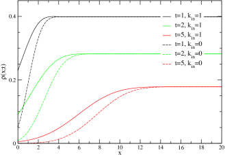
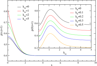
Figure 2: (a) Density profile $\rho(x;t)$ as function of time $t$ in presence of drift $k_{b}=1$ (${\mathscr{D}}=1$). Far from the origin, the density is uniform and equal to $1/\sqrt{2\pi{\mathscr{D}}t}$. (b) Density profile in absence of drift $k_{b}=0$ at time $t=1$ (${\mathscr{D}}=1$) for several $k_{in}$. The density at the origin (inset) is maximum for a finite value of $k_{in}$, function of $k_{b}$. When $k_{in}$ is large, the asymptotic behavior of $\rho(0;t)$ is given by the same value as $k_{in}=0$.

In the last equation, function ${\cal G}_{k}(x,y)$ is given in A, see Eq. (69). When no source and drift are present $k_{b}=k_{in}=0$, the density profile is given by the simple expression

$$\rho(x;t)=\frac{1}{\sqrt{\pi{\mathscr{D}}t}}\exp\left(-\frac{x^{2}}{4{\mathscr{D}}t}\right){\rm erfc}\left(\frac{x}{2\sqrt{{\mathscr{D}}t}}\right)+\frac{1}{\sqrt{2\pi{\mathscr{D}}t}}{\rm erf}\left(\frac{x}{\sqrt{2{\mathscr{D}}t}}\right),$$ (29)

from which we recover the bulk density $\rho(x\gg 1;t)=(2\pi{\mathscr{D}}t)^{-1/2}$ far from the origin. At the origin the density is larger by a factor $\sqrt{2}$: $\rho(x=0;t)=(\pi{\mathscr{D}}t)^{-1/2}$, see Fig. 2(b). In Fig. 2(a) is represented the density profile for a drift momentum $k_{b}=1$ (we set ${\mathscr{D}}=1$), and for several values of time and input momentum $k_{in}$. The density at the origin grows with $k_{in}$ as expected. In Fig. 2(b) we plotted the density profile for several input momenta $k_{in}$ at fixed time and in absence of drift. At the origin, the concentration is given by

$$\rho(0;t)=\rho_{0}(0,k_{b};t)+\exp(-k_{in}^{2}{\mathscr{D}}t)\left[k_{b}-\Lambda+\rho_{0}(0,k_{b};t)-\rho_{0}(0,\Lambda;t)\right].$$ (30)

The density $\rho(0;t)$ is increasing with $k_{in}$ up to a finite value, then decreases as the input current becomes large, see inset of Fig. 2(b). The asymptotic value is equal to the value in absence of current. This feature is characteristic of coagulation-diffusion processes, since coagulation prevents the system to become overpopulated and limits the amount of particles that can be injected into the system. At the same time, diffusion tends to disperse the incoming particles, with the existence of an optimal current $k_{in}\simeq 1$. In the next section, we focus our analysis on the finite size system.

5 Finite system with $k_{b}=0$

Here we consider the case of a system of size $L$, in absence of drift, $k_{b}=0$. In Eq. (13), the integration covers the entire plane ${\mathbb{R}}^{2}$ inside which only the region ${\cal D}_{0}:=\{0\leq x_{1}\leq x_{2}\leq L\}$ is of physical meaning. Symmetries Eq. (18) are used to fold the plane ${\mathbb{R}}^{2}$ into ${\cal D}_{0}$, so that integrations are made only on the physical region given by initial condition $E(x_{1},x_{2};0)$. Equation (13) can be decomposed into sectors of area $L\times L$

$$E(x_{1},x_{2};t)=\int_{0}^{L}\int_{0}^{L}dx_{1}^{\prime}dx_{2}^{\prime}\sum_{m,n=-\infty}^{+\infty}{\mathscr{W}}_{\mbox{\small$l_{0}$}}(\mbox{\small$x_{1}-x_{1}^{\prime}-mL$}){\mathscr{W}}_{\mbox{\small$l_{0}$}}(\mbox{\small$x_{2}-x_{2}^{\prime}-nL$})$$

$$\times E(x_{1}^{\prime}+mL,x_{2}^{\prime}+nL;0).$$ (31)

For example, for $m\geq 0$, we can show recursively the following identities (after dropping the time argument for simplification)

$$E(x_{1}+mL,x_{2})=\left\{\begin{array}[]{rl}(-1)^{p}E(x_{1},x_{2})+\sum_{k=1}^{p}(-1)^{k+1}{\mathscr{A}}([m-2k]L+x_{1})E(0,x_{2})\mbox{, $m=2p$}\\ (-1)^{p}E(L-x_{1},x_{2})+\sum_{k=1}^{p}(-1)^{k+1}{\mathscr{A}}([m-2k]L+x_{1})E(0,x_{2})\mbox{, $m=2p+1$.}\end{array}\right.$$ (34)

We can define the geometric sum $\varphi_{p}(x):=\sum_{k=1}^{p}(-1)^{k+1}{\mathscr{A}}(2[p-k]L+x)$, with the condition $\varphi_{0}(x)=0$, and which can be expressed as

$$\varphi_{p}(x)=\frac{\cos k_{in}[(2p-1)L+x]-(-1)^{p}\cos k_{in}(L-x)}{\cos k_{in}L}.$$ (35)

The previous equation then becomes

$$E(x_{1}+mL,x_{2})=\left\{\begin{array}[]{cl}(-1)^{p}E(x_{1},x_{2})+\varphi_{p}(x_{1})E(0,x_{2})\mbox{, $m=2p$}\\ (-1)^{p}E(L-x_{1},x_{2})+\varphi_{p}(x_{1}+L)E(0,x_{2})\mbox{, $m=2p+1$.}\end{array}\right.$$ (38)

Also, when $m\leq 0$, one obtains after some algebra

$$E(x_{1}+mL,x_{2})=\left\{\begin{array}[]{cl}(-1)^{p}E(x_{1},x_{2})+\varphi_{p}(2L-x_{1})E(0,x_{2})\mbox{, $m=-2p$}\\ (-1)^{p}E(L-x_{1},x_{2})+\varphi_{p}(L-x_{1})E(0,x_{2})\mbox{, $m=-2p+1$.}\end{array}\right.$$ (41)

These expressions can be put into a more compact form such as Eq. (38) with $p$ running from negative to positive values using the symmetry property $\varphi_{-p}(x)=\varphi_{p}(2L-x)$, in which case Eq. (41) is equivalent to Eq. (38) by extrapolation. Equivalently, we also have two different sets of relations for $E(x_{1},x_{2}+nL)$, with $n$ either positive or negative, even or odd. However, we can use the identity $E(x_{1},x_{2}+nL)=2-E(x_{2}+nL,x_{1})$ and Eqs. (38)-(41) to deduce them. It is then sufficient to express $E(x_{1}+2pL,x_{2}+2qL)$ in terms of $E(x_{1},x_{2})$ inside the physical domain ${\cal D}_{0}$. This is done by applying the symmetries on the first argument $x_{1}+2pL\rightarrow x_{1}$, then on the second $x_{2}+2qL\rightarrow x_{2}$, and inversely:

$$E(x_{1}+2pL,x_{2}+2qL)=(-1)^{p+q}E(x_{1},x_{2})-(-1)^{p}\varphi_{q}(x_{2})E(0,x_{1})+(-1)^{q}\varphi_{p}(x_{1})E(0,x_{2})$$

$$+2(-1)^{p}[1-(-1)^{q}]+2\varphi_{p}(x_{1})[1-(-1)^{q}]-\varphi_{p}(x_{1})\varphi_{q}(x_{2})$$ (42)

$$E(x_{1}+2pL,x_{2}+2qL)=(-1)^{p+q}E(x_{1},x_{2})-(-1)^{p}\varphi_{q}(x_{2})E(0,x_{1})+(-1)^{q}\varphi_{p}(x_{1})E(0,x_{2})$$

$$+2[1-(-1)^{q}]-2\varphi_{q}(x_{2})[1-(-1)^{p}]+\varphi_{p}(x_{1})\varphi_{q}(x_{2}).$$ (43)

The result depends therefore on the paths chosen in the plane to map the point $(x_{1}+2pL,x_{2}+2qL)$ onto the physical domain ${\cal D}_{0}$. The correct prescription is to take half the sum of the two previous identities

$$E(x_{1}+2pL,x_{2}+2qL)=(-1)^{p+q}E(x_{1},x_{2})-(-1)^{p}\varphi_{q}(x_{2})E(0,x_{1})+(-1)^{q}\varphi_{p}(x_{1})E(0,x_{2})$$

$$+[1+(-1)^{p}][1-(-1)^{q}]+\varphi_{p}(x_{1})[1-(-1)^{q}]-\varphi_{q}(x_{2})[1-(-1)^{p}].$$ (44)

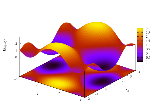
Figure 3: Example of surface $E(x_{1},x_{2})$ after symmetrization for the particular initial conditions $E(x_{1},x_{2}>x_{1};0)=\exp[-\alpha(x_{2}-x_{1})^{2}]$, $\alpha=10$ and $k_{in}=\pi$.

The resulting expression has correct symmetries and continuity. The continuity between domains of size $(L\times L)$ is satisfied using at the boundaries $\varphi_{p+1}(0)=\varphi_{p}(2L)+2(-1)^{p}$. In particular, $E(x_{1},x_{2})$ can be formally written as before as $E(x_{1},x_{2})=1+A(x_{1},x_{2})$ where $A$ is antisymmetric. In Fig. 3 is plotted the resulting surface after symmetrization for a Gaussian distribution $E(x_{1},x_{2}>x_{1};0)$, with an input current, and which satisfies continuous conditions in the entire plane. To obtain the solution for the interval probability at any time, the double sum in Eq. (31) can be further reduced using Eq. (44) for odd and even integers $m$ and $n$,

$$\int_{0}^{L}\int_{0}^{L}dx_{1}^{\prime}\,dx_{2}^{\prime}\sum_{m,n=-\infty}^{+\infty}{\mathscr{W}}_{\mbox{\small$l_{0}$}}(\mbox{\small$x_{1}-x_{1}^{\prime}-mL$}){\mathscr{W}}_{\mbox{\small$l_{0}$}}(\mbox{\small$x_{2}-x_{2}^{\prime}-nL$})E(x_{1}^{\prime}+mL,x_{2}^{\prime}+nL)$$

$$=\int_{0}^{L}\int_{0}^{L}dx_{1}^{\prime}\,dx_{2}^{\prime}\sum_{p,q=-\infty}^{+\infty}\sum_{\epsilon,\epsilon^{\prime}=0,1}{\mathscr{W}}_{\mbox{\small$l_{0}$}}(\mbox{\small$x_{1}-x_{1}^{\prime}-\epsilon L-2pL$}){\mathscr{W}}_{\mbox{\small$l_{0}$}}(\mbox{\small$x_{2}-x_{2}^{\prime}-\epsilon^{\prime}L-2qL$})$$

$$\times E(x_{1}^{\prime}+\epsilon L+2pL,x_{2}^{\prime}+\epsilon^{\prime}L+2qL).$$ (45)

We then replace $E(x_{1}^{\prime}+\epsilon L+2pL,x_{2}^{\prime}+\epsilon^{\prime}L+2qL)$ by its value Eq. (44) in ${\cal D}_{0}$, and the double sum over $(p,q)$ depends explicitly on the two Gaussian series

$$\Psi(x,y):=\sum_{p=-\infty}^{+\infty}{\mathscr{W}}_{\mbox{\small$l_{0}$}}(\mbox{\small$x-y-2pL$})(-1)^{p},\;\chi(x,y):=\sum_{p=-\infty}^{+\infty}{\mathscr{W}}_{\mbox{\small$l_{0}$}}(\mbox{\small$x-y-2pL$})\varphi_{p}(y),$$ (46)

where function $\Psi(x,y)$ is anti-periodic: $\Psi(x,y+2L)=\Psi(x+2L,y)=-\Psi(x,y)$. For example, the first term on the right hand side of Eq. (44) gives

$$\sum_{p,q=-\infty}^{+\infty}{\mathscr{W}}_{\mbox{\small$l_{0}$}}(\mbox{\small$x_{1}-x_{1}^{\prime}-2pL$}){\mathscr{W}}_{\mbox{\small$l_{0}$}}(\mbox{\small$x_{2}-x_{2}^{\prime}-2qL$})(-1)^{p+q}E(x_{1}^{\prime},x_{2}^{\prime})=\Psi(x_{1},x_{1}^{\prime})\Psi(x_{2},x_{2}^{\prime})E(x_{1}^{\prime},x_{2}^{\prime}).$$

The other sums over $(p,q)$ are performed using additional functions $\Psi_{s}(x,y):=\Psi(x,y)-\Psi(x,-y)$ and $\chi_{s}(x,y):=\chi(x,y)+\chi(x,y+L)$, and symmetries $E(L+x_{1}^{\prime},x_{2}^{\prime})=E(L-x_{1}^{\prime},x_{2}^{\prime})$, $E(x_{1}^{\prime},L+x_{2}^{\prime})=E(x_{1}^{\prime},L-x_{2}^{\prime})$. After rearranging the different terms and performing a variable change in the integration over $(x_{1}^{\prime},x_{2}^{\prime})$, one finally obtains

$$E(x_{1},x_{2};t) = 1+G(x_{1})-G(x_{2})-G(x_{1})F(x_{2})+G(x_{2})F(x_{1})+F(x_{1})-F(x_{2})$$ (47)

$$- F(x_{1})F(x_{2})+H(x_{1},x_{2})$$

$$+ G(x_{1})\int_{0}^{L}dx_{2}^{\prime}\Psi_{s}(x_{2},x_{2}^{\prime})E(0,x_{2}^{\prime};0)-G(x_{2})\int_{0}^{L}dx_{1}^{\prime}\Psi_{s}(x_{1},x_{1}^{\prime})E(0,x_{1}^{\prime};0)$$

$$+ \int_{0}^{L}dx_{2}^{\prime}\,\int_{0}^{x_{2}^{\prime}}dx_{1}^{\prime}\left\{\Psi_{s}(x_{1},x_{1}^{\prime})\Psi_{s}(x_{2},x_{2}^{\prime})-\Psi_{s}(x_{2},x_{1}^{\prime})\Psi_{s}(x_{1},x_{2}^{\prime})\right\}E(x_{1}^{\prime},x_{2}^{\prime};0),$$

where we defined the functions

$$F(x):=\int_{0}^{L}\Psi_{s}(x,x^{\prime})\,dx^{\prime},\;G(x):=\int_{0}^{L}\chi_{s}(x,x^{\prime})\,dx^{\prime},$$ (48)

and the contribution coming from the double integral over the two ordered space variables

$$H(x_{1},x_{2}):=2\int_{0}^{L}dx_{1}^{\prime}\Psi_{s}(x_{1},x_{1}^{\prime})\,\int_{0}^{x_{1}^{\prime}}dx_{2}^{\prime}\Psi_{s}(x_{2},x_{2}^{\prime}).$$ (49)

In formula (47), the terms independent of the initial conditions $E(x_{1}^{\prime},x_{2}^{\prime};0)$ in the first two lines contribute to the long time regime. It can be checked again that $E(x_{1},x_{2})=1+A(x_{1},x_{2})$ where $A$ is antisymmetric, and in particular $E(x_{1},x_{1})=1$. In the following we take an initial configuration where particles occupy every site.

5.1 Expression of the density in terms of Elliptic functions

Previous functions $\Psi_{s}$ and $\chi_{s}$ appearing in Eq. (47) can be expressed in terms of Jacobi elliptic functions $\theta_{3}$ and $\theta_{4}$, after performing the sum over the integers in Eq. (46). Similar expressions were found before for the coagulation model with periodic boundary conditions [18]. The details of the computation are given in B and we find

$$\Psi_{s}(x,y)=\sqrt{\frac{2}{\pi l_{0}^{2}}}\left\{\rme^{-\frac{2}{l_{0}^{2}}(x-y)^{2}}\theta_{4}\left(\frac{4iL^{2}}{l_{0}^{2}}\frac{x-y}{L},\rme^{-\frac{8L^{2}}{l_{0}^{2}}}\right)-\rme^{-\frac{2}{l_{0}^{2}}(x+y)^{2}}\theta_{4}\left(\frac{4iL^{2}}{l_{0}^{2}}\frac{x+y}{L},\rme^{-\frac{8L^{2}}{l_{0}^{2}}}\right)\right\},$$

$$\chi_{s}(x,y)=\sqrt{\frac{2}{\pi l_{0}^{2}}}\frac{\rme^{-\frac{2}{l_{0}^{2}}(x-y)^{2}}}{\cos(k_{in}L)}\left\{{\rm Re}\,\left[\rme^{ik_{in}(y-L)}\theta_{3}\left(\frac{4iL^{2}}{l_{0}^{2}}\frac{x-y}{L}-k_{in}L,\rme^{-\frac{8L^{2}}{l_{0}^{2}}}\right)\right]\right.$$

$$-\left.\cos[k_{in}(y-L)]\theta_{4}\left(\frac{4iL^{2}}{l_{0}^{2}}\frac{x-y}{L},\rme^{-\frac{8L^{2}}{l_{0}^{2}}}\right)\right\}+(y\rightarrow y+L).$$ (50)

5.2 Small time behavior

For times $t$ small compare to the characteristic time $t_{L}:=\frac{L^{2}}{8{\mathscr{D}}}$ which is the time for the particles to diffuse through the chain, the ratio $L^{2}/l_{0}^{2}$ is large, and we can replace $\theta_{3}$ and $\theta_{4}$ in Eq. (50) by unity, since the modulus $\exp(-8L^{2}/l_{0}^{2})$ is exponentially small. In this case, one simply obtains

$$\Psi_{s}(x,y)=\sqrt{\frac{2}{\pi l_{0}^{2}}}\left\{\rme^{-\frac{2}{l_{0}^{2}}(x-y)^{2}}-\rme^{-\frac{2}{l_{0}^{2}}(x+y)^{2}}\right\},\;\chi_{s}(x,y)=0.$$ (51)

It is then straightforward to evaluate $F(x)={\rm erf}\left(\sqrt{2}x/l_{0}\right)$ and $G(x)=0$. The local density can be generally expressed in terms of functions $F$, $G$ and $H$ as

$$\rho(x;t)=(1-F(x))G^{\prime}(x)+(1-F(x)+G(x))F^{\prime}(x)+\partial_{1}H(x,x).$$ (52)

Using $\partial_{1}H(x,x)=2\,(\pi l_{0}^{2})^{-1/2}{\rm erf}\left(2x/l_{0}\right)$, we recover Eq. (29) and the system behaves like a system of semi-infinite size without input current. In particular, the integrated density ${\cal N}_{L}(t)$ can be expanded in terms of large parameter $L/l_{0}\gg 1$

$${\cal N}_{L}(t)\simeq\frac{2L}{\sqrt{\pi}l_{0}}+\frac{1}{2}-\frac{1}{\pi}+\left\{\frac{l_{0}}{\sqrt{2\pi}L}-\frac{l_{0}^{3}}{4\sqrt{2\pi}L^{3}}\right\}\exp(-2L^{2}/l_{0}^{2}),$$ (53)

where the first term is the $t^{-1/2}$ law and the corrections are exponentially small in $L^{2}/l_{0}^{2}$.

5.3 Large time expansion

In this section, we analyze the long-time limit of Eq. (50), when $l_{0}\gg L$. In this limit, it is sufficient to study the behavior of the elliptic functions

$$\theta_{3}(z,\exp(-\alpha\epsilon))=1+2\sum_{n=1}^{\infty}\exp(-\alpha\epsilon n^{2})\cos(2nz),$$

$$\theta_{4}(z,\exp(-\alpha\epsilon))=1+2\sum_{n=1}^{\infty}\exp(-\alpha\epsilon n^{2})(-1)^{n}\cos(2nz),$$ (54)

where $\alpha>0$, $z$ complex, and $\epsilon:=L^{2}/l_{0}^{2}$ is the small parameter of the expansion. We can use the Dirac comb identity $\sum_{n=-\infty}^{\infty}\delta(x-n)=\sum_{n=-\infty}^{\infty}\exp(2i\pi nx)$ to rewrite $\theta_{3}(z,\exp(-\alpha\epsilon))$ as

$$\theta_{3}(z,\exp(-\alpha\epsilon))=\int_{-\infty}^{+\infty}dx\sum_{n=-\infty}^{\infty}\delta(x-n)\exp(-\alpha\epsilon x^{2})\cos(2xz)$$

$$=\int_{-\infty}^{+\infty}dx\sum_{n=-\infty}^{\infty}\exp(-\alpha\epsilon x^{2}+2i\pi nx)\cos(2xz)=\sqrt{\frac{\pi}{\alpha\epsilon}}\sum_{n=-\infty}^{\infty}\exp\left[-\frac{1}{\alpha\epsilon}\Big{(}z+n\pi\Big{)}^{2}\right].$$

For $\theta_{4}(z,\exp(-\alpha\epsilon))$, the expression is identical, with instead a shift of $\pm\pi/2$ in the $z$ argument

$$\theta_{4}(z,\exp(-\alpha\epsilon))=\sqrt{\frac{\pi}{\alpha\epsilon}}\sum_{n=-\infty}^{\infty}\exp\left[-\frac{1}{\alpha\epsilon}\Big{(}z+n\pi-\frac{\pi}{2}\Big{)}^{2}\right].$$

Setting $\alpha=8$, $z=4i\epsilon(x-y)/L=:4i\epsilon(u-v)$, with $u:=x/L$ and $v:=y/L$, one obtains the asymptotic limit for the $\theta_{4}$ function in Eq. (50)

$$\theta_{4}(4i\epsilon(u-v),\exp(-8\epsilon))\simeq\sqrt{\frac{\pi}{2\epsilon}}\rme^{-\pi^{2}/32\epsilon+2\epsilon(u-v)^{2}}\cos\left[\frac{\pi}{2}(u-v)\right].$$ (55)

In the case of the $\theta_{3}$ function present in Eq. (50), we take instead $z=4i\epsilon(u-v)-k_{in}L$. The resulting $\theta_{3}$ function is then complex and

$$\theta_{3}(4i\epsilon(u-v)-k_{in}L,\exp(-8\epsilon))\simeq\sqrt{\frac{\pi}{8\epsilon}}\sum_{n=-\infty}^{\infty}\exp\Big{[}-\frac{(n\pi-k_{in}L)^{2}}{8\epsilon}\Big{]}$$

$$\times\exp\Big{[}2\epsilon(u-v)^{2}+i(k_{in}L-n\pi)(u-v)\Big{]}.$$ (56)

Most of the terms in the sum are exponentially small unless $k_{in}L$ is close to $n\pi$ with $n$ integer. Using Eq. (55) and Eq. (56), we can evaluate directly scaling functions $\Psi_{s}(x,y)=:L^{-1}\widetilde{\Psi}_{s}(u,v)$ and $\chi_{s}(x,y)=:L^{-1}\widetilde{\chi}_{s}(u,v)$. In particular, one obtains asymptotically

$$\widetilde{\Psi}_{s}(u,v)\simeq 2\rme^{-\pi^{2}/32\epsilon}\sin\Big{(}\frac{\pi u}{2}\Big{)}\sin\Big{(}\frac{\pi v}{2}\Big{)},$$

$$\widetilde{\chi}_{s}(u,v)\simeq\frac{1}{\cos(k_{in}L)}\left\{-\rme^{-\pi^{2}/32\epsilon}\cos\Big{[}\frac{\pi(u-v)}{2}\Big{]}\cos[k_{in}L(v-1)]\right.$$ (57)

$$+\left.\frac{1}{2}\sum_{n=-\infty}^{\infty}\rme^{-(n\pi-k_{in}L)^{2}/8\epsilon}\cos\Big{[}k_{in}L(v-1)+(k_{in}L-n\pi)(u-v)\Big{]}\right\}+(v\rightarrow v+1).$$

The integration over $v$ can be performed in the previous expansion, $F$ and $G$ are asymptotically given by

$$F(x)\simeq\frac{4}{\pi}\rme^{-\pi^{2}/32\epsilon}\sin\Big{(}\frac{\pi x}{2L}\Big{)}$$

$$G(x)\simeq\rme^{-\pi^{2}/32\epsilon}\frac{\pi}{k_{in}^{2}L^{2}-\pi^{2}/4}\sin\Big{(}\frac{\pi x}{2L}\Big{)}+\rme^{-k_{in}^{2}L^{2}/8\epsilon}\frac{\cos[k_{in}(x-L)]}{\cos(k_{in}L)}.$$ (58)

In the last sum of Eq. (57), only the term $n=0$ does not vanish after integration over variable $v$. Taking into account the dominant terms Eq. (58), and using the fact that $H$ can be approximated by

$$H(x_{1},x_{2})\simeq\frac{16}{\pi^{2}}\rme^{-\pi^{2}/16\epsilon}\sin\Big{(}\frac{\pi x_{1}}{2L}\Big{)}\sin\Big{(}\frac{\pi x_{2}}{2L}\Big{)}=F(x_{1})F(x_{2}),$$ (59)

one obtains for the expression for integrated density ${\cal N}_{L}(t)$, using Eq. (52)

$${\cal N}_{L}(t) = \frac{16k_{in}^{2}L^{2}}{\pi(4k_{in}^{2}L^{2}-\pi^{2})}\rme^{-\pi^{2}t/32t_{L}}+\frac{16\pi k_{in}L\sin(k_{in}L)-16k_{in}^{2}L^{2}-4\pi^{2}}{\pi\cos(k_{in}L)(4k_{in}^{2}L^{2}-\pi^{2})}\rme^{-\left(\pi^{2}+4k_{in}^{2}L^{2}\right)t/32t_{L}}$$ (60)

$$+ \frac{1-\cos(k_{in}L)}{\cos(k_{in}L)}\rme^{-k_{in}^{2}L^{2}t/8t_{L}},$$

where $t_{L}:=L^{2}/8{\mathscr{D}}$ is the diffusion time across the system. In the absence of input current, or $k_{in}=0$, the integrated density simply decreases like ${\cal N}_{L}(t)\simeq 4\pi^{-1}\rme^{-\pi^{2}t/32t_{L}}$.

(a)

(b)

Figure 4: (a) Averaged number of particle ${\cal N}_{L}(t)=L\rho_{L}(t)=\int_{0}^{L}\rho(x;t)\,dx$ as function of time in units of $t_{L}=L^{2}/8{\mathscr{D}}$ (logarithmic scale), for different values of $k_{in}L$. The chain is initially filled with particles. The curves with symbols are the numerical resolution of exact density function using expressions Eq. (50). The red dashed curve for $k_{in}L=0.2$ is the long time behavior Eq. (60), which fits the exact solution for $t>t_{L}$. Black line is the density decay for the scaling regime, $L\gg 1$, given by Eq. (29). (b) Asymptotic regime $l_{0}>L$ or $t>t_{L}$. Magenta dashed line shows the exponential decay $4\pi^{-1}\exp\{-\pi^{2}/32\epsilon\}$ in the limit $k_{in}L=0$, and the black dashed line is the asymptotic fit, Eq. (61), for $k_{in}L=0.5$.

In Fig. 4(a) is represented the evolution of the number of particles ${\cal N}_{L}(t)$ as function of time. For time values less than the diffusion time $t_{L}$, the number decreases like $t^{-1/2}$, and follows closely the result for the bulk Eq. (29). After reaching the diffusion time $t_{L}$, the number decreases exponentially like $\exp(-\pi^{2}t/32t_{L})$, independent of the input current. Then, after a crossover time $t_{c}$, the long-time regime is characterized by the exponential decay ${\cal N}_{L}\sim\exp(-k_{in}^{2}L^{2}t/8t_{L})$ which depends on $k_{in}$. This behavior can be seen explicitly in Fig. 4(b), where the crossover is clearly visible on the averaged number ${\cal N}_{L}(t)$ as function of time (here in units of $t_{L}$) and for different values of $k_{in}L$. After a sharp decreasing behavior dominated mainly by the second term of Eq. (60), the asymptotic regime is accurately given by

$${\cal N}_{L}\simeq\frac{1-\cos(k_{in}L)}{\cos(k_{in}L)}\exp(-k_{in}^{2}L^{2}t/8t_{L}),$$ (61)

which is represented by the black dashed curve for $k_{in}L=0.5$ in Fig. 4(b). The characteristic or relaxation time for this process is actually independent of the system size $L$, and is equal to $8t_{L}/k_{in}^{2}L^{2}=({\mathscr{D}}k_{in}^{2})^{-1}$. The different curves appear to decrease more slowly as $k_{in}L$ is small. The crossover time $t_{c}$ is determined by comparing the second and third terms in Eq. (60), in the limit of small $k_{in}L$ relatively to $\pi/2$:

$$t_{c}=\frac{32t_{L}}{\pi^{2}}\log\left\{\frac{4}{\pi[1-\cos(k_{in}L)]}\right\}.$$ (62)

For example, one obtains $t_{c}/t_{L}\simeq 13$ for $k_{in}L=0.2$, $t_{c}/t_{L}\simeq 18$ for $k_{in}L=0.1$, and $t_{c}/t_{L}\simeq 33$ for $k_{in}L=0.01$, in accordance with data displayed in Fig. 4(a) and (b). We can define a transfer ratio through the finite system as

$$\eta_{L}(t):=I_{out}(t)/I_{in}=-\frac{1}{2}k_{in}^{-2}\partial_{1}^{2}E(L,L;t),$$ (63)

which measures the loss of particles through the system in presence of an input current. From the general expression (47), the current $I_{out}$ and coefficient $\eta_{L}$ can be evaluated with initial conditions where the chain is entirely filled with particles $E(x_{1},x_{2};0)=0$:

$$\eta_{L}(t)=-\frac{1}{2}k_{in}^{-2}\Big{[}\{1-F(L)\}G^{\prime\prime}(L)+\{1+G(L)\}F^{\prime\prime}(L)-F(L)F^{\prime\prime}(L)+\partial_{1}^{2}H(L,L)\Big{]}.$$ (64)

(a)

(b)

Figure 5: (a) Current ratio $\eta_{L}(t)=I_{out}(t)/I_{in}$ as function of time $t$, in units of $t_{L}=L^{2}/8{\mathscr{D}}$, for different values of parameter $k_{in}L$ in the asymptotic regime $t\gg t_{L}$, or when $\epsilon=t_{L}/t$ is small. The current ratio tends to a constant value, around $1/2$ when $k_{in}L$ is small, before decreasing at later times. (b) Current ratio as function of $k_{in}L$ for different time values.

Using approximations (58) and 59), one obtains

$$\eta_{L}(t)=\frac{2\pi}{4k_{in}^{2}L^{2}-\pi^{2}}\rme^{-\pi^{2}t/32t_{L}}-\frac{4k_{in}^{2}L^{2}-\pi^{2}}{2\pi k_{in}^{2}L^{2}\cos(k_{in}L)}\rme^{-\left(\pi^{2}+4k_{in}^{2}L^{2}\right)t/32t_{L}}$$

$$+\frac{1}{2\cos(k_{in}L)}\rme^{-k_{in}^{2}L^{2}t/8t_{L}}.$$ (65)

Figure 5(a) represents $\eta_{L}(t)$ as function of time, in units of $t_{L}$, and for several values of input current $k_{in}L$. We notice first a sharp decreasing of the output current, then a crossover towards a regime with a less pronounced variation. In particular, in the limit of small $k_{in}L\ll 1$, or very low current, $\eta_{L}(t)$ is close to $1/2$. In this limit, one obtains the following expansion

$$\eta_{L}(t)\simeq\frac{1}{2}+\left[\frac{\pi}{2k_{in}^{2}L^{2}}+\frac{\pi}{4}-\frac{4}{\pi}-\frac{\pi t}{16t_{L}}\right]\rme^{-\pi^{2}t/32t_{L}},$$ (66)

for which the value $1/2$ is reached after an interval of time $t_{L}$. Oppositely, figure 5(b) represents the ratio $\eta_{L}(t)$ as function of $k_{in}L$ for different time values. As the size $L$ of the system increases, the ratio goes to zero monotonically as expected. Finally, we can use expressions Eq. (60) and Eq. (65) to compute the coagulation rate $R(t)$, defined by Eq. (22), as function of time. In the long time limit, and for small input current $k_{in}L\ll 1$, the following expansion is obtained

$$R(t)\simeq\frac{1}{2}I_{in}+\frac{\pi}{16t_{L}}\rme^{-\pi^{2}t/32t_{L}}+8I_{in}\rme^{-\pi^{2}t/32t_{L}}\left[\frac{3}{2\pi}-\frac{1}{2}+\frac{\pi}{32}-\frac{\pi t}{128t_{L}}\right],$$ (67)

which shows that half of the input particles coagulate, plus corrective terms which are exponentially small, the last term being negative in this limit. These corrections arise from the finiteness of the system and depend on the time for the input particles to reach the opposite border.

6 Conclusion

In this paper, we presented an application of the empty interval method to the dynamic properties in a reaction-diffusion process, with semi-infinite and finite geometries, as in [1]. The method developed here is well adapted in computing the particle density using only a two-space variable interval probability which satisfies a classical linear equation of diffusion, and which measures specifically the probability of having an empty space between two given sites. The essential point here was to find a different method from [1], to treat the boundary conditions, since there is no possibility to use translation invariance, by incorporating the boundary terms into general symmetries of the probability function. This can be done by extending the problem outside the physical domain, and by introducing a mirror-image like method that takes exactly into account the continuity and differentiability relating negative (unphysical) and positive (physical) interval sizes in the discrete form of the master equation. The effect of a current at the origin, which probes the dynamics for a finite or semi-infinite system, is to induce different time scales, one short time scaling regime, where the density scales like $t^{-1/2}$, and two exponential decays, once the time reaches the typical diffusion time scale through the chain, whose relaxation constant depends on the current value. We were also able to compute the coagulation rate in the asymptotic regime by studying the balance between the different reaction rates. The semi-infinite chain with asymmetry diffusion rate shows also the existence of an optimal current which maximizes the particle density near the origin. This method can also be implemented to treat other boundary conditions and/or initial particle configurations.

Appendix A

Expression of the interval probability function Eq. (25) contains integrals independent of the initial conditions that can be performed exactly, except for the contribution

$$\int_{0}^{\infty}\int_{0}^{\infty}dx_{1}^{\prime}dx_{2}^{\prime}\>\Big{[}K(x_{2},x^{\prime}_{1})K(x_{1},x^{\prime}_{2})-K(x_{1},x^{\prime}_{1})K(x_{2},x^{\prime}_{2})\Big{]}\theta(x^{\prime}_{2}-x^{\prime}_{1})=:{\cal F}_{k}(x_{1},x_{2})-{\cal F}_{k}(x_{2},x_{1}),$$

where function ${\cal F}_{k}$ is given, after performing a first integration, by

$${\cal F}_{k}(x_{1},x_{2})=\int_{0}^{\infty}\frac{dy}{4\sqrt{\pi{\mathscr{D}}t}}\left[\exp\Big{\{}-\frac{(x_{2}-y-2k{\mathscr{D}}t)^{2}}{4{\mathscr{D}}t}\Big{\}}-\rme^{2kx_{2}}\exp\Big{\{}-\frac{(x_{2}+y+2k{\mathscr{D}}t)^{2}}{4{\mathscr{D}}t}\Big{\}}\right]\times$$

$$\left[{\rm erfc}\left(\frac{-x_{1}+y+2k{\mathscr{D}}t}{2\sqrt{{\mathscr{D}}t}}\right)-\rme^{2kx_{1}}{\rm erfc}\left(\frac{x_{1}+y+2k{\mathscr{D}}t}{2\sqrt{{\mathscr{D}}t}}\right)\right].$$ (68)

This integral can be rewritten in a more compact form as

$${\cal F}_{k}(x_{1},x_{2})=-\frac{1}{4}\int_{0}^{\infty}dy\>{\cal G}_{k}(x_{1},y)\partial_{y}{\cal G}_{k}(x_{2},y),$$

$${\cal G}_{k}(x,y):={\rm erfc}\left(\frac{-x+y+2k{\mathscr{D}}t}{2\sqrt{{\mathscr{D}}t}}\right)-\exp\left(2kx\right){\rm erfc}\left(\frac{x+y+2k{\mathscr{D}}t}{2\sqrt{{\mathscr{D}}t}}\right).$$ (69)

After performing one integration by parts, one finds that the contribution $\rho_{1}(x,k;t)$ to the density is given by

$$\rho_{1}(x,k;t)=\left[\partial_{x_{1}}{\cal F}_{k}(x_{1},x_{2})-\partial_{x_{1}}{\cal F}_{k}(x_{2},x_{1})\right]_{x_{1}=x_{2}=x}$$

$$=-\frac{1}{2}\int_{0}^{\infty}dy\>\partial_{x}{\cal G}_{k}(x,y)\partial_{y}{\cal G}_{k}(x,y)-\frac{1}{4}\partial_{x}{\cal G}_{k}(x,0){\cal G}_{k}(x,0).$$ (70)

The integral can be performed partially, leading to ${\rm erf}$ dependent functions in the expression of $\rho_{1}$, Eq. (28).

Appendix B

In this appendix, we propose to express functions $\Psi_{s}(x,y)$ and $\chi_{s}(x,y)$ using elliptic functions. In general, we need to know the explicit expression in terms of elliptic functions of the general Gaussian series $G_{\alpha,\beta}^{\pm}(z)$ defined by

$$G_{\alpha,\beta}^{\pm}(z):=\sum_{n=-\infty}^{+\infty}(\pm 1)^{n}\rme^{-\alpha(z-n)^{2}+2i\beta n},\;\alpha>0.$$ (71)

In particular, these series are complex, with conjugation relation

$$\overline{G_{\alpha,\beta}^{\pm}(z)}=G_{\alpha,\beta}^{\pm}(-z).$$ (72)

We can relate these Gaussian series with the periodic Jacobi elliptic functions $\theta_{3}$ and $\theta_{4}$ which are simply defined by the series expansions

$$\theta_{3}(z,q)=1+2\sum_{n=1}^{\infty}q^{n^{2}}\cos(2nz),\;\theta_{4}(z,q)=1+2\sum_{n=1}^{\infty}(-1)^{n}q^{n^{2}}\cos(2nz)=\theta_{3}(z\pm\frac{\pi}{2},q).$$ (73)

The sum in Eq. (71) can be rearranged such that $G_{\alpha,\beta}^{+}(z)=\rme^{-\alpha z^{2}}\theta_{3}(i\alpha z-\beta,\rme^{-\alpha})$ and $G_{\alpha,\beta}^{-}(z)=\rme^{-\alpha z^{2}}\theta_{4}(i\alpha z-\beta,\rme^{-\alpha})$. In this case, we can rewrite $\Psi_{s}$ as

$$\Psi_{s}(x,y)=\sqrt{\frac{2}{\pi l_{0}^{2}}}\Big{\{}G_{8L^{2}/l_{0}^{2},0}^{-}\Big{(}\frac{x-y}{2L}\Big{)}-G_{8L^{2}/l_{0}^{2},0}^{-}\Big{(}\frac{x+y}{2L}\Big{)}\Big{\}}$$ (74)

$$=\sqrt{\frac{2}{\pi l_{0}^{2}}}\left\{\rme^{-\frac{2}{l_{0}^{2}}(x-y)^{2}}\theta_{4}\left(\frac{4iL^{2}}{l_{0}^{2}}\frac{x-y}{L},\rme^{-\frac{8L^{2}}{l_{0}^{2}}}\right)-\rme^{-\frac{2}{l_{0}^{2}}(x+y)^{2}}\theta_{4}\left(\frac{4iL^{2}}{l_{0}^{2}}\frac{x+y}{L},\rme^{-\frac{8L^{2}}{l_{0}^{2}}}\right)\right\}.$$

For $\chi_{s}(x,y)$, one obtains instead

$$\chi_{s}(x,y)=\sum_{n=-\infty}^{\infty}{\mathscr{W}}_{\mbox{\small$l_{0}$}}(\mbox{\small$x-y-2nL$})\varphi_{n}(y)+{\mathscr{W}}_{\mbox{\small$l_{0}$}}(\mbox{\small$x-y-L-2nL$})\varphi_{n}(y+L)$$ (75)

$$=\sqrt{\frac{2}{\pi l_{0}^{2}}}\frac{1}{\cos(k_{in}L)}{\rm Re}\,\Big{\{}\rme^{ik_{in}(y-L)}G_{8L^{2}/l_{0}^{2},k_{in}L}^{+}\Big{(}\frac{x-y}{2L}\Big{)}-\rme^{ik_{in}(y-L)}G_{8L^{2}/l_{0}^{2},0}^{-}\Big{(}\frac{x-y}{2L}\Big{)}\Big{\}}+(y\rightarrow y+L)$$

$$=\sqrt{\frac{2}{\pi l_{0}^{2}}}\frac{\rme^{-\frac{2}{l_{0}^{2}}(x-y)^{2}}}{\cos(k_{in}L)}{\rm Re}\,\rme^{ik_{in}(y-L)}\left\{\theta_{3}\left(\frac{4iL^{2}}{l_{0}^{2}}\frac{x-y}{L}-k_{in}L,\rme^{-\frac{8L^{2}}{l_{0}^{2}}}\right)\right.$$

$$-\left.\theta_{4}\left(\frac{4iL^{2}}{l_{0}^{2}}\frac{x-y}{L},\rme^{-\frac{8L^{2}}{l_{0}^{2}}}\right)\right\}+(y\rightarrow y+L)$$

$$=\sqrt{\frac{2}{\pi l_{0}^{2}}}\frac{\rme^{-\frac{2}{l_{0}^{2}}(x-y)^{2}}}{\cos(k_{in}L)}\left\{{\rm Re}\,\left[\rme^{ik_{in}(y-L)}\theta_{3}\left(\frac{4iL^{2}}{l_{0}^{2}}\frac{x-y}{L}-k_{in}L,\rme^{-\frac{8L^{2}}{l_{0}^{2}}}\right)\right]\right.$$

$$-\left.\cos[k_{in}(y-L)]\theta_{4}\left(\frac{4iL^{2}}{l_{0}^{2}}\frac{x-y}{L},\rme^{-\frac{8L^{2}}{l_{0}^{2}}}\right)\right\}+(y\rightarrow y+L).$$

References

• [1] Hinrichsen H, Rittenberg V and Simon H 1997 J. Stat. Phys. 86 1203–1235
• [2] ben Avraham D and Havlin S 2000 Diffusion and reactions in fractals and disordered systems (Cambridge University Press)
• [3] Henkel M, Hinrichsen H and Lübeck S 2008 Non-equilibrium phase transitions: absorbing phase transitions vol 1 (Heidelberg: Springer)
• [4] ben Avraham D, Burschka M and Doering C R 1990 J. Stat. Phys. 60 695
• [5] Kroon R, Fleurent H and Sprik R 1993 Phys. Rev. E 47(4) 2462–2472
• [6] Prasad J and Kopelman R 1989 Chem. Phys. Lett. 157 535
• [7] Kopelman R, Li C S and Shi Z Y 1990 J. Luminescence 45 40
• [8] ben Avraham D 1998 Phys. Rev. Lett. 81(21) 4756–4759
• [9] Mayer P and Sollich P 2007 J. Phys. A 40 5823
• [10] Durang X, Fortin J Y and Henkel M 2011 J. Stat. Mech. P02030
• [11] Rácz Z 1985 Phys. Rev. Lett. 55(17) 1707–1710
• [12] Doering C R and ben Avraham D 1989 Phys. Rev. Lett. 62(21) 2563–2566
• [13] Rey P A and Droz M 1997 J. Phys. A: Mathematical and General 30 1101
• [14] Takayasu H, Takayasu M, Provata A and Huber G 1991 J. Stat. Phys. 65 725–745
• [15] Frisch H and Kimball J 1992 Theoretica chimica acta 82 351–356
• [16] Takayasu H 1989 Phys. Rev. Lett. 63(23) 2563–2565
• [17] Alcaraz F, Droz M, Henkel M and Rittenberg V 1994 Ann. of Phys. 230 250
• [18] Krebs K, Pfannmüller M, Wehefritz B and Hinrichsen H 1995 J. Stat. Phys. 78(5) 1429–1470
• [19] Krebs K, Pfannmüller M, Simon H and Wehefritz B 1995 J. Stat. Phys. 78(5) 1471–1491
• [20] Derrida B, Hakim V and Pasquier V 1995 Phys. Rev. Lett. 75(4) 751–754
• [21] Cheng Z, Redner S and Leyvraz F 1989 Phys. Rev. Lett. 62(19) 2321–2324
• [22] Durang X, Fortin J Y, Biondo D D, Henkel M and Richert J 2010 J. Stat. Mech. P04002