Arbitrary-Lagrangian-Eulerian ADER-WENO Finite Volume Schemes with Time-Accurate Local Time Stepping for Hyperbolic Conservation Laws

Abstract

In this article a new high order accurate cell-centered Arbitrary-Lagrangian-Eulerian (ALE) Godunov-type finite volume method with time-accurate local time stepping (LTS) is presented. The method is by construction locally and globally conservative. The scheme is based on a one-step predictor-corrector methodology in space-time and uses three main building blocks: First, a high order piecewise polynomial WENO reconstruction, to obtain a high order data representation in space from the known cell averages of the underlying finite volume scheme. Second, a high order space-time Galerkin predictor step based on a weak formulation of the governing PDE on moving control volumes. Third, a high order one-step finite volume scheme, based directly on the integral formulation of the conservation law in space-time. The algorithm being entirely based on space-time control volumes naturally allows for hanging nodes also in time, hence in this framework the implementation of a consistent and conservative time-accurate LTS becomes very natural and simple. The method is validated on some classical shock tube problems for the Euler equations of compressible gasdynamics and the magnetohydrodynamics equations (MHD). The performance of the new scheme is compared with a classical high order ALE finite volume scheme based on global time stepping. To the knowledge of the author, this is the first high order accurate Lagrangian finite volume method ever presented together with a conservative and time-accurate local time stepping feature.

1 Introduction

After the seminal paper [47] by Munz in 1994, many significant advances have been made in recent years concerning the construction of accurate and robust Godunov-type Lagrangian schemes for hydrodynamics in one and multiple space dimensions, see e.g. the cell-centered Lagrangian finite volume schemes proposed by Maire et al. [46, 44, 43, 45] and Després et al. [14, 8], the staggered Lagrangian scheme presented in [42] or the very recent family of cell-centered ALE remap schemes introduced in [50, 4, 3, 37, 38, 36, 41]. The first better than second order accurate cell-centered Lagrangian finite volume schemes have been proposed by Cheng et al. [10, 39, 11, 12] on structured grids using a nonlinear reconstruction operator of the ENO-type [32], while the first better than second order accurate cell-centered Lagrangian finite volume schemes on unstructured meshes have been recently proposed by Boscheri and Dumbser in [6, 16]. For high order unstructured Lagrangian finite-element schemes the reader is referred to [48, 51] and references therein.

A common shortcoming in all the above mentioned methods is the use of a global time stepping scheme, i.e. the smallest cell usually dictates the timestep of all control volumes in the entire computational domain. Since strong mesh deformation and cell distorsion at shear waves and massive cell clustering at shock waves are common features of all Lagrangian methods, and which naturally also mimick the flow physics on the discrete level, all these methods suffer from very small time steps compared to classical Eulerian finite volume schemes on a fixed mesh, where the mesh quality can be controlled by the user a priori.

In recent years, several successful attempts have been reported in literature to construct high order Eulerian schemes on fixed meshes that allow for time-accurate local time stepping (LTS), where each element can run at its own optimal time step, given by a local CFL stability condition. Most of these schemes were of the discontinuous Galerkin finite element type [28, 20, 53, 40, 29, 35], but also high order accurate finite volume schemes with time accurate LTS can be found, mostly in the context of adaptive mesh refinement (AMR) methods and block-clustered local time-stepping, see [58, 9, 2, 1, 7, 25, 26]. High order Runge-Kutta time integrators with time-accurate local-time stepping have been recently proposed in [31, 30].

In this article, a first attempt is made to introduce time-accurate local time stepping also into high order cell-centered Lagrangian finite volume schemes, in order to reduce the computational effort in the presence of small and highly deformed cells caused by the Lagrangian framework. The paper is organized as follows: in Section 2 the time-accurate local time stepping algorithm is described and all important implementation details are given; in Section 3 some numerical test problems are presented in order to validate the accuracy, efficiency and robustness of the proposed approach; detailed comparisons with global time stepping (GTS) are made; the paper is closed by concluding remarks and an outlook to future extensions in Section 4.

2 Algorithm Description

In this paper, one-dimensional hyperbolic systems of conservation laws of the form

$$\frac{\partial}{\partial t}\mathbf{Q}+\frac{\partial}{\partial x}\mathbf{f}(\mathbf{Q})=0,\qquad x\in\Omega(t)\subset\mathbb{R},\quad t\in\mathbb{R}_{0}^{+},$$ (1)

are considered, where $\mathbf{Q}\in\Omega_{Q}\subset\mathbb{R}^{\nu}$ is the vector of conserved variables and $\mathbf{f}=\mathbf{f}(\mathbf{Q})$ is the nonlinear flux vector. Here, $\Omega(t)$ denotes the time-dependent computational domain and $\Omega_{Q}$ is the set of admissible states, the so-called phase-space or state-space. The computational domain $\Omega(t)$ is discretized by a set of moving mesh points $x_{i+\frac{1}{2}}(t)$, each of which can move with a generic local mesh velocity $V_{i+\frac{1}{2}}(t)$, so that the trajectory of the point satisfies the ODE

$$\frac{d}{dt}x_{i+\frac{1}{2}}=V_{i+\frac{1}{2}}(t).$$ (2)

The Arbitrary-Eulerian-Lagrangian flux vector and its Jacobian are introduced as

$$\mathbf{f}^{V}(\mathbf{Q},V)=\mathbf{f}(\mathbf{Q})-V\mathbf{Q},\qquad\textnormal{ and }\qquad{\mathbf{A}}^{V}(\mathbf{Q},V)=\frac{\partial\mathbf{f}^{V}}{\partial\mathbf{Q}},$$ (3)

where $V$ is the local mesh velocity.

The family of high order one-step cell-centered Lagrangian finite volume schemes described in this section proceeds for each element and (local) time step with the following three subteps:

1. piecewise polynomial data reconstruction from known cell averages, $\mathbf{Q}_{i}^{n}\to\mathbf{w}_{h}(x,t^{n})$,

2. element-local data evolution in time, $\mathbf{w}_{h}(x,t^{n})\to\mathbf{q}_{h}(x,t)$ and

3. one-step element update $\mathbf{Q}_{i}^{n}\to\mathbf{Q}_{i}^{n+1}$ and geometry update $x_{i\pm\frac{1}{2}}^{n}\to x_{i\pm\frac{1}{2}}^{n+1}$.

While this is the natural order of the three steps in the computer program and in the numerical scheme, in the following subsections the three steps of the scheme are described in the opposite order for the sake of clarity, i.e. first the finite volume scheme is presented, then the local data evolution is described and finally the data reconstruction step is outlined.

2.1 One-Step Cell-Centered Lagrangian Finite Volume Scheme with LTS

At time $t$ the spatial control volumes are defined as $T_{i}=T_{i}(t)=[x_{i-\frac{1}{2}}(t);x_{i+\frac{1}{2}}(t)]$. The aim is first to construct a one-step finite volume scheme in space and time, because the use of a one-step time discretization is one of the key ingredients to achieve a simple and efficient local time stepping algorithm. Following [23], the conservation law (1) is first integrated in space and time over a generic space-time control volume $\mathcal{C}_{i}=T_{i}(t)\times[t_{i}^{n};t_{i}^{n+1}]$,

$$\Delta x_{i}^{n+1}\mathbf{Q}_{i}^{n+1}=\Delta x_{i}^{n}\mathbf{Q}_{i}^{n}-\left(\int\limits_{t_{i}^{n}}^{t_{i}^{n+1}}\mathbf{f}^{V}\left(\mathbf{Q}(x_{i+\frac{1}{2}}(t),t),V_{i+\frac{1}{2}}(t)\right)dt-\int\limits_{t_{i}^{n}}^{t_{i}^{n+1}}\mathbf{f}^{V}\left(\mathbf{Q}(x_{i-\frac{1}{2}}(t),t),V_{i-\frac{1}{2}}(t)\right)dt\right).$$ (4)

The integral formulation (4) is by construction locally and globally conservative. If one wants to achieve time-accurate local time stepping (LTS) then a cell $T_{i}$ has to satisfy the so-called update criterion or evolve condition [20, 40]

$$t_{i}^{n}+\Delta t_{i}^{n}\leq\min_{j\in\mathcal{N}_{i}}\left(t_{j}^{n}+\Delta t_{j}^{n}\right),\quad\textnormal{ or equivalently }\quad t_{i}^{n+1}\leq\min_{j\in\mathcal{N}_{i}}\left(t_{j}^{n+1}\right),$$ (5)

where $\mathcal{N}_{i}=\{i-1,i+1\}$ are the side neighbors of $T_{i}$. The current time, the future time and the time step in element $T_{i}$ are denoted by $t_{i}^{n}$, $t_{i}^{n+1}$ and $\Delta t_{i}^{n}$, respectively. Condition (5) means that a cell can be only updated if its future time is less or equal than all the future times of the neighbor elements. Since a time-accurate local time-stepping (LTS) algorithm produces hanging nodes in time at the edges of an element, the flux integrals appearing in (4) are conveniently computed at the aid of a memory variable that properly takes into account all fluxes through the element interfaces $x_{i\pm\frac{1}{2}}$ in the past. The finite volume scheme (4) with LTS then reads

$$\Delta x_{i}^{n+1}\mathbf{Q}_{i}^{n+1}=\Delta x_{i}^{n}\mathbf{Q}_{i}^{n}-\left(\Delta t_{i+\frac{1}{2}}^{n}f^{V}_{i+\frac{1}{2}}-\Delta t_{i-\frac{1}{2}}^{n}f^{V}_{i-\frac{1}{2}}\right)+\mathbf{Q}_{i}^{M}.$$ (6)

In the relations above $\Delta x_{i}(t)=x_{i+\frac{1}{2}}(t)-x_{i-\frac{1}{2}}(t)$ denotes the mesh spacing at a general time $t$. While $\Delta t_{i}^{n}=t_{i}^{n+1}-t_{i}^{n}$ is the size of the current element-local time step the $\Delta t_{i\pm\frac{1}{2}}^{n}$ denote the lengths of the time-intervals on the edges. These edge time-intervals (or flux time-intervals) are defined as

$$\Delta t_{i\pm\frac{1}{2}}^{n}=t_{i\pm\frac{1}{2}}^{n+1}-t_{i\pm\frac{1}{2}}^{n},\quad\textnormal{ with }\left[t_{i\pm\frac{1}{2}}^{n};t_{i\pm\frac{1}{2}}^{n+1}\right]=\left[\max\left(t_{i}^{n},t_{i\pm 1}^{n}\right);\min\left(t_{i}^{n+1},t_{i\pm 1}^{n+1}\right)\right].$$ (7)

For $t_{i}^{n}$ the time step number $n$ is an element-local index and for $t_{i+\frac{1}{2}}^{n}$ it is an edge-local number, but to ease notation we simply always write $n$, intending $n=n(i)$ inside elements and $n=n(i+\frac{1}{2})$ at edges. From (5) and (7) it follows that $t_{i\pm\frac{1}{2}}^{n+1}=t_{i}^{n+1}$. Furthermore, $\Delta x_{i}^{n}=\Delta x_{i}(t_{i}^{n})$ and $\mathbf{Q}_{i}^{n}=\mathbf{Q}_{i}(t_{i}^{n})$. The cell averages are defined as usual as

$$\mathbf{Q}_{i}(t)=\frac{1}{\Delta x_{i}(t)}\int\limits_{x_{i-\frac{1}{2}}(t)}^{x_{i+\frac{1}{2}}(t)}\mathbf{Q}(x,t)dx,$$ (8)

while the time-averaged ALE interface flux across the element boundaries is defined as

$$\mathbf{f}^{V}_{i+\frac{1}{2}}=\frac{1}{\Delta t_{i+\frac{1}{2}}^{n}}\int\limits_{t_{i+\frac{1}{2}}^{n}}^{t_{i+\frac{1}{2}}^{n+1}}\mathbf{f}^{V}\left(\mathbf{Q}(x_{i+\frac{1}{2}}(t),t),V_{i+\frac{1}{2}}(t)\right)\ dt.$$ (9)

In (6) $\mathbf{Q}_{i}^{M}$ is the memory variable [20] that takes into account all fluxes through the element interfaces $x_{i\pm\frac{1}{2}}$ in the past between time $t_{i}^{n}$ and the times $t_{i\pm\frac{1}{2}}^{n}$, i.e.

$$\mathbf{Q}_{i}^{M}=-\left(\int\limits_{t_{i}^{n}}^{t_{i+\frac{1}{2}}^{n}}\mathbf{f}^{V}\left(\mathbf{Q}(x_{i+\frac{1}{2}}(t),t),V_{i+\frac{1}{2}}(t)\right)dt-\int\limits_{t_{i}^{n}}^{t_{i-\frac{1}{2}}^{n}}\mathbf{f}^{V}\left(\mathbf{Q}(x_{i-\frac{1}{2}}(t),t),V_{i-\frac{1}{2}}(t)\right)dt\right).$$ (10)

Using the definition of the memory variable (10) and the LTS finite volume scheme (6) with (9) one obtains again the original integral form of the conservation law (4). In practice, however, the memory variable is not computed directly by formula (10), but according to the following strategy, see also [20]: After a local time-step has been carried out by element $T_{i}$ according to (6), then its memory variable is reset to zero and the fluxes computed through the element interfaces are immediately accumulated into the memory variables of the neighbor cells (to assure conservation), i.e.

$$\mathbf{Q}_{i}^{M}:=0,\qquad\mathbf{Q}_{i\pm 1}^{M}:=\mathbf{Q}_{i\pm 1}^{M}\pm\Delta t_{i\pm\frac{1}{2}}^{n}f^{V}_{i\pm\frac{1}{2}}.$$ (11)

In other words, the flux contributions to the memory variable of a cell $i$ are always computed by the neighbor elements and only the reset step is done by the element itself. It is easy to see that algorithm (11) is equivalent with definition (10), since the time integrals in (10) are additive.

While Eqn. (6) with (8), (9) and (10) is an exact integral relation, a numerical scheme is obtained by using a numerical flux $\mathbf{f}^{V}_{h}(\mathbf{q}_{h}^{-},\mathbf{q}_{h}^{+},V)$ instead of (9), where the flux becomes a function of two state vectors, namely the states $\mathbf{q}_{h}^{-}=\mathbf{q}_{h}(x_{i+\frac{1}{2}}^{-}(t),t)$ and $\mathbf{q}_{h}^{+}=\mathbf{q}_{h}(x_{i+\frac{1}{2}}^{+}(t),t)$ on the left and on the right of the interface, respectively,

$$\mathbf{f}^{V}_{i+\frac{1}{2}}=\frac{1}{\Delta t_{i+\frac{1}{2}}^{n}}\int\limits_{t_{i+\frac{1}{2}}^{n}}^{t_{i+\frac{1}{2}}^{n+1}}\mathbf{f}^{V}_{h}\left(\mathbf{q}_{h}(x_{i+\frac{1}{2}}^{-}(t),t),\mathbf{q}_{h}(x_{i+\frac{1}{2}}^{+}(t),t),V_{i+\frac{1}{2}}(t)\right)dt.$$ (12)

The procedure for the computation of $\mathbf{q}_{h}(x,t)$ will be described in the next section. In this article, two different numerical fluxes are used: either a simple Rusanov-type flux [49], or an Osher-type flux, as introduced in [21, 22]. The Rusanov-type flux reads

$$\mathbf{f}^{V}_{h}(\mathbf{q}_{h}^{-},\mathbf{q}_{h}^{+},V_{i+\frac{1}{2}})=\frac{1}{2}\left(\mathbf{f}^{V}(\mathbf{q}_{h}^{-},V_{i+\frac{1}{2}})+\mathbf{f}^{V}(\mathbf{q}_{h}^{+},V_{i+\frac{1}{2}})\right)-\frac{1}{2}s_{\max}\left(\mathbf{q}_{h}^{+}-\mathbf{q}_{h}^{-}\right),$$ (13)

where $s_{\max}=\max(\max(|\lambda({\mathbf{A}}^{V}(\mathbf{q}_{h}^{-},V_{i+\frac{1}{2}}))|),\max(|\lambda({\mathbf{A}}^{V}(\mathbf{q}_{h}^{+},V_{i+\frac{1}{2}}))|)$ is the maximum signal speed. The Osher-type flux according to [21, 23] reads

$$\mathbf{f}^{V}_{h}(\mathbf{q}_{h}^{-},\mathbf{q}_{h}^{+},V_{i+\frac{1}{2}})=\frac{1}{2}\left(\mathbf{f}^{V}(\mathbf{q}_{h}^{-},V_{i+\frac{1}{2}})+\mathbf{f}^{V}(\mathbf{q}_{h}^{+},V_{i+\frac{1}{2}})\right)-\frac{1}{2}\left(\int\limits_{0}^{1}\left|{\mathbf{A}}^{V}(\mathbf{\Psi}(s),V_{i+\frac{1}{2}})\right|ds\right)\left(\mathbf{q}_{h}^{+}-\mathbf{q}_{h}^{-}\right),$$ (14)

where

$$\mathbf{\Psi}(s)=\mathbf{\Psi}(\mathbf{q}_{h}^{-},\mathbf{q}_{h}^{+},s)=\mathbf{q}_{h}^{-}+s\left(\mathbf{q}_{h}^{+}-\mathbf{q}_{h}^{-}\right)$$ (15)

is a straight-line segment path connecting the two states $\mathbf{q}_{h}^{-}$ and $\mathbf{q}_{h}^{+}$ in phase-space. The integral appearing in Eqn. (14) is computed numerically using Gauss-Legendre quadrature formulae of appropriate order, see [21, 22]. In (14), the usual definition for the absolute value of a matrix ${\mathbf{A}}$ applies:

$$|{\mathbf{A}}|=\mathbf{R}|\mathbf{\Lambda}|\mathbf{R}^{-1},$$ (16)

with $\mathbf{R}$ the matrix of right-eigenvectors and $\mathbf{R}^{-1}$ its inverse, while $|\mathbf{\Lambda}|=\textnormal{diag}(|\lambda_{1}|,|\lambda_{2}|,...,|\lambda_{\nu}|)$ is the diagonal matrix of the absolute values of the eigenvalues of ${\mathbf{A}}$.

For the mesh velocity, needed in (18) and in the fluxes (13) and (14) the Roe averaged velocity for Lagrangian gasdynamics is used, see [47],

$$V_{i+\frac{1}{2}}=\frac{1}{2}\left(V(\mathbf{q}_{h}^{-})+V(\mathbf{q}_{h}^{+})\right),$$ (17)

where $V=V(\mathbf{Q})$ is the local fluid velocity computed from the vector of conserved variables. Note that in Lagrangian gas dynamics, the Roe average for the velocity is simply given by the arithmetic average of the velocities, see [47] for details.

Finally, using (2) and (17), the new positions of the mesh points $x_{i\pm\frac{1}{2}}$ at times $t_{i\pm\frac{1}{2}}^{n+1}$ read

$$x_{i\pm\frac{1}{2}}^{n+1}=x_{i\pm\frac{1}{2}}^{n}+\frac{1}{2}\int\limits_{t_{i\pm\frac{1}{2}}^{n}}^{t_{i\pm\frac{1}{2}}^{n+1}}\left(V(\mathbf{q}_{h}^{-})+V(\mathbf{q}_{h}^{+})\right)dt,$$ (18)

which is the integral form of the ODE (2). For Lagrangian LTS schemes, it is very important to distinguish between the local element times $t_{i}^{n}$ within the space-time element $\mathcal{C}_{i}$ and the local node times $t_{i\pm\frac{1}{2}}^{n}$ at the nodes of the element. Note further that if cell number $i$ is updated, only the meshpoints $x_{i\pm\frac{1}{2}}$ move, the rest of the mesh remains fixed. In other words: if an element $T_{i}$ is updated in time according to (6) it pushes the two nodes that compose element $T_{i}$ according to Eqn. (18).

The integral conservation equation (6) only produces one evolution equation for the cell averages $\mathbf{Q}_{i}(t)$, but since the interface flux $\mathbf{f}^{V}_{i+\frac{1}{2}}$ needs values at the element boundaries, a spatial reconstruction operator is necessary to produce appropriate interface values from the given cell averages. While a first order Godunov finite volume scheme simply uses extrapolation of piecewise constant data to cell boundary $x_{i+\frac{1}{2}}$,

$$\mathbf{q}_{h}^{-}=\mathbf{q}_{h}(x_{i+\frac{1}{2}}^{-},t)=\mathbf{Q}_{i}^{n},\qquad\textnormal{and}\qquad\mathbf{q}_{h}^{+}=\mathbf{q}_{h}(x_{i+\frac{1}{2}}^{+},t)=\mathbf{Q}_{i+1}^{n},$$ (19)

higher order in space can be achieved in the finite volume context by using an appropriate reconstruction or recovery operator. In this paper, a particular form of WENO reconstruction [34] is used, see [23] and Section 2.3.

2.2 High Order Time-Evolution

The high order element-local data evolution stage is another key ingredient for the design of efficient and simple time-accurate local time stepping schemes, see [20, 53, 40, 29]. Instead of the Cauchy-Kovalewski procedure, which is based on cumbersome Taylor series and repeated differentiation of the governing PDE and which has been used in the original ENO method of Harten et al. [32] and in the ADER schemes of Titarev and Toro [54, 55] as well as in the Lagrangian finite volume schemes presented in [39, 12], here a weak integral formulation of the governing PDE in space-time is used. This concept has been introduced in [17, 24, 33], is capable of dealing with stiff algebraic source terms and has already been successfully applied to Lagrangian finite volume schemes with global time stepping (GTS) in [23, 6, 16]. In this section we summarize the description already given in [23], but for the sake of clarity the main steps are explained again to make this article self-contained.

To get an element-local weak formulation of the PDE on a moving space-time control volume $\mathcal{C}_{i}=[x_{i-\frac{1}{2}}(t);x_{i+\frac{1}{2}}(t)]\times[t^{n};t^{n+1}]$, the governing PDE (1) is mapped to the reference space-time element $\mathcal{C}_{E}=[0;1]^{2}$ using an isoparametric mapping, hence the mapping of the geometry is approximated with the same space-time basis functions $\theta_{m}$ that are also used to approximate the discrete solution $\mathbf{q}_{h}(x,t)$. In this paper the $\theta_{m}$ are chosen to be the Lagrange interpolation polynomials of degree $M$ that pass through the tensor-product Gauss-Legendre quadrature points on the reference element $\mathcal{C}_{E}$, see [52] for details on multidimensional quadrature. At the aid of the space-time basis functions $\theta_{k}$, the mapping of $x$ and $t$ onto $\xi$ and $\tau$ reads

$$x_{h}=x(\xi,\tau)=\hat{x}_{m}\theta_{m}(\xi,\tau),\qquad t_{h}=t(\xi,\tau)=\hat{t}_{m}\theta_{m}(\xi,\tau).$$ (20)

Here, $\theta_{m}=\theta_{m}(\xi,\tau)$ and the coefficients $\hat{x}_{m}$ and $\hat{t}_{m}$ denote the nodal coordinates in physical space and time and $\xi$ and $\tau$ are the reference coordinates. A sketch of this isoparametric mapping is depicted in Fig. 1.

Figure 1: Sketch of a third order isoparametric space-time element. Left: physical space-time element. Right: reference space-time element. The interpolation nodes for the numerical solution and for the mapping, given by the tensor-product Gauss-Legendre quadrature points, are numbered from 1 to 9. The initial location for the spatial Gauss-Legendre nodes $\hat{x}_{0,m}$ is also highlighted.

For the time coordinate one gets the following simple mapping, since the time coordinates are the same for each spatial node at each time level:

$$t_{h}=t^{n}+\Delta t_{i}^{n}\tau.$$ (21)

This reduces the Jacobian of the space-time mapping $(\xi,\tau)\to(x,t)$ and its inverse to

$$J=\left(\begin{array}[]{cc}x_{\xi}&x_{\tau}\\ t_{\xi}&t_{\tau}\end{array}\right)=\left(\begin{array}[]{cc}x_{\xi}&x_{\tau}\\ 0&\Delta t_{i}^{n}\end{array}\right),\qquad J^{-1}=\left(\begin{array}[]{cc}\xi_{x}&\xi_{t}\\ \tau_{x}&\tau_{t}\end{array}\right)=\left(\begin{array}[]{cc}\frac{1}{x_{\xi}}&-\frac{1}{\Delta t_{i}^{n}}\frac{x_{\tau}}{x_{\xi}}\\ 0&\frac{1}{\Delta t_{i}^{n}}\end{array}\right).$$ (22)

Using the chain rule PDE (1) is rewritten on the reference element $\mathcal{C}_{E}$ as

$$\frac{\partial\mathbf{Q}}{\partial\tau}-\frac{x_{\tau}}{x_{\xi}}\frac{\partial\mathbf{Q}}{\partial\xi}+\frac{\Delta t_{i}^{n}}{x_{\xi}}\frac{\partial\mathbf{f}}{\partial\xi}=0,$$ (23)

where the second term corresponds to the Lagrangian part of the flux caused by the motion of the mesh. In the framework of isoparametric finite elements, the discrete solution and the flux of PDE (23) are approximated with the same basis functions $\theta_{m}$ used for the mapping (20), i.e.

$$\mathbf{q}_{h}=\mathbf{q}_{h}(\xi,\tau)=\theta_{m}(\xi,\tau)\hat{\mathbf{q}}_{m},\qquad\mathbf{f}_{h}=\mathbf{f}_{h}(\xi,\tau)=\theta_{m}(\xi,\tau)\hat{\mathbf{f}}_{m}.$$ (24)

For a nodal basis, the degrees of freedom of the interpolation of the nonlinear flux are simply computed pointwise as

$$\hat{\mathbf{f}}_{m}=\mathbf{f}(\hat{\mathbf{q}}_{m}).$$ (25)

Throughout the paper, the Einstein summation convention is used. To ease notation, the following operators on $\mathcal{C}_{E}$ are introduced:

$$\left[f,g\right]^{\tau}=\int\limits_{0}^{1}f(\xi,\tau)g(\xi,\tau)\,d\xi,\qquad\textnormal{ and }\qquad\left<f,g\right>=\int\limits_{0^{+}}^{1}\int\limits_{0}^{1}f(\xi,\tau)g(\xi,\tau)\,d\xi\,d\tau.$$ (26)

Multiplication of Eqn. (23) with space-time test functions $\theta_{k}$, integration over $\mathcal{C}_{E}$ and integration of the first term by parts in time yields

$$\left[\theta_{k},\mathbf{q}_{h}\right]^{1}-\left[\theta_{k},\mathbf{w}_{h}\right]^{0}-\left<\frac{\partial}{\partial\tau}\theta_{k},\mathbf{q}_{h}\right>+\left<\theta_{k},\frac{\Delta t_{i}^{n}}{x_{\xi}}\frac{\partial}{\partial\xi}\mathbf{f}_{h}(\mathbf{q}_{h})-\frac{x_{\tau}}{x_{\xi}}\frac{\partial\mathbf{q}_{h}}{\partial\xi}\right>=0.$$ (27)

Here, the initial condition given by the WENO reconstruction polynomial $\mathbf{w}_{h}(x,t^{n})=\psi_{m}(\xi)\hat{\mathbf{w}}_{m}^{n}$ at time $t^{n}$ (see the next sub section) has been introduced in a weak form.

With the definitions for the WENO reconstruction polynomial and the discrete space-time solution (24), one obtains the following element-local nonlinear algebraic equation system:

$$K^{1}_{km}\hat{\mathbf{q}}_{m}+K^{\xi_{x}}_{km}\hat{\mathbf{f}}_{m}-K^{\xi_{t}}_{km}\hat{\mathbf{q}}_{m}=F^{0}_{km}\hat{\mathbf{w}}_{m}^{n},$$ (28)

with

$$K^{1}_{km}=\left(\left<\theta_{k},\frac{\partial}{\partial\tau}\theta_{m}\right>+\left[\theta_{k},\theta_{m}\right]^{0}\right),$$ (29)

$$K^{\xi_{x}}_{km}=\left<\theta_{k},\frac{\Delta t_{i}^{n}}{x_{\xi}}\frac{\partial\theta_{m}}{\partial\xi}\right>,\qquad K^{\xi_{t}}_{km}=\left<\theta_{k},\frac{x_{\tau}}{x_{\xi}}\frac{\partial\theta_{m}}{\partial\xi}\right>,$$ (30)

and

$$F^{0}_{km}=\left[\theta_{k},\psi_{m}\right]^{0},\qquad M_{km}=\left<\theta_{k},\theta_{m}\right>.$$ (31)

The element-local nonlinear algebraic systems (28) can be easily solved using the following iterative method, see [24, 33]:

$$K^{1}_{km}\hat{\mathbf{q}}_{m}^{l+1}+K^{\xi_{x}}_{km}\hat{\mathbf{f}}_{m}^{l}-K^{\xi_{t}}_{km}\hat{\mathbf{q}}_{m}^{l}=F^{0}_{km}\hat{\mathbf{w}}_{m}^{n}.$$ (32)

For an efficient strategy to get the initial guess $\hat{\mathbf{q}}^{0}_{m}$ see [33]. The equation that determines the location of the spatial coordinates $\hat{x}_{m}$ of the space-time element is the ODE

$$\frac{dx}{dt}=V(\mathbf{Q}(x,t)),$$ (33)

where $V(\mathbf{Q}(x,t))$ is the local mesh velocity. For the local mesh velocity one can use again the nodal ansatz

$$V_{h}=V(\mathbf{q}_{h}(x,t))=\theta_{m}(x,t)\hat{v}_{m},\qquad\textnormal{ with }\qquad\hat{v}_{m}=V(\hat{\mathbf{q}}_{m}).$$ (34)

The initial distribution of the spatial Gauss-Legendre quadrature points at time $t_{i}^{n}$ is given by

$$\hat{x}_{0,m}=x_{i-\frac{1}{2}}^{n}+\Delta x_{i}^{n}\zeta_{m},$$ (35)

where the $\zeta_{m}$ are the quadrature points on the unit interval $[0;1]$ and the spatial Lagrange interpolation polynomials passing through these points are denoted by $\phi_{m}$. A discrete version of the ODE (33) can then be obtained using again the local space-time DG method, see [15]:

$$\left([\theta_{k},\theta_{m}]^{1}-\left<\frac{\partial}{\partial\tau}\theta_{k},\theta_{m}\right>\right)\hat{x}^{l+1}_{m}=[\theta_{k},\phi_{m}]^{0}\hat{x}_{0,m}+\Delta t_{i}^{n}\left<\theta_{k},\theta_{m}\right>\hat{v}^{l}_{m}.$$ (36)

The weak formulation for the spatial coordinates (36) is iterated together with the weak formulation for the solution (32) until convergence is reached. The temporal coordinates $\hat{t}_{m}$ are fixed and are given by the Gauss-Legendre points $\zeta_{m}$ in time and relation (21). The space-time polynomials $\mathbf{q}_{h}(x,t)$ are computed for each element in the computational domain and are then used as arguments for the numerical flux in Eqn. (12).

2.3 High Order WENO Reconstruction for LTS

In this paper the polynomial WENO reconstruction algorithm proposed in [18, 19, 17] is used. Its output are reconstruction polynomials and not point values, as in the original optimal WENO scheme of Jiang and Shu [34]. The details can be found in the above-mentioned references, hence only a brief summary of the algorithm is given here together with the necessary modifications in order to support LTS. For the sake of simplicity, componentwise reconstruction in conservative variables is assumed. For reconstruction in characteristic variables see [32, 34]. A reconstruction polynomial $\mathbf{w}_{h}(x,t_{i}^{n})$ of degree $M$ is obtained componentwise by requiring integral conservation on a stencil

$$\mathcal{S}_{i}^{s}=\bigcup\limits_{j=i-l}^{i+r}T_{j}^{n}$$ (37)

with spatial extension $l$ and $r$ to the left and right, respectively. For odd order schemes there is one central stencil ($s=1$), with $l=r=M/2$, while for even order schemes there are two central stencils with $l=$floor$(M/2)+1$ and $r=$floor$(M/2)$ for the first central stencil ($s=0$) and $l=$floor$(M/2)$, $r=$floor$(M/2)+1$ for the second one ($s=1$). All schemes have one fully left-sided stencil ($s=2$) with $l=M$ and $r=0$ and one fully right-sided stencil ($s=3$) with $l=0$ and $r=M$. The reconstruction polynomial for each stencil is written in terms of some spatial basis functions $\psi_{m}(\xi)$ as

$$\mathbf{w}^{s}_{h}(x,t^{n})=\sum\limits_{m=0}^{M}\psi_{m}(\xi)\hat{\mathbf{w}}^{s}_{m}:=\psi_{m}(\xi)\hat{\mathbf{w}}^{n,s}_{m},$$ (38)

with the mapping

$$x=x_{i-\frac{1}{2}}^{n}+\Delta x_{i}^{n}\xi.$$ (39)

For the reconstruction basis functions $\psi_{m}(\xi)$ one can either use Legendre polynomials rescaled to the unit interval $[0;1]$, or, a nodal basis based on the Lagrangian interpolation polynomials passing through the Gauss-Legendre quadrature points on the unit interval. To obtain the high order reconstruction polynomial one usually requires integral conservation on all elements of the stencil as follows:

$$\frac{1}{\Delta x^{n}_{j}}\int\limits_{x^{n}_{j-\frac{1}{2}}}^{x^{n}_{j+\frac{1}{2}}}\mathbf{w}^{s}_{h}(x,t_{i}^{n})dx=\mathbf{Q}^{n}_{j},\qquad\forall T_{j}^{n}\in\mathcal{S}_{i}^{s}.$$ (40)

However, in the context of finite volume schemes with time-accurate local time stepping, each cell average $\mathbf{Q}^{n}_{j}$ is usually defined at a different local time $t_{j}^{n}\neq t_{i}^{n}$, i.e. Eqn. (40) can in general not be used for reconstruction, since the cell averages needed for reconstruction are in general not available at the time $t_{i}^{n}$ when they are needed. Also the geometry of the stencil is in general not available at the time $t_{i}^{n}$ required for reconstruction. Instead, one has to use the following set of reconstruction equations, which uses the local predictor solution $\mathbf{q}_{h}$ in all elements $T_{j}^{n}$ with $j\neq i$ in order to predict the value of the cell averages and the geometry at the required reconstruction time $t_{i}^{n}$. These estimated values are distinguished from the real cell averages and interface positions by the use of the tilde symbol:

$$\frac{1}{\Delta\tilde{x}^{n}_{j}}\int\limits_{\tilde{x}_{j-\frac{1}{2}}(t_{i}^{n})}^{\tilde{x}_{j+\frac{1}{2}}(t_{i}^{n})}\mathbf{w}^{s}_{h}(x,t_{i}^{n})dx=\tilde{\mathbf{Q}}_{j}(t_{i}^{n}),\qquad\forall T_{j}^{n}\in\mathcal{S}_{i}^{s},$$ (41)

with $\Delta\tilde{x}^{n}_{j}=\Delta\tilde{x}_{j}(t_{i}^{n})=\tilde{x}_{j+\frac{1}{2}}(t_{i}^{n})-\tilde{x}_{j-\frac{1}{2}}(t_{i}^{n})$ and

$$\tilde{\mathbf{Q}}_{j}(t_{i}^{n})=\left\{\begin{array}[]{lll}\mathbf{Q}^{n}_{i},&\textnormal{ if }&i=j,\\ \frac{1}{\Delta\tilde{x}^{n}_{j}}\displaystyle\int\limits_{\tilde{x}_{j-\frac{1}{2}}(t_{i}^{n})}^{\tilde{x}_{j+\frac{1}{2}}(t_{i}^{n})}\mathbf{q}_{h}(x,t_{i}^{n})dx,&\textnormal{ if }&i\neq j.\end{array}\right.$$ (42)

The geometry at the reconstruction time $t_{i}^{n}$ is estimated by moving the interfaces virtually, just for the purpose of reconstruction, as follows:

$$\tilde{x}_{j+\frac{1}{2}}(t_{i}^{n})=x_{j+\frac{1}{2}}(t_{j+\frac{1}{2}}^{n})+\int\limits_{t_{j+\frac{1}{2}}^{n}}^{t_{i}^{n}}V_{j+\frac{1}{2}}(t)dt,$$ (43)

where $V_{j+\frac{1}{2}}(t)=\frac{1}{2}\left(V(\mathbf{q}_{h}(x_{j+\frac{1}{2}}^{-}(t),t))+V(\mathbf{q}_{h}(x_{j+\frac{1}{2}}^{+}(t),t))\right)$ is again easily computed using the local predictor $\mathbf{q}_{h}$. Now, the reconstruction equations (41) are defined and the unknown coefficients $\mathbf{w}^{n,s}_{m}$ can be obtained, using the virtual interface positions $\tilde{x}_{j+\frac{1}{2}}(t_{i}^{n})$ and the virtual cell averages $\tilde{\mathbf{Q}}^{n}_{j}$ at the reconstruction time $t_{i}^{n}$, computed from the element-local space-time predictor solution $\mathbf{q}_{h}(x,t)$. As the reader can easily appreciate, it is indeed the use of the predictor-corrector philosophy which allows a simple reconstruction procedure with time-accurate local time-stepping, since the local space-time predictor $\mathbf{q}_{h}$ provides an accurate interpolation of the data and the geometry at any desired position in space and time. From (43) and (42) it becomes clear that an element can only apply the reconstruction operator if the following condition is satisfied:

$$\max(t_{j}^{n})\leq t_{i}^{n}\leq\min(t_{j}^{n+1}),\qquad\forall T_{j}^{n}\in\mathcal{S}_{i}^{s},$$ (44)

i.e. the reconstruction time $t_{i}^{n}$ must be contained within all local time intervals $[t_{j}^{n};t_{j}^{n+1}]$ of all stencil elements so that the local predictor solution can be evaluated at a valid relative time $0\leq\tau\leq 1$. The predictor is not valid for $\tau<0$ (backward extrapolation in time) or $\tau>1$ (forward extrapolation in time). Note that for better than second order schemes condition (44) is more restrictive than the simple update criterion (5), hence from third order methods onward one has to obey condition (44).

With the oscillation indicators $\sigma_{s}$

$$\sigma_{s}=\Sigma_{lm}\hat{\mathbf{w}}^{n,s}_{l}\hat{\mathbf{w}}^{n,s}_{m},\qquad\Sigma_{lm}=\sum\limits_{\alpha=1}^{M}\int\limits_{0}^{1}\frac{\partial^{\alpha}\psi_{l}(\xi)}{\partial\xi^{\alpha}}\cdot\frac{\partial^{\alpha}\psi_{m}(\xi)}{\partial\xi^{\alpha}}d\xi,$$ (45)

the nonlinear weights $\omega_{s}$ are defined by

$$\tilde{\omega}_{s}=\frac{\lambda_{s}}{\left(\sigma_{s}+\epsilon\right)^{r}},\qquad\omega_{s}=\frac{\tilde{\omega}_{s}}{\sum_{q}\tilde{\omega}_{q}},$$ (46)

where we use $\epsilon=10^{-14}$, $r=8$, $\lambda_{s}=1$ for the one-sided stencils and $\lambda=10^{5}$ for the central stencils, according to [17, 18]. The final nonlinear WENO reconstruction polynomial and its coefficients are then given by

$$\mathbf{w}_{h}(x,t^{n})=\psi_{m}(\xi)\hat{\mathbf{w}}^{n}_{m},\qquad\textnormal{ with }\qquad\hat{\mathbf{w}}^{n}_{m}=\sum_{s}\omega_{s}\hat{\mathbf{w}}^{n,s}_{m}.$$ (47)

For the computation of the time step $\Delta t_{i}$, each element obeys the following local CFL condition

$$\Delta t_{i}^{n}=\textnormal{CFL}\cdot\min_{j\in\mathcal{N}_{i}}\left(\frac{\Delta\tilde{x}_{j}(t_{i}^{n})}{\left|\lambda_{\max}(\tilde{\mathbf{Q}}_{j}(t_{i}^{n}))\right|}\right),\qquad\textnormal{with}\qquad\textnormal{CFL}\leq 1.$$ (48)

This closes the description of the high order reconstruction operator in the context of LTS and thus completes the general presentation of the algorithm, which consists in the three steps i) reconstruction, ii) data evolution and iii) cell update.

2.4 Description of the Local Time-Stepping Algorithm

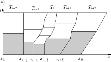
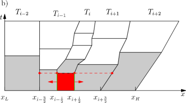
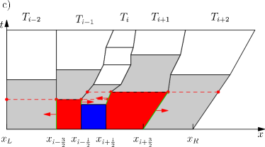
The workflow of an LTS algorithm is best illustrated on a simple example, as the one sketched in Figure 2. For other examples, see [20, 53, 40]. Note that in an LTS algorithm the order in which the elements are updated depends on the update criterion (44). For that reason, one cannot speak of timesteps any more, but the time marching of the LTS code is organized by cycles. In each cycle, the scheme runs over all elements of the domain and skips those which do not satisfy the update criterion (44). This verification is very fast and does not add much computational overhead to the scheme. For the example used here, we suppose $M=1$, hence a second order scheme in space and time is used, for which the criteria (5) and (44) are the same. In this example, suppose that elements $T_{i-2}$ and $T_{i+2}$ are on the boundary of the domain, hence they have to fulfill the update criterion only with respect to neighbors within the computational domain.

Figure 2: Sketch of the ALE-LTS procedure and the generated space-time mesh. Red space-time cells are currently being updated, blue space-time cells have already been updated at least once and space-time cells with an available predictor solution $\mathbf{q}_{h}$ are highlighted in grey. The flux time intervals are depicted in green, the red arrows denote saving of flux contributions in memory variables of neighbor cells and the horizontal dashed red lines indicate reconstruction using virtual data obtained by interpolation from the space-time predictor $\mathbf{q}_{h}$. Note the hanging nodes in time produced by the ALE-LTS algorithm on the element edges.

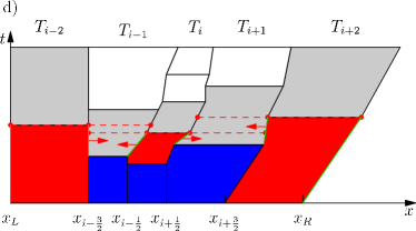At the beginning of the time marching, all elements are defined at the common initial time $t=0$. The cell averages are defined by the initial condition and the first WENO reconstruction can be done for all elements directly based on the cell averages $\mathbf{Q}_{j}$, without the use of the virtual geometry or the virtual cell averages $\tilde{\mathbf{Q}}_{j}$. For each element an element-local time step is defined according to the local CFL condition (48). Note that for the computation of the first time step, the real geometry and the real cell averages can be used in (48) instead of the virtual ones. After reconstruction and local time step computation, each element can compute its element-local predictor solution $\mathbf{q}_{h}$. We are now in the situation depicted in Figure 2 a). All cells are at the same initial time $t=0$, have different time steps and have computed their predictor $\mathbf{q}_{h}(x,t)$, which is valid through one local time step. The intervals with a valid space-time predictor solution $\mathbf{q}_{h}(x,t)$ are highlighted in grey in Figure 2. In the first cycle, only element $T_{i}$ satisfies the update criterion (44), hence it is updated according to the finite volume scheme (6), since on both element interfaces $x_{i\pm\frac{1}{2}}$ the necessary data for flux calculation is available under the form of the predictor $\mathbf{q}_{h}$. The updated cell is highlighted in red in Figure 2 b) and the corresponding flux intervals in time according to Eqn. (7) are highlighted in green. Note that the geometry is updated only for the nodes attached to the element which is updated, hence $x_{i-\frac{1}{2}}$ and $x_{i+\frac{1}{2}}$ advance in time, while the other nodes are still at their old time level. Once the fluxes for cell $T_{i}$ have been computed, they are added to the memory variables $\mathbf{Q}_{i\pm 1}^{M}$ of the neighbor cells (red arrows in Figure 2) and the memory variable $\mathbf{Q}_{i}^{M}$ is reset to zero, according to (10). Now, the local time of cell $T_{i}$ is advanced by a local time step and reconstruction is performed for cell $T_{i}$ at the new local time $t_{i}^{n}$. Since reconstruction requires information from the neighbor cells $T_{i\pm 1}$, which are still at the initial time $t=0$, the reconstruction operator uses the virtual data defined in (42) and a virtual geometry according to (43), which are both computed from the local space-time predictor $\mathbf{q}_{h}(x,t)$. This reconstruction based on virtual data is highlighted by the dashed red horizontal lines in Figure 2. After reconstruction, cell $T_{i}$ can compute its predictor, highlighted again in grey in Figure 2 b), and the first cycle is complete, since no other cells satisfy the update criterion. The second cycle is depicted in Figure 2 c). Now, cells $T_{i-1}$ and $T_{i+1}$ satisfy the update criterion and thus they are both updated in the same cycle. The resulting flux time intervals according to Eqn. (7) are highlighted again in green. One can note in Figure 2 c) that the part of the fluxes which has already been computed previously by element $T_{i}$ and has been saved into the memory variables of $T_{i+1}$ and $T_{i-1}$ is not computed again, but only the missing parts of the time intervals that are necessary to reach the future times $t_{i+1}^{n+1}$ and $t_{i-1}^{n+1}$, respectively. Again, the computed fluxes are added to the memory variables of the neighbor elements, hence $T_{i-1}$ adds the corresponding flux contributions to element $T_{i-2}$ on the left and to $T_{i}$ on the right, see the red arrows in Figure 2 c). Likewise, element $T_{i+1}$ contributes to the memory variables of $T_{i}$ and $T_{i+2}$. After resetting their memory variables, elements $T_{i-1}$ and $T_{i+1}$ perform the reconstruction using the virtual geometry and data provided by the space-time predictor $\mathbf{q}_{h}$ in the neighbor elements, see the dashed lines in Figure 2. After reconstruction, the predictor is computed again, see the grey shaded areas of elements $T_{i-1}$ and $T_{i+1}$. Since in the same cycle no other elements fulfill the update criterion, the cycle ends and we have the situation depicted in Figure 2 d). The three elements that have been updated so far are highlighted in blue, and the elements that satisfy the update criterion within this cycle are $T_{i-2}$, $T_{i}$ and $T_{i+2}$. As in the previous cycles, the flux time intervals are highlighted in green, the communication with the memory variables of the neighbor elements is indicated by the red arrows and the reconstruction based on the virtual data is highlighted by the red dashed horizontal lines. Recall also, that the space-time mesh depicted in Figure 2 is constructed dynamically in each cycle according to the local CFL condition (48) and the Lagrangian mesh motion. It is further important to note that only the spatial nodes attached to the elements that are updated (highlighted in red) are advanced in time. The other nodes remain at their old position at their old time. The resulting space-time mesh is non-conforming in time. As a direct consequence, hanging nodes in time appear, which are conveniently treated by the algorithm using memory variables and the fact that the flux time integrals are additive. The concept of memory variables has first been introduced for LTS methods in [20].

3 Numerical Test problems

In this section, the numerical approach presented above is validated on a large set of one-dimensional Riemann problems for the Euler equations of compressible gas dynamics and the equations of ideal magnetohydrodynamics (MHD). Furthermore, a detailed numerical convergence study is presented for the MHD system for a smooth, non-trivial time-dependent test case.

3.1 Euler equations of compressible gas dynamics

For the first set of shock tube problems the classical Euler equations of compressible gasdynamics are considered. In one space dimension they read

$$\frac{\partial}{\partial t}\left(\begin{array}[]{c}\rho\\ \rho u\\ \rho E\end{array}\right)+\frac{\partial}{\partial x}\left(\begin{array}[]{c}\rho u\\ \rho u^{2}+p\\ u(\rho E+p)\\ \end{array}\right)=0,$$ (49)

with

$$p=(\gamma-1)(\rho E-\frac{1}{2}\rho u^{2}),$$ (50)

where $\rho$ is the mass density, $u$ is the velocity, $p$ is the gas pressure, $\rho E$ is the total energy density and $\gamma$ is the ratio of specific heats.

The initial conditions for the four Riemann problems RP1 - RP4 solved in the following are all of the type,

$$\mathbf{Q}(x,0)=\left\{\begin{array}[]{ccc}\mathbf{Q}_{L}&\textnormal{ if }&x\leq x_{d},\\ \mathbf{Q}_{R}&\textnormal{ if }&x>x_{d}.\end{array}\right.$$ (51)

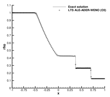
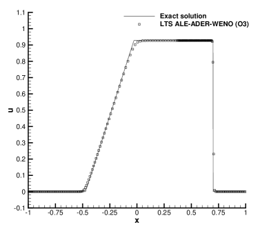
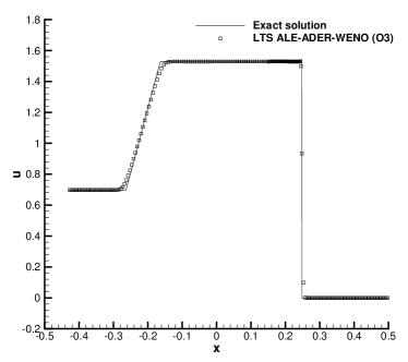
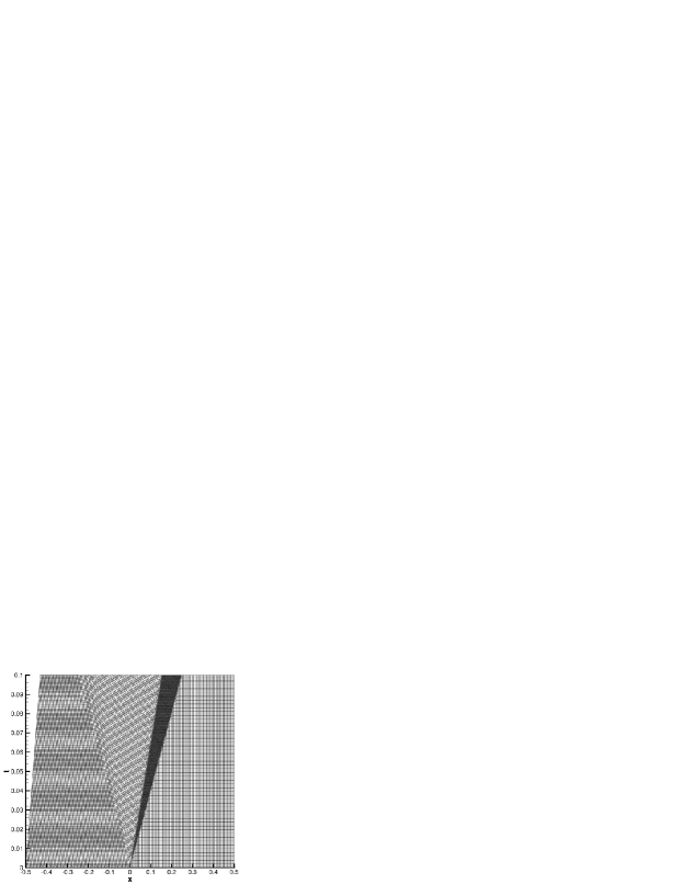
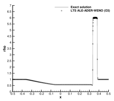
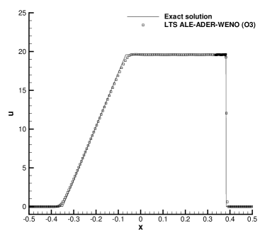
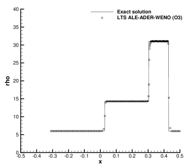
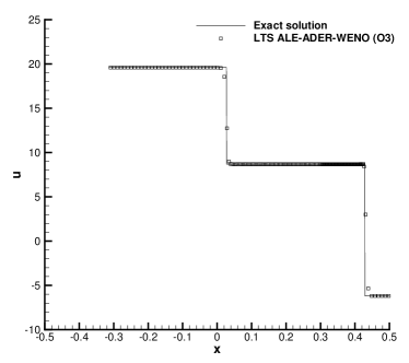
The initial left and right states are listed in detail in Table 1, together with the initial position of the discontinuity $x_{d}$ and the final simulation time $t_{\textnormal{end}}$. The initial computational domain is $\Omega(0)=[x_{L};x_{R}]$, where $x_{L}$ and $x_{R}$ can be easily identified for each problem from the bottom of Figures 3-6; in all cases $\gamma=1.4$. RP1 and RP2 are the classical Sod and Lax shock tube problems, respectively, while RP3 and RP4 are taken from [56]. The exact solution has been computed using the exact Riemann solver described in great detail in [56], where also a full FORTRAN listing is available.

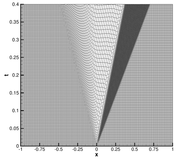
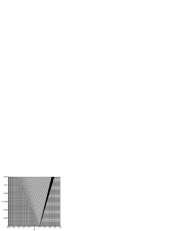
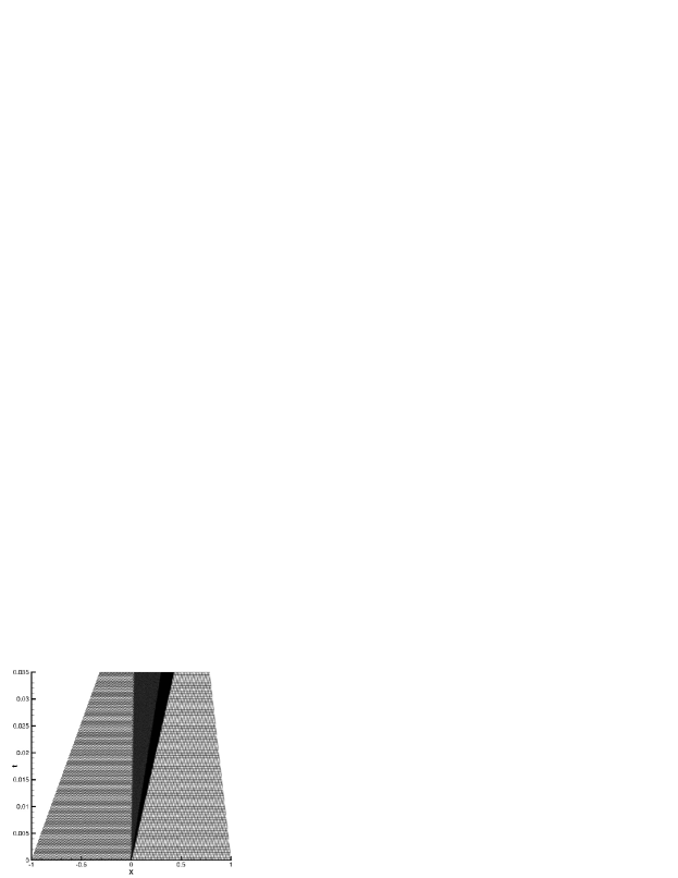
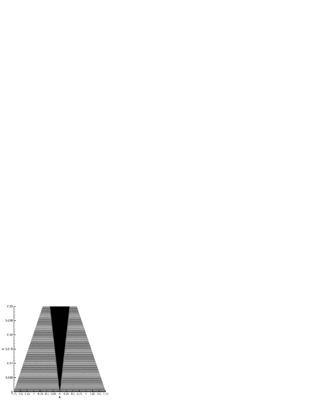
The computational results obtained for density $\rho$ and velocity $u$ with a third order ADER-WENO scheme (degree of the reconstruction polynomial $M=2$) are depicted together with the exact solution in the top row of Figures 3-6. The Osher-type flux (14) is used in all cases. The initial spatial mesh consists of 200 initially equidistant control volumes for all test problems and the local CFL number is chosen as CFL=0.5. From the computational results one can observe that the contact wave is very well resolved and that the results are essentially non-oscillatory. Note that the scheme presented in this article is not purely Lagrangian, but it is of the direct ALE type, hence a non-vanishing mass flux through the contact wave is possible, which leads to a small, but visible, smearing of the contact discontinuity (see Figures 3-6). The resulting space-time mesh for all test cases is shown in the bottom row of Figures 3-6. One can clearly identify the emerging wave structure of the Riemann problem, as well as the local time steps, which are given by the vertical extent of each single space-time control volume. Furthermore, the space-time meshes also show the hanging nodes in time that arise within the LTS algorithm. For all cases RP1-RP4 it has been explicitly verified that the relative conservation error was of the order of machine accuracy for all conserved quantities. The total absolute conservation error at the final simulation time is listed for each test problem and for all conserved quantities in Table 2, together with the necessary total number of element updates when using a local time-stepping algorithm (LTS) or a traditional method based on global time stepping (GTS). The last column of Table 2 contains the savings factor, which clearly indicates that for the test problems considered here, a substantial savings in element updates can be achieved by using an LTS strategy.

Table 1: Initial states left and right for the density $\rho$, velocity $u$ and the pressure $p$ for the compressible Euler equations. The final output times, ($t_{\textnormal{end}}$) and the initial position of the discontinuity ($x_{d}$) are also given.

Case	$\rho_{L}$	$u_{L}$	$p_{L}$	$\rho_{R}$	$u_{R}$	$p_{R}$	$t_{\textnormal{end}}$	$x_{d}$
RP1	1.0	0.0	1.0	0.125	0.0	0.1	0.4	0.0
RP2	0.445	0.698	3.528	0.5	0.0	0.571	0.1	0.0
RP3	1.0	0.0	1000	1.0	0.0	0.01	0.012	0.1
RP4	5.99924	19.5975	460.894	5.99242	-6.19633	46.095	0.035	-0.2

Figure 3: Exact and numerical solution for the Sod shock tube problem. Density (top left), velocity (top right) and resulting space-time mesh of the third order Lagrangian ADER-WENO finite volume scheme with conservative and time-accurate local time stepping (bottom).

Figure 4: Exact and numerical solution for the Lax shock tube problem. Density (top left), velocity (top right) and resulting space-time mesh of the third order Lagrangian ADER-WENO finite volume scheme with conservative and time-accurate local time stepping (bottom).

Figure 5: Exact and numerical solution for shock tube problem RP3. Density (top left), velocity (top right) and resulting space-time mesh of the third order Lagrangian ADER-WENO finite volume scheme with conservative and time-accurate local time stepping (bottom).

Figure 6: Exact and numerical solution for shock tube problem RP4. Density (top left), velocity (top right) and resulting space-time mesh of the third order Lagrangian ADER-WENO finite volume scheme with conservative and time-accurate local time stepping (bottom).

Table 2: Euler equations: Total absolute conservation error for each test case and comparison of the computational efficiency between GTS and LTS algorithm using the total number of element updates.

	Conservation error			Number of element updates
Case	$\rho$	$\rho u$	$\rho E$	GTS	LTS	GTS/LTS
RP1	2.08944E-13	4.60021E-13	9.86766E-13	73600	21840	3.37
RP2	2.24598E-13	1.69381E-12	7.67386E-12	65000	20579	3.16
RP3	1.13805E-11	9.82959E-10	5.47216E-08	167000	34222	4.88
RP4	1.23741E-11	3.40464E-10	5.94946E-09	294800	50481	5.84

3.2 Ideal classical MHD equations

In this section the equations of ideal classical magnetohydrodynamics (MHD) are solved with the proposed Arbitrary-Lagrangian-Eulerian ADER-WENO finite volume scheme, together with the new local time stepping (LTS) feature. The augmented PDE system including the hyperbolic divergence-correction term proposed by Dedner et al. [13] reads

$$\frac{\partial}{\partial t}\left(\begin{array}[]{c}\rho\\ \rho\vec{v}\\ \rho E\\ \vec{B}\\ \psi\end{array}\right)+\nabla\cdot\left(\begin{array}[]{c}\rho\vec{v}\\ \rho\vec{v}\vec{v}+p_{t}\mathbf{I}-\frac{1}{4\pi}\vec{B}\vec{B}\\ \vec{v}(\rho E+p_{t})-\frac{1}{4\pi}\vec{B}(\vec{v}\cdot\vec{B})\\ \vec{v}\vec{B}-\vec{B}\vec{v}+\psi\mathbf{I}\\ c_{h}^{2}\vec{B}\end{array}\right)=0,$$ (52)

with

$$p=(\gamma-1)(\rho E-\frac{1}{2}\rho\vec{v}^{2}-\frac{1}{8\pi}\vec{B}^{2}),\qquad p_{t}=p+\frac{1}{8\pi}\vec{B}^{2}.$$ (53)

In Eqn. 52, $\rho$ is the density of the gas, $\vec{v}=(u,v,w)$ is the velocity vector, $\vec{B}=(B_{x},B_{y},B_{z})$ is the vector of the magnetic field, $p$ is the gas pressure, $p_{t}$ is the sum of the gas and the magnetic pressure, $\rho E$ is the total energy density and $\gamma$ is the ratio of specific heats. $\mathbf{I}$ is the unit matrix and the notation $\vec{x}_{1}\vec{x}_{2}$ denotes the dyadic product of two vectors $\vec{x}_{1}$ and $\vec{x}_{2}$. The scalar $\psi$ is used for divergence cleaning, see [13], to satisfy the constraint $\nabla\cdot\vec{B}=0$. In one space dimension, this constraint simply reduces to $\partial B_{x}/\partial x=0$.

In the following one-dimensional test problems either the classical Rusanov flux (13) is used, or the new Osher-type flux given by Eqn. (14), which has been originally proposed by Dumbser and Toro for the Eulerian case in [21, 22] and has subsequently been extended to Lagrangian schemes in [23].

Riemann problems

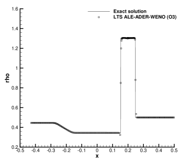
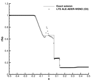
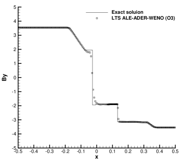
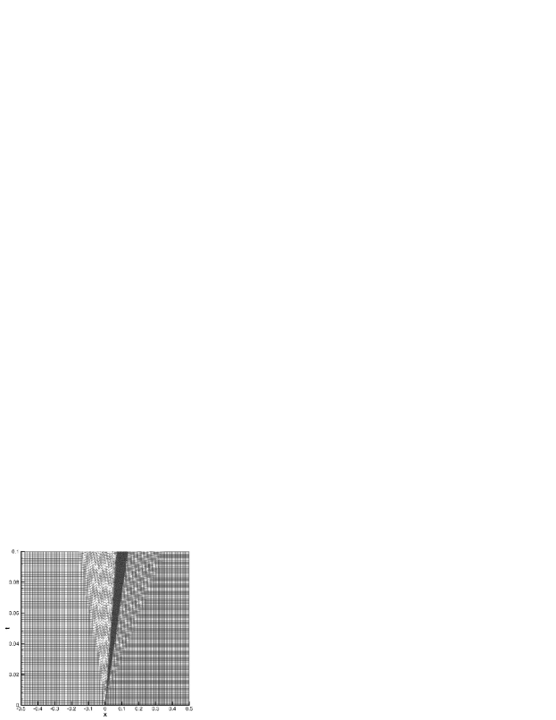
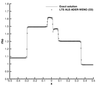
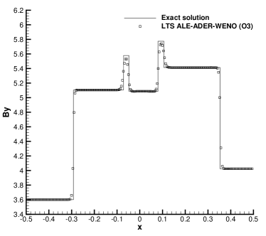
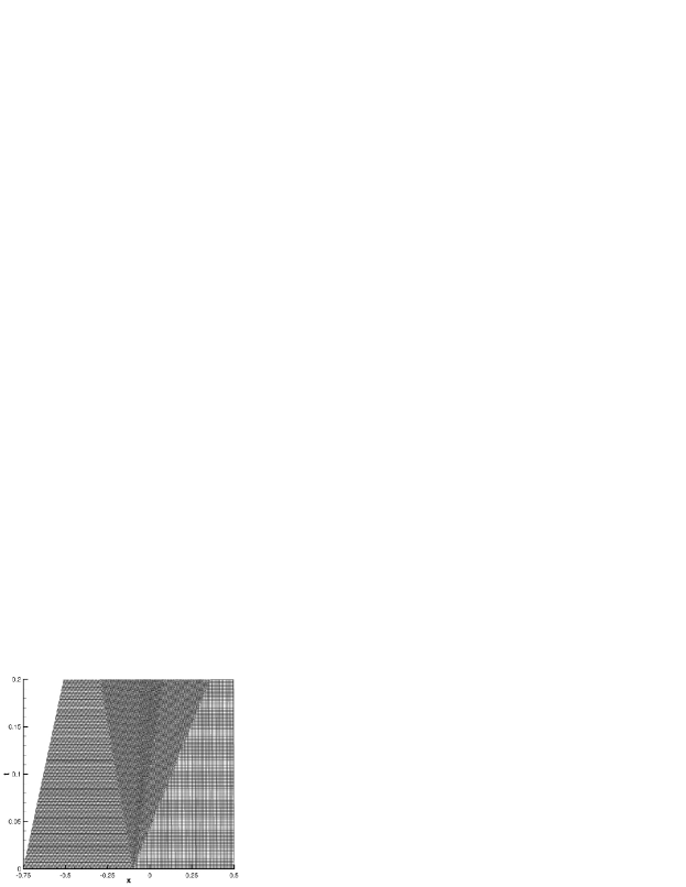
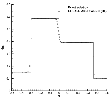
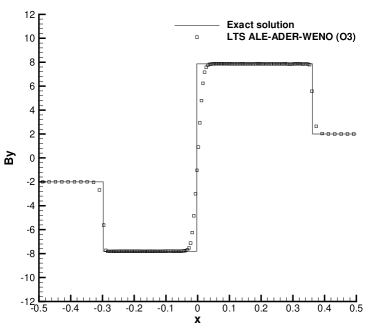
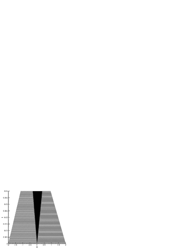
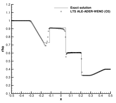
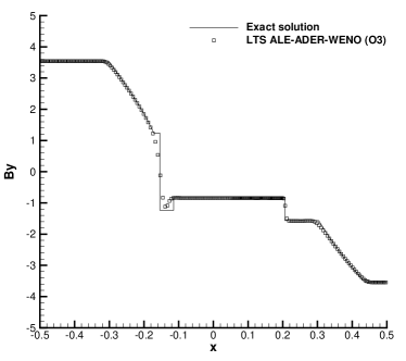
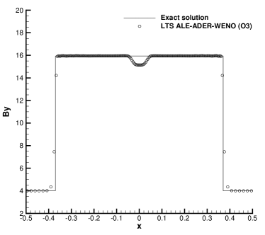
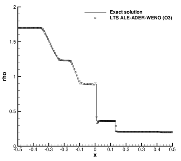
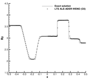
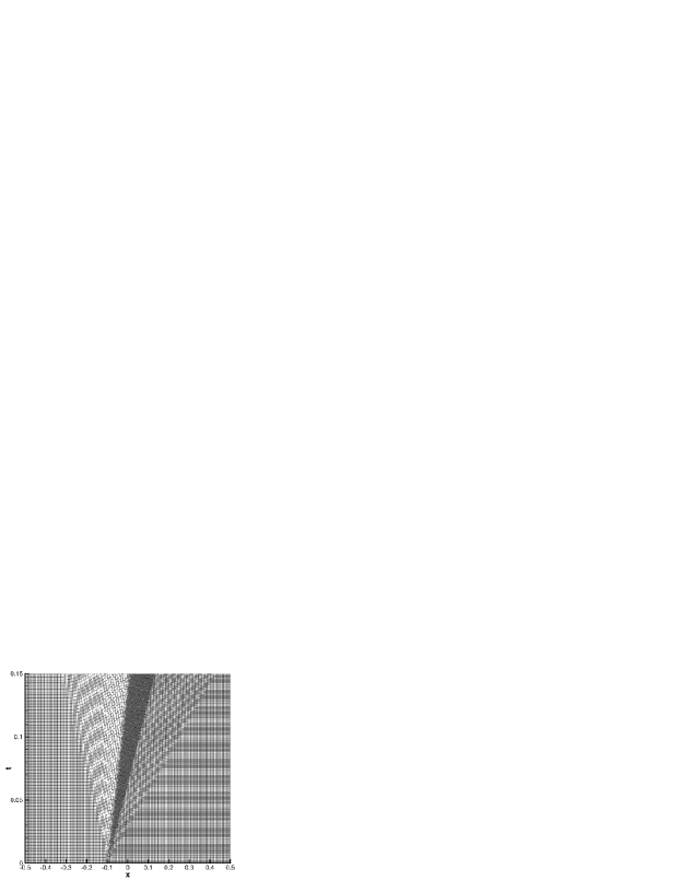
The initial conditions for the shock tube problems are listed in Table 3 and the ratio of specific heats is set to $\gamma=\frac{5}{3}$ for all cases. All shock-tube problems are solved on a mesh of 200 initially equidistant cells using the third order version of the ALE ADER-WENO scheme with LTS. The computational results are depicted in Figs. 7 to 12, together with the exact solution and the resulting space-time meshes. The exact Riemann solver for MHD has kindly been provided by S.A.E.G. Falle [27]. For an alternative exact Riemann solver of the MHD equations, see also [57]. In all cases, the numerical results agree well with the exact solution, the contact wave is well resolved and most of the details of the wave structure emerging from the Riemann problem are properly resolved. As can be seen from Figures 7-12 the space-time mesh directly reflects the wave pattern of the Riemann problem, as expected. One can furthermore observe that in those regions where the mesh is compressed by the presence of a shock wave, the time step is locally decreased, while inside the rarefaction fans, where the mesh is expanding, the time step is locally increased. To assess the efficiency of the proposed local time stepping algorithm, the total number of element updates is reported for all test problems in Table 4. Furthermore, the total conservation error at the final time is reported for each test case in Table 4, showing that also with the use of an LTS strategy a conservative scheme can be designed in the framework of high order Lagrangian finite volume schemes.

Table 3: Initial states left and right for the density $\rho$, velocity vector $\vec{v}=(u,v,w)$, the pressure $p$ and the magnetic field vector $\vec{B}=(B_{x},B_{y},B_{z})$ for the ideal classical MHD equations. The final output times, ($t_{\textnormal{end}}$) and the initial position of the discontinuity ($x_{d}$) are also given. In all cases $\gamma=5/3$.

Case	$\rho$	$u$	$v$	$w$	$p$	$B_{x}$	$B_{y}$	$B_{z}$	$t_{\textnormal{end}}$, $x_{d}$
RP1 L:	1.0	0.0	0.0	0.0	1.0	$\frac{3}{4}\sqrt{4\pi}$	$\sqrt{4\pi}$	0.0	0.1
R:	0.125	0.0	0.0	0.0	0.1	$\frac{3}{4}\sqrt{4\pi}$	$-\sqrt{4\pi}$	0.0	0.0
RP2 L:	1.08	1.2	0.01	0.5	0.95	2.0	3.6	2.0	0.2
R:	0.9891	-0.0131	0.0269	0.010037	0.97159	2.0	4.0244	2.0026	-0.1
RP3 L:	0.15	21.55	1.0	1.0	0.28	0.05	-2.0	-1.0	0.04
R:	0.1	-26.45	0.0	0.0	0.1	0.05	2.0	1.0	0.0
RP4 L:	1.0	0.0	0.0	0.0	1.0	$1.3\sqrt{4\pi}$	$\sqrt{4\pi}$	0.0	0.16
R:	0.4	0.0	0.0	0.0	0.4	$1.3\sqrt{4\pi}$	$-\sqrt{4\pi}$	0.0	0.0
RP5 L:	1.0	36.87	-0.115	-0.0386	1.0	4.0	4.0	1.0	0.03
R:	1.0	-36.87	0.0	0.0	1.0	4.0	4.0	1.0	0.0
RP6 L:	1.7	0.0	0.0	0.0	1.7	3.899398	3.544908	0.0	0.15
R:	0.2	0.0	0.0	-1.496891	0.2	3.899398	2.785898	2.192064	-0.1

Figure 7: Exact and numerical solution for the MHD shock tube problem RP1. Density (top left), magnetic field component $B_{y}$ (top right) and resulting space-time mesh of the third order Lagrangian ADER-WENO finite volume scheme with conservative and time-accurate local time stepping (bottom).

Figure 8: Exact and numerical solution for the MHD shock tube problem RP2. Density (top left), magnetic field component $B_{y}$ (top right) and resulting space-time mesh of the third order Lagrangian ADER-WENO finite volume scheme with conservative and time-accurate local time stepping (bottom).

Figure 9: Exact and numerical solution for the MHD shock tube problem RP3. Density (top left), magnetic field component $B_{y}$ (top right) and resulting space-time mesh of the third order Lagrangian ADER-WENO finite volume scheme with conservative and time-accurate local time stepping (bottom).

Figure 10: Exact and numerical solution for the MHD shock tube problem RP4. Density (top left), magnetic field component $B_{y}$ (top right) and resulting space-time mesh of the third order Lagrangian ADER-WENO finite volume scheme with conservative and time-accurate local time stepping (bottom).

Figure 11: Exact and numerical solution for the MHD shock tube problem RP5. Density (top left), magnetic field component $B_{y}$ (top right) and resulting space-time mesh of the third order Lagrangian ADER-WENO finite volume scheme with conservative and time-accurate local time stepping (bottom).

Figure 12: Exact and numerical solution for the MHD shock tube problem RP6. Density (top left), magnetic field component $B_{y}$ (top right) and resulting space-time mesh of the third order Lagrangian ADER-WENO finite volume scheme with conservative and time-accurate local time stepping (bottom).

Table 4: MHD equations: Conservation error for each test case and comparison of the computational efficiency between GTS and LTS algorithm using the total number of element updates.

	Conservation error					Number of element updates
Case	$\rho$	$\rho u$	$\rho v$	$\rho E$	$B_{y}$	GTS	LTS	GTS/LTS
RP1	1.188E-13	5.066E-13	5.117E-13	2.608E-12	8.825E-12	23060	49400	2.14
RP2	7.159E-13	1.006E-12	1.489E-12	6.823E-12	8.284E-12	36313	50600	1.39
RP3	1.616E-12	3.407E-11	1.618E-12	3.888E-10	2.117E-11	33635	69000	2.05
RP4	5.282E-13	2.857E-12	2.356E-12	5.349E-12	1.559E-11	29727	40200	1.35
RP5	2.770E-12	9.040E-11	3.176E-12	1.714E-09	1.136E-11	48383	93600	1.93
RP6	2.139E-13	7.934E-13	3.722E-13	8.717E-13	2.140E-12	36234	70800	1.95

Convergence study

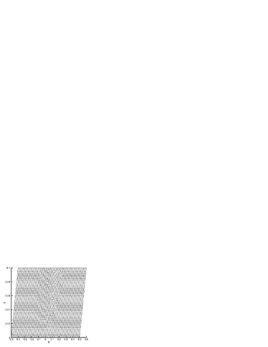
Here we solve a smooth time-dependent problem for the MHD equations with exact solution, so that the designed order of accuracy in space and time of the proposed Lagrangian ADER-WENO scheme with LTS can be verified. The problem consists in a traveling Alfvén wave and the exact solution of the problem is given by $\rho(x,t)=1$, $u(x,t)=0$, $v(x,t)=1-A\exp(-\frac{1}{2}(x-v_{a}t)^{2}/\sigma^{2})$, $w(x,t)=-\sqrt{2-v(x,t)^{2}}$, $p(x,t)=1$, $B_{x}(x,t)=\sqrt{4\pi}$, $B_{y}(x,t)=-\sqrt{4\pi}v(x,t)$ and $B_{z}(x,t)=\sqrt{4\pi}\sqrt{2-v(x,t)^{2}}$, with the Alfvén speed $v_{a}=1$. The amplitude and the halfwidth of the perturbation are given by $A=0.1$ and $\sigma=0.25$, respectively. The simulation is run with third to fifth order schemes based on the Osher-type flux (14). The initial domain is $\Omega(0)=[-2;2]$. In this simulation the mesh velocity has been chosen as $V=v$ to get a non-trivial mesh motion. The convergence rates for variable $B_{y}$ at a final time of $t=0.1$ are reported in Table 5, where the number of grid cells used to discretize the domain $\Omega(t)$ is denoted by $N_{G}$. From the obtained results one can conclude that the designed high order of accuracy in space and time of the Lagrangian ADER-WENO schemes is maintained when the local time stepping feature (LTS) presented in this article is used. An example of a resulting space-time mesh is depicted for the grid $N_{G}=100$ in Figure 13.

Table 5: Numerical convergence results for the ideal MHD equations using third to fifth order Lagrangian ADER-WENO finite volume schemes with time accurate local time stepping (LTS). The error norms refer to the variable $B_{y}$ (density) at time $t=0.1$.

$N_{G}$	$\epsilon_{L_{2}}$	$\mathcal{O}(L_{2})$	$N_{G}$	$\epsilon_{L_{2}}$	$\mathcal{O}(L_{2})$	$N_{G}$	$\epsilon_{L_{2}}$	$\mathcal{O}(L_{2})$
$\mathcal{O}3$			$\mathcal{O}4$			$\mathcal{O}5$
100	2.1272E-04		25	3.1389E-03		25	1.5085E-03
200	9.3217E-06	4.51	100	4.9217E-06	4.66	100	2.6843E-06	4.57
400	1.1615E-06	3.00	200	2.0642E-07	4.58	150	3.6715E-07	4.91
800	1.4502E-07	3.00	300	3.2271E-08	4.58	200	8.9272E-08	4.92

Figure 13: Space-time mesh for the numerical convergence study using a grid with 100 mesh points.

4 Conclusions

To the knowledge of the author, this is the first time that a high order Lagrangian finite volume scheme with time-accurate local time stepping (LTS) has been presented. The design principle of the method is the use of a non-conforming space-time mesh. High order of accuracy in time is achieved via a local space-time discontinuous Galerkin predictor, which solves element-local Cauchy problems using a weak form of the PDE in space-time. The initial condition of these local Cauchy problems is given by a high order WENO reconstruction. Since the cell averages and the spatial grid points are usually defined at different time levels, the reconstruction operator is applied on a virtual geometry and a virtual set of cell averages that can be easily computed via $L_{2}$ projection using the space-time predictor. The fluxes are computed in a consistent and conservative way using memory variables, which allow to handle the non-conforming nodes in time very easily from an algorithmic point of view.

The algorithm has been applied to the Euler equations of compressible gas dynamics and to the ideal MHD equations. A set of 1D Riemann problems has been solved for both systems of conservation laws. Furthermore, numerical convergence results on a smooth unsteady test problem with exact solution have been shown for the MHD system using third to fifth order schemes in space and time.

Future research will concern the extension of the local time-stepping algorithm presented in this paper to the multi-dimensional ALE ADER-WENO schemes presented in [5, 6, 16].

References

- [1] A. Baeza, A. Martínez-Gavara, and P. Mulet. Adaptation based on interpolation errors for high order mesh refinement methods applied to conservation laws . Applied Numerical Mathematics, 62:278–296, 2012.
- [2] A. Baeza and P. Mulet. Adaptive mesh refinement techniques for high-order shock capturing schemes for multi-dimensional hydrodynamic simulations. International Journal for Numerical Methods in Fluids, 52:455–471, 2006.
- [3] M. Berndt, J. Breil, S. Galera, M. Kucharik, P.H. Maire, and M.J. Shashkov. Two-step hybrid conservative remapping for multimaterial arbitrary Lagrangian-Eulerian methods. Journal of Computational Physics, 230:6664–6687, 2011.
- [4] P. Bochev, D. Ridzal, and M.J. Shashkov. Fast optimization-based conservative remap of scalar fields through aggregate mass transfer. Journal of Computational Physics, 246:37–57, 2013.
- [5] W. Boscheri and M. Dumbser. Lagrangian ADER–WENO Finite Volume Schemes on Unstructured Tetrahedral Meshes for Conservative and Nonconservative Hyperbolic Systems in 3D. Journal of Computational Physics. submitted to.
- [6] W. Boscheri and M. Dumbser. Arbitrary–Lagrangian–Eulerian One–Step WENO Finite Volume Schemes on Unstructured Triangular Meshes. Communications in Computational Physics, 14:1174–1206, 2013.
- [7] R. Bürger, P. Mulet, and L.M. Villada. Spectral weno schemes with adaptive mesh refinement for models of polydisperse sedimentation. ZAMM - Journal of Applied Mathematics and Mechanics / Zeitschrift für angewandte Mathematik und Mechanik, pages n/a–n/a, 2012.
- [8] G. Carré, S. Del Pino, B. Després, and E. Labourasse. A cell-centered lagrangian hydrodynamics scheme on general unstructured meshes in arbitrary dimension. Journal of Computational Physics, 228:5160–5183, 2009.
- [9] C.E. Castro, M. Käser, and E.F. Toro. Space–time adaptive numerical methods for geophysical applications. Philosophical Transactions of the Royal Society A: Mathematical, Physical and Engineering Sciences, 367:4613–4631, 2009.
- [10] J. Cheng and C.W. Shu. A high order ENO conservative Lagrangian type scheme for the compressible Euler equations. Journal of Computational Physics, 227:1567–1596, 2007.
- [11] J. Cheng and C.W. Shu. A cell-centered Lagrangian scheme with the preservation of symmetry and conservation properties for compressible fluid flows in two-dimensional cylindrical geometry. Journal of Computational Physics, 229:7191–7206, 2010.
- [12] J. Cheng and E.F. Toro. A 1D conservative Lagrangian ADER scheme. Chinese Journal of Computational Physics, 30:501–508, 2013.
- [13] A. Dedner, F. Kemm, D. Kröner, C.-D. Munz, T. Schnitzer, and M. Wesenberg. Hyperbolic divergence cleaning for the MHD equations. Journal of Computational Physics, 175:645–673, 2002.
- [14] B. Després and C. Mazeran. Lagrangian gas dynamics in two-dimensions and lagrangian systems. Archive for Rational Mechanics and Analysis, 178:327–372, 2005.
- [15] M. Dumbser. Arbitrary high order PNPM schemes on unstructured meshes for the compressible Navier–Stokes equations. Computers & Fluids, 39:60–76, 2010.
- [16] M. Dumbser and W. Boscheri. High–Order Unstructured Lagrangian One–Step WENO Finite Volume Schemes for Non–conservative Hyperbolic Systems: Applications to Compressible Multi–Phase Flows. Computers and Fluids, 86:405–432, 2013.
- [17] M. Dumbser, C. Enaux, and E.F. Toro. Finite volume schemes of very high order of accuracy for stiff hyperbolic balance laws. Journal of Computational Physics, 227:3971–4001, 2008.
- [18] M. Dumbser and M. Käser. Arbitrary high order non-oscillatory finite volume schemes on unstructured meshes for linear hyperbolic systems. Journal of Computational Physics, 221:693–723, 2007.
- [19] M. Dumbser, M. Käser, V.A Titarev, and E.F. Toro. Quadrature-free non-oscillatory finite volume schemes on unstructured meshes for nonlinear hyperbolic systems. Journal of Computational Physics, 226:204–243, 2007.
- [20] M. Dumbser, M. Käser, and E. F. Toro. An arbitrary high order discontinuous Galerkin method for elastic waves on unstructured meshes V: Local time stepping and -adaptivity. Geophysical Journal International, 171:695–717, 2007.
- [21] M. Dumbser and E. F. Toro. On universal Osher–type schemes for general nonlinear hyperbolic conservation laws. Communications in Computational Physics, 10:635–671, 2011.
- [22] M. Dumbser and E. F. Toro. A simple extension of the Osher Riemann solver to non-conservative hyperbolic systems. Journal of Scientific Computing, 48:70–88, 2011.
- [23] M. Dumbser, A. Uuriintsetseg, and O. Zanotti. On Arbitrary–Lagrangian–Eulerian One–Step WENO Schemes for Stiff Hyperbolic Balance Laws. Communications in Computational Physics, 14:301–327, 2013.
- [24] M. Dumbser and O. Zanotti. Very high order PNPM schemes on unstructured meshes for the resistive relativistic MHD equations. Journal of Computational Physics, 228:6991–7006, 2009.
- [25] M. Dumbser, O. Zanotti, A. Hidalgo, and D.S. Balsara. ADER-WENO Finite Volume Schemes with Space-Time Adaptive Mesh Refinement. Journal of Computational Physics, 248:257–286, 2013.
- [26] M. Dumbser, O. Zanotti, A. Hidalgo, and D.S. Balsara. High Order Space-Time Adaptive ADER–WENO Finite Volume Schemes for Non–Conservative Hyperbolic Systems. Computer Methods in Applied Mechanics and Engineering, 268:359–387, 2014.
- [27] S.A.E.G. Falle. On the inadmissibility of non-evolutionary shocks. Journal of Plasma Physics, 65:29–58, 2001.
- [28] J. Flaherty, R. Loy, M. Shephard, B. Szymanski, J. Teresco, and L. Ziantz. Adaptive local refinement with octree load–balancing for the parallel solution of three–dimensional conservation laws. Journal of Parallel and Distributed Computing, 47:139–152, 1997.
- [29] G. Gassner, F. Lörcher, and C. D. Munz. A discontinuous Galerkin scheme based on a space-time expansion II. viscous flow equations in multi dimensions. Journal of Scientific Computing, 34:260–286, 2008.
- [30] M.J. Grote and T. Mitkova. Explicit local time-stepping methods for Maxwell’s equations. Journal of Computational and Applied Mathematics, 234:3283–3302, 2010.
- [31] M.J. Grote and T. Mitkova. High-order explicit local time-stepping methods for damped wave equations. Journal of Computational and Applied Mathematics, 239:270–289, 2013.
- [32] A. Harten, B. Engquist, S. Osher, and S. Chakravarthy. Uniformly high order essentially non-oscillatory schemes, III. Journal of Computational Physics, 71:231–303, 1987.
- [33] A. Hidalgo and M. Dumbser. ADER schemes for nonlinear systems of stiff advection diffusion reaction equations. Journal of Scientific Computing, 48:173–189, 2011.
- [34] G.S. Jiang and C.W. Shu. Efficient implementation of weighted ENO schemes. Journal of Computational Physics, 126:202–228, 1996.
- [35] L. Krivodonova. An efficient local time–stepping scheme for solution of nonlinear conservation laws. Journal of Computational Physics, 229:8537–8551, 2010.
- [36] M. Kucharik, J. Breil, S. Galera, P.H. Maire, M. Berndt, and M.J. Shashkov. Hybrid remap for multi-material ALE. Computers and Fluids, 46:293–297, 2011.
- [37] M. Kucharik and M.J. Shashkov. One-step hybrid remapping algorithm for multi-material arbitrary Lagrangian-Eulerian methods. Journal of Computational Physics, 231:2851–2864, 2012.
- [38] R. Liska, M.J. Shashkov P. Váchal, and B. Wendroff. Synchronized flux corrected remapping for ALE methods. Computers and Fluids, 46:312–317, 2011.
- [39] W. Liu, J. Cheng, and C.W. Shu. High order conservative Lagrangian schemes with Lax Wendroff type time discretization for the compressible Euler equations. Journal of Computational Physics, 228:8872–8891, 2009.
- [40] F. Lörcher, G. Gassner, and C. D. Munz. A discontinuous Galerkin scheme based on a space-time expansion. I. inviscid compressible flow in one space dimension. Journal of Scientific Computing, 32:175–199, 2007.
- [41] R. Loubère, P.H. Maire, and M. Shashkov. ReALE: A Reconnection Arbitrary–Lagrangian -Eulerian method in cylindrical geometry. Computers and Fluids, 46:59–69, 2011.
- [42] R. Loubère, P.H. Maire, and P. Váchal. A second–order compatible staggered Lagrangian hydrodynamics scheme using a cell–centered multidimensional approximate Riemann solver. Procedia Computer Science, 1:1931–1939, 2010.
- [43] P.-H. Maire. A high-order one-step sub-cell force-based discretization for cell-centered lagrangian hydrodynamics on polygonal grids. Computers and Fluids, 46(1):341–347, 2011.
- [44] P.-H. Maire. A unified sub-cell force-based discretization for cell-centered lagrangian hydrodynamics on polygonal grids. International Journal for Numerical Methods in Fluids, 65:1281–1294, 2011.
- [45] P.H. Maire. A high-order cell–centered Lagrangian scheme for compressible fluid flows in two–dimensional cylindrical geometry . Journal of Computational Physics, 228:6882–6915, 2009.
- [46] P.H. Maire, R. Abgrall, J. Breil, and J. Ovadia. A cell-centered lagrangian scheme for two-dimensional compressible flow problems. SIAM Journal on Scientific Computing, 29:1781–1824, 2007.
- [47] C.D. Munz. On Godunov–type schemes for Lagrangian gas dynamics. SIAM Journal on Numerical Analysis, 31:17–42, 1994.
- [48] A. López Ortega and G. Scovazzi. A geometrically–conservative, synchronized, flux–corrected remap for arbitrary Lagrangian–Eulerian computations with nodal finite elements. Journal of Computational Physics, 230:6709–6741, 2011.
- [49] V. V. Rusanov. Calculation of Interaction of Non–Steady Shock Waves with Obstacles. J. Comput. Math. Phys. USSR, 1:267–279, 1961.
- [50] S.K. Sambasivan, M.J. Shashkov, and D.E. Burton. A finite volume cell-centered Lagrangian hydrodynamics approach for solids in general unstructured grids. International Journal for Numerical Methods in Fluids, 72:770–810, 2013.
- [51] G. Scovazzi. Lagrangian shock hydrodynamics on tetrahedral meshes: A stable and accurate variational multiscale approach. Journal of Computational Physics, 231:8029–8069, 2012.
- [52] A.H. Stroud. Approximate Calculation of Multiple Integrals. Prentice-Hall Inc., Englewood Cliffs, New Jersey, 1971.
- [53] A. Taube, M. Dumbser, C.D. Munz, and R. Schneider. A High Order Discontinuous Galerkin Method with Local Time Stepping for the Maxwell Equations. International Journal Of Numerical Modelling: Electronic Networks, Devices And Fields, 22:77–103, 2009.
- [54] V.A. Titarev and E.F. Toro. ADER: Arbitrary high order Godunov approach. Journal of Scientific Computing, 17:609–618, 2002.
- [55] V.A. Titarev and E.F. Toro. ADER schemes for three-dimensional nonlinear hyperbolic systems. Journal of Computational Physics, 204:715–736, 2005.
- [56] E.F. Toro. Riemann Solvers and Numerical Methods for Fluid Dynamics. Springer, second edition, 1999.
- [57] M. Torrilhon. Non-uniform convergence of finite volume schemes for Riemann problems of ideal magnetohydrodynamics. Journal of Computational Physics, 192:73–94, 2003.
- [58] J. Utzmann, T. Schwartzkopff, M. Dumbser, and C.D. Munz. Heterogeneous Domain Decomposition for Computational Aeroacoustics. AIAA Journal, 44:2231–2250, 2006.