Melting/freezing transition in polydisperse Lennard-Jones system: Remarkable agreement between predictions of inherent structure, bifurcation phase diagram, Hansen-Verlet rule and Lindemann criteria

Abstract

We use polydispersity in size as a control parameter to explore certain aspects of melting and freezing transitions in a system of Lennard-Jones spheres. Both analytical theory and computer simulations are employed to establish a potentially interesting relationship between observed terminal polydispersity in Lennard-Jones polydisperse spheres and prediction of the same in the integral equation based theoretical analysis of liquid-solid transition. As we increase polydispersity, solid becomes inherently unstable because of the strain built up due to the size disparity. This aspect is studied here by calculating the inherent structure (IS) calculation. With polydispersity at constant volume fraction we find initially a sharp rise of the average IS energy of the crystalline solid until transition polydispersity, followed by a cross over to a weaker dependence of IS energy on polydispersity in the amorphous state. This cross over from FCC to amorphous state predicted by IS analysis agrees remarkably well with the solid-liquid phase diagram (with extension into the metastable phase) generated by non-linear integral equation theories of freezing. Two other well-known criteria of freezing/melting transitions, the Hansen-Verlet rule of freezing and the Lindemann criterion of melting are both shown to be remarkably in good agreement with the above two estimates. Together they seem to indicate a small range of metastability in the liquid-solid transition in polydisperse solids.

I Introduction

In earlier studies of polydisperse system it has been established that homogeneous crystallization never takes place above an upper limit of the polydispersity, known as terminal polydispersity Abraham et al. (2008); Lacks and Wienhoff (1999); Kofke and Bolhuis (1999); Williams et al. (2001); Auer and Frenkel (2001); Hansen and McDonald (2006); Maeda et al. (2003). Recently, an application of density functional theory (DFT) theory of freezing Ramakrishnan and Yussouff (1979); Ramakrishnan (1982) of hard sphere fluid by Chaudhuri et al. found a terminal polydispersity of 0.048, followed by a reentrant melting at larger density  Chaudhuri et al. (2005). Several studies showed the existence of terminal polydispersity as well as reentrant melting Tokuyama and Terada (2005); Bartlett and Warren (1999) on hard sphere polydisperse systems. Experimental studies, however, observed a nearly universal value of 0.12 for the terminal polydispersity Phan et al. (1998); Underwood et al. (1994). A number of theoretical and experimental techniques have been utilized to understand freezing/melting transition Haymet and Oxtoby (1986, 1981); Oxtoby and Haymet (1982); Schneider et al. (1970); Schneider (1971); Yang et al. (1976); Löwen et al. (1993); Löwen and Hoffmann (1999); Singh et al. (1985); Stoessel and Wolynes (1984); Langer (2013); Leocmach et al. (2013); Lovett et al. (1976). Although an analytical study of phase transition of polydisperse system is challenging, there have been a number of studies on fluid-fluid and the fluid-solid transition  Fantoni et al. (2006). Both the freezing and melting transition of polydisperse colloidal system have been examined by Löwen et al Löwen et al. (1993); Löwen and Hoffmann (1999). A series of molecular-dynamics calculations has been carried out to examine melting in the classical Gaussian core model Stillinger and Weber (1980).

In the melting of solids when molecules/atoms interact with each other via a central potential, two empirical criteria have been used extensively to predict transitions. From the melting side one uses the Lindemann criterion Lindemann (1910) which states that at melting temperature, the root mean square displacement exceeds 0.1 of the cell length. The second criterion is the Hansen-Verlet rule of crystallization Hansen and Verlet (1969) that requires the value of the first peak of static structure factor $S(k)$ to exceed 2.85 for freezing. Both these simple criteria are found to hold good for different types of interactions and hence these criteria are considered universal. Lindemann criteria of melting can be investigated using lattice dynamical theory. On the other hand, justification of the Hansen-Verlet rule of crystallization comes from the density functional theory of freezing Ramakrishnan and Yussouff (1979); Ramakrishnan (1982); Haymet and Oxtoby (1986, 1981); Oxtoby and Haymet (1982); Singh et al. (1985). These theories have also been used to understand metastability and nucleation in the liquid-solid phase transition of the polydisperse system.

In the present work we apply both theory and computer simulation to establish a relationship between integral equation theory of freezing and terminal polydispersity during the first order liquid-solid phase transition in polydisperse Lennard-Jones spheres. The inherent structure analysis Wales (2003) further enlightens the understanding of the relationship between transition and stability of the solid.

Integral equation based theoretical analysis of freezing transition has been a subject of great interest for many years. The most successful theory of freezing, the Ramakrishnan-Yussouff theory Ramakrishnan (1982); Ramakrishnan and Yussouff (1979) is also based, at the core, on integral equations that relate the inhomogeneous single particle density to two particle direct correlation function, c(r). This theory employs an expansion of density in a Fourier series where order parameters are the density evaluated at the reciprocal lattice vector components. The resulting equations are solved along with the thermodynamics conditions of equality of chemical potential and equality of pressure.

In fact, relationship between solutions of integral equation theories and liquid-solid transition has been investigated extensively. Many of the previous studies focused on the limiting liquid density beyond which liquid becomes unstable with respect to periodic density waves of the solid. In the analysis of Lovett Lovett (1977), this instability point was identified as $\rho_{l}\vec{C}_{2}\left(\vec{G}\right)=1$. Similar conclusion was reached by Munakata et al Munakata (1977, 1978) in an interesting approach using the correct non-linear integral theories. Rice et al built on these previous analyses, but made the analysis robust by using proper order parameters. In the analysis of Rice et al Bagchi et al. (1983a), $\lambda_{\vec{G}}=1$is identified as the limit of instability or spinodal point, where $\lambda_{\vec{G}}=\rho_{S}\,C(G)$, with $\rho_{S}$as the density of the emerging solid phase.

In addition, enormous theoretical approaches are used to describe the freezing transition directly in terms of the bifurcation of solutions for single density from the homogeneous liquid branch to inhomogeneous branch. This approach also applies essentially the same integral equation that relates the inhomogeneous singlet density to the pair direct correlation function Lovett (1977); Bagchi et al. (1983a); Lovett and Buff (1980); Xu and Rice (2008); Bagchi et al. (1983b); Xu and Rice (2011); Radloff et al. (1984). Interestingly, a terminal point in the bifurcation diagram is achieved where the density of the liquid phase is close to the dense random close packed state of the hard sphere liquid and the density of the solid phase is close to crystal closed packed values Bagchi et al. (1983a). This point can be interpreted as the signature of the end of possible compression in the system.

In the elegant approach of the theory of freezing by Ramakrishnan and Yussouff Ramakrishnan (1982); Ramakrishnan and Yussouff (1979), thermodynamic potential of the system is computed as a function of the order parameters proportionl to the periodic lattice components of the singlet density. This theory employs a nearly exact expression for inhomogeneous density field derived from the density functional theory of statistical mechanics. Free energy is expressed in terms of density fluctuations around the bulk liquid density with n-particle direct correlation functions as the expansion coefficients, as elaborated below.

II Theoretical background

In accordance with the density functional theory of freezing, the density of inhomogeneous solid can be expressed in terms of order parameters $\phi_{0}$ and $\left\{\phi_{\vec{G}}\right\}$ in the following fashion

$$\rho_{s}\left(\vec{R}\right)=\rho_{l}\left(1+\phi_{0}\right)+\rho_{l}\sum_{\vec{G}}\phi_{\vec{G}}\exp\left(i\vec{G}\cdot\vec{R}\right),$$ (1)

where $\rho_{s}\left(\vec{R}\right)$ is the inhomogeneous solid density, $\rho_{l}$ is the liquid density and $\left\{\vec{G}\right\}$ is the set of reciprocal lattice vectors of the chosen lattice. The order parameters $\phi_{0}$ and $\left\{\phi_{\vec{G}}\right\}$ are the expansion coefficients of the inhomogeneous solid density, defined quantitatively below. These quantities can be quantified in the following fashion,

$$\rho_{S}=\frac{1}{\Delta}\int_{\Delta}\rho_{S}\left(\vec{R}\right)d\vec{R},$$ (2)

where integration is over the lattice cell of volume $\Delta.$ Fractional density change $\phi_{0}$ in the transition can clearly be written as $\phi_{0}=\left(\rho_{s}-\rho_{l}\right)/\rho_{l}$. Structural order parameters $\phi_{\vec{G}}$ can be obtained by solving the following integral equations as,

$$\phi_{\vec{G}}=\frac{1}{\Delta}\int\frac{\Delta\rho\left(\vec{R}\right)}{\rho_{l}}e^{-i\vec{G}\cdot\vec{R}}d\vec{R}.$$ (3)

One can introduce a scaling transformation that brings out an interesting generality of the freezing theory as,

$$\lambda_{\vec{G}}=\rho_{s}\vec{C}_{2}\left(\vec{G}\right),$$ (4)

$$\psi_{\vec{G}}=\frac{\rho_{l}}{\rho_{s}}\phi_{\vec{G}}.$$ (5)

where $\vec{C}_{2}\left(\vec{G}\right)=\int dRC(R)e^{i\vec{G}\cdot\vec{R}}.$ Therefore, $\lambda_{\vec{G}}$ and $\psi_{\vec{G}}$ are both dimensionless quantities. $\vec{C}_{2}\left(\vec{G}\right)$ is the Fourier transform of the pair direct correlation function, evaluated at $\vec{G}$. The above transformations lead to the following expression $\psi_{\vec{G}_{n}},$

$$\psi_{\vec{G}_{n}}=\frac{\int_{\Delta}d\vec{R}_{1}\xi_{\vec{G}_{n}}\left(\vec{R}_{1}\right)\exp\left[\sum_{\vec{G}}\psi_{\vec{G}}\lambda_{\vec{G}}\xi_{\vec{G}}\left(\vec{R}_{1}\right)\right]}{\int_{\Delta}d\vec{R}_{1}\exp\left[\sum_{\vec{G}}\psi_{\vec{G}}\lambda_{\vec{G}}\xi_{\vec{G}}\left(\vec{R}_{1}\right)\right]}.$$ (6)

Here $\vec{G}_{n}$ is the n-th reciprocal lattice vector, $\xi_{\vec{G}_{n}}$is the periodic density wave corresponds to the set of $\left\{\vec{G}\right\}$ that has the same magnitude. So,

$$\xi_{G_{\alpha}}(R)=\sum_{\left\{G_{\alpha}\right\}}e^{iG_{\alpha}.\overrightarrow{R}}.$$ (7)

Note that Eq. 6 has a quasi-universal character, as noted by Rice et al Bagchi et al. (1983a). Equation 6 does not require any information about direct correlation function or density of the liquid and the solid phases. Only the lattice type needs to be specified. For the calculation of phase transition parameters, Eq. 6 needs to be supplied by the equality of thermodynamic potential as $\Omega_{s}-\Omega_{l}=0.$

Note that Eq. 6 can also be derived by combining equations of Ramakrishnan-Yussouff and of Haymet-Oxtoby (see Eq. 8 below). The scaling transformation allows one to solve for $\psi_{\vec{G}}$ as a function of $\lambda_{\vec{G}}$without requiring the input of direct correlation function, and the functional form has an interesting character as shown below.

Using the density functional theory, one can obtain the following expression of the grand canonical potential difference between solid and liquid as,

$$\Delta\Omega=\left(\rho_{l}C_{0}-1\right)\phi_{0}+\frac{1}{2}C_{0}\rho_{l}\phi_{0}^{2}+\frac{1}{2}\sum_{\vec{G}}\vec{C}_{2}\left(\vec{G}\right)\phi_{\vec{G}}^{2}$$ (8)

$\Delta\Omega=0$ is the second thermodynamic condition of freezing. Since $\phi_{0}$and $\phi_{\vec{G}}$ are all positive, $\Delta\Omega$ can be zero only if $\left(\rho_{l}C_{0}-1\right)\phi_{0}+\frac{1}{2}C_{0}\rho_{l}\phi_{0}^{2}$ is compensated by $\frac{1}{2}\vec{C}_{2}\left(\vec{G}\right)\phi_{\vec{G}}^{2}$. The above expressions are all for one component liquid. However, as shown by Chaudhuri et al. Chaudhuri et al. (2005), the same expression may be used with an effective $C_{0}$ and effective $\vec{C}_{2}\left(\vec{G}\right)$. The order parameters themselves can be determined by a set of non-linear equations, as shown by Rice et al. Xu and Rice (2008, 2011). Interestingly, in many earlier studies the approach of $\rho_{l}\,\vec{C}_{2}\left(\vec{G}\right)$ to unity was considered as the limit of stability of the liquid towards freezing. A different approach was adopted by Rice et al. Bagchi et al. (1983a). In the present analysis, $\rho_{S}\vec{C}_{2}\left(\vec{G}\right)$ approaches unity.

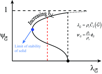
Figure 1: Two order parameter ($\phi_{0}$ and $\phi_{\vec{G}}$) scaled phase diagram plotted in scaled units. The two end points denote two limits of stability. The first terminal point gives the limit of stability of the solid, as discussed here, and is connected to terminal solid density. The second terminal point at $\lambda_{\vec{G}}=1$ gives the limit of stability as discussed earlier by Rice et al. and even earlier by Lovett Lovett (1977).

The scaled phase diagram with scaled variables is shown in Fig. 1. Note this diagram shows a curious character. The scaled phase diagram is just like a van der Waals loop with terminal points that may be identified as the two spinodal points of the solid-liquid phase transition. The first turn is the one that corresponds to the limit of stability of the solid, the second turn at larger density should correspond to the limit of stability of the liquid. Maxwell tie line (given by$\Delta\Omega=0$) is constructed to find coexistence under a given thermodynamic condition. This enforces the additional thermodynamic condition of equality of pressure between the fluid and the solid branches. Eq. 6 and hence the scaled phase diagram have been obtained under the assumption of equality of chemical potential between the liquid and solid phases. Coexistence is found by imposing equality of grand thermodynamic potential (see Eq. 8).

Along X axis, $\lambda_{\vec{G}}$ can correspond to multitudes of $\rho_{S}$ and $\rho_{l}$ values within the region of scaled phase diagram. This is because $\lambda_{\vec{G}}$ depends intricately on both $\rho_{S}$ and $\rho_{l}$ values through direct correlation function which is evaluated with $\rho_{l}$, but at the reciprocal lattice vector $\overrightarrow{G}$ which depends on the solid density $\rho_{S}.$Equality of pressure for grand canonical ensemble picks out unique values of $\rho_{S}$ and $\rho_{l}$. The scaled phase diagram is generated by using same chemical potential, but the condition of equality of pressure needs to be imposed to obtain the thermodynamic transition parameters.

As the polydispersity parameter $\delta$ increases, freezing shifts continuously to higher volume fraction (and pressure). $C_{0}$ increases with density. So, fractional density change decreases to compensate for this as neither $\vec{C}_{2}\left(\vec{G}\right)$ nor $\phi_{\vec{G}}$ undergoes such sharp variation. $\phi_{0}$ decreases as $\rho_{s}$ approaches$\rho_{l}$.

There have been several discussions Bagchi et al. (1983b); Radloff et al. (1984); Bagchi et al. (1984, 1983c) that address the limit of freezing. While Lovett Lovett and Buff (1980) discusses this as a spinodal decomposition, Bagchi-Cerjan-Rice finds this as the last point of the liquid state where the liquid can transform to solid. Beyond this point no solution to integral equation theory is available. Fig. 1 thus provides two densities of the liquid: one equilibrium transition density (with $\Delta\Omega=0$) and another terminal density which has the character of a spinodal point. Given the approximate nature of treatment, it is important to compare its predictions with other estimates.

III Simulation details

We study all simulations using standard Molecular dynamics (MD) and Monte Carlo (MC) techniques supplemented by a particle swap algorithm. Our system consists of 500 particles in a periodically repeated cubic box with volume V having Gaussian distribution of particle diameters $\sigma$,

$$P\left(\sigma\right)=\frac{1}{\sqrt{2\pi d^{2}}}\exp\left[-\frac{1}{2}\left(\frac{\sigma-\bar{\sigma}}{d}\right)^{2}\right].$$ (9)

The dimensionless polydispersity index is defined as $\delta=\frac{d}{\bar{\sigma}}$, where $d$ is standard deviation of the distribution and $\bar{\sigma}$ is the mean diameter. The particles interact with LJ potential with a constant potential depth. The potential for a pair of particles ${i}$ and ${j}$ is cut and shifted to zero, at distance $r_{c}=2.5\sigma_{ij}$, where $\sigma_{ij}=(\sigma_{i}+\sigma_{j})/2$. We study for different polydispersity indices starting from $\delta$ = 0 up to $\delta$ = 0.20 with an increment of 0.01. Both MD and MC simulations have been employed in NVT, NPT, and NVE ensembles. The MC simulations are aided with particle swapping to enable a faster equilibration in the solid phase. In the case of NVT and NVE ensembles, it is customary to monitor the volume fraction ($\varphi$) instead of monitoring the density of the system. The standard conjugate gradient method Press et al. (1992) has been employed to obtain the inherent structures along an MD trajectory. We compute the average inherent structure (IS) energy by varying polydispersity. MC simulations with larger system size (2048 particles) are carried out to check the finite size effects and the overall physical picture remains the same upon variation of system size.

IV Results and discussions

IV.1 Hansen-Verlet rule of crystallization in freezing of Lennard-Jones polydisperse system

In our earlier work Sarkar et al. (2013) we have obatined the solid-liquid coexistence lines for different polydispersity from free energy calculation using umbrella sampling. In the present work, along the coexistence line for a particular co-existence volume fraction $\varphi$, we calculate the structure factor of the liquid phase against polydispersity index $\delta$. The first peak maxima of the liquid structure factors $S(k_{M})_{liquid}$ for different polydispersity indices are shown in Fig. 2 The plot shows that the first peak maximum increases with polydispersity till $\delta$ =0.08 and then it starts decreasing with $\delta$. The red dotted line in the figure shows the actual line predicted by the Hansen-Verlet rule of crystallization where the value of the structure factor is exactly 2.85. The structural transformation happens at polydispersity $\delta$ =0.095 as shown by black arrow in Fig. 2. Note that at temperature $T^{*}=1$ and at polydispersity index $\delta$ = 0.10, the value of the structure factor $S(k)$ of the liquid phase is 2.74 which is below the value of 2.85 needed for freezing predicted by structure factor analysis.

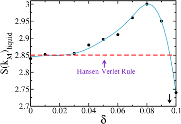
Figure 2: The variation of first peak maximum of the liquid structure factor with different polydispersity indices ${\delta}$. The structure factor of the liquid phase for different ${\delta}$ is calculated for the corresponding co-existence volume fraction ${\varphi}$ at temperature $T^{*}=1$. The red dotted line signifies the predicted value obtained from Hansen-Verlet rule of crystallization. Please note that black arrow shows the structural transformation at polydispersity ${\delta}$ =0.095 predicted by structure factor analysis that agrees well with all other analyses (inherent structure, free energy, Lindemann criterion) presented here.

IV.2 Lindemann criterion in melting of polydisperse system

This phenomenological criterion was put forward by Lindemann in 1910. The idea behind the theory was the observation that the average amplitude of thermal vibrations increases with increasing temperature Lindemann (1910). Melting initiates when the amplitude of vibration becomes large enough for adjacent atoms to partly occupy the same space. The Lindemann criterion states that melting is expected when the root mean square vibration amplitude exceeds a threshold value. Hence one can write

$$L=\frac{\sqrt{\left\langle\mathop{\overrightarrow{r}}\nolimits_{i}^{2}\right\rangle}}{a},$$ (10)

where $L$ is the Lindemann parameter for the associated polydisperse system and ${a}$ is the mean distance between the particles. This threshold value of Lindemann constant is $L\approx 0.1$for melting of crystals Nelson (2002) of point-like particles in three dimensions, but it may vary between 0.05 and 0.20 depending on different factors like nature of inter particle interactions, crystal structure, and magnitude of quantum effects.

Fig. 3 shows the variation of Lindemann parameter ($L$) with respect to polydispersity indices ($\delta$) for three different temperatures $T^{*}$= 1.0, 0.8 and 0.5 for a constant volume fraction $\Phi$ = 0.58. The plot shows that the value of $L$ increases with the increase of $\delta$. For temperatures $T^{*}$=1.0, 0.8 and 0.5, $L$ crosses the threshold value 0.1 at $\delta$ = 0.09, 0.10 and 0.13 respectively. This signifies the onset of melting processes at $\delta$ = 0.09, 0.10 and 0.13 for $T^{*}$=1.0, 0.8 and 0.5 respectively in the Lennard-Jones polydisperse solid, when the amplitude of the root mean square vibration exceeds a threshold value taken as $L$ = 0.1.

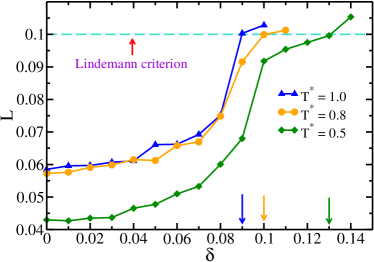
Figure 3: Variation of Lindemann parameter ($L$) with respect to polydispersity indices (${\delta}$). Please note that with increase in polydispersity, the value of $L$ also increases and for temperature $T^{*}=1.0$, the value of $L$ crosses the threshold value 0.1 at ${\delta}$ = 0.09 (as indicated by blue arrow), for $T^{*}=0.8$, $L$ crosses the threshold value at ${\delta}$ = 0.10 (as indicated by orange arrow) and for $T^{*}=0.5$, $L$ crosses the threshold value at ${\delta}$ = 0.13 (as indicated by green arrow). Note that blue, orange and green arrows signify the onset of melting process at ${\delta}$ = 0.09, 0.10 and 0.13 corresponding to the temperatures $T^{*}$= 1.0, 0.8 and 0.5 respectively.

IV.3 Prediction of transition polydispersity from inherent structure analysis

IV.3.1 Correlation between transition polydispersity and average inherent structure energy

In polydisperse hard sphere fluids attractive interaction potential is not taken into account. Hard sphere system shows reentrant melting of the solid and also above a threshold value of polydispersity (known as terminal polydispersity) hard sphere does not form solid phase under any condition. On the other hand, for LJ fluid model system, the attractive potential is taken into account and hence it is interesting to study the influence of the attractive part of potential on the terminal polydispersity.

As shown in Fig. 4, the average IS energy is computed with increase in polydispersity for different volume fractions $\Phi$ = 0.48, 0.52, 0.58, 0.64, 0.70 at constant temperature $T^{*}=1.0$. The average IS energy increases almost quadratically with polydispersity up to a polydispersity index at which structural transition takes place. This polydispersity index is known as “transition polydispersity,” beyond which the crystalline solid phase is no longer stable and amorphous phase exists. We achieve the transition polydispersity $\left(\delta_{t}\right)$ for different volume fractions using IS analysis. The crossover of the two slopes corresponding to each $\Phi$ signifies the transition polydispersity where the structural transition from FCC to amorphous state takes place. Table 1 shows the transition polydispersities $\left(\delta_{t}\right)$ for the melting transition of the Lennard-Jones polydisperse system corresponding to different values of volume fractions and for constant temperature $T*=1.0$.

Table 1: Numerical values of transition polydispersity for the melting transition of Lennard-Jones polydisperse systems. The first column represents the volume fraction $\Phi$ and second column represents the transition polydispersity ($\delta_{t}$) correspond to each $\Phi$.

${\Phi}$	$\mathbf{\delta}_{t}$
0.48	0.02
0.52	0.07
0.58	0.09
0.64	0.10
0.70	0.11

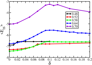
Figure 4: Variation of average IS energy with respect to polydispersity index at constant temperature $T^{*}$ = 1.0 for different volume fractions ${\Phi}$ = 0.48, 0.52, 0.58, 0.64, 0.70. The average IS energy increases with increase in polydispersity until transition polydispersity, when the dependence changes sharply. Note that at low volume fraction ${\Phi}$, the transition occurs at lower value of ${\delta}$ and at higher ${\Phi}$, solid phase is stable up to higher ${\delta}$ value.

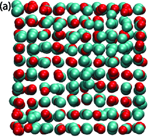
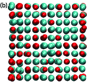
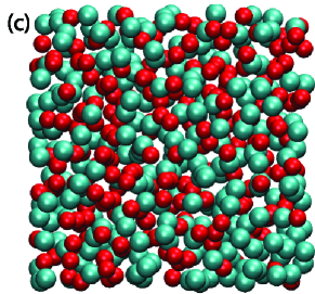
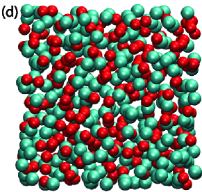
Figure 5: (Color online) Snapshots showing the spatial positions of small particle in red (dark gray) and big particle in cyan (light gray) color in the parent structure along with its corresponding inherent structure at different polydispersity indices. Please note that the parent structure is at temperature T*=1 and ${\Phi}$ = 0.58. (a) Parent structure corresponds to the polydispersity index 0.08. Note the crystal-like structure of the parent polydisperse system (b) Inherent structure at ${\delta}$ = 0.08 shows the more structured formation than the corresponding parent structure (c) Snapshot shows parent structure at ${\delta}$ = 0.09 and (d) corresponding inherent structure at ${\delta}$ = 0.09. Note that fig. 5(c, d) depict amorphous/glass like formation in the parent and inherent structure at ${\delta}$ = 0.09.

Difference in the polydispersity index ($\delta$) dependence of the inherent structure (IS) energy in the crystalline solid and in the amorphous phase is understandable in terms of the theory of elasticity in solids Landau and Lifshitz (1981). In the presence of a strain field, the free energy can be written as,

$$F=F_{0}+\frac{1}{2}\lambda u^{2}_{ii}+\mu u_{ik}^{2},$$ (11)

where $\lambda$ and $\mu$ are called Lamé coefficients.

$$K=\lambda+\frac{2}{3}\mu.$$ (12)

Here $K$ and $\mu$are bulk modulus and modulus of rigidity respectively.

Now in the crystalline solid, polydispersity introduces strain field $u_{ik}$which is randomly distributed in the solid and strongly dependent on $\delta$. As $\delta$ increases, strain field also increases. The quantitative estimate in the free energy can be achieved from the density-functional theory of elasticity Jarić and Mohanty (1988); Lipkin et al. (1985). On the other hand, the particles in the amorphous phase can undergo rearrangements to reduce the strain which explains the weak dependence of the IS energy with $\delta$ in the amorphous phase. This allows us to estimate quantitatively the criterion of transition from IS analysis. Another point to notice is that the change of the IS energy at the cross over depends both on temperature and volume fraction. As the volume fraction is lowered, the effect of the strain field on the IS energy of the solid decreases. This describes the reason of different transition polydispersity indices $\left(\delta_{t}\right)$for different volume fractions.

IV.3.2 Structural patterns of parent structure and corresponding inherent structure at different polydispersity indices

The transition polydispersity for the melting transition of the Lennard-Jones polydisperse system needs further exploration. We study the structural aspects at different polydispersity indices. We categorize the particles into two sub ensembles; particles with diameter less than 1.0 are termed as small particle and rest of the particles as big particle. In Fig. 5 we represent the snapshots showing the spatial positions of small particle in red and big particle in cyan color in the parent structure along with its corresponding inherent structure at different polydispersity indices. The snapshots of the parent liquid have been taken at reduced temperature $T^{*}=1.0$, and volume fraction $\Phi$ = 0.58. Fig. 5 shows an instantaneous parent structure at $\delta$ = 0.08 and Fig. 5 shows its corresponding inherent structure while Figs. 5, 5 depict molecular arrangements for the parent structure at $\delta$ = 0.09 and its inherent structure respectively. Fig. 5 and  5 reveal the crystal-like arrangement of the particles in both parent and inherent structure respectively. Fig. 5 and 5 show instantaneous parent structure and corresponding inherent structure at $\delta$ = 0.09 which seem to be almost homogeneous. These four snapshots show structural transition of the present L-J polydisperse system when the system enters from $\delta$ = 0.08 to $\delta$ = 0.09.

IV.4 Relationship among scaled order parameter ($\lambda_{\vec{G}}$) in the scaled phase diagram and coexistence densities of solid and liquid

With the increase in polydispersity indices, the coexistence density of the solid $(\rho_{s}^{*})$approaches that of the liquid $(\rho_{l}^{*})$ and the value of the direct correlation function at its first peak decreases. Hence, the value of the order parameter ($\lambda_{\vec{G}}$) in the scaled phase diagram decreases with the increase in coexistence density of solid $(\rho_{s}^{*})$ and that of liquid $(\rho_{l}^{*})$ as shown in Fig. 6.

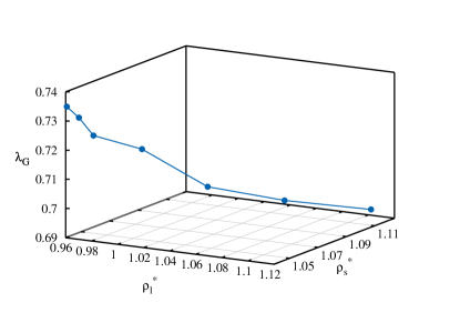
Figure 6: Variation of scaled order parameter ($\lambda_{\vec{G}}$) in the phase diagram with coexistence density of solid $(\rho_{s}^{*})$ and liquid $(\rho_{l}^{*})$. Note that the value of the scaled order parameter ($\lambda_{\vec{G}}$) decreases as both the coexistence density of solid $(\rho_{s})$ and that of liquid $(\rho_{l})$ increase.

That is, in the phase diagram given by Fig. 1, one moves toward left along the upper branch. Since no transition is possible beyond the spinodal point, this point can be identified with the instability point of Lindemann melting criteria.

IV.5 Discussion

In our present study we are interested in melting of the solid due to increase in polydispersity, as elaborated by the IS analysis. As the polydispersity increases, several things occur that determine the position of the coexistence. First, the density of the solid at coexistence approaches that of the liquid. Also, the crystalline order of the solid decreases progressively which is reflected in the lower value of the order parameters. Thus, the value of the ordinate (that gives scaled order parameter,$\psi_{\vec{G}}$) in the scaled phase diagram (the upper solid line) decreases as polydispersity increases. At the same time, value of the abscissa also decreases because the density of the solid approaches that of the liquid and the value of the direct correlation function at its first peak decreases. All these lead the system towards the first terminal point which can thus be identified as the limit of stability of the polydisperse solid with respect to the liquid. The results obtained for the melting transition parameters of the Lennard-Jones polydisperse solids are shown in Table 2. Interestingly, the value of the polydispersity index (for a constant volume fraction) at which melting is predicted agrees well with Lindemann criteria of atom displacement.

In order to explore the mechanical stability of a metastable solid through inherent structure analysis, the potential energy of the solid must be a minimum. We find that beyond a given polydispersity index (at a constant volume fraction) no such minimum, indicating that amorphous state represents the true ground state of the system.

From the liquid side, we can get an estimate of the transfer of stability from liquid to solid state by (a) Ramakrishnan and Yussouff theory  Ramakrishnan and Yussouff (1979) (b) empirical Hansen-Verlet rule Hansen and Verlet (1969). Both again give values of liquid and solid density those are in agreement with inherent structure analysis and integral equation based theoretical analysis of liquid-solid transition.

Table 2: Comparison of values of melting parameters. The first column represents value of polydispersity index (${\delta}$) and second column represents corresponding critical pressure $(P^{*})$ at coexistence of solid and liquid phases. Third and fourth columns represent critical density of solid $(\rho_{s}^{*})$ and its volume fraction $(\phi_{S})$ respectively. Fifth and sixth columns represent critical density of liquid $(\rho_{l}^{*})$ and its volume fraction $(\phi_{l})$ respectively. The value of $(\phi_{0})$ represents fractional density change on melting transition. The value of $S\left(k_{M}\right)_{L}$ shows the value of the liquid structure factor at the first peak. In the last column $\lambda_{\vec{G}}$ represents the value of the scaled order parameter.

${\mathbf{\delta}}$	$P^{*}$	$\rho_{s}^{*}$	$\phi_{S}$	$\rho_{l}^{*}$	$\phi_{l}$	$\phi_{0}$	$S\left(k_{M}\right)_{L}$	$\lambda_{\vec{G}}$
0.0	6.58	1.039	0.544	0.961	0.503	0.075	2.839	0.735
0.01	6.73	1.042	0.546	0.967	0.507	0.072	2.852	0.731
0.03	7.10	1.044	0.547	0.976	0.511	0.065	2.855	0.725
0.04	8.28	1.058	0.554	0.998	0.523	0.058	2.879	0.719
0.06	10.40	1.074	0.563	1.031	0.540	0.040	2.911	0.705
0.07	12.97	1.097	0.575	1.065	0.558	0.029	2.961	0.698
0.08	16.30	1.124	0.588	1.102	0.577	0.019	3.001	0.692
0.09	-	-		-	-		2.949	-
0.10	-	-		-	-		2.740	-

We note that if we apply Ramakrishnan-Yussouff theory to find the freezing density with an effective direct correlation function, then we obtain values that are close to the values given in Table 2. As evident from Table 2 (also indicated in Fig. 1), with increasing polydispersity index $\delta$, density of liquid at solid- liquid transition increases. This leads to an increase in the first peak of the liquid structure factor, $S(k)_{Liquid}$. At the same time, value of the scaled order parameter ($\lambda_{\vec{G}}$) decreases because the density of the co-existence solid increases. This is the direct consequence of the sharp fall in the fractional density change ($\phi_{0}$) on melting-freezing. As $\delta$ increases, both of the changes in $\lambda_{\vec{G}}$ and $\psi_{\vec{G}}$ values drive the system to the turning point/spinodal point (as shown in Fig. 1). Below the particular value of $\lambda_{\vec{G}}$ at spinodal point, no liquid-solid transition is possible.

V Conclusion

The terminal polydispersity has not been studied earlier in the Lennard-Jones polydisperse system using non-linear integral equation theories of freezing. We discuss how certain features of the scaled phase diagram may be used to explain the terminal polydispersity in polydisperse system. This analysis implies that at high polydispersity, the equality of thermodynamic potential between solid and liquid phases can no longer be established. The liquid state has lower chemical potential and the solid phase is not possible beyond certain polydispersity. This is manifested in the absence of any solution of the non-linear integral equations. The same feature is reflected in the inherent structure analysis - no crystalline solid is obtained in the inherent structure beyond the terminal polydispersity. The amorphous state is the global minimum in the potential energy surface.