A new relation between the zero of $A_{FB}$ in $B^{0}\to K^{*}\mu^{+}\mu^{-}$ and the anomaly in $P_{5}^{\prime}$

Abstract

We present two exact relations, valid for any dilepton invariant mass region (large and low-recoil) and independent of any effective Hamiltonian computation, between the observables $P_{i}$ and $P_{i}^{CP}$ of the angular distribution of the 4-body decay $B\to K^{*}(\to K\pi)l^{+}l^{-}$. These relations emerge out of the symmetries of the angular distribution. We discuss the implications of these relations under the (testable) hypotheses of no scalar or tensor contributions and no New Physics weak phases in the Wilson coefficients. Under these hypotheses there is a direct relation among the observables $P_{1}$,$P_{2}$ and $P_{4,5}^{\prime}$. This can be used as an independent consistency test of the measurements of the angular observables. Alternatively, these relations can be applied directly in the fit to data, reducing the number of free parameters in the fit. This opens up the possibility to perform a full angular fit of the observables with existing datasets. An important consequence of the found relations is that a priori two different measurements, namely the measured position of the zero ($q_{0}^{2}$) of the forward-backward asymmetry $A_{FB}$ and the value of $P_{5}^{\prime}$ evaluated at this same point, are related by $P_{4}^{2}(q_{0}^{2})+P_{5}^{2}(q_{0}^{2})=1$. Under the hypotheses of real Wilson coefficients and $P_{4}^{\prime}$ being SM-like, we show that the higher the position of $q_{0}^{2}$ the smaller should be the value of $P_{5}^{\prime}$ evaluated at the same point. A precise determination of the position of the zero of $A_{FB}$ together with a measurement of $P_{4}^{\prime}$ (and $P_{1}$) at this position can be used as an independent experimental test of the anomaly in $P_{5}^{\prime}$. We also point out the existence of upper and lower bounds for $P_{1}$, namely $P_{5}^{\prime 2}-1\leq P_{1}\leq 1-P_{4}^{\prime 2}$, which constraints the physical region of the observables.

PACS numbers

13.25.Hw, 11.30.Er, 11.30.Hv

LHCb has performed LHCbpaper1 ; LHCbpaper a measurement of the form factor independent (so called clean) observables kruger ; complete in the decay $B^{0}\to K^{*}(\to K\pi)\mu^{+}\mu^{-}$. These measurements, performed in six independent bins of the dimuon invariant mass squared ($q^{2}$), were based on a dataset corresponding to an integrated luminosity of 1fb^-1. Soon after, the first phenomenological analysis of the full set of measurements, at large and low recoil, appeared thefirst . This analysis had two main conclusions. Firstly, it was emphasized that besides a striking 4$\sigma$ deviation in one bin of one observable a set of other less significant deviations (below 3$\sigma$) were also present in a coherent pattern. Secondly, this pattern pointed to the Wilson coefficient of the semileptonic operator $O_{9}$ as the main responsible, without excluding possible small contributions from Wilson coefficients of other operators. The connection among those different tensions was shown in Ref. thefirst at the level of operators of an effective Hamiltonian within a specific framework qcdf1 to compute QCD corrections. Other analyses that used different approaches straub ; danny ; lat were also presented, including implications for possible NP models uli ; buras ; datta ; nazila .

In the present paper we show that the connection between the discrepancy in the observables $P_{5}^{\prime}$ and $P_{2}$ is deeper and can be proved at a more fundamental level, i.e. using the symmetries of the angular distribution. We point towards a completely new way to test the anomaly in $P_{5}^{\prime}$ via a measurement of the zero in the forward-backward asymmetry ($q^{2}_{0}$) as a key observable. At present LHCb measured the zero to be at $q_{0}^{2}=4.9\pm 0.9$ GeV²LHCbpaper1 and our SM prediction is $q_{0}^{2}=3.95\pm 0.38$ GeV². The results presented in this paper connect the values of $P_{5}^{\prime}$, $P_{4}^{\prime}$ and $P_{1}$ when evaluated at $q_{0}^{2}$.

The structure of this paper is the following: in Section I we recall the symmetry relations between the angular observables and we show how this leads to an exact relation between the clean observables. In this section, we obtain three results: first, a relation between $P_{2}$ and the other $P_{i}$ (and $P_{i}^{(CP)}$) observables, second, a new constraint for $P_{1}$ and third, a relation between the values of different clean observables evaluated at $q_{0}^{2}$ (the zero of $P_{2}$ or $A_{FB}$). In Section II we restrict those relations to the case of no New Physics (NP) phases in the Wilson coefficients and all relations simplify considerably. Then we apply these results to $q^{2}$ averaged observables. In Section III we show the implications for future analyses imposing the obtained relations in fits to data.

I Exact symmetry relation

The description of the angular distribution of the decay $B^{0}\to K^{*}(\to K\pi)\mu^{+}\mu^{-}$, if lepton masses and scalar contributions are neglected, is completely given by a basis of eight observables optimizing

$${\cal O}=\{P_{1},P_{2},P_{3},P_{4}^{\prime},P_{5}^{\prime},P_{6}^{\prime},A_{FB},d\Gamma/dq^{2}\}$$ (1)

If lepton masses are considered, two extra observables ($M_{1,2}$ or ${\tilde{F}_{L,T}}$) have to be added. See complete ; swave ; optimizing for definitions. In addition the observable $P_{8}^{\prime}$ can be used to either substitute one of the $P_{i}$ observables (for instance $P_{3}$) or express it in terms of all other observables of the basis. The $P_{i}$ observables are related to the coefficients ($J_{i}$) of the angular distribution by

$$({J_{2s}}+{\bar{J}_{2s}}) = \frac{1}{4}N_{1},\quad({J_{2c}}+{\bar{J}_{2c}})=-N_{2},\,\,$$

$${J_{3}}+{\bar{J}_{3}} = \frac{1}{2}{P_{1}}N_{1},\quad{J_{4}}+{\bar{J}_{4}}=\frac{1}{2}{P_{4}^{\prime}}N_{3},$$

$${J_{5}}+{\bar{J}_{5}} = {P_{5}^{\prime}}N_{3},\quad{J_{6s}}+{\bar{J}_{6s}}=2{P_{2}}N_{1},$$

$${J_{7}}+{\bar{J}_{7}} = -{P_{6}^{\prime}}N_{3},\quad{J_{8}}+{\bar{J}_{8}}=-\frac{1}{2}{P_{8}^{\prime}}N_{3},$$

$${J_{9}}+{\bar{J}_{9}} = -{P_{3}}N_{1}$$ (2)

where $N_{1,2}=\beta^{2}F_{T,L}\frac{d\Gamma}{dq^{2}}$ and $N_{3}=\beta^{2}\sqrt{F_{T}F_{L}}\frac{d\Gamma}{dq^{2}}$ with $\beta=\sqrt{1-4m_{l}^{2}/q^{2}}$. Notice that these expressions are all taken proportional to $\beta^{2}$ to match the standard definition of the $P_{i}$ given in optimizing . The set of $P_{i}^{CP}$, $F_{L,T}^{CP}$ observables are defined using the same Eqs.(2) substituting $J_{i}+{\bar{J}_{i}}\to J_{i}-{\bar{J}_{i}}$ (see optimizing for detailed definitions). The coefficients $J_{i}$ are bilinear functions of the transversity amplitudes $A_{0}^{L,R},A_{\parallel}^{L,R},A_{\perp}^{L,R}$ and the observables $P_{i}^{(\prime)}$ are ratios of those bilinears.

Sometime ago, one of us identified four symmetry transformations among the transversity amplitudes that leave the angular distribution invariant ulrik2 . Working under the hypothesis of no scalar contributions one can easily solve the transversity amplitudes in terms of the $J_{i}$ using three of those symmetries (see Sec. 3.3 of ulrik2 ). The remaining fourth symmetry showed up as a relation between the phases of two of the transversity amplitudes. The following non-trivial consistency relationship between the coefficients of the distribution emerges as a byproduct of imposing that the modulus of this relative phase should be one ulrik2 ; complete

$$J_{2c}=+4\,\frac{\beta_{\ell}^{2}J_{6s}(J_{4}J_{5}+J_{7}J_{8})+J_{9}(\beta_{\ell}^{2}J_{5}J_{7}-4J_{4}J_{8})}{16J_{2s}^{2}-\left(4J_{3}^{2}+\beta_{\ell}^{2}J_{6s}^{2}+4J_{9}^{2}\right)}$$ (3)

$$-2\,\frac{(2J_{2s}+J_{3})\left(4J_{4}^{2}+\beta_{\ell}^{2}J_{7}^{2}\right)+(2J_{2s}-J_{3})\left(\beta_{\ell}^{2}J_{5}^{2}+4J_{8}^{2}\right)}{16J_{2s}^{2}-\left(4J_{3}^{2}+\beta_{\ell}^{2}J_{6s}^{2}+4J_{9}^{2}\right)}$$

An identical relation follows for the coefficients ${\bar{J}}_{i}$, by simply CP-conjugating Eq.(3).

By using Eq.(3) and Eqs.(2) it is possible to write an expression for $P_{2}$ in terms of the other $P_{i}^{(\prime)}$ observables. More precisely, one obtains two relations, one between the observables ${\bar{P}_{i}}=P_{i}+P_{i}^{CP}$ and a second relation between the observables ${\hat{P}_{i}}=P_{i}-P_{i}^{CP}$. The first relation is given by

$${\bar{P}_{2}}=+\frac{1}{2{\bar{k}_{1}}}\bigg{[}({\bar{P}_{4}^{\prime}}{\bar{P}_{5}^{\prime}}+\delta_{1})+\frac{1}{\beta}\sqrt{(-1+{\bar{P}_{1}}+{\bar{P}_{4}^{\prime 2}})(-1-{\bar{P}_{1}}+\beta^{2}{\bar{P}_{5}^{\prime 2}})+\delta_{2}+\delta_{3}{\bar{P}_{1}}+\delta_{4}{\bar{P}_{1}}^{2}}\bigg{]}$$ (4)

where $\delta_{i}$ are defined in Table 1 and where ${\bar{k}_{1}}=1+{F_{L}^{CP}}/{F_{L}}$ and ${\bar{k}_{2}}=1+F_{T}^{CP}/F_{T}$. Notice that the existence of this relation is not in contradiction with the fact that the $P_{i}$ define a basis because Eq.(4) involves 7 of the $P_{i}$ (and $P_{i}^{CP}$) but only 6 of them are independent. An identical expression for the ${\hat{P}_{i}}$ observables is obtained from Eq.(4) substituting ${\bar{P}_{i}}\to{\hat{P}_{i}}$ (also inside the $\delta_{i}$) and ${\bar{k}_{i}}\to{\hat{k}_{i}}$, where ${\hat{k}_{1}}=1-{F_{L}^{CP}}/{F_{L}}$ and ${\hat{k}_{2}}=1-F_{T}^{CP}/F_{T}$.

Table 1: Definitions of $\delta$ functions in terms of $P_{i}$ and $P_{i}^{CP}$ observables.

$\delta_{1}={\bar{P}_{6}^{\prime}}{\bar{P}_{8}^{\prime}}\quad\quad\quad\quad\delta_{4}=1-{\bar{k}_{1}}^{2}\quad\quad\quad\quad\delta_{3}=(1-{\bar{k}_{1}}){\bar{P}_{4}^{\prime 2}}+\beta^{2}[(-1+{\bar{k}_{1}}){\bar{P}_{5}^{\prime 2}}-{\bar{k}_{1}}{\bar{P}_{6}^{\prime 2}}]+{\bar{k}_{1}}{\bar{P}_{8}^{\prime 2}}$
$\delta_{2}=-1+{\bar{k}_{1}}^{2}{\bar{k}_{2}}^{2}+(1-{\bar{k}_{1}}{\bar{k}_{2}})({\bar{P}_{4}^{\prime 2}}+\beta^{2}{\bar{P}_{5}^{\prime 2}})-4{\bar{k}_{1}^{2}}{\bar{P}_{3}^{2}}+\beta^{2}{\bar{P}_{6}^{\prime}}{\bar{P}_{8}^{\prime}}(2{\bar{P}_{4}^{\prime}}{\bar{P}_{5}^{\prime}}+{\bar{P}_{6}^{\prime}}{\bar{P}_{8}^{\prime}})+{\bar{k}_{1}}[\beta^{2}{\bar{P}_{6}^{\prime}}(4{\bar{P}_{3}}{\bar{P}_{5}^{\prime}}-{\bar{k}_{2}}{\bar{P}_{6}^{\prime}})-{\bar{P}_{8}^{\prime}}(4{\bar{P}_{3}}{\bar{P}_{4}^{\prime}}+{\bar{k}_{2}}{\bar{P}_{8}^{\prime}})]$

Eq.(4) is an exact relation valid for any value of $q^{2}$. We take ”+” sign in front of square root by consistency with SM, at low-recoil both solutions ($\pm$) tend to converge at the very endpoint.

From Eq.(4) imposing that the argument of the square root is positive, one obtains the following restriction on $\bar{P}_{1}$

$$u-\sqrt{u^{2}+v}\leq{\bar{P}_{1}}\leq u+\sqrt{u^{2}+v}$$ (5)

with

$$u = \frac{1}{2(1-\delta_{4})}[(-1+\beta^{2}{\bar{P}_{5}^{\prime 2}})-(-1+{\bar{P}_{4}^{\prime 2}})+\delta_{3}]$$

$$v = \frac{1}{1-\delta_{4}}[(-1+{\bar{P}_{4}^{\prime 2}})(-1+\beta^{2}{\bar{P}_{5}^{\prime 2}})+\delta_{2}]$$ (6)

Another important consequence originates from evaluating Eq.(4) at $q_{0}^{2}$. The following relation emerges among the different observables:

$$[(1+{\bar{P}_{1}}){\bar{P}_{4}^{\prime 2}}+\beta^{2}(1-{\bar{P}_{1}}){\bar{P}_{5}^{\prime 2}}+{\bar{P}_{1}}^{2}+\omega]_{q^{2}=q_{0}^{2}}=1\quad$$ (7)

where $\omega$ is strongly suppressed and it is defined by

$$\omega=\beta^{2}\delta_{1}(\delta_{1}+2{\bar{P}_{4}^{\prime}}{\bar{P}_{5}^{\prime}})-{\bar{P}_{1}}(\delta_{3}+\delta_{4}{\bar{P}_{1}})-\delta_{2}$$ (8)

Let us remark that all expressions up to this point are exact, except for the assumptions of no scalar/tensor contributions. In the following we will work within one extra NP hypothesis and one approximation that simplifies considerably the analysis.

II Constrained New Physics and Real Wilson coefficients

We will assume now that NP does not introduce any new weak phase on Wilson coefficients. This hypothesis implies that $P_{i}^{CP}\sim 0$ and $F_{L}^{CP}\sim 0$, including the small SM contribution. Consequently, ${\bar{P}_{i}}\to P_{i}$, ${\hat{P}_{i}}\to P_{i}$ and the two Eqs.(4) become a single equation. This hypothesis can be tested by measuring the $P_{i}^{CP}$. Moreover, taking into account that $J_{7,8,9}$ are functions of ${\rm Im}A_{i}A_{j}={\rm Im}A_{i}{\rm Re}A_{j}+{\rm Im}A_{j}{\rm Re}A_{i}$ one can easily see that while $\bar{P}_{3}$ and $\bar{P}_{6,8}^{\prime}$ are ${\cal O}({\rm Im}A_{i})$ the $\delta_{i}$ are further suppressed $\delta_{i}\sim{\cal O}(({\rm Im}A_{i})^{2},1-{\bar{k}_{1}},1-{\hat{k}_{1}})$.

	$\delta_{1}$	$\delta_{2}$	$\delta_{3}$	$\delta_{4}$
$|SM|$	$\lesssim 0.01$	$\lesssim 0.03$	$\lesssim 0.01$	$\lesssim 0.01$
NP	$[-0.03,0.01]$	$[-0.09,0.01]$	$[-0.04,0.04]$	$[-0.03,0.02]$

Table 2: First line corresponds to the $|\delta_{i}|$ bounds in the SM while second one is the range for $\delta_{i}$ in presence of NP.

In the following we cross check this by using an effective Hamiltonian approach in the SM and in presence of NP.

Even if all the equations discussed up to now are valid for all $q^{2}$ values, we will focus mainly on the most interesting region $1\leq q^{2}\leq 6$ GeV². In this region the observables ${\bar{P}_{3}}$, ${\bar{P}_{6,8}^{\prime}}$ are approximately bounded in the SM to be $|\bar{P}_{3}|\lesssim 5\times 10^{-3}$, $|{\bar{P}_{6}^{\prime}}|\lesssim 10^{-1}$, $|\bar{P}_{8}^{\prime}|\lesssim 10^{-1}$. Given that these observables enter quadratically inside the $\delta_{i}$, the size of the $\delta_{i}$ is negligible. The bounds on the $|\delta_{i}|$, obtained varying $q^{2}$ in the 1 to 6 GeV² region, are given in Table 2 and the bounds on the relevant combinations entering Eq.(4) and Eq.(7) of previous section are $|\delta_{2}+\delta_{3}\bar{P}_{1}+\delta_{4}{\bar{P}_{1}}^{2}|\lesssim 0.03$ and $|\omega|\lesssim 0.01$. The $\omega$ term is evaluated around the $q_{0}^{2SM}$ in a 1 GeV² bin size.

Then, to a very good approximation, Eq.(4) taking $\delta_{i}\to 0$ (and ${\bar{k}}_{i}\to 1$) simplifies to

$$P_{2}=\frac{1}{2}\left[P_{4}^{\prime}P_{5}^{\prime}+\frac{1}{\beta}\sqrt{(-1+P_{1}+P_{4}^{\prime 2})(-1-P_{1}+\beta^{2}P_{5}^{\prime 2})}\right]$$ (9)

As Fig.1 (left) shows, this equation is fulfilled to excellent accuracy in the SM.

We repeated the analysis of the bounds on $\delta_{i}$ allowing for the presence of NP in the Wilson coefficients of the dipole and semileptonic operators. We define from now on by NP a range for the Wilson coefficients according to the (enlarged) pattern found in thefirst

$$-0.1 \leq C_{7}^{NP}\leq 0.1,\,-2\leq C_{9}^{NP}\leq 0,\,-1\leq C_{10}^{NP}\leq 1\hfill$$

$$-0.1 \leq C_{7}^{\prime}\leq 0.1,\quad-2\leq C_{9}^{\prime}\leq 2,\quad-1\leq C_{10}^{\prime}\leq 1\quad\,\,\,\,$$ (10)

Then, the corresponding range of maximal variation of the $\delta_{i}$ terms allowing for NP is given in Table 2.

The range for the combination of $\delta_{i}$ terms entering Eq.(4) that we obtain in the presence of NP is

$$-0.07\lesssim\delta_{2}+\delta_{3}\bar{P}_{1}+\delta_{4}{\bar{P}_{1}}^{2}\lesssim 0.01$$ (11)

This shows that Eq.(4) is an excellent approximation, as Fig.1 (left) illustrates, also in presence of NP.

Table 3: Comparison between $P_{2}$ evaluated in bins and $P_{2}$ obtained from Eq.(9) assuming its validity in binned form. First row is the difference between the exact result and the result obtained using the relation Eq.(9) in the SM, second and third row are the ranges allowing for New Physics as defined in Eq.(10). Last row is the corresponding comparison for one point of NP ($C_{9}^{\rm NP}=-1.5$). Notice that for small bin size the correction is tiny.

Point	[0.1-2]∗	[2-4.3]	[4.3-8.68]	[1-6]∗	[1-2]	[2-3]	[3-4]	[4-5]	[5-6]
$\rm\Delta^{SM}_{exact-relation}$	$-0.14$	$-0.06$	$-0.03$	$-0.21$	$-0.02$	$-0.02$	$-0.01$	$-0.01$	$-0.01$
${\rm\Delta^{NP}_{exact-relation}}^{upper}$	$-0.07$	$-0.02$	$-0.02$	$-0.08$	$+0.00$	$+0.00$	$+0.00$	$+0.00$	$+0.01$
${\rm\Delta^{NP}_{exact-relation}}^{down}$	$-0.23$	$-0.10$	$-0.09$	$-0.28$	$-0.07$	$-0.04$	$-0.03$	$-0.02$	$-0.04$
${\rm\Delta^{C_{9}^{NP}=-1.5}_{exact-relation}}$	$-0.11$	$-0.04$	$-0.04$	$-0.16$	$-0.01$	$-0.01$	$-0.01$	$-0.01$	$-0.01$

The bounds given by Eq.(5) also simplify to

$$P_{5}^{\prime 2}-1\leq P_{1}\leq 1-P_{4}^{\prime 2}$$ (12)

While this equation is approximate for $\bar{P}_{1}$ it turns out to be exact for $P_{1}$, since it can be also obtained from the simple bound $|P_{4}|=|P_{4}^{\prime}|/\sqrt{1-P_{1}}\leq 1$ coming from the geometrical interpretation of $P_{4}$ (see Eq.(16) in complete ). From $|P_{5}|=|P_{5}^{\prime}|/\sqrt{1+P_{1}}\leq 1$ one gets the lower bound that is particularly important at low recoil. Also $|P_{4}^{\prime}P_{5}^{\prime}|\leq 1$ follows.

The evaluation of $\omega$ in presence of NP around the position of the zero of $A_{FB}$ for each NP point gives $-0.01\lesssim\omega\lesssim 0.07$. The smallness of this quantity leads to the last important result, namely the condition Eq.(7) between the observables evaluated at $q_{0}^{2}$ turns out to be

$$[P_{4}^{2}+P_{5}^{2}]|_{q^{2}=q_{0}^{2}}=1$$ (13)

assuming $P_{1}^{2}(q_{0}^{2})\neq 1$, or in terms of the more interesting $P_{4,5}^{\prime}$ observables:

$$[P_{4}^{\prime 2}+P_{5}^{\prime 2}]_{q^{2}=q_{0}^{2}}=1-\eta(q_{0}^{2})$$ (14)

where

$$\eta(q_{0}^{2})=[P_{1}^{2}+P_{1}(P_{4}^{\prime 2}-P_{5}^{\prime 2})]_{q^{2}=q_{0}^{2}}$$

From the geometrical interpretation of the observables $P_{4,5}$ given in Eq.(16-17) of Ref. complete it is evident that they fulfill $|P_{4,5}|\leq 1$. Moreover, in the SM for $q^{2}\gg q_{0}^{2SM}$ both $|P_{4,5}|$ tend to one, while at $q_{0}^{2SM}=3.95$ GeV² they fulfill Eq.(13) to an excellent accuracy. In presence of NP, if the zero of $A_{FB}$ appears at a higher position and $P_{4}$ is SM-like, given that $P_{4}$ tends to 1 for $q^{2}>q_{0}^{2}$, Eq.(13) implies that the higher the position of $q^{2}_{0}$ the closer to zero the value of $P_{5}$ at this point should be. The same arguments apply for $P_{4,5}^{\prime}$ if $q_{0}^{2}>q_{0}^{2SM}$ (notice that data prefers a $P_{1}$ positive in the region of the third bin but the bound coming from $P_{4}^{\prime}$ Eq.(12) constrain $P_{1}$ to be small in that region), consequently, $\eta(q_{0}^{2})$ is expected to be small and because of that also the value of $P_{5}^{\prime}$ evaluated at $q_{0}^{2}$ would tend to a smaller value as present data seem to hint.

II.1 Averaging over $q^{2}$

All previous equations are strictly valid only for a fixed $q^{2}$ value. However, the measurements are performed as averages in bins of $q^{2}$. Since Eq.(9) is not linear in the observables, it is in general not valid when averaging over $q^{2}$ regions. The only circumstance that would justify the use of this equation when $P_{i}\to\langle P_{i}\rangle$, which we will refer to as binned form of the equation, would be that all observables were approximately constant inside the bin. Consequently, this approximation tends to be more valid the smaller the bin size.

In Table 3 we evaluate the difference between the exact binned result, averaging over $q^{2}$, and the one obtained using Eq.(9) assuming its validity for $q^{2}$ average observables, in three cases: a) SM, b) in presence of NP and c) at the best fit point $C_{9}^{\rm NP}=-1.5$. In this way we estimate (now using an effective Hamiltonian approach) the maximal shift

$$\langle P_{2}\rangle\to\langle P_{2}\rangle+{\Delta^{\rm X}_{\rm exact-relation}}$$

due to the $q^{2}$ binning, where $X={\rm SM},{\rm NP},C_{9}^{\rm NP}=-1.5$. We compute it using the binning scheme adopted by the experiments LHCbpaper1 ; LHCbpaper ; CMSKstmm ; Aubert:2008bi ; Wei:2009zv ; Aaltonen:2011ja and also for bins of 1 GeV².

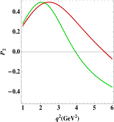
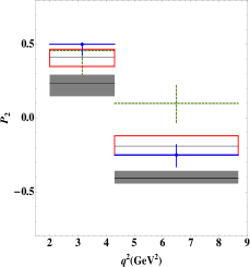
Figure 1: (Left) Exact SM curve for $P_{2}$ (green) and using Eq.(9) (dashed). Exact NP curve for $C_{9}^{NP}=-1.5$ (red) and using Eq.(9) (dashed). (Right) $P_{2}$: Gray band is SM, blue cross is the measured value, red box is $C_{9}^{NP}=-1.5$, green cross dashed is obtained from Eq.(9) using data from $P_{1},P_{4,5}^{\prime}$.

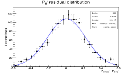
Figure 2: Residual distribution of $P_{5}^{\prime}$ when fitting with 100 events. The fit of a gaussian distribution is superimposed.

The conclusions of this analysis are: i) Eq.(9) in its binned form is a good approximation in most of the bins, except for the bin [0.1-2] GeV² and the bin [1-6] GeV², where the shift becomes sizeable ii) the smaller the bin size the smaller the shift, as expected. The reason why the shift is so large in the first bin is mainly due to the $\beta$ factor that varies strongly in this region. The bin [1-6] GeV² exhibits a large correction given the large size of the bin and the rapid variation of the observables. We have also verified that the upper bound for $P_{1}$ of Eq.(12) is nicely fulfilled in its binned form for all bins given in Table 3 and also in presence of NP. Finally, Eq.(14) can also be used in binned form.

III Implications for data analysis

Under the hypotheses of real Wilson coefficients, we performed a frequentist analysis to test the consistency of LHCb measurements. This was done by generating toy experiments taking as input the measured values of $P_{1}$, $P_{4}^{\prime}$ and $P_{5}^{\prime}$ LHCbpaper , using Eq.(9) to estimate $P_{2}$ and comparing the result of this computation with its measured value in the same bin. The correction of Table 3 for the best fit point ($C_{9}^{NP}=-1.5$) was applied to correct for the binning effect. First of all it should be noted that different $P_{i}$ observables are measured independently, and no constraints that the measurements have to be in the physical region was applied. As a consequence, a fraction of the generated toy experiments are outside the physical region, i.e. where the argument of the square root of Eq. (9) is negative or where Eq. (12) is not satisfied. For the bin [2.0-4.3] GeV² about 50% of the toy experiments fall in the physical region. For the fraction of toy experiments in the physical region, excellent agreement corresponding to 0.2$\sigma$ between the measured value and the value extracted with Eq. (9) is found. For the bin [1.0-6.0] GeV² about 73% of events fall in the physical region. For these events an agreement corresponding to $0.1\sigma$ is observed. Some tensions are found for the third large recoil bin, with $q^{2}$ within [4.3-8.68] GeV² and the first low recoil bin, with $q^{2}$ in the region [14.18-16.00] GeV². In the third large recoil bin only 10% of events satisfy Eq. (12), i.e. the measured value of $P_{1}$ and $P_{4}^{\prime}$ are in tension. For these events a discrepancy of 2.4$\sigma$ between the value of $P_{2}$ computed with Eq. (9) (dashed green cross in Fig.1) and the measured one (solid blue cross in Fig.1) is observed. This discrepancy is not surprising since, as was already pointed out in Ref. thefirst ; conf , the deviation with respect to the value predicted in the SM in the third bin of $P_{5}^{\prime}$ is indeed larger than what the best fit point can explain (notice also that, as discussed in conf , other proposed solutions straub work significantly worse when evaluated in this bin). This is reflected in the fact that the value of $P_{2}$ derived by using Eq. (9) for this bin has a discrepancy of 1.9$\sigma$ from the best fit point, while it has a discrepancy of 3.6$\sigma$ from the SM prediction (see Fig. 1).
The first low recoil bin has about 70% of events within the physical region. For these events a large discrepancy of 3.7$\sigma$ is found between the measured value of $P_{2}$ and the one extracted using ”+” sign in Eq. (9) while agreement is found if ”-” sign is taken. However one would have expected that both signs would give similar results at low recoil.

Under the assumption of real Wilson coefficients it is possible to use Eq. (9) directly in the fit, opening up the possibility to have a full fit of the angular distribution with a small dataset. The free parameters in the fit are the observables $F_{L}$, $P_{1}$, $P_{4}^{\prime}$ and $P_{5}^{\prime}$. The observables $P_{6,8}^{\prime}$ are set to zero, while the observable $P_{2}$ is determined by using Eq.(9). We tested this fit for different values of the observables around the present measured values and we obtained convergence and unbiased pulls with as little as 50 events per bin. This would allow to perform a full fit of the angular distribution with correlations in small bins of $q^{2}$ with relatively small datasets. Gaussians pulls are obtained with as little as 100 events per bin, as shown in Fig. 2 for $P_{5}^{\prime}$. It is worth remarking that the hypothesis of no NP weak phases can be tested by measuring the $P_{i}^{CP}$ observables.

In conclusion, the main question we wanted to address with this paper is if the anomaly in $P_{5}^{\prime}$ measured by LHCb in the third large recoil bin is isolated. We found, using only symmetry arguments, that the anomaly should also appear in $P_{2}$ in a very specific way. By means of the newly presented relation involving $P_{1,2}$, $P_{4,5}^{\prime}$ we have also found that the higher the position of the zero of $A_{FB}$ the smaller the expected value of $P_{5}^{\prime}$ at this point (for a SM-like $P_{4}^{\prime}$), in agreement with LHCb measurements. These results can be used as an independent consistency test of the measurements of the angular observables. A strong constraint on $P_{1}$ shows that, according to Eq.(12), experimental values for $P_{4}^{\prime}\geq 1$ give no space for a large positive $P_{1}$. This rules out those mechanisms coming from right-handed currents that naturally prefer a large positive value for $P_{1}$ in the third large recoil bin, as for instance [$C_{10}^{\prime}<0,C_{9}^{\prime}>0$] or [$C_{10}^{\prime}<0,C_{7eff}^{\prime}>0$]. Finally, by using Eq.(9) directly in the fit to data, under the assumption of no NP weak phases, it is possible to perform a full angular fit with small datasets.

Acknowledgements: J.M. acknowledges support from FPA2011-25948, SGR2009-00894. N.S. acknowledges the support of the Swiss National Science Foundation, PP00P2-144674. We thank Espen Bowen, Olaf Steinkamp and Patrick Koppenburg for reading and commenting this document.

References

- (1) R. Aaij et al. [LHCb Collaboration], JHEP 1308, 131 (2013) [arXiv:1304.6325 [hep-ex]].
- (2) R. Aaij et al. [LHCb Collaboration], Phys. Rev. Lett. 111 (2013) 191801 [arXiv:1308.1707 [hep-ex]].
- (3) F. Kruger and J. Matias, Phys. Rev. D 71, 094009 (2005)
- (4) J. Matias, F. Mescia, M. Ramon and J. Virto, JHEP 1204, 104 (2012) [arXiv:1202.4266 [hep-ph]].
- (5) S. Descotes-Genon, J. Matias and J. Virto, Phys. Rev. D 88 (2013) 074002 [arXiv:1307.5683 [hep-ph]].
- (6) M. Beneke, T. Feldmann and D. Seidel, Nucl. Phys. B 612, 25 (2001) [hep-ph/0106067].
- (7) W. Altmannshofer and D. M. Straub, arXiv:1308.1501
- (8) F. Beaujean, C. Bobeth and D. van Dyk, arXiv:1310.2478
- (9) R. R. Horgan, Z. Liu, S. Meinel and M. Wingate, arXiv:1310.3887 [hep-ph].
- (10) R.Gauld, F.Goertz and U.Haisch, JHEP 1401 (2014) 069
- (11) A. J. Buras, F. De Fazio and J. Girrbach, arXiv:1311.6729 [hep-ph].
- (12) A. Datta, M. Duraisamy and D. Ghosh, arXiv:1310.1937.
- (13) F. Mahmoudi, S. Neshatpour and J. Virto, arXiv:1401.2145 [hep-ph].
- (14) S. Descotes-Genon, T. Hurth, J. Matias and J. Virto, JHEP 1305, 137 (2013) [arXiv:1303.5794 [hep-ph]].
- (15) J. Matias, Phys. Rev. D 86 (2012) 094024 [arXiv:1209.1525 [hep-ph]].
- (16) U. Egede, T. Hurth, J. Matias, M. Ramon and W. Reece, JHEP 1010, 056 (2010) [arXiv:1005.0571 [hep-ph]].
- (17) S. Chatrchyan et al. [CMS Collaboration], Phys. Lett. B 727 (2013) 77
- (18) B. Aubert et al. [BaBar Collaboration], Phys. Rev. D 79 031102 [arXiv:0804.4412 [hep-ex]].
- (19) J. T. Wei et al. [BELLE Collaboration], Phys. Rev. Lett. 103 (2009) 171801 [arXiv:0904.0770 [hep-ex]].
- (20) T. Aaltonen et al. [CDF Collaboration], Phys. Rev. Lett. 108 (2012) 081807 [arXiv:1108.0695 [hep-ex]].
- (21) S. Descotes-Genon, J. Matias and J. Virto, arXiv:1311.3876 [hep-ph].