Chalker scaling, level repulsion, and conformal invariance in critically delocalized quantum matter: Disordered topological superconductors and artificial graphene

Abstract

We numerically investigate critically delocalized wavefunctions in models of 2D Dirac fermions, subject to vector potential disorder. These describe the surface states of 3D topological superconductors, and can also be realized through long-range correlated bond randomness in artificial materials like molecular graphene. A “frozen” regime can occur for strong disorder in these systems, wherein a single wavefunction presents a few localized peaks separated by macroscopic distances. Despite this rarefied spatial structure, we find robust correlations between eigenstates at different energies, at both weak and strong disorder. The associated level statistics are always approximately Wigner-Dyson. The system shows generalized Chalker (quantum critical) scaling, even when individual states are quasilocalized in space. We confirm analytical predictions for the density of states and multifractal spectra. For a single Dirac valley, we establish that finite energy states show universal multifractal spectra consistent with the integer quantum Hall plateau transition. A single Dirac fermion at finite energy can therefore behave as a “Quantum Hall critical metal.” For the case of two valleys and non-abelian disorder, we verify predictions of conformal field theory. Our results for the non-abelian case imply that both delocalization and conformal invariance are topologically-protected for multivalley topological superconductor surface states.

I Introduction

Strong disorder can localize all wavefunctions in a band of energies.Anderson (1958) In a localized phase, states close in energy are peaked at spatially distant centers, implying vanishingly small overlap of the corresponding probability densities. The associated statistics of nearest-neighbor level spacings is Poissonian, i.e. there is no level repulsion. These features imply the similarity of an Anderson insulator to an integrable dynamical system,Huse and Oganesyan an idea ignited by studies of many-body localization.Basko et al. (2006); Oganesyan and Huse (2007); Pal and Huse (2010) By contrast, the states of a diffusive metal are associated with quantum ergodicity, exhibiting Wigner-Dyson level statistics.Sivan and Imry (1987) Near a mobility edge, extended states show quantum critical (Chalker) scalingChalker and Daniell (1988); Chalker (1990) in the overlap of wavefunction probabilities at different energies.Fyodorov and Mirlin (1997); Cuevas and Kravtsov (2007)

In this paper, we examine critically delocalized states in the presence of weak and strong disorder. Such states arise under special circumstances in low dimensions, when protected by symmetries and/or topology.Huckestein (1995); Evers and Mirlin (2008) These states can display non-ergodic characteristics, including a “frozen regime” wherein a single wavefunction can appear almost localized, exhibiting a few isolated peaks separated by macroscopic distances.Chamon et al. (1996); Ryu and Hatsugai (2001a); Carpentier and Le Doussal (2001) In this case, since individual wavefunctions show a mixture of localized and critical features, one might expect a breakdown of correlations between different states with nearby energies. If it were to exist, such a phase could be termed a “non-ergodic” or glassy metal, and would signify a failure of the scaling theory of localization. Possible realizations include the Bethe lattice,Biroli et al. ; Luca et al. the region above the many-body localization transition,de Luca and Scardicchio (2013) or the critical region of the Anderson-Mott metal-insulator transition.Dobrosavljević et al. (2012)

The systems we study consist of 2D massless Dirac fermions coupled to random vector potential disorder. These arise as the surface states of 3D topological superconductors,Schnyder et al. (2008); Foster and Yuzbashyan (2012) in the presence of any surface disorder that respects time-reversal symmetry. (The vector potentials do not encode physical magnetic fields, but instead couple to spin and/or valley currents of gapless surface quasiparticles. These currents are time-reversal even). We consider models in classes AIII and CI, which respectively retain U$(1)$ and SU$(2)$ spin symmetry in every realization of disorder. Class AIII can also be a chiral topological insulator.Hosur et al. (2010)

Specifically, we study a single valley Dirac fermion perturbed by an abelian vector potential,Ludwig et al. (1994) which is the minimal surface state of an AIII topological superconductor.Schnyder et al. (2008) It also arises as the low-energy description of a 2D tight-binding model with long-range correlated random hopping,Motrunich et al. (2002) a system that might be realizable in molecular graphene.Gomes et al. (2012)

We numerically evaluate level spacing statistics, the global density of states (DoS), and multifractal spectraHuckestein (1995); Evers and Mirlin (2008) of single particle wavefunctions. We also compute two-wavefunction correlations between states at different energies. Our work extends previous numericsHatsugai et al. (1997); Morita and Hatsugai (1997); Ryu and Hatsugai (2001b) to stronger disorder (beyond the freezing transition). Prior numerical work on the strong disorder regime investigated the DoSMotrunich et al. (2002) and the multifractal spectrum of the exact zero energy wavefunction.Chen et al. (2012) Our work adds Chalker scaling, level statistics, and multifractal spectra of the low-energy states. Finally, we also investigate a model with two valleys in classes CI and AIII as the simplest example of a Dirac fermion subject to a non-abelian disorder potential.Nersesyan et al. (1994) In our finite size studies, we do not attempt to prove delocalization. Instead, we match our results for the critical behavior of the DoS and multifractal spectra to predictions for the critically delocalized states expected to form in these systems.

Many of the properties of the single-valley model are known analytically. The global DoS is critical. The corresponding dynamical exponent is non-universal and depends on the strength of disorder.Ludwig et al. (1994) The multifractal spectra of the low-energy wavefunctions can be obtained exactly.Ludwig et al. (1994) There is a “freezing transition” driven by the disorder strength in the low-energy states,Chamon et al. (1996); Castillo et al. (1997); Carpentier and Le Doussal (2001) beyond which individual wavefunctions become quasilocalized. The low energy global DoS is also modified in this regime.Motrunich et al. (2002); Horovitz and Doussal (2002); Mudry et al. (2003) Despite this, at the Dirac point the dc (zero temperature, Landauer) conductance is a universal number $e^{2}/\pi h$, valid for arbitrary disorder strength.Ludwig et al. (1994) See Fig. 1 for a comparison of wavefunctions at weak and strong disorder.

Our results imply that energetic correlations survive in this system, even for strong disorder. In particular, after taking into account the critical behavior of the global DoS, we show that the level spacing statistics remain approximately Wigner-Dyson, belowMorita and Hatsugai (1997) and above the freezing transition. Using a long-range correlated random hopping model to simulate the low-energy Dirac fermion physics,Motrunich et al. (2002) we confirm that the overlap between wavefunction probabilities at different energies exhibits a generalized form of Chalker scaling.Chalker and Daniell (1988); Chalker (1990); Huckestein and Schweitzer (1994); Pracz et al. (1996); Fyodorov and Mirlin (1997); Cuevas and Kravtsov (2007); Kravtsov et al. (2010) This also holds below and above freezing, and implies that while individual states become highly rarified in space in the frozen regime, these remain strongly correlated in energy. We conclude that a non-ergodic metal as defined above is not realized here. Strong correlations between nearby eigenstates with rarified structure were also demonstrated in the sparse random matrix model.Fyodorov and Mirlin (1997) We conjecture that “non-ergodic” signatures in energy (Poissonian level statistics, breakdown of Chalker scaling) for single particle states can occur only inside a true Anderson insulator.

We also show that strong disorder has a much weaker and universal effect at larger energies, wherein the multifractal statistics cross over to those of the integer quantum Hall plateau transition, consistent with previous work.Ludwig et al. (1994); Ostrovsky et al. (2007); Nomura et al. (2008) For the non-abelian two-valley model, we confirm predictions of conformal field theory.Nersesyan et al. (1994); Mudry et al. (1996); Caux et al. (1996) Our results for the non-abelian case imply that both delocalization and conformal invariance are topologically-protected for multivalley topological superconductor surface states. At the surface of a topological superconductor in class CI or AIII, gapless quasiparticles are characterized by a well-defined spin conductance (because spin is conserved). Strict conformal invariance is consistent with the universality of the Landauer spin conductance,Ostrovsky et al. (2006) as in the single valley case.Ludwig et al. (1994) The robustness of this result to interaction effects will be explored elsewhere.Xie et al.

The rest of the article is organized as follows: The model of the single valley Dirac fermion and the numerical methods are introduced in Sec. II. We show agreement between the numerical results and the analytical predictions for the global DoS and the zero-energy multifractal spectra in Secs. III and IV, respectively. Level spacing statistics and the correlations between wavefunctions at different energies are studied in Sec. V. The finite energy states of the single-valley model are discussed in Sec. VI. In Sec. VII, we investigate the two-valley model and confirm the conformal field theory predictions. We conclude with a discussion in Sec. VIII.

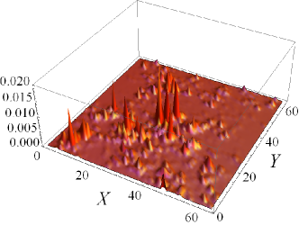
(a) $\Delta_{A}=0.4\pi$, weak disorder region

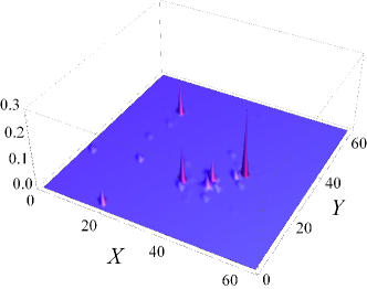
(b) $\Delta_{A}=3\pi$, “frozen” region

Figure 1: Probability density of the exact zero energy wavefunctions in the single valley Dirac fermion model.Ludwig et al. (1994) (a) represents the critically delocalized states in the weak disorder region ($\Delta_{A}<2\pi$). The distribution is spatially inhomogeneous and multifractal. (b) shows the spatial signature of the “frozen” states in the strong disorder region ($\Delta_{A}>2\pi$). The wavefunction is characterized by rarefied peaks. For both cases, we generate the analytical wavefunctionLudwig et al. (1994) with a 64-by-64 spatial resolution.

II Symmetry Properties and Models

Dirac fermions in solid state systems can emerge from graphene(-like) materialsCastro Neto et al. (2009); Das Sarma et al. (2011) and the surfaces of 3D topological matter.Schnyder et al. (2008); Hasan and Kane (2010); Qi and Zhang (2011) In this section, we focus on a single valley Dirac fermion in 2D, subject to a random vector potential. This describes the surface of a 3D time-reversal symmetric topological superconductor with spin U$(1)$ symmetry (class AIII),Schnyder et al. (2008) with surface imperfections due to impurity atoms, vacancies, edge and corner potentials, etc. The Hamiltonian of the 2D Dirac fermion is

$$\mathcal{H} =\int d^{2}\bm{\mathrm{x}}\,\psi^{\dagger}(\bm{\mathrm{x}})\left[-i\bm{\sigma}\cdot\bm{\nabla}+\bm{\sigma}\cdot\bm{\mathrm{A}}(\bm{\mathrm{x}})\right]\psi(\bm{\mathrm{x}})$$ (1)

$$\equiv\int d^{2}\bm{\mathrm{x}}\,\psi^{\dagger}(\bm{\mathrm{x}})\hat{h}(\bm{\mathrm{x}})\psi(\bm{\mathrm{x}})$$

where $\bm{\mathrm{A}}=({A}_{x},{A}_{y})$ is the vector potential and the Dirac pseudospin $\bm{\sigma}=(\sigma_{x},\sigma_{y})$. $\sigma_{x}$ and $\sigma_{y}$ are two of the three standard Pauli matrices.

The Dirac Hamiltonian satisfies a chiral symmetry condition

$$\sigma_{z}\hat{h}\sigma_{z}=-\hat{h}.$$ (2)

Imposing chiral symmetry in every disorder realization implies that the Hamiltonian only allows terms that couple to $\sigma_{x}$ and $\sigma_{y}$.

As mentioned above, Eq. (1) can be viewed as the surface state of a topological superconductor in class AIII. This is a superconductor with a remnant U(1) component of spin SU(2) symmetry, as could arise due to bulk p-wave spin-triplet pairing.Foster and Ludwig (2008); Schnyder et al. (2008) The $z$ component of the physical spin is conserved and plays the role of U(1) charge in this representation. In this intepretation, the pseudospin Pauli matrices $\{\sigma_{\mu}\}$ in Eq. (1) act on a combination of particle-hole and orbital degrees of freedom, but not on the physical spins.Foster et al. Time-reversal and particle-hole symmetries combine to form the chiral condition in Eq. (2). Any disorder terms obeying time reversal symmetry will only appear in the form of vector potential $\bm{\mathrm{A}}$ (up to irrelevant perturbations). Without loss of the generality, one typically considers zero-mean, white-noise-correlated potentials,

$$\langle{A}_{\bar{\alpha}}(\bm{\mathrm{y}})\rangle_{\text{dis}} =0,$$ (3a)

$$\langle{A}_{\bar{\alpha}}(\bm{\mathrm{y}}){A}_{\bar{\alpha}^{\prime}}(\bm{\mathrm{y}}^{\prime})\rangle_{\text{dis}} =\Delta_{A}\,\delta_{\bar{\alpha},\bar{\alpha}^{\prime}}\delta^{(2)}(\bm{\mathrm{y}}-\bm{\mathrm{y}}^{\prime}),$$ (3b)

where $\langle\dots\rangle_{\text{dis}}$ denotes disorder average, and $\Delta_{A}$ determines the disorder strength. In these equations, $\bar{\alpha}$ and $\bar{\alpha}^{\prime}$ span the $x$ and $y$ components.

As discussed in Sec. I, many properties of this model are known analytically. The dc conductance is universal,Ludwig et al. (1994) but various physical quantities like the dynamical critical exponent and the multifractal spectra of the low energy wavefunctions depend on the strength of the disorder $\Delta_{A}$.Ludwig et al. (1994); Chamon et al. (1996); Castillo et al. (1997); Carpentier and Le Doussal (2001)

II.1 Momentum Space Formalism for Dirac fermions

In this section, we describe our numerical momentum space formalism for Dirac fermions (MFD). It is a direct way to simulate the single-valley model in the presence of random potentials.Nomura and MacDonald (2007); Bardarson et al. (2007) The energy cutoff $\Lambda$ is fixed in the MFD simulations. The Fourier transform conventions are given by

$$\widetilde{\psi}_{\bm{\mathrm{n}}} =\frac{1}{\sqrt{L^{2}}}\int d^{2}{\bm{\mathrm{x}}}\,e^{-i\frac{2\pi}{L}\bm{\mathrm{n}}\cdot\bm{\mathrm{x}}}\psi(\bm{\mathrm{x}}),$$

$$\widetilde{{A}}_{\bar{\mu},\bm{\mathrm{n}}} =\int d^{2}{\bm{\mathrm{x}}}\,e^{-i\frac{2\pi}{L}\bm{n}\cdot{\bm{\mathrm{x}}}}{A}_{\bar{\mu}}({\bm{\mathrm{x}}}),$$

where $\bm{\mathrm{n}}=(n_{x},n_{y})$ and $L$ is the length of the system size. We assume periodic boundary conditions so that $n_{x}$ and $n_{y}$ are integer-valued.

The Dirac Hamiltonian in the Fourier space is

$$\mathcal{H}= \,\frac{2\pi}{L}\sum_{\bm{\mathrm{n}}}\widetilde{\psi}^{\dagger}_{\bm{\mathrm{n}}}\left(\bm{\mathrm{n}}\cdot\bm{\mathrm{\sigma}}\right)\widetilde{\psi}_{\bm{\mathrm{n}}}$$

$$\,+\frac{1}{L^{2}}\sum_{\bm{\mathrm{n}},\bm{\mathrm{m}}}\widetilde{\psi}^{\dagger}_{\bm{\mathrm{m}}}\left[\widetilde{A}_{x,\bm{\mathrm{m}}-\bm{\mathrm{n}}}\,\sigma_{x}+\widetilde{A}_{y,\bm{\mathrm{m}}-\bm{\mathrm{n}}}\,\sigma_{y}\right]\widetilde{\psi}_{\bm{\mathrm{n}}}$$

In numerical simulations, we need to introduce two additional scales. These are the cutoff in Fourier modes ($\mathcal{N}$), and the Gaussian correlation length of the disorder potential ($\xi$). The Fourier modes $n_{x}$ and $n_{y}$ are constrained such that $-\mathcal{N}\leq n_{x},\,n_{y}\leq\mathcal{N}$. The momentum grid has size $(2\mathcal{N}+1)^{2}$. The total dimension of the Hilbert space is $2(2\mathcal{N}+1)^{2}$, where the extra factor of 2 accounts for the Dirac pseudospin. We hold constant the energy cutoff $\Lambda=2\pi/r$, where

$$r\equiv L/\mathcal{N}.$$ (4)

$r$ is about twice larger than the finest resolution in the calculations, $L/(2\mathcal{N}+1)$.

On the other hand, the white-noise correlation in Eq. (3b) requires regularization. We replace the delta distribution with a random phase, fixed Gaussian amplitude distribution. We parametrize the disorder potential via

$$\widetilde{{A}}_{\bar{\mu},\bm{\mathrm{n}}}=\sqrt{\Delta_{A}}\,L\exp\left[{\textstyle{-\frac{1}{4}\left(\frac{2\pi}{L}\bm{\mathrm{n}}\xi\right)^{2}}}\right]e^{i\theta_{\bar{\mu},\bm{\mathrm{n}}}}.$$ (5)

where $\theta_{\bar{\mu},\bm{\mathrm{n}}}\in[0,2\pi)$ is a random phase associated with $\widetilde{{A}}_{\bar{\mu},\bm{\mathrm{n}}}$. We take $\theta_{\bar{\mu},\bm{\mathrm{n}}}=-\theta_{\bar{\mu},-\bm{\mathrm{n}}}$ because the $\bm{\mathrm{A}}(\bm{\mathrm{x}})$ is real-valued. The randomness is implemented by assigning a random phase to each Fourier mode. This approach is equivalent to the disorder average up to a finite size correction. We show the validity of the random phase method in the Appendix B. In Eq. (5), the correlation length $\xi$ is of the order of $r$ [Eq. (4)].

In Fig. (2), we sketch the DoS as a function of the energy $E$ in the MFD. High energy states outside the cutoff (red dashed lines) are artifacts of the simulations. There is a region of states (blue circled region) in the vicinity of $E=0$ reflecting the zero-energy quantum critical behavior of the single-valley model. We term this the “chiral region.” The states at intermediate energies above the chiral region and below the cutoff exhibit the linear DoS expected for clean 2D Dirac fermions.

The MFD approach is rather memory intensive because the matrices in momentum space are very dense. The calculations are therefore restricted to small momentum grid sizes.

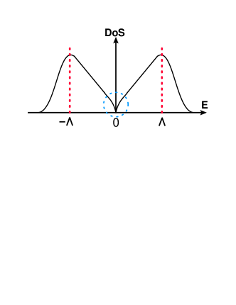
Figure 2: Sketch of the DoS in the MFD, in the presence of disorder. The red dashed lines mark the position of the energy cutoff $\Lambda=\mathcal{N}(2\pi/L)$, which is fixed to a constant. The chiral region is circled by a blue dashed line, wherein the dynamic critical exponent is modified by the disorder strength $\Delta_{A}$.Ludwig et al. (1994); Motrunich et al. (2002); Horovitz and Doussal (2002); Mudry et al. (2003) The states away from the chiral region but inside the cutoff typically show a DoS linear in energy, which is also the result for clean 2D Dirac fermions.

II.2 Lattice Model

As an alternative approach, we study a random hopping model of spinless fermions on a bipartite lattice. The Hamiltonian is

$$\mathcal{H}=\sum_{\langle\bm{\mathrm{r}}_{A},\bm{\mathrm{r}}_{B}\rangle}\left[t_{\bm{\mathrm{r}}_{A},\bm{\mathrm{r}}_{B}}c^{\dagger}_{A}(\bm{\mathrm{r}}_{A})c_{B}(\bm{\mathrm{r}}_{B})+\text{h.c.}\right],$$

where $c^{\dagger}_{A,B}$ ($c_{A,B}$) is the creation (annihilation) operator, $\bm{\mathrm{r}}_{A}$ ($\bm{\mathrm{r}}_{B}$) specifies the position of a point in sublattice $A$ ($B$), and $t_{\bm{\mathrm{r}}_{A},\bm{\mathrm{r}}_{B}}$ is the hopping amplitude between $\bm{\mathrm{r}}_{A}$ and $\bm{\mathrm{r}}_{B}$. The sum runs over nearest-neighbor pairs of sites.

Similar to the Dirac Hamiltonian we wish to study [Eq. (1)], the hopping problem on bipartite lattices defined above satisfies a chiral symmetry (also called sublattice symmetry) at half filling.Gade and Wegner (1991); Gade (1993) Moreover, Dirac fermions can emerge in the low-energy description for specific bipartite lattices (i.e., the honeycomb lattice and the square lattice with $\pi$-flux).Hatsugai et al. (1997); Motrunich et al. (2002)

Unfortunately, sublattice symmetry and low-energy Dirac fermions are insufficient to realize Eq. (1). The latter describes the surface states of a bulk topological superconductor, which one expects cannot be faithfully realized in a microscopic 2D system.Schnyder et al. (2008); Hasan and Kane (2010); Qi and Zhang (2011) For example, the half-filled honeycomb lattice model with bond randomness has an effective description in terms of Dirac fermions with random vector and KekuléHou et al. (2007) mass potentials. The low-energy theory is

$$\mathcal{H}\approx \,v_{F}\int d^{2}{\bm{\mathrm{x}}}\,\psi^{\dagger}\left[-i\sigma_{x}\partial_{x}-i\sigma_{y}\partial_{y}+\bm{\mathrm{A}}\cdot\bm{\mathrm{\sigma}}\kappa_{z}\right]\psi$$ (6)

$$\,+\int d^{2}{\bm{\mathrm{x}}}\,\psi^{\dagger}\left[m_{x}\sigma_{z}\kappa_{x}+m_{y}\sigma_{z}\kappa_{y}\right]\psi,$$

where $v_{F}$ is the Fermi velocity, $\psi$ is the Dirac field [Eq. (40) in the Appendix A], and $\kappa_{z}$ is the valley Pauli matrix. If the system is translationally and rotationally invariant on average, then the mean value of the vector and mass potentials vanish. However, any non-zero variance of the Kekulé mass terms ($m_{x}$ and $m_{y}$) drives the system into the Gade-Wegner fixed point.Gade and Wegner (1991); Gade (1993) This is characterized by a divergent DoS,

$$\nu(E)\sim\frac{1}{E}\exp(-c\left|\ln E\right|^{\alpha}),$$ (7)

where $c$ is a non-universal constant. The exponent $\alpha$ takes the value $1/2$ at intermediate energies,Gade and Wegner (1991); Gade (1993) and crosses over to $2/3$ as $E\rightarrow 0$.Horovitz and Doussal (2002); Motrunich et al. (2002); Mudry et al. (2003) This is different from the Dirac model in Eq. (1), which exhibits a $\Delta_{A}$-dependent power law density of states.

A way to avoid Gade-Wegner physics is to implement the long-range correlated random hopping proposed by Motrunich, Damle, and Huse (MDH) in Ref. Motrunich et al., 2002. The MDH construction is valid for any bipartite lattice with emergent Dirac fermions. One defines a real-valued logarithmic correlated potential $V(\bm{\mathrm{y}})$ via

$$\langle V(\bm{\mathrm{y}})V(\bm{\mathrm{y}}^{\prime})\rangle_{\text{dis}}=-\frac{\Delta_{A}}{2\pi}\ln\left(\frac{|\bm{\mathrm{y}}-\bm{\mathrm{y}}^{\prime}|}{a}\right),$$ (8)

where $a$ is some short distance scale. The hopping amplitudes are generated by

$$t_{\bm{\mathrm{r}}_{A},\bm{\mathrm{r}}_{B}}=t_{\bm{\mathrm{r}}_{B},\bm{\mathrm{r}}_{A}}=e^{V(\bm{\mathrm{r}}_{A})}t_{\bm{\mathrm{r}}_{A},\bm{\mathrm{r}}_{B}}^{\scriptscriptstyle{({0})}}e^{-V(\bm{\mathrm{r}}_{B})},$$ (9)

where $\bm{\mathrm{r}}_{A}$ and $\bm{\mathrm{r}}_{B}$ correspond to nearest-neighbor sites on the A and B sublattices, as depicted in Fig. 3 for both the ($\pi$-flux) square and honeycomb lattices.

The log-correlated disorder is smooth on the lattice scale. Thus, the difference of disorder potentials at nearby positions can be approximated as $V(\bm{\mathrm{y}}+\bm{\mathrm{v}})-V(\bm{\mathrm{y}})\approx(\bm{\mathrm{v}}\cdot\bm{\nabla})V(\bm{\mathrm{y}})$. The low-energy theory can be derived by throwing away second and higher order derivative terms. Mass terms vanish in the naive long wavelength limit. One can show that ${A}_{x}\approx\partial_{y}V$ and ${A}_{y}\approx-\partial_{x}V$ in Eq. (6). The random vector potential $\bm{\mathrm{A}}$ generated this way satisfies Eqs. (3a) and (3b). The low energy theory of the MDH model describes two (nearly) decoupled Dirac fermions with random vector potentials.

It is also important to discuss on the specific coarse graining conditions. On the honeycomb lattice, the Kekulé masses correspond to certain period-3 hopping patterns.Hou et al. (2007) The proper coarse graining cell should be at least as large as a hexagonal plaquette (6 sites, including two sublattices) on the honeycomb lattice. On the contrary, the minimum coarse graining cell on the square lattice with $\pi$-flux is a 2-by-2 block (see Appendix A). We mainly study the MDH model on the square lattice with $\pi$-flux for convenience.

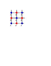
(a) Square lattice with $\pi$-flux

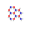
(b) Honeycomb lattice

Figure 3: Bipartite lattices with low-energy Dirac fermions: square lattice with $\pi$-flux and the honeycomb lattice. Labels $A$ and $B$ indicate the sublattices. In the clean limit, the homogeneous hopping amplitudes $t_{\bm{\mathrm{r}}_{A},\bm{\mathrm{r}}_{B}}^{{\scriptscriptstyle{({0})}}}$ [Eq. (9)] are equal to $+1$ for solid lines and $-1$ for dashed lines.

III Dynamical Exponent and Density of States

An important analytical result for the single-valley model is the exact disorder dependenceLudwig et al. (1994); Horovitz and Doussal (2002); Motrunich et al. (2002); Mudry et al. (2003) of the dynamic critical exponent $z$,

$$z=\begin{cases}{}1+\frac{\Delta_{A}}{\pi},&\Delta_{A}\leq 2\pi\\[5.69054pt] 4\sqrt{\frac{\Delta_{A}}{2\pi}}-1,&\Delta_{A}>2\pi\end{cases}$$ (10)

The dynamical exponent shows a non-analyticity at $\Delta_{A}=2\pi$, which signals a “freezing” transitionChamon et al. (1996); Horovitz and Doussal (2002); Motrunich et al. (2002); Mudry et al. (2003) for the low-energy states (discussed in more detail in the next section). The critical behavior of the DoS in the vicinity of zero energy is determined by

$$\nu(E)\propto|E|^{(2-z)/z}.$$ (11)

In our numerical studies, the dynamic critical exponent is extracted from the power-law behavior of the DoS in the chiral region (as shown e.g. in Fig. 2). Instead of calculating the DoS directly, we first defineMotrunich et al. (2002) the quantity $N(E)=\sum_{j}\theta(E_{j})\theta(E-E_{j})$, where $j$ runs over the energy levels and $\theta(x)$ is the Heaviside step function. $N(E)$ is proportional to the DoS integrated over $E$, which has a power law $E^{2/z}$ for $E\rightarrow 0$.

III.1 DoS in MFD Approach

In MFD approach, the white-noise correlation is replaced by a finite-ranged Gaussian distribution. [See Eq. (5) and the discussion following.] The DoS in the chiral region shows power-law behavior for a suitable choice of the Gaussian correlation length $\xi$. In general, the DoS depends on $\Delta_{A}$, $\xi$, and the mode cutoff $\mathcal{N}$. For a given $\Delta_{A}$ and $\mathcal{N}$, we choose a value of $\xi$ such that the power-law exponent reproduces the result in Eq. (10) for the single-valley model. In Fig. 4, we present the power-law behavior of the DoS in this formalism. For $0<\Delta_{A}<\pi$ and $\mathcal{N}=$32, 40, 48, and 64, we are able to obtain the expected power law in Eq. (10) with a fixed common value of the Gaussian correlation length $\xi=0.25r$, where $r=L/\mathcal{N}$ is fixed.footnote–xival

For $\Delta_{A}\geq\pi$, the choice $\xi=0.25r$ can no longer produce the expected power law. Instead of using the fixed value of $\xi$, we explore the $\xi$-dependence of the power law in the DoS. There is an intermediate region where the dependence of the DoS exponent on $\xi$ is rather weak, as exemplified in Fig. 5. We extract the effective dynamical exponent from this insensitive region, and use Eq. (10) to convert this to an effective disorder strength $\Delta_{A,\text{eff}}$. In the sequel, we will use this effective disorder strength to compare analytical and numerical results for level spacing statistics and Chalker scaling. The dynamical exponents extracted for $\Delta_{A}>\pi$ are always smaller than the analytical predictions, so that $\Delta_{A,\text{eff}}<\Delta_{A}$. We assume that the physics in the chiral region is governed by the effective disorder strength $\Delta_{A,\text{eff}}$ rather than the input value of $\Delta_{A}$.

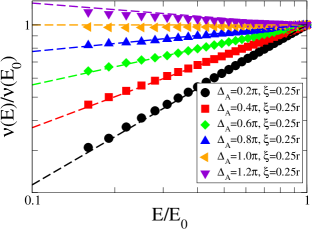
Figure 4: The DoS in MFD near zero energy with $\mathcal{N}=40$, $\xi=0.25r$, and $r=L/\mathcal{N}$. The results were obtained by averaging over 80 realizations of the disorder. Dots are the numerical results from 200 energy levels, and the solid lines are the analytical formula. From bottom to top: $\Delta_{A}=$ $0.2\pi$, $0.4\pi$, $0.6\pi$, $0.8\pi$, $\pi$, and $1.2\pi$. The data are rescaled so that the rightmost points are placed at the same position. As described in the text, for $\Delta_{A}\geq\pi$ we extract an effective disorder strength from the data, which is later employed in the study of level statistics and Chalker scaling. $\Delta_{A,\text{eff}}=0.96\pi$ for $\Delta_{A}=\pi$ and $\Delta_{A,\text{eff}}=1.125\pi$ for $\Delta_{A}=1.2\pi$.

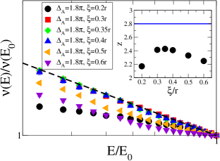
Figure 5: The $\xi$-dependence of the DoS in MFD. $\mathcal{N}=40$, $\Delta_{A}=1.8\pi$, $r=L/\mathcal{N}$, and we average over 20 disorder realizations. Inset: The dynamical exponent $z$ computed with different $\xi$ values. The dots are extracted from the numerical DoS. The blue solid line is the analytical dynamical exponent with $\Delta_{A}=1.8\pi$. We choose $\xi=0.35r$ as the proper parameter in MFD, because this is where $z$ is least sensitive to the value of $\xi$. We extract $\Delta_{A,\text{eff}}\approx 1.42\pi$.

III.2 DoS in MDH Model

The power-law behavior of the DoS in the MDH model has been reported previously.Motrunich et al. (2002) We demonstrate the numerical results for $L=$256 in Fig. 6 for the $\pi$-flux square and honeycomb lattices.

In the weak disorder region $\Delta_{A}<2\pi$, the dynamical exponents fit Eq. (10). In the strong disorder region $\Delta_{A}>2\pi$, the dynamical exponents start to show deviations from the analytical formula. The deviations are due to finite size effects, for instance, finiteness of the mass terms.mas The deviations in the power law are larger in the honeycomb lattice case. This is because the mass terms arise from period-3 Kekulé patterns on the honeycomb lattice, so the corresponding coarse graining cell needs to be at least a 6-site hexagon. For the $\pi$-flux lattice, the smallest coarse graining cell is a 2-by-2 block. For this reason, we expect that the MDH model on the honeycomb lattice will be more sensitive finite size effects than on the $\pi$-flux lattice.

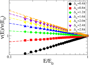
(a) $\pi$-flux lattice

(b) Honeycomb lattice

Figure 6: The DoS near zero energy for the MDH model on (a) the $\pi$-flux lattice with $L=256$ and (b) honeycomb lattice with the same size. Results are averaged over 40 disorder realizations. Dots are the numerical results from 149 energy levels (excluding the first positive level), and the dashed lines are the analytical formula. The data are rescaled such that the rightmost points are placed at the same position.

IV Multifractal Spectra

The zero-energy wavefunction of the single-valley model in the continuum can be written down explicitlyLudwig et al. (1994) for a fixed disordered realization. The exact multifractal spectrumHuckestein (1995); Evers and Mirlin (2008) is known for this state.Ludwig et al. (1994); Castillo et al. (1997); Carpentier and Le Doussal (2001) The multifractal spectrum measures the statistics of the local DoS, which can be measured experimentally by scanning tunneling microscopy.Richardella et al. (2010) It is also a useful tool to understand the characteristics of extended states in disordered environments. One defines the inverse participation ratio (IPR), $P^{(q)}$ via

$$P^{(q)}(b,L)=\sum_{\bm{\mathrm{x}}}|\psi_{b}(\bm{\mathrm{x}})|^{2q}\propto\left(\frac{b}{L}\right)^{\tau(q)},$$ (12)

where $|\psi_{b}(\bm{x})|^{2}$ corresponds to the probability of finding a particle in a box of size $b\ll L$ at position $\bm{\mathrm{x}}$, and $\tau(q)$ is the multifractal exponent associated with the $q$th IPR. $\tau(q)$ is a self-averaging quantityChamon et al. (1996) that satisfies the conditions $\tau(1)=0$ due to the normalization and $\tau(0)=-d$. The latter reflects the dimension of the system, assuming a system volume $L^{d}$. The IPR satisfies the scaling form when $b$ is much larger than any microscopic scale and much smaller than the system size.Huckestein (1995); Evers and Mirlin (2008)

For a fixed system size $L$, the multifractal exponents can be obtained by performing the numerical derivative of $\ln P^{(q)}(b,L)$ with respect to different values of $b$. For example, the $\tau(q)$ for the plane wave is simply $d(q-1)$ because the probability of finding a particle is uniform. In the presence of disorder, critically delocalized wavefunctions extend throughout the sample with an intricate inhomogeneous structure. For weak mulifractality and small $q$, the $\tau(q)$ can be approximated by

$$\tau(q)=d(q-1)-\theta q(q-1),$$ (13)

where $\theta$ can be viewed as the degree of multifractality.

When $q$ exceeds a certain termination thresholdChamon et al. (1996) $q_{\text{c}}$, $\tau(q)$ becomes linearly proportional to $q$. $q_{\text{c}}$ specifies the region violating the parabolic approximation in Eq. (13). The multifractal spectrum for $q>q_{c}$ is governed by an extremum of the probability distribution, and this is represented by a single exponent rather than multiple fractal exponents.

The analytical $\tau(q)$ spectrum for zero energy states shows non-analyticity at $\Delta_{A}=2\pi$. The $\tau(q)$ resultLudwig et al. (1994); Chamon et al. (1996); Castillo et al. (1997); Carpentier and Le Doussal (2001) for $\Delta_{A}\leq 2\pi$ is

$$\tau(q)=\begin{cases}2\left(1-\frac{\Delta_{A}}{2\pi}q\right)(q-1),&0\leq q\leq\sqrt{\frac{2\pi}{\Delta_{A}}},\\ 2\left(1-\sqrt{\frac{\Delta_{A}}{2\pi}}\right)^{2}q,&q>\sqrt{\frac{2\pi}{\Delta_{A}}}.\end{cases}$$ (14)

For $\Delta_{A}\geq 2\pi$,

$$\tau(q)=\begin{cases}-2\left(1-\sqrt{\frac{\Delta_{A}}{2\pi}}q\right)^{2},&0\leq q\leq\sqrt{\frac{2\pi}{\Delta_{A}}},\\ 0,&q>\sqrt{\frac{2\pi}{\Delta_{A}}}.\end{cases}$$ (15)

The termination threshold $q_{c}=\sqrt{\frac{2\pi}{\Delta_{A}}}$ for both regions.

The zero-energy wavefunction shows “freezing” behavior when $\Delta_{A}>2\pi$. The frozen wavefunction is almost zero everywhere, except for several well-localized peaks with arbitrary separations.Chamon et al. (1996); Castillo et al. (1997); Carpentier and Le Doussal (2001) It is qualitatively different from the weakly multifractal extended states with $\Delta_{A}<2\pi$ that fill the sample volume uniformly (but with an intricate structure of many peaks and valleys—see Fig. 1), and from the usual localized state which is dominated by a single peak. The $\tau(q)$ for the frozen state is exactly zero for $q>1\geq q_{c}$, which is the same as a localized state. The multifractal behavior can only be observed for fractional values of $q$.

A related quantity is the singularity spectrumEvers and Mirlin (2008) $f(\alpha)$, defined by the Legendre transformation of $\tau(q)$

$$f(\alpha)=\alpha q-\tau(q),$$ (16)

where $\alpha=d\tau/dq$. The physical interpretation of $f(\alpha)$ is the following. Assume there is a collection of points in position space where the probability density $|\psi(\bm{\mathrm{x}})|^{2}\propto L^{-\alpha}$. Then the number of such points scales as $L^{f(\alpha)}$. For example, for a plane wave the $f(\alpha)$ spectrum is zero everywhere except $\alpha=d$. For a multifractal wavefunction, $f(\alpha)$ is a peaked function with non-zero width. The spectrum gets broader with increasing multifractality.

There are a handful of general properties regarding $f(\alpha)$. When $\alpha=\alpha_{0}\equiv(d\tau/dq)|_{q=0}$, $f(\alpha_{0})=d$ is maximized. When $\alpha=\alpha_{1}\equiv(d\tau/dq)|_{q=1}$, $f(\alpha_{1})=\alpha_{1}$ and $f^{\prime}(\alpha_{1})=1$.

The analytical $f(\alpha)$ for the zero-energy wavefunction is given byChamon et al. (1996); Castillo et al. (1997)

$$f(\alpha)=8\frac{(d_{+}-\alpha)(\alpha-d_{-})}{(d_{+}-d_{-})^{2}}.$$ (17)

In the weak disorder regime $0\leq\Delta_{A}<2\pi$,

$$d_{\pm}=2\left({\textstyle{1\pm\sqrt{\frac{\Delta_{A}}{2\pi}}}}\right)^{2}.$$ (18)

In the frozen phase $\Delta_{A}\geq 2\pi$,

$$d_{-} =0,\,\,\,d_{+}=8\sqrt{\frac{\Delta_{A}}{2\pi}}.$$ (19)

$d_{-}=0$ indicates that $f(0)=0$. This is the signature of freezing in the $f(\alpha)$ spectrum.

In our simulations, we select the first positive energy state as representative. It is important to note that all the wavefunctions in the chiral region show similar multifractal characteristics reflecting the (effective) disorder strength dependence in the low-energy theory for both the MFD and MDH models.

IV.1 Multifractal Spectra in MFD

We first consider the results of our momentum space Dirac (MFD) calculations. The multifractal spectra are consistent with Eqs. (17) and (18) for $\Delta_{A}\leq\pi$. These results are shown in Fig. 7. For $\Delta_{A}=\pi$, the multifractal spectrum in MFD shows deviations from the analytical formulas. It is difficult to extract strong multifractal phenomena such as freezing using the MFD approach, due to finite size limitations. The finest spatial resolution in MFD is determined by the $(2\mathcal{N}+1)$-by-$(2\mathcal{N}+1)$ grid. However, it contains some short-distance artifacts due to the high momentum states ($|\bm{\mathrm{k}}|>\Lambda$) [see Fig. 2]. Instead, we convert our wavefunction in MFD to an $\mathcal{N}$-by-$\mathcal{N}$ grid. Our grid sizes for MFD are 32-by-32, 40-by-40, 48-by-48, and 64-by-64. Calculating the IPR in this formalism is restricted by $\mathcal{N}$ and the value of $\xi$. The wavefunctions with such small grid sizes can only represent weak multifractality.

We find that states with energy sufficiently away from the chiral region show universal weak multifractality, consistent with the critical states of the integer quantum Hall plateau transition. We postpone the discussion to Sec. VI.

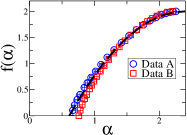
(a) $\Delta_{A}=0.4\pi$, $\xi=0.25r$

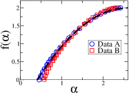
(b) $\Delta_{A}=0.6\pi$, $\xi=0.25r$

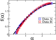
(c) $\Delta_{A}=0.8\pi$, $\xi=0.25r$

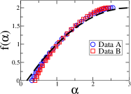
(d) $\Delta_{A}=1.0\pi$, $\xi=0.25r$

Figure 7: The $f(\alpha)$ spectra of low energy states in MFD with $\mathcal{N}=40$. For each value of $\Delta_{A}$, results are averaged over 40 disorder realizations. Here $r=L/\mathcal{N}$. The data are extracted from the numerical derivative of the IPR with respect to $b$, the size of the binning cell. Data A is extracted from $b=1$ and $b=2$. Data B is extracted from $b=2$ and $b=4$. The solid lines are the analytical prediction from Eqs. (17) and (18).

IV.2 Multifractal Spectra in the MDH Model

In order to simulate Dirac fermions coupled only to vector potential disorder with the MDH model, one has to perform a coarse graining (binning) procedure. For the square lattice with $\pi$-flux, the binning size $b$ needs to be at least twice larger than the lattice constant (corresponding to a 2-by-2 coarse graining cell). We calculate the multifractal spectrum for $L=$128, 256, and 512. The finite size scaling of the single-valley model contains $1/\ln L$ and $\ln\ln L/\ln L$ terms.Carpentier and Le Doussal (2001) In this aspect, it is difficult to obtain reliable finite size scaling. The $f(\alpha)$ spectra for different sizes are almost identical in our simulations. We only present multifractal spectra with $L=256$ in the Fig. 8. The results fit the analytical formula for $f(\alpha)$ in Eq. (17), and in particular reveal the signature $f(0)=0$ for the frozen regime with $\Delta_{A}=2\pi$ and $2.4\pi$.

The finite energy states of the MDH model are expected to be localized in the thermodynamic limit.Motrunich et al. (2002) Only the states in the chiral region reflect the physics of the Dirac fermion with the random vector potential.

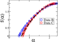
(a) $\Delta_{A}=0.4\pi$

(b) $\Delta_{A}=0.8\pi$

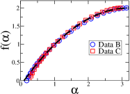
(c) $\Delta_{A}=1.2\pi$

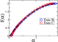
(d) $\Delta_{A}=1.6\pi$

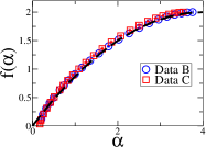
(e) $\Delta_{A}=2.0\pi$

(f) $\Delta_{A}=2.4\pi$

Figure 8: The $f(\alpha)$ spectra of low energy states of the MDH model with $L=256$. For each value of $\Delta_{A}$, results are averaged over 40 disorder realizations. The data are extracted from the numerical derivative of the IPR with respect to $b$, the size of the binning cell. Data B is extracted from $b=2$ and $b=4$. Data C is extracted from $b=4$ and $b=8$. The solid lines are the analytical prediction from Eqs. (17), (18), and (19).

V Level statistics and Chalker scaling in the single valley model

The exact zero energy wavefunction in the single-valley model has been extensively studied.Ludwig et al. (1994); Chamon et al. (1996); Castillo et al. (1997); Hatsugai et al. (1997); Carpentier and Le Doussal (2001); Chen et al. (2012) Besides the global density of states,Morita and Hatsugai (1997); Motrunich et al. (2002); Horovitz and Doussal (2002); Mudry et al. (2003) the properties of low-energy states have received less attention. We focus on two quantities related to correlations between states at different energies: the level spacing distribution and the two-wavefunction correlation. The former measures the distribution of gaps between nearby levels. It is also a useful probe for Anderson localization. On the other hand, the two-wavefunction correlation function characterizes the overlap of the probability distributions for two wavefunctions at different energies. In this section, we numerically study the level spacing distribution and the two-wavefunction correlation in the MFD and MDH models. We show that states at different energies are strongly correlated in the chiral region, for both weak and strong disorder. Our main conclusion is that the spectral characteristics discussed here do not exhibit clear signatures of the freezing transition observed in multifractal spectra and in the density of states.

V.1 Level Spacing Distribution

In a random quantum system, one can view the exact level spectrum in a fixed realization of the disorder as arising through the perturbative sewing together of spatially segregated subsystems. In a metallic phase, nearby energy levels repel each other.Sivan and Imry (1987) States avoid level crossings due to the finite overlap of their spatial distributions. By contrast, in an Anderson insulator, different states can be arbitrarily close in energy because the spatial overlap of their probability densities is essentially zero. The distribution of energy levels therefore reflects the localization properties of the phase.Mirlin (2000)

In the single-valley Dirac model, a representative wavefunction in the frozen regimeChamon et al. (1996) that occurs for strong disorder $(\Delta_{A}>2\pi)$ typically possesses rare peaks with arbitrarily large separation between them.Ryu and Hatsugai (2001a); Carpentier and Le Doussal (2001) These states appear “quasi-localized,” as indicated by the vanishing multifractal spectrum $\tau(q)$ for $q>1$ [Eq. (15)]; see also Fig. 1. We might expect that the level spacing distribution will reflect this, i.e. show Poissonian, rather than Wigner-Dyson statistics. On the other hand, states at weak disorder are weakly multifractal and extended. In fact, our results show no signature of the freezing transition in the level spacing distribution. In both the MFD and MDH models, the distributions are essentially independent of the disorder strength, and are well-approximated by the Wigner surmise in the host model at non-zero energies.

We first define the level spacing distribution function $P(s)$, which satisfies

$$\int_{0}^{\infty}P(s)ds=1,\;\;\int_{0}^{\infty}sP(s)ds=1,$$ (20)

where $s=|E_{n}-E_{n+1}|/\delta(E_{n})$ is the normalized level spacing. Here $\delta(E_{n})$ is the mean level spacing near energy $E_{n}$. Diffusive metals in the Wigner-Dyson symmetry classesMirlin (2000) can be described by the Wigner surmise $P(s)=As^{\beta}\exp(-Bs^{2})$, where $A$ and $B$ are determined by Eq. (20). The parameter $\beta=\{1,2,4\}$ in the orthogonal, unitary, and symplectic classes, respectively. For localized states, the distribution is Poissonian $P(s)=e^{-s}$.

In the single-valley Dirac problem, the DoS $\nu(E)$ changes rapidly in the low-energy chiral region; see Eqs. (10) and (11), and Figs. 2, 4, and 6. For both of the numerical MFD and MDH approaches, we define the level distribution function by rescaling energy level intervals relative to the local mean spacing $\delta(E)\propto 1/\nu(E)$.Evangelou and Katsanos (2003)

In the MFD approach, we find that $P(s)$ in the chiral region fits the Wigner surmise with $\beta=2$ (unitary metal) for all the disorder strengths we explored, $0.4\pi\leq\Delta_{A,\text{eff}}\leq 2.55\pi$ (see Fig. 9). The distributions are independent of $\Delta_{A,\text{eff}}$. (The procedure used to define the effective disorder strength $\Delta_{A,\text{eff}}$ was explained in Sec. III.1.)

In the MDH model, $P(s)$ also exhibits level repulsion, as shown in Fig. 10. We exclude the first energy interval because the first two levels are degenerate when $L\rightarrow\infty$. The results are close to the Wigner surmise with $\beta=1$ (orthogonal metal) rather than $\beta=2$. There are deviations from the Wigner surmise (particularly in the tail), consistent with a previous report.Morita and Hatsugai (1997) In the limit $L\rightarrow\infty$, the finite-energy states in the MDH model are always localized. The levels we sampled are in the chiral low-energy region, and reveal the same critical properties (dynamic critical exponent, multifractal spectra) as the single-valley Dirac model. For states in the MDH model sufficiently away from the chiral region, the level spacing distribution is Poissonian, which indicates localization.

The results for the MFD and MDH models suggest that the level statistics in the chiral region are independent of the disorder strength. At finite energy, the character of the (de)localization problem in these models is the same as that obtained by adding a non-zero chemical potential to the single particle Hamiltonian. This breaks the special chiral symmetry [Eq. (2)], reducing the system to one of the standard Wigner-Dyson classes. The single Dirac fermion model crosses over to the unitary class at finite energy (MFD approach), while the MDH lattice model crosses over to the orthogonal class. Evidently the level statistics for these states reflect only the symmetry class of the “host” model at finite energy. In particular, $P(s)$ shows no signs of the freezing transition in the MDH model, despite the fact that we do observe signatures in the DoS and multifractal spectrum (Figs. 6 and 8). The results imply that the overlap of probabiltiy densities associated with different wavefunctions is non-negligible, even for states in the frozen regime.

Figure 9: The level spacing distribution in the chiral region of the Dirac fermion in MFD. Here the system size is $\mathcal{N}=32$, we keep 100 energy levels per realization, and we have averaged over 400 disorder realizations; $r=L/\mathcal{N}$. The effective disorder strength $\Delta_{A,\text{eff}}$ for the presented data is $0.4\pi$, $1.55\pi$, $1.9\pi$, and $2.55\pi$. Inset: The tail distribution. The black solid line is the Wigner surmise with $\beta=2$; the blue solid line is the Poisson distribution.

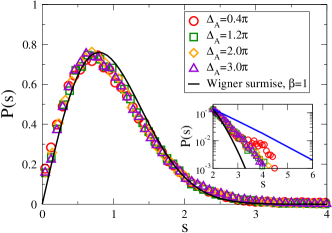
Figure 10: The level spacing distribution in the chiral region of the MDH model. The system size is $L=256$, we keep 149 energy levels per realization, and we have averaged over 400 disorder realizations. Inset: The tail distribution. The black solid line is the Wigner surmise with $\beta=1$; the blue solid line is the Poisson distribution.

V.2 Two-Eigenfunction Correlation

To further characterize effects of weak and strong disorder, we compute the correlations between two wavefunctions at different energies in the same disorder realization.Chalker and Daniell (1988); Chalker (1990); Huckestein and Schweitzer (1994); Pracz et al. (1996); Fyodorov and Mirlin (1997); Cuevas and Kravtsov (2007); Kravtsov et al. (2010) The correlation function in $d$ spatial dimensions is defined by

$$C(E_{0},E_{0}+\epsilon;L)=\int d^{d}{\bm{\mathrm{x}}}\,|\psi_{0}(\bm{\mathrm{x}})|^{2}|\psi_{\epsilon}(\bm{\mathrm{x}})|^{2},$$ (21)

where $E_{0}$, $E_{0}+\epsilon$ are eigenenergies of the system, and $\psi_{0}$, $\psi_{\epsilon}$ are the corresponding wavefunctions. $C(E_{0},E_{0}+\epsilon;L)$ reduces to the inverse participation ratio (IPR) [Eq. (12)] with $q=2$ when $\epsilon=0$.

This correlation function shows different behavior when evaluated in a region of extended or localized states. In particular, $C(E_{0},E_{0}+\epsilon;L)\sim 0$ for localized states with $0<\epsilon\ll\delta_{l}$, where $\delta_{l}$ is the level spacing in a characteristic localization volume. This result obtains because states with nearby energies are typically separated in real space, so that the probability densities of the two wavefunctions have negligble overlap for all $\bm{\mathrm{x}}$. On the other hand, for states near a mobility edge, $C(E_{0},E_{0}+\epsilon;L)$ shows non-trivial scalingChalker and Daniell (1988); Chalker (1990); Fyodorov and Mirlin (1997); Cuevas and Kravtsov (2007) in $\epsilon$. To simplify notation, we suppress the argument $E_{0}$ in the later discussion, $C(E_{0},E_{0}+\epsilon;L)\equiv C(\epsilon;L)$.

In order to understand the scaling behavior of $C$, we define

$$F(\epsilon;L)\equiv\frac{\int d^{d}{\bm{\mathrm{x}}}\,|\psi_{0}(\bm{\mathrm{x}})|^{2}|\psi_{\epsilon}(\bm{\mathrm{x}})|^{2}}{\int d^{d}{\bm{\mathrm{x}}}\,|\psi_{0}(\bm{\mathrm{x}})|^{4}}.$$ (22)

The general scaling form is

$$F(\epsilon;L)=\left(\frac{a}{L}\right)^{\delta}f(\epsilon L^{z}),$$ (23)

where $\delta$ is some scaling exponent and $a$ represents a short distance scale. The exponent $\delta$ must be zero because $F(0;L)$ is normalized to unity. We assume that $f(x)\sim x^{-\mu}$ for large $x$, which implies that

$$\lim_{L\rightarrow\infty}C(\epsilon;L)\sim\frac{\epsilon^{-\mu}}{L^{d_{2}+\mu z}},$$ (24)

where $d_{2}=\tau(2)$ is the correlation dimension. On the other hand, the scaling behavior for large $\epsilon$ should be determined by integration over the product of the two eigenstate probability densities, instead of the second IPR. This implies that

$$\mu=\frac{d-d_{2}}{z},$$ (25)

where $d$ is the spatial dimension. The result in Eq. (25) generalizes the well-known Chalker scaling exponentChalker and Daniell (1988); Chalker (1990) to a system with a critical low-energy DoS ($z\neq d$).

When $E_{0}=0$ in Eq. (21), the disorder dependent formula for $\mu$ is

$$\mu=\begin{cases}\frac{2\Delta_{A}/\pi}{1+\Delta_{A}/\pi},&0\leq\Delta_{A}\leq\frac{\pi}{2},\\[5.69054pt] \frac{2-4\left(1-\sqrt{\Delta_{A}/(2\pi)}\right)^{2}}{1+\Delta_{A}/\pi},&\frac{\pi}{2}<\Delta_{A}\leq 2\pi,\\[5.69054pt] \frac{2}{4\sqrt{\Delta_{A}/(2\pi)}-1},&2\pi<\Delta_{A}.\end{cases}$$ (26)

There are three regimes of the exponent $\mu$. The multifractal dimension $d_{2}=\tau(2)$ has two non-analyticities at $\Delta_{A}=\pi/2$ and $\Delta_{A}=2\pi$; the dynamical exponent $z$ has a transition at $\Delta_{A}=2\pi$. For $\Delta_{A}<\pi/2$, $\mu$ is monotonically increasing and can be determined by the first expression in each of Eqs. (10) and (14). When $\Delta_{A}$ is larger than $\pi/2$ ($q_{c}=\sqrt{2\pi/\Delta_{a}}<2$), one needs to apply the formula for termination in Eq. (14). In the frozen regime $\Delta_{A}>2\pi$, $d_{2}=0$ and the dynamical exponent is given by the second result in Eq. (10).

We calculate the disorder-averaged $C(\epsilon;L)$ for $E_{0}=0$ in the chiral region for both the MFD and MDH models. The numerical exponent shown in Fig. 11 is qualitatively consistent with generalized Chalker scaling [Eq. (26)] for weak disorder in MFD and for disorder strengths up to and beyond the freezing transition ($\Delta_{A}\leq 3\pi$) in the MDH model. For the MFD calculations, we plot $\mu$ versus the effective disorder strength $\Delta_{A,\text{eff}}$ for $\Delta_{A}>\pi$, as defined in Sec. III.1. The good agreement of the MDH model numerics with the analytical prediction indicates the presence of strong correlations between the probability density profiles (peaks and valleys) of different eigenstates, for both weak and strong disorder. We conclude that while individual wavefunctions are strongly inhomogeneous in space in the frozen regime, quantum critical scaling survives—the spectral characteristics remain “ergodic.”

The discrepancy in the MFD result for the generalized Chalker scaling exponent $\mu$ might come from finite system size limitations to this approach. Similar to the situation for multifractal spectra, a high resolution is essential to extract the correct correlations from the critical wavefunctions. For the MDH model, we perform the coarse graining procedure described in Sec. IV.2 to the wavefunctions with binning size $b=2$.

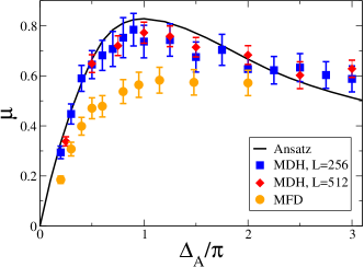
Figure 11: The Chalker scaling exponent $\mu$ [defined via Eq. (24)] as a function of the disorder strength in the MFD and MDH approaches. $\mathcal{N}=40$ and we average over 80 realizations of the disorder for MFD. We show data for two system sizes of the MDH model. For $L=256$, we average over 200 realizations of the disorder. For $L=512$, we average over 40 disorder realizations. For MFD, the effective disorder strengths are presented when $\Delta_{A}>\pi$. For the MDH model, the wavefunctions are coarse-grained with binning size $b=2$. The solid curve is the analytical prediction that includes termination and freezing effects, Eq. (26).

VI Quantum Hall Critical Metal: Finite Energy States

In this section, we discuss the finite energy states of the single-valley Dirac model. These belong to the unitary class (class A).Ludwig et al. (1994) In two dimensions, this class is always localized except in the presence of topological protection. The finite energy physics of the single-valley model with vector potential disorder is expected to be the same as that of the low-energy states for a single Dirac fermion subject to any combination of zero-mean mass, scalar, or vector disorder potentialsLudwig et al. (1994) (i.e., at least two types with non-zero variance). The states are expected to be critically delocalized at all energies, with critical properties governed by the plateau transition of the integer quantum Hall effect.Ludwig et al. (1994); Nomura et al. (2008); Ostrovsky et al. (2007)

We sample states around energy $\sim 0.6\Lambda$ with $\mathcal{N}=$32, 40, 48, and 64 in MFD, where $\Lambda=\mathcal{N}(2\pi/L)$ is the energy cutoff. The level spacing distribution is consistent with the Wigner surmise for the unitary metal, independent of the disorder strength. (Results are quantitatively the same as in Fig. 9). In addition, the multifractal spectra show rather universal behavior. These are presented for various disorder strengths in Fig. 12. The singularity spectrum $f(\alpha)$ shows saturation for $\Delta_{A}\geq 0.8\pi$. The saturated spectrum is close to

$$f(\alpha)=2-\frac{1}{4\theta}(\alpha-2-\theta)^{2},$$ (27)

with $\theta\approx 0.26$. This is the Legendre transform of the pure parabolic $\tau(q)$ spectrum in Eq. (13), which describes to a good approximation the multifractal spectrum for the integer quantum Hall plateau transition.Evers et al. (2001, 2008); Obuse et al. (2008)

Our result is the first numerical evidence for the delocalization of the finite energy states in the single-valley model based on the universal multifractal spectrum for the integer quantum Hall plateau transition. For comparison, we also show $f(\alpha)$ for a single-valley Dirac fermion in the presence of two different types of disorder in Fig. 13.

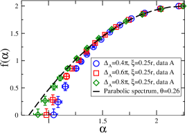
(a) Weak disorder

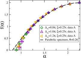
(b) Intermediate disorder

Figure 12: The $f(\alpha)$ spectra of finite energy states in the single-valley Dirac model using the momentum space formalism with $\mathcal{N}=40$. We perform an average over 80 realizations of the disorder; $r=L/\mathcal{N}$. Finite energy states with $\Delta_{A}=0.4\pi$ and $\Delta_{A}=0.6\pi$ show deviations from the parabolic spectrum in Eq. (27) with $\theta=0.26$. The latter is a good approximation to the integer quantum Hall plateau transition spectrum.Evers et al. (2001, 2008); Obuse et al. (2008) For $\Delta_{A}=0.8\pi$, $\pi$, and $1.2\pi$, the $f(\alpha)$ spectra are consistent with the $\theta=0.26$ curve. $\Delta_{A,\text{eff}}=0.96\pi$ for $\Delta_{A}=\pi$, and $\Delta_{A,\text{eff}}=1.125\pi$ for $\Delta_{A}=1.2\pi$. Data A is extracted from $b=1$ and $b=2$.

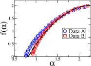
(a) $\Delta_{A}=\Delta_{M}=0.8\pi$

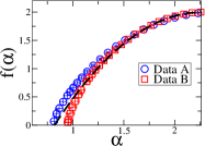
(b) $\Delta_{V}=\Delta_{A}=0.8\pi$

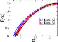
(c) $\Delta_{V}=\Delta_{M}=0.8\pi$

Figure 13: The $f(\alpha)$ spectra of low energy states for a single-valley Dirac fermion with two kinds of disorder in MFD; $\mathcal{N}=40$. We perform an average over 80 realizations of the disorder. $\Delta_{V}$ and $\Delta_{M}$ correspond to the disorder variance of scalar and mass potentials, respectively. $\xi=0.25r$ for all the cases, where $r=L/\mathcal{N}$. Data A is extracted from binning sizes $b=1$ and $b=2$. Data B is extracted from $b=2$ and $b=4$. The dashed line is the same as stated in Fig. 12.

VII Non-Abelian Vector Potential Dirac Fermions

Bulk topological superconductors in classes CI and AIII can host multiple surface Dirac bands. The number of species (or: “valleys”) of Dirac fermions at the surface is equal to the modulus of the corresponding bulk winding number $|\nu|$.Schnyder et al. (2008) For a superconductor with $|\nu|>1$, spin SU(2) and time-reversal invariant disorder manifests as a non-abelian valley vector potential in the low-energy surface Dirac theory, which can mediate both intra- and intervalley scattering. This encodes the effects of charged impurities, vacancies, as well as corner and edge potentials on the surface.Foster et al.

We focus on the two-valley model as the simplest example of Dirac fermions subject to non-abelian vector potentials. The two-valley Dirac Hamiltonian is

$$\mathcal{H} =\int d^{2}\bm{\mathrm{x}}\,\psi^{\dagger}(\bm{\mathrm{x}})\left[-i\bm{\sigma}\cdot\bm{\nabla}+\bm{\sigma}\cdot\bm{\mathrm{A}}_{0}(\bm{\mathrm{x}})\right]\psi(\bm{\mathrm{x}})$$ (28)

$$+\int d^{2}\bm{\mathrm{x}}\,\psi^{\dagger}(\bm{\mathrm{x}})\left[\sum_{a=x,y,z}\kappa_{a}\bm{\sigma}\cdot\bm{\mathrm{A}}_{a}(\bm{\mathrm{x}})\right]\psi(\bm{\mathrm{x}}),$$ (29)

where $\bm{\mathrm{A}}_{a}$ couples to the valley space Pauli matrix $\kappa_{a}$ ($a\in\{x,y,z\}$), and $\bm{\mathrm{A}}_{0}$ is an abelian vector potential, as appears in the single valley case. We implement the random abelian and non-abelian vector potentials in the momentum space Dirac fermion (MFD) scheme described in Sec. II.1. The disorder variance for the non-abelian potential is denoted by $\Delta_{N}$. In the absence of the abelian vector potential, the system belongs to class CI,Schnyder et al. (2008, 2009); Foster and Yuzbashyan (2012) and can be realized at the surface of a spin SU(2) invariant topological superconductor. A non-zero abelian potential couples to the U(1) spin current, associated with the conserved component of spin. [This is the U(1) charge of the Dirac quasiparticle field $\psi$, which carries well-defined angular momentum but not electric charge.Foster et al. ] When both the abelian and non-abelian vector potentials are present, the model resides in class AIII as in the single valley case. A topological superconductor in class AIII can be realized if time-reversal and a remnant U(1) of the spin SU(2) symmetry is preserved in every realization of the disorder, as might arise, e.g., through spin-triplet p-wave pairing.Foster and Ludwig (2008); Schnyder et al. (2008)

The problem of 2D Dirac fermions coupled to random vector potentials is exactly solvable by methods of conformal field theory;Nersesyan et al. (1994, 1995); Mudry et al. (1996); Caux et al. (1996); Foster and Yuzbashyan (2012) for a review, see e.g. Ref. Foster et al., . The relevant theory for a topological superconductor surface state with winding number $|\nu|$ is a Wess-Zumino-Witten model at level $|\nu|/2$ ($|\nu|$) in class CI (AIII).Schnyder et al. (2009); Foster and Yuzbashyan (2012); Foster et al.

For the system at the Wess-Zumino-Witten fixed point, the critical behavior of the global DoSNersesyan et al. (1994, 1995); Foster and Yuzbashyan (2012) and the multifractal spectrumMudry et al. (1996); Caux et al. (1996) of local density of states fluctuations can be calculated exactly. For the two-valley case, the dynamic critical exponent is given by

$$z=\frac{7}{4}+\frac{\Delta_{A}}{\pi}.$$ (30)

This result is independent of the non-abelian disorder strength, and becomes universal when $\Delta_{A}\rightarrow 0$. As in the abelian model, a freezing transition is expected to take place when $\Delta_{A}$ is larger than a certain threshold value (equal to $7\pi/4$ for two valleys). The multifractal spectrum is exactly parabolic, up to termination. For two valleys, the parameter $\theta$ in Eqs. (13) and (27) takes the valueMudry et al. (1996); Caux et al. (1996)

$$\theta=\frac{1}{4}+\frac{\Delta_{A}}{\pi}.$$ (31)

We use MFD to compute $z$ and the multifractal spectrum for two-valley surface states, using grid sizes $\mathcal{N}=32$ to $48$. In Fig. 14, the critical behavior of the DoS [related to $z$ via Eq. (11)] found numerically agrees well with the analytical prediction implied by Eq. (30). Moreover, the $f(\alpha)$ spectra shown in Fig. 15 are also close to the analytical predictions.

The numerical data shows good agreement with the conformal field theory results. This appears to imply that the topology protects both the delocalization of the wavefunctions and the strict conformal invariance of the surface. To understand this, we consider a perturbation of the class CI and AIII Wess-Zumino-Witten models. In the conformal limit, the coefficient $1/\lambda$ of the gradient term in the non-abelian bosonization of these theories is equal to the level $k$.Di Francesco et al. (1996); Foster et al. If we deform $\lambda$ away from this, we get a non-conformal theory (principle chiral model with a Wess-Zumino-Witten term). In the large-$k$ limit, the lowest order RG equations are given byWitten (1984); Guruswamy et al. (2000); Foster et al.

CI: $$\frac{d\lambda}{dl}=\lambda^{2}\left[1-(k\lambda)^{2}\right],$$ (32a)

AIII: $$\frac{d\lambda}{dl}=0,\,\,\frac{d\Delta_{A}}{dl}=\pi\lambda^{2}\left[1-(k\lambda)^{2}\right].$$ (32b)

In class CI, the deformation is irrelevant: Eq. (32a) implies that the system flows back to the conformal limit ($\lambda=1/k$). On the other hand, in class AIII Eq. (32b) implies that the abelian disorder variance $\Delta_{A}$ becomes scale dependent whenever $\lambda\neq 1/k$. Although Eq. (32b) can be obtained by perturbation theory in $\lambda\sim 1/k$, valid in the limit $k\gg 1$, these results turn out to be exact.Guruswamy et al. (2000) We conclude that any deformation away from the conformal limit in class AIII induces a runaway flow of $\Delta_{A}$. As a result, one finds Gade-Wegner physics,Gade and Wegner (1991); Gade (1993) wherein the DoS assumes the strongly divergent form in Eq. (7). The low-energy wavefunctions should always exhibit frozen multifractal spectra.

Although we are limited to small system sizes, we do not observe any signatures of the Gade-Wegner scaling in class AIII. For example, the low-energy DoS vanishes for $0<\Delta_{A}<\pi/4$, as indicated in Fig. 14. Moreover, the multifractal spectra in Fig. 15 are consistent with the parabolic spectra implied by Eq. (31). These suggest that the disordered Dirac theory in Eq. (28) flows under the renormalization group directly to the AIII conformal field theory, without inducing the perturbation $\lambda\neq 1/k$. As discussed in Refs. Foster et al., ; Xie et al., , this is consistent with the resultLudwig et al. (1994); Tsvelik (1995); Ostrovsky et al. (2006) that the Landauer (spin) conductance is universal for non-interacting 2D Dirac fermions coupled to random vector potentials. It is then natural to interpret the coupling strength $\lambda=1/k$ of the Wess-Zumino-Witten theory as the inverse Landauer spin conductance. As discussed elsewhere,Xie et al. ; Foster et al. the lowest-order interaction corrections to the conductance also vanish. These results suggest the possibility that the surface state spin conductance of a topological superconductor is truly universal (i.e., independent of both disorder and interactions), and provides a way to measure the bulk winding number directly via transport, without modifying the surfaceHasan and Kane (2010); Qi and Zhang (2011) in some special way.

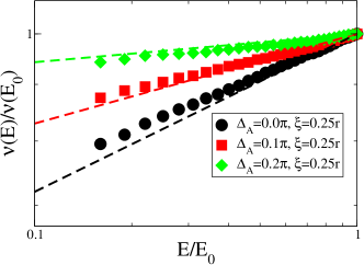
Figure 14: The DoS near zero energy for 2-valley class CI and AIII Dirac models, with $\mathcal{N}=40$. Dots are the numerical results from 400 energy levels, averaged over 40 disorder realizations. The strength of the non-abelian SU(2) vector potential disorder $\Delta_{N}$ is fixed to $0.8\pi$ for all three cases; $r=L/\mathcal{N}$. The case(s) with $\Delta_{A}=0$ ($\Delta_{A}>0$) correspond to class CI (AIII). The solid lines are the analytical result implied by Eqs. (11) and (30). The data are rescaled so that the rightmost points are placed at the same position.

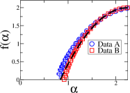
(a) CI, $\Delta_{N}=0.8\pi$

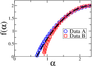
(b) AIII, $\Delta_{A}=0.1\pi$, $\Delta_{N}=0.8\pi$

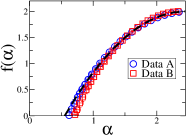
(c) AIII, $\Delta_{A}=0.2\pi$, $\Delta_{N}=0.8\pi$

Figure 15: The $f(\alpha)$ spectra of Dirac fermions with non-Abelian SU(2) vector potential in MFD. Here $\mathcal{N}=40$, $\xi=0.25r$ ($r=L/\mathcal{N}$), and we average over 40 disorder realizations for all three cases. The data are extracted from the numerical derivatives of the IPR. Data A is extracted from binning sizes $b=1$ and $b=2$. Data B is extracted from $b=2$ and $b=4$. The solid lines are the analytical prediction in Eqs. (27) and (31).

VIII Discussion

In this paper we have studied random vector potential Dirac fermions in 2D with one and two valleys. Both cases can be realized as the surface states of bulk topological superconductors.

For the single-valley model, we computed various physical properties for states in the low-energy chiral region, below and above the freezing transition (i.e., for weak and strong disorder). Neither the level statistics nor the two-wavefunction correlations show a qualitative change at the freezing transition. At strong disorder, level statistics remain approximately Wigner-Dyson, and the overlap of the probability distributions for different wavefunctions retains a power-law correlation in energy. The results imply that even the “quasilocalized,” highly rarefied wavefunctions in the strong disorder, frozen regime are correlated in energy and obey generalized Chalker scaling. We want to emphasize that these critically delocalized wavefunctions are not the same as those near the mobility edge.Shklovskii et al. (1993); Kravtsov et al. (1994) The crucial difference is that in the single valley model, all states are delocalized within the low-energy disordered Dirac region, even for strong disorder.

In addition to the low-energy physics of the single-valley model, we also investigated the states away from chiral region. We confirmed that the states at finite energies are delocalized based on their universal multifractal behavior. The multifractal spectrum of these states is well-approximated by that of the integer quantum Hall plateau transition. To our knowledge, this is the first numerical evidence to show the connection between finite-energy states and the plateau transition.

For the two-valley model, we demonstrated that Gade-Wegner scaling does not occur for the AIII class. Our numerical results for the global DoS and the multifractal spectra match well the predictions of conformal field theory.

We discussed two numerical methods, the momentum space Dirac formalism (MFD) and the MDH lattice model. MFD is a way to directly simulate the Dirac fermion problem. It is useful to probe systems with a vanishing DoS and weak multifractality. One can study both low-energy states and states away from the chiral region. MFD is also suitable for simulating multiple valleys and random potentials. The disadvantage is the restriction to relatively small system sizes.

The MDHMotrunich et al. (2002) lattice model is designed for studying single-valley Dirac fermions subject to a static random vector potential. The low-energy theory is described by Eq. (6), with parametrically small mass terms $m_{x,y}$. The low-energy properties including generalized Chalker scaling, the critical behavior of the DoS, and multifractal spectra are consistent with the analytical predictions for the single valley model over a substantial range of $\Delta_{A}$, including the strong disorder regime above the freezing transition. On the other hand, the states far away from the chiral region are Anderson localized. The MDH lattice model might be realizable in artificial materials such as molecular graphene.Gomes et al. (2012) The global DoS and multifractal spectrum of local DoS fluctuations are both experimentally measurable quantities.

We close with open questions and future directions. The surface states for class DIII topological superconductors can also be described by real random vector potential Dirac (Majorana) fermions.Schnyder et al. (2008); Foster et al. ; Xie et al. As in class AIII, it is important to understand whether conformal invariance is preserved for class DIII with three or more valleys.Foster et al. The non-abelian vector potential Dirac fermion in class CI shows universal behavior in the DoS and multifractal spectrum. Constructing a non-abelian version of the MDH model on a lattice might allow the simulation of Dirac fermions with non-abelian vector potentials in artificial materials, and would also allow efficient numerics for much larger system sizes than we could access here using the MFD approach.

We have focused on typical multifractal spectra, obtained by disorder averaging the log of the inverse participation ratio (IPR). The freezing phenomena is related to rare extrema of a typical wavefunction. One can alternatively disorder average the IPR, and then take the log. This gives information about rare configurations of the disorder. It will also be interesting to calculate the disorder-averaged IPR in order to verify the pre-freezing phenomenon.Fyodorov (2009)

IX Acknowledgments

We thank Hong-Yi Xie for discussions on Chalker scaling. This work was supported by the Welch Foundation under Grant No. C-1809.

Appendix A Low Energy Theory of Real Random Hopping $\pi$-Flux Model

We discuss how to derive Dirac fermions in the real random hopping $\pi$-flux model in this appendix. The lattice model belongs to the class BDI in the Altland-Zirnbauer classification.Evers and Mirlin (2008)

We first consider the real random hopping $\pi$-flux model. The Hamiltonian is given by

$$\mathcal{H}=\sum_{\bm{\mathrm{r}}}\Big{[} t_{\bm{\mathrm{r}},\bm{\mathrm{r}}+\hat{x}}(-1)^{\bm{\mathrm{r}}\cdot\hat{y}}c^{\dagger}(\bm{\mathrm{r}})c(\bm{\mathrm{r}}+\hat{x})$$

$$+ t_{\bm{\mathrm{r}},\bm{\mathrm{r}}+\hat{y}}c^{\dagger}(\bm{\mathrm{r}})c(\bm{\mathrm{r}}+\hat{y})+\text{h.c}\Big{]},$$ (33)

The $\pi$-flux lattice contains two sites per unit cell, $\alpha$ and $\beta$. These cannot be chosen in the same way as the sublattice labels $A$ and $B$ shown in Fig. 3. The primitive vectors are $\bm{\mathrm{t}}_{1}=\hat{x}$ and $\bm{\mathrm{t}}_{2}=2\hat{y}$. The lattice constant is set to unity. We label the sites via $\bm{\mathrm{r}}_{\alpha}=(n,2m)$, $\bm{\mathrm{r}}_{\beta}=(n,2m+1)$, with $n,m\in\mathbb{Z}$, and we define $a(\bm{\mathrm{r}}_{\alpha})\equiv c(\bm{\mathrm{r}}_{\alpha})$, and $b(\bm{\mathrm{r}}_{\beta})\equiv c(\bm{\mathrm{r}}_{\beta})$.

In the clean limit ($t_{\bm{\mathrm{r}},\bm{\mathrm{r}}+\hat{x}}=t_{\bm{\mathrm{r}},\bm{\mathrm{r}}+\hat{y}}=t$), the Hamiltonian in momentum space is

$$\mathcal{H}=2t\int_{\bm{\mathrm{k}}\in\text{B.Z.}}\Phi^{\dagger}(\bm{\mathrm{k}})\left[\begin{array}[]{cc}-\cos(k_{x})&\cos(k_{y})\\ \cos(k_{y})&\cos(k_{x})\end{array}\right]\Phi(\bm{\mathrm{k}}),$$

where $\Phi^{\dagger}(\bm{\mathrm{k}})=\left[a^{\dagger}(\bm{\mathrm{k}}),\,\,b^{\dagger}(\bm{\mathrm{k}})\right]$. The dispersion is

$$\omega_{\bm{\mathrm{k}}}=\pm 2t\sqrt{\cos^{2}(k_{x})+\cos^{2}(k_{y})}.$$

The clean $\pi$-flux model can be described by two valleys of decoupled massless Dirac fermions. The distinct Dirac points are $\bm{\mathrm{K}}_{+}=(\frac{\pi}{2},\frac{\pi}{2})$ and $\bm{\mathrm{K}}_{-}=(-\frac{\pi}{2},\frac{\pi}{2})$. The reciprocal vectors of the lattice problem are $\bm{\mathrm{Q}}_{1}=2\pi\hat{x}$ and $\bm{\mathrm{Q}}_{1}=\pi\hat{y}$.

In the low energy limit, only degrees of freedom near the Dirac points play important roles. We therefore use the valley decomposition of the fields,

$$a(\bm{\mathrm{r}}_{\alpha})\approx e^{i\bm{\mathrm{K}}_{+}\cdot\bm{r}_{\alpha}}a_{+}(\bm{\mathrm{r}}_{\alpha})+e^{i\bm{\mathrm{K}}_{-}\cdot\bm{\mathrm{r}}_{\alpha}}a_{-}(\bm{\mathrm{r}}_{\alpha}),$$

$$b(\bm{\mathrm{r}}_{\beta})\approx e^{i\bm{\mathrm{K}}_{+}\cdot\bm{\mathrm{r}}_{\beta}}b_{+}(\bm{\mathrm{r}}_{\beta})+e^{i\bm{\mathrm{K}}_{-}\cdot\bm{\mathrm{r}}_{\beta}}b_{-}(\bm{\mathrm{r}}_{\beta}),$$ (34)

where $+$ and $-$ subscripts specify the low energy degrees of freedom in the vicinity of Dirac points $\bm{\mathrm{K}}_{+}$ and $\bm{\mathrm{K}}_{-}$.

Fermion bilinears that appear in the $\pi$-flux model include $a^{\dagger}(\bm{\mathrm{r}}_{\alpha})a(\bm{\mathrm{r}}_{\alpha}\pm\hat{x})$, $b^{\dagger}(\bm{\mathrm{r}}_{\beta})b(\bm{\mathrm{r}}_{\beta}\pm\hat{x})$, $a^{\dagger}(\bm{\mathrm{r}}_{\alpha})b(\bm{\mathrm{r}}_{\alpha}\pm\hat{y})$, and $b^{\dagger}(\bm{\mathrm{r}}_{\beta})a(\bm{\mathrm{r}}_{\beta}\pm\hat{y})$. We perform the valley decomposition and Taylor expansion for all the bilinears. For example,

$$a^{\dagger}(\bm{\mathrm{r}}_{\alpha}) a(\bm{\mathrm{r}}_{\alpha}\pm\hat{x})+a^{\dagger}(\bm{\mathrm{r}}_{\alpha}\pm\hat{x})a(\bm{\mathrm{r}}_{\alpha})$$

$$\approx i\left[\begin{aligned} &\,a_{+}^{\dagger}(\partial_{x}a_{+})-(\partial_{x}a_{+}^{\dagger})a_{+}\\ &\,-a_{-}^{\dagger}(\partial_{x}a_{-})+(\partial_{x}a_{-}^{\dagger})a_{-}\end{aligned}\right]_{\bm{\mathrm{r}}_{\alpha}}$$

$$\mp(2i)(-1)^{\bm{\mathrm{r}}_{\alpha}\cdot\hat{x}}\left[a^{\dagger}_{+}a_{-}-a^{\dagger}_{-}a_{+}\right]_{\bm{\mathrm{r}}_{\alpha}}.$$

All the bilinear terms contain the staggered factor along the $x$ direction, $(-1)^{\bm{\mathrm{r}}\cdot\hat{x}}$. It suggests that the minimum cell for constructing the low energy theory is a $2$-by-$2$ block.

In the presence of disorder, the hopping terms in Eq. (33) can be viewed as $t_{\bm{\mathrm{r}},\bm{\mathrm{r}}^{\prime}}=t+\delta t_{\bm{\mathrm{r}},\bm{\mathrm{r}}^{\prime}}$, where $\delta t_{\bm{\mathrm{r}},\bm{\mathrm{r}}^{\prime}}$ is a zero-mean random variable. In the clean limit, the low-energy Hamiltonian is

$$\mathcal{H}_{0}=2t\int_{\bm{\mathrm{x}}}\psi^{\dagger}(\bm{\mathrm{x}})\left[-i\sigma_{z}\kappa_{z}\partial_{x}+i\sigma_{x}\partial_{y}\right]\psi(\bm{\mathrm{x}}),$$

where

$$\psi=\left[\begin{array}[]{c}a_{+}\\ b_{+}\\ a_{-}\\ b_{-}\end{array}\right].$$

Here the $\sigma$’s are Pauli matrices acting on ($a/b$) space, and $\kappa$’s are the Pauli matrices on valley ($+/-$) space. The disorder induces the appearance of vector potential and mass terms,

$$\delta\mathcal{H}\approx 2t\int_{\bm{\mathrm{x}}}\psi^{\dagger}\left[A_{x}\sigma_{y}\kappa_{x}+A_{y}\kappa_{y}+m_{x}\sigma_{y}+m_{y}\sigma_{z}\kappa_{y}\right]\psi.$$ (35)

Note that the mass terms $m_{x}$ and $m_{y}$ commute with the vector potential components, but anticommute with the kinetic term.

Now we are in the position to impose the correlated random hopping pattern of the MDH model.Motrunich et al. (2002) The MDH pattern in the $\pi$-flux model is listed below. In a 2-by-2 block associated with position $\bm{\mathrm{R}}$, the hopping elements in Eq. (33) are assigned as

$$t_{\bm{\mathrm{R}},\bm{\mathrm{R}}\pm\hat{x}} =e^{V(\bm{\mathrm{R}})}te^{-V(\bm{\mathrm{R}}\pm\hat{x})},$$

$$t_{\bm{\mathrm{R}},\bm{\mathrm{R}}\pm\hat{y}} =e^{V(\bm{\mathrm{R}})}te^{-V(\bm{\mathrm{R}}\pm\hat{y})},$$

$$t_{\bm{\mathrm{R}}+\hat{y},\bm{\mathrm{R}}+\hat{y}\pm\hat{x}} =e^{V(\bm{\mathrm{R}}+\hat{y}\pm\hat{x})}te^{-V(\bm{\mathrm{R}}+\hat{y})},$$

$$t_{\bm{\mathrm{R}}+\hat{x},\bm{\mathrm{R}}+\hat{x}\pm\hat{y}} =e^{V(\bm{\mathrm{R}}+\hat{x}\pm\vec{y})}te^{-V(\bm{\mathrm{R}}+\hat{x})},$$

where $\bm{\mathrm{R}}=(2n,2m)$, $n$ and $m$ are integers. $V(\bm{\mathrm{y}})$ is a random surface obeying Eq. (8). The low energy theory for the MDH model on $\pi$-flux lattice is given by

$$\mathcal{H}=\mathcal{H}_{0}+2t\int_{\bm{\mathrm{x}}}\psi^{\dagger}\left[(\partial_{y}V)\sigma_{y}\kappa_{x}+(\partial_{x}V)\kappa_{y}\right]\psi.$$

The mass terms in Eq. (35) vanish up to second order derivatives in $V$, after we we coarse grain a 2-by-2 block in the lattice model at each position $\bm{\mathrm{R}}$.

The derived low energy theory is nothing but Eq. (6) after applying the following basis rotation,

$$\psi\rightarrow\frac{1}{\sqrt{2}}\left(1+i\sigma_{x}\kappa_{z}\right)\frac{1}{\sqrt{2}}\left(1+i\kappa_{y}\right)\frac{1}{\sqrt{2}}\left(1+i\sigma_{z}\right)\psi.$$

As a comparison, we also briefly discuss the MDH model on the honeycomb lattice. The hopping amplitudes can be generated via Eq. (9). The low energy theory reads

$$\mathcal{H}\approx\frac{3t}{2}\int_{\bm{\mathrm{x}}}\psi^{\dagger}\left[-i\sigma_{x}\partial_{x}-i\sigma_{y}\partial_{y}+\bm{\mathrm{A}}\cdot\bm{\mathrm{\sigma}}\mu_{z}\right]\psi,$$

where the basis convention for the honeycomb lattice is

$$\psi=\left[\begin{array}[]{c}a_{+}\\ b_{+}\\ b_{-}\\ -a_{-}\end{array}\right]$$ (40)

($a$ and $b$ label the triangular sublattices).

The mass terms are related to the Kekulé patterns in the honeycomb latticeHou et al. (2007). A minimum 6-site hexagon is needed for performing the coarse graining procedure contrary to a 4-site square block for $\pi$-flux lattice. In this aspect, the MDH model on the honeycomb lattice will require a larger system in order to avoid deviations generated by non-zero masses. This is consistent with what we report for the numerical DoS in Fig. 6, where results obtained for the MDH $\pi$-flux and honeycomb lattices are compared for equal system sizes.

Appendix B Random phase Disorder

In this appendix we discuss our parametrization of the disorder potentials employed in this paper. In particular, we show how to realize the correlated disorder with the random phase method (discussed below). Consider a real-valued disorder potential, $B(\bm{\mathrm{x}})$, satisfying

$$\langle B(\bm{\mathrm{x}})\rangle_{\text{dis}} =0,$$ (41)

$$\langle B(\bm{\mathrm{x}}+\bm{\mathrm{R}})B(\bm{\mathrm{x}})\rangle_{\text{dis}} =\Delta_{B}\,\mathcal{K}(\bm{\mathrm{R}}),$$ (42)

where $\langle\dots\rangle_{\text{dis}}$ denotes disorder average, $\Delta_{B}$ indicates the strength of the disorder potential, and $\mathcal{K}(\bm{R})$ is a normalized real-valued distribution in the position space.

In the infinite size limit, one can exchange the disorder average $\langle\dots\rangle_{\text{dis}}$ by the spatial average $\langle\dots\rangle_{\bm{x}}$. In a finite system, we need to be careful about which scheme is employed. For Gaussian correlated disorder $G(\bm{\mathrm{x}})$ in 2D, one can parametrize the potential in terms of randomly positioned impurities with a Gaussian scattering profile,Bardarson et al. (2007); Nomura and MacDonald (2007)

$$G(\bm{\mathrm{x}})=\frac{1}{2\pi s^{2}}\left[\sum_{j=1}^{N_{+}}e^{-\frac{\left(\bm{\mathrm{x}}-\bm{\mathrm{y}}^{+}_{j}\right)^{2}}{2s^{2}}}-\sum_{j=1}^{N_{-}}e^{-\frac{(\bm{\mathrm{x}}-\bm{\mathrm{y}}^{-}_{j})^{2}}{2s^{2}}}\right].$$

In this equation, the $\bm{\mathrm{y}}$’s indicate the positions of the impurities, and $N_{+}$ and $N_{-}$ are the numbers of positive charged and negative charged impurities. The disorder profile is determined by the configuration of the $\bm{\mathrm{y}}$’s. For the zero mean case, we choose $N_{+}=N_{-}=N$. The $G(\bm{\mathrm{x}})$ generated in this way satisfies the following properties:

$$\langle G(\bm{\mathrm{x}})\rangle_{\{\bm{\mathrm{y}}\}} =0,$$

$$\langle G(\bm{\mathrm{x}}+\bm{\mathrm{R}})G(\bm{\mathrm{x}})\rangle_{\{\bm{\mathrm{y}}\}} =\frac{2N_{+}}{L^{2}}\left[\frac{1}{2\pi(\sqrt{2}s)^{2}}e^{-\frac{\bm{\mathrm{R}}^{2}}{2(\sqrt{2}s)^{2}}}-\frac{1}{L^{2}}\right],$$

where

$$\langle f(\{\bm{\mathrm{y}}\})\rangle_{\{\bm{\mathrm{y}}\}}\equiv\prod_{i}\left[\frac{1}{L^{2}}\int d^{2}\bm{\mathrm{y}}_{i}\right]f(\{\bm{\mathrm{y}}\}).$$

The strength of the disorder potential is determined by the total density of the scatters $2N/L^{2}$. Moreover, there is a $\sqrt{2}$-enhancement in the resultant Gaussian correlation length.

In a fixed disorder realization, the Fourier components of $G(\bm{\mathrm{x}})$ are given by

$$\widetilde{G}_{\bm{\mathrm{m}}\neq(0,0)}=e^{-\frac{1}{2}(\frac{2\pi}{L}\bm{\mathrm{m}}s)^{2}}\left[\sum_{j=1}^{N}e^{i\frac{2\pi}{L}\bm{\mathrm{m}}\cdot\bm{\mathrm{y^{+}_{j}}}}-\sum_{j=1}^{N}e^{i\frac{2\pi}{L}\bm{\mathrm{m}}\cdot\bm{\mathrm{y^{-}_{j}}}}\right].$$

When $N$ is sufficiently large, the term in square brackets can be approximated by a random phase term

$$\left[\sum_{j=1}^{N}e^{i\frac{2\pi}{L}\bm{\mathrm{m}}\cdot\bm{\mathrm{y^{+}_{j}}}}-\sum_{j=1}^{N}e^{i\frac{2\pi}{L}\bm{\mathrm{m}}\cdot\bm{\mathrm{y^{-}_{j}}}}\right]\approx\sqrt{2N}e^{i\phi_{\bm{\mathrm{m}}}},$$ (43)

where $\phi_{-\bm{\mathrm{m}}}=-\phi_{\bm{\mathrm{m}}}$ for $\bm{\mathrm{m}}\neq\bm{\mathrm{0}}$.

The scheme discussed above is limited to certain specific correlation profiles. For the long-ranged correlated disorder potentials in Eq. (8), one needs to use a more general approach to generate randomness.

In the rest of the appendix, we focus on constructing disorder potentials by assigning random phases. Instead of working with the conditions in Eqs. (41) and (42) directly, we replace the disorder average by the spatial average. Therefore, $B(\bm{\mathrm{x}})$ satisfies

$$\langle B(\bm{\mathrm{x}})\rangle_{\bm{\mathrm{x}}} =0,$$ (44)

$$\langle B(\bm{\mathrm{x}}+\bm{\mathrm{R}})B(\bm{\mathrm{x}})\rangle_{\bm{\mathrm{x}}} =\Delta_{B}\mathcal{K}(\bm{\mathrm{R}}),$$ (45)

where

$$\langle f(\bm{\mathrm{x}})\rangle_{\bm{\mathrm{x}}}\equiv L^{-2}\int d^{2}{\bm{\mathrm{x}}}\,f(\bm{\mathrm{x}}).$$

The zero-mean condition [Eq. (44)] indicates that $\widetilde{B}_{\bm{\mathrm{n}}=\bm{\mathrm{0}}}$ vanishes, where $\widetilde{B}_{\bm{\mathrm{n}}}$ is the Fourier component of $B(\bm{\mathrm{x}})$. The condition in Eq. (45),

$$\langle B(\bm{\mathrm{x}})B(\bm{\mathrm{x}}+\bm{R})\rangle_{\bm{\mathrm{x}}}=\Delta_{B}\mathcal{K}(\bm{\mathrm{R}})$$

$$\rightarrow \frac{1}{L^{4}}\sum_{\bm{\mathrm{m}}}e^{i\Delta_{k}\bm{\mathrm{m}}\cdot\bm{\mathrm{R}}}\widetilde{B}_{-\bm{\mathrm{m}}}\widetilde{B}_{\bm{\mathrm{m}}}=\frac{\Delta_{B}}{L^{2}}\sum_{\bm{\mathrm{m}}}e^{i\Delta_{k}\bm{\mathrm{m}}\cdot\bm{\mathrm{R}}}\widetilde{\mathcal{K}}_{\bm{\mathrm{m}}}$$

$$\rightarrow \widetilde{B}_{-\bm{\mathrm{m}}}\,\widetilde{B}_{\bm{\mathrm{m}}}=\left|\widetilde{B}_{\bm{\mathrm{m}}}\right|^{2}=L^{2}\Delta_{B}\widetilde{\mathcal{K}}_{\bm{\mathrm{m}}}$$

where we have used $\widetilde{B}_{\bm{\mathrm{m}}}^{*}=\widetilde{B}_{-\bm{\mathrm{m}}}$.

Assuming that $\widetilde{\mathcal{K}}_{\bm{\mathrm{m}}}$ is real and non-negative, the disorder potential in the momentum space satisfies

$$\widetilde{B}_{\bm{\mathrm{m}}=0} =0,$$

$$\widetilde{B}_{\bm{\mathrm{m}}\neq 0} =L\sqrt{\Delta_{B}}\left(\widetilde{\mathcal{K}}_{\bm{\mathrm{m}}}\right)^{\frac{1}{2}}e^{i\theta_{\bm{\mathrm{m}}}},$$

where $\theta_{\bm{\mathrm{m}}}$ is an uniform random variable from $0$ to $2\pi$ and $\theta_{-\bm{\mathrm{m}}}=-\theta_{\bm{\mathrm{m}}}$. The disorder average can be performed by averaging over $\theta$’s. The potential $B(\bm{\mathrm{x}})$ constructed this way satisfies the following equations:

$$\langle B(\bm{\mathrm{x}})\rangle_{\{\theta\}} =0,$$

$$\langle B(\bm{\mathrm{x}}+\bm{\mathrm{R}})B(\bm{\mathrm{x}})\rangle_{\{\theta\}} =\Delta_{B}\left[\mathcal{K}(\bm{\mathrm{R}})-\frac{1}{L^{2}}\right],$$

where

$$\langle f(\{\theta\})\rangle_{\{\theta\}}=\prod_{i}\left[\int_{0}^{2\pi}\frac{d\theta_{i}}{2\pi}\right]f(\{\theta\}).$$

The $\prod_{i}$ in the above equation runs over all the independent $\theta_{i}$. The configuration of $\theta_{\bm{\mathrm{m}}}$ characterizes the disordered potential. The finite size correction is similar to the random-position impurity scheme discussed earlier.

The random phase method is particularly efficient in the MFD scheme because the randomness is directly assigned to the Fourier mode, rather than the position space profile. This scheme also allows us to simulate Eq. (8).

References

- Anderson (1958) P. W. Anderson, Phys. Rev. 109, 1492 (1958).
- (2) D. A. Huse and V. Oganesyan, arXiv:1305.4915.
- Basko et al. (2006) D. Basko, I. Aleiner, and B. Altshuler, Annals of Physics 321, 1126 (2006).
- Oganesyan and Huse (2007) V. Oganesyan and D. A. Huse, Phys. Rev. B 75, 155111 (2007).
- Pal and Huse (2010) A. Pal and D. A. Huse, Phys. Rev. B 82, 174411 (2010).
- Sivan and Imry (1987) U. Sivan and Y. Imry, Phys. Rev. B 35, 6074 (1987).
- Chalker and Daniell (1988) J. T. Chalker and G. J. Daniell, Phys. Rev. Lett. 61, 593 (1988).
- Chalker (1990) J. Chalker, Physica A: Statistical Mechanics and its Applications 167, 253 (1990).
- Fyodorov and Mirlin (1997) Y. V. Fyodorov and A. D. Mirlin, Phys. Rev. B 55, R16001 (1997).
- Cuevas and Kravtsov (2007) E. Cuevas and V. E. Kravtsov, Phys. Rev. B 76, 235119 (2007).
- Huckestein (1995) B. Huckestein, Rev. Mod. Phys. 67, 357 (1995).
- Evers and Mirlin (2008) F. Evers and A. D. Mirlin, Rev. Mod. Phys. 80, 1355 (2008).
- Chamon et al. (1996) C. C. Chamon, C. Mudry, and X.-G. Wen, Phys. Rev. Lett. 77, 4194 (1996).
- Ryu and Hatsugai (2001a) S. Ryu and Y. Hatsugai, Phys. Rev. B 63, 233307 (2001a).
- Carpentier and Le Doussal (2001) D. Carpentier and P. Le Doussal, Phys. Rev. E 63, 026110 (2001).
- (16) G. Biroli, A. C. Ribeiro-Teixeira, and M. Tarzia, arXiv:1211.7334.
- (17) A. D. Luca, A. Scardicchio, V. E. Kravtsov, and B. L. Altshuler, arXiv:1401.0019.
- de Luca and Scardicchio (2013) A. de Luca and A. Scardicchio, Eur. Phys. Lett. 101, 37003 (2013).
- Dobrosavljević et al. (2012) V. Dobrosavljević, N. Trivedi, and J. M. Valles, Conductor-Insulator Quantum Phase Transitions (Oxford University Press, Oxford, 2012).
- Schnyder et al. (2008) A. P. Schnyder, S. Ryu, A. Furusaki, and A. W. W. Ludwig, Phys. Rev. B 78, 195125 (2008).
- Foster and Yuzbashyan (2012) M. S. Foster and E. A. Yuzbashyan, Phys. Rev. Lett. 109, 246801 (2012).
- Hosur et al. (2010) P. Hosur, S. Ryu, and A. Vishwanath, Phys. Rev. B 81, 045120 (2010).
- Ludwig et al. (1994) A. W. W. Ludwig, M. P. A. Fisher, R. Shankar, and G. Grinstein, Phys. Rev. B 50, 7526 (1994).
- Motrunich et al. (2002) O. Motrunich, K. Damle, and D. A. Huse, Phys. Rev. B 65, 064206 (2002).
- Gomes et al. (2012) K. K. Gomes, W. Mar, W. Ko, F. Guinea, and H. C. Manoharan, Nature 483, 306 (2012).
- Hatsugai et al. (1997) Y. Hatsugai, X.-G. Wen, and M. Kohmoto, Phys. Rev. B 56, 1061 (1997).
- Morita and Hatsugai (1997) Y. Morita and Y. Hatsugai, Phys. Rev. Lett. 79, 3728 (1997).
- Ryu and Hatsugai (2001b) S. Ryu and Y. Hatsugai, Phys. Rev. B 65, 033301 (2001b).
- Chen et al. (2012) X. Chen, B. Hsu, T. L. Hughes, and E. Fradkin, Phys. Rev. B 86, 134201 (2012).
- Nersesyan et al. (1994) A. A. Nersesyan, A. M. Tsvelik, and F. Wenger, Phys. Rev. Lett. 72, 2628 (1994).
- Castillo et al. (1997) H. E. Castillo, C. C. Chamon, E. Fradkin, P. M. Goldbart, and C. Mudry, Phys. Rev. B 56, 10668 (1997).
- Horovitz and Doussal (2002) B. Horovitz and P. LeDoussal, Phys. Rev. B 65, 125323 (2002).
- Mudry et al. (2003) C. Mudry, S. Ryu, and A. Furusaki, Phys. Rev. B 67, 064202 (2003).
- Huckestein and Schweitzer (1994) B. Huckestein and L. Schweitzer, Phys. Rev. Lett. 72, 713 (1994).
- Pracz et al. (1996) K. Pracz, M. Janssen, and P. Freche, Journal of Physics: Condensed Matter 8, 7147 (1996).
- Kravtsov et al. (2010) V. E. Kravtsov, A. Ossipov, O. M. Yevtushenko, and E. Cuevas, Phys. Rev. B 82, 161102 (2010).
- Ostrovsky et al. (2007) P. M. Ostrovsky, I. V. Gornyi, and A. D. Mirlin, Phys. Rev. Lett. 98, 256801 (2007).
- Nomura et al. (2008) K. Nomura, S. Ryu, M. Koshino, C. Mudry, and A. Furusaki, Phys. Rev. Lett. 100, 246806 (2008).
- Mudry et al. (1996) C. Mudry, C. Chamon, and X.-G. Wen, Nucl. Phys. B 466, 383 (1996).
- Caux et al. (1996) J.-S. Caux, I. Kogan, and A. Tsvelik, Nucl. Phys. B 466, 444 (1996).
- Ostrovsky et al. (2006) P. M. Ostrovsky, I. V. Gornyi, and A. D. Mirlin, Phys. Rev. B 74, 235443 (2006).
- (42) H.-Y. Xie, Y.-Z. Chou, and M. S. Foster, in preparation.
- Castro Neto et al. (2009) A. H. Castro Neto, F. Guinea, N. M. R. Peres, K. S. Novoselov, and A. K. Geim, Rev. Mod. Phys. 81, 109 (2009).
- Das Sarma et al. (2011) S. Das Sarma, S. Adam, E. H. Hwang, and E. Rossi, Rev. Mod. Phys. 83, 407 (2011).
- Hasan and Kane (2010) M. Z. Hasan and C. L. Kane, Rev. Mod. Phys. 82, 3045 (2010).
- Qi and Zhang (2011) X.-L. Qi and S.-C. Zhang, Rev. Mod. Phys. 83, 1057 (2011).
- Foster and Ludwig (2008) M. S. Foster and A. W. W. Ludwig, Phys. Rev. B 77, 165108 (2008).
- (48) M. S. Foster, H.-Y. Xie, and Y.-Z. Chou, Phys. Rev. B 89, 155140 (2014).
- Nomura and MacDonald (2007) K. Nomura and A. H. MacDonald, Phys. Rev. Lett. 98, 076602 (2007).
- Bardarson et al. (2007) J. H. Bardarson, J. Tworzydło, P. W. Brouwer, and C. W. J. Beenakker, Phys. Rev. Lett. 99, 106801 (2007).
- Gade and Wegner (1991) R. Gade and F. Wegner, Nucl. Phys. B 360, 213 (1991).
- Gade (1993) R. Gade, Nucl. Phys. B 398, 499 (1993).
- Hou et al. (2007) C.-Y. Hou, C. Chamon, and C. Mudry, Phys. Rev. Lett. 98, 186809 (2007).
- (54) The chosen value of the correlation length relates the former to the fixed inverse ultraviolet cutoff . The latter would be set relative to the lattice spacing in a microscopic model. The value of should be small compared to the system size , but finite because the Gaussian correlation is a regularization of the white-noise condition in Eq. (3b). A slightly smaller or larger ratio than gives the same result; this is a stable parameter region.
- (55) The mass terms in the low energy theory are scaled with , up to logarithmic corrections in .
- Richardella et al. (2010) A. Richardella, P. Roushan, S. Mack, B. Zhou, D. A. Huse, D. D. Awschalom, and A. Yazdani, Science 327, 665 (2010).
- Mirlin (2000) A. D. Mirlin, Phys. Rep. 326, 259 (2000).
- Evangelou and Katsanos (2003) S. N. Evangelou and D. E. Katsanos, Journal of Physics A: Mathematical and General 36, 3237 (2003).
- Evers et al. (2001) F. Evers, A. Mildenberger, and A. D. Mirlin, Phys. Rev. B 64, 241303 (2001).
- Evers et al. (2008) F. Evers, A. Mildenberger, and A. D. Mirlin, Phys. Rev. Lett. 101, 116803 (2008).
- Obuse et al. (2008) H. Obuse, A. R. Subramaniam, A. Furusaki, I. A. Gruzberg, and A. W. W. Ludwig, Phys. Rev. Lett. 101, 116802 (2008).
- Schnyder et al. (2009) A. P. Schnyder, S. Ryu, and A. W. W. Ludwig, Phys. Rev. Lett. 102, 196804 (2009).
- Nersesyan et al. (1995) A. Nersesyan, A. Tsvelik, and F. Wenger, Nucl. Phys. B 438, 561 (1995).
- Di Francesco et al. (1996) P. Di Francesco, P. Mathieu, and D. Sènèchal, Conformal Field Theory (Springer-Verlag, New York, 1996).
- Witten (1984) E. Witten, Comm. Math. Phys. 92, 455 (1984).
- Guruswamy et al. (2000) S. Guruswamy, A. LeClair, and A. Ludwig, Nucl. Phys. B 583, 475 (2000).
- Tsvelik (1995) A. M. Tsvelik, Phys. Rev. B 51, 9449 (1995).
- Shklovskii et al. (1993) B. I. Shklovskii, B. Shapiro, B. R. Sears, P. Lambrianides, and H. B. Shore, Phys. Rev. B 47, 11487 (1993).
- Kravtsov et al. (1994) V. E. Kravtsov, I. V. Lerner, B. L. Altshuler, and A. G. Aronov, Phys. Rev. Lett. 72, 888 (1994).
- Fyodorov (2009) Y. V. Fyodorov, Journal of Statistical Mechanics: Theory and Experiment 2009, P07022 (2009).