Local Electronic Structure around a Single Impurity in an Anderson Lattice Model for Topological Kondo Insulators

Abstract

Shortly after the discovery of topological band insulators, the topological Kondo insulators (TKIs) have also been theoretically predicted. The latter has ignited revival interest in the properties of Kondo insulators. Currently, the feasibility of topological nature in SmB₆ has been intensively analyzed by several complementary probes. Here by starting with a minimal-orbital Anderson lattice model, we explore the local electronic structure in a Kondo insulator. We show that the two strong topological regimes sandwiching the weak topological regime give rise to a single Dirac cone, which is located near the center or corner of the surface Brillouin zone. We further find that, when a single impurity is placed on the surface, low-energy resonance states are induced in the weak scattering limit for the strong TKI regimes and the resonance level moves monotonically across the hybridization gap with the strength of impurity scattering potential; while low energy states can only be induced in the unitary scattering limit for the weak TKI regime, where the resonance level moves universally toward the center of the hybridization gap. These impurity induced low-energy quasiparticles will lead to characteristic signatures in scanning tunneling microscopy/spectroscopy, which has recently found success in probing into exotic properties in heavy fermion systems.

I Introduction

Topological insulators (TIs) are a novel state of matter. MZHasan:2010 ; XLQi:2010 ; XLQi:2011 Different from conventional band insulators, the new class of materials exhibit not only a bulk insulating band gap but also gapless spin-filtered edge states in two-dimensions or a metallic Dirac fermion surface states in three dimensions. So far, the compounds HgTe, Bi₂Se₃, Bi_1-xSb_x, Bi₂Te₃, and TlBiTe₂ have been identified as weakly interacting TIs, YXia:2009 ; PRoushan:2009 ; TZhang:2009 ; JSeo:2010 ; ZAlpichshev:2010 where the band inversion is driven by the spin-orbit coupling BABernevig:2006 . The main complication in these band insulators (especially Bi-based compounds) is that they still have a high concentration of bulk carriers, giving rise to a considerable residual conductivity in the sample bulk. Soon after their discovery, the possibility of interaction driven topological insulators SRaghu:2008 ; KSun:2009 ; RNandkishore:2010 ; KSun:2012 ; HMGuo:2009 ; DAPesin:2010 ; XWan:2011 ; BJYang:2010 ; MDzero:2010 ; XZhang:2012 ; BYan:2012 ; MDzero:2012 ; MTTran:2012 ; FLu:2013 ; XDeng:2013 ; VAlexandrov:2013 ; XYFeng:2013 has been discussed in the context that the bulk insulating behavior may be enhanced by the interplay between electron correlation and spin-orbit coupling. In particular, there has been intensified interest in the possibility of topological Kondo insulators in $f$-electron materials. Kondo insulators are a type of heavy fermion materials that have been studied for nearly four decades. In these materials, the on-site Coulomb repulsion on localized $f$-electrons significantly renormalizes the $f$-electron band width. Theoretically, the idea of TKIs has been first proposed by Coleman and co-workers, who showed that Kondo insulators could develop topologically nontrival ground states, which are connected adiabatically to those in noninteracting insulators. MDzero:2010 The proposal has sparked a flurry of experimental attempts to demonstrate the existence of topological surface states on a prototype of Kondo insulators, SmB₆, which is a stoichiometric compound (distinct from the topological band insulators as mentioned above) and has recently been suggested to be a class of topological Kondo insulators (TKIs). TTakimoto:2011 On the one hand, the notion of TKI has been adopted to explain results from several transport, SWolgast:2013 ; ZJYue:2013 de Haas-van Alphen effect, GLi:2013 angle-resolved photoemission spectroscopy, NXu:2013 ; MNeupane:2013 ; JJiang:2013 and scanning tunneling microscopy (STM) MMYee:2013 experiments. On the other hand, the ARPES has not unanimously agreed upon the associated Dirac cones while it has also been proposed that the resistivity in SmB₆ can arise through native surface instabilities such as a non-TI metallic surface states, ZHZhu:2013 a band inversion layer, EFrantzeskakis:2013 or surface reconstruction. SRobler:2013 Therefore, more theoretical and experimental efforts are needed to uncover the features manifesting the topological aspect of SmB₆ in particular and other interesting Kondo insulators in general. The use of single impurity with the STM technique has proved to be a powerful approach to distinguish the nature of underlying electronic states in strongly correlated electron systems. It has been used to identify the pairing symmetry in unconventional superconductors, AVBalatsky:2006 ; JXZhu:2011 ; CLSong:2013 and to shed insight into the hidden order state in URu₂Si₂. MHHamidian:2011 In this work, we propose to study the local electronic structure around a single impurity on the surface of a topological Kondo insulator. Within the Gutzwiller method, we are able to establish the necessary condition for the existence of a bulk energy gap near the Fermi energy. We further find that the existence of impurity induced bound state is sensitive to the potential strength. This dependence is unique to the topological nature of the Kondo insulator state, out of which the surface metallic state emerge. The prediction should be readily accessible to the STM experiments, in view of the recent success of this technique applied to understand the bulk and surface properties of SmB₆. MMYee:2013 ; SRobler:2013

The outline of this work is as follows: We start with a generalized Anderson lattice model and discuss the Gutzwiller variational wavefunction approach in Sec. II. The characterization of $Z_{2}$ topological indices and the $T$-matrix method for the calculation of local electronic structure around a nonmagnetic impurity are presented in the same section. In Sec. III, the dependence of the topological properties on the model parameter is studied. The relation between the number of Dirac cone in the surface Brillouin zone and the topological indices is discussed. Furthermore, the existence of the low-energy quasiparticle states around a single impurity is elucidated in both strong and weak topological insulator regimes. A summary is given in Sec. IV.

II Theoretical Methods

Our starting point is a generalized periodic Anderson model

$$H=H_{0}+H_{\text{imp}}\;.$$ (1)

The term on the right-hand side (RHS) of Eq. (1), $H_{0}$, describes the pristine bulk or slab structure of the heavy fermion system and consists of three parts:

$$H_{c}=-\sum_{ij,\sigma}(t_{ij}^{c}+\mu\delta_{ij})c_{i\sigma}^{\dagger}c_{j\sigma}\;,$$ (2a)

for the conduction electrons,

$$H_{f}=\sum_{i,\alpha}(\epsilon_{f}-\mu)f_{i\alpha}^{\dagger}f_{i\alpha}+\sum_{i}U_{f}n_{i\uparrow}^{f}n_{i\downarrow}^{f}+(J_{H}/2)\sum_{ij}\mathbf{S}_{i}\cdot\mathbf{S}_{j}\;,$$ (2b)

for local $$f$$-electrons, and

$$H_{hyb}=\sum_{ij,\sigma\alpha}[c_{i\sigma}^{\dagger}V_{cf,ij,\sigma\alpha}f_{j\alpha}+\text{H.c.}]\;,$$ (2c)

for hybridization between the conduction and $$f$$-electrons.

The second term on the RHS of Eq. (1),

$$H_{\text{imp}}=\sum_{\alpha}U_{imp}f_{0\alpha}^{\dagger}f_{0\alpha}\;,$$ (3)

describes the single-site impurity scattering, which without loss of generality is located at the origin of the lattice coordinate system. Here the operators $c_{i\sigma}^{\dagger}$ ($c_{i\sigma}$) create (annihilate) a conduction electron at site $\mathbf{r}_{i}$ with spin projection $\sigma$ while the operators $f_{i\alpha}^{\dagger}$ ($f_{i\alpha}$) create (annihilate) a $f$-level electron at site $\mathbf{r}_{i}$ with pseudo-spin projection $\alpha$ representing the $\Gamma_{8(2),+}$ and $\Gamma_{8(2),-}$ components due to strong spin-orbit coupling. MTTran:2012 The number operators for $c$ and $f$ orbitals with spin projection are given by $n_{i\sigma}^{c}=c_{i\sigma}^{\dagger}c_{i\sigma}$ and $n_{i\alpha}^{f}=f_{i\alpha}^{\dagger}f_{i\alpha}$, respectively. The quantity $t_{ij}^{c}$ is the hopping integral of the conduction electrons, $\epsilon_{f}$ is the local $f$-orbital energy level on the magnetic atoms, and $\mu$ is the chemical potential. The hybridization matrix between the conduction band and $f$-orbital on the magnetic atoms is represented by $V_{cf,ij}$ and the $f$-electrons on the magnetic atoms experience the Coulomb repulsion of strength $U_{f}$. For a simple cubic lattice, by considering the hybridization between 6$s$ and 4$f$ electrons of rare-earth systems in the limit of strong spin-orbit coupling for the $f$-electrons, one can model the nearest-neighbor three-dimensional hybridization in the form: MTTran:2012

$$V_{cf,ij}=\mathbf{d}_{ij}\cdot\bm{\sigma}\;.$$ (4)

Here $\bm{\sigma}$ is the Pauli matrix and $\mathbf{d}_{ij}=(V_{x}d_{ij}^{x},V_{y}d_{ij}^{y},V_{z}d_{ij}^{z})$, where $V_{x}=V_{y}=V_{z}/2=V_{cf}$, while $d_{ij}^{x}=\delta_{i_{y},j_{y}}\delta_{i_{z},j_{z}}(x_{i}-x_{j})/a$, $d_{ij}^{x}=-\delta_{i_{x},j_{x}}\delta_{i_{z},j_{z}}(y_{i}-y_{j})/a$, and $d_{ij}^{z}=-\delta_{i_{x},j_{x}}\delta_{i_{y},i_{y}}(z_{i}-z_{j})/a$. The quantity $a$ is the lattice constant of the simple cubit system. We note that although for the typical systems like SmB₆, the dominant hybridization could occur between 5$d$ and 4$f$ orbitals, the hybridization structure should be similar and the essential physics as described in the present work should be robust. In addition, we have also introduced a Ruderman-Kittel-Kasuya-Yoshida (RKKY) type pseudo spin interactions to describe the spin liquid. TSenthil:2003 ; TSenthil:2004 ; CPepin:2007 ; JXZhu:2008 This type of effective models have been most studied for the non-Fermi-liquid physics near the heavy-fermion quantum criticality. PGegenwart:2008 We generalize the Gutzwiller approximation JXZhu:2012 to solve the pristine part of the Hamiltonian $H_{0}$ and proceed to study the local electronic structure around the single impurity within the $T$-matrix method. AVBalatsky:2006

II.1 Gutzwiller approximation method

Due to the presence of onsite Hubbard interaction $U_{f}$ between the $f$-electrons on each lattice site in Eq. (1), the problem even for the pristine system $H_{0}$ is already strongly correlated. This strong correlation effect can be accounted for by reducing the statistical weight of double occupation in the Gutzwiller projected wavefunction approach, MCGutzwiller:1963 and the projection can be carried out semi-analytically within the Gutzwiller approximation. MCGutzwiller:1965 ; DVollhardt:1984 ; FCZhang:1988 In the present problem, the lattice translation symmetry is already broken in the stab geometry, we thus use a spatially unrestricted Gutzwiller approximation CLi:2006 ; JPJulien:2006 ; QHWang:2006 ; WHKo:2007 ; NFukushima:2008 to translate the Hamiltonian $H_{0}$ for the pristine system into the following renormalized mean-field Hamiltonian:

$$H_{\text{eff},0} = -\sum_{ij,\sigma}(t_{ij}^{c}+\mu\delta_{ij})c_{i\sigma}^{\dagger}c_{j\sigma}+\sum_{ij,\sigma\alpha}[V_{cf,ij,\sigma\alpha}g_{t,j\alpha}c_{i\sigma}^{\dagger}\tilde{f}_{i\alpha}+\text{H.c.}]+\sum_{i,\alpha}(\epsilon_{f}+\lambda_{i}-\mu)\tilde{f}_{i\alpha}^{\dagger}\tilde{f}_{i\alpha}$$ (5)

$$-\frac{3J_{H}}{4}\sum_{ij,\alpha}g_{s,i}g_{s,j}\tilde{\chi}_{ij}\tilde{f}_{i\alpha}^{\dagger}\tilde{f}_{j\alpha}+\sum_{i}U_{f}d_{i}\;,$$

where $\lambda_{i}$ and $d_{i}$ are the Lagrange multiplier and the double occupation at site $i$. We have used $\tilde{f}_{i\alpha}^{\dagger}$ ($\tilde{f}_{i\alpha}$) to denote the quasiparticle field operators to differentiate from the truly $f$-electron operators in Eq. (1). The spin liquid term is described by the resonant valence bond order $\tilde{\chi}_{ij}=\sum_{\alpha}\tilde{f}_{i\alpha}^{\dagger}\tilde{f}_{j\alpha}/2$. The local $c$-$f$ hybridization and spin-exchange interaction have been renormalized by a factor of $g_{t,i\alpha}$ and $g_{s,i}g_{s,j}$, respectively. These $g$ factors are given by

$$g_{t,i\alpha}=\biggl{[}\frac{(\bar{n}_{i\alpha}^{\tilde{f}}-d_{i})(1-\bar{n}_{i}^{\tilde{f}}+d_{i})}{\bar{n}_{i\alpha}^{\tilde{f}}(1-\bar{n}_{i\alpha}^{\tilde{f}})}\biggr{]}^{1/2}+\biggl{[}\frac{d_{i}(\bar{n}_{i\bar{\alpha}}^{\tilde{f}}-d_{i})}{\bar{n}_{i\alpha}^{\tilde{f}}(1-\bar{n}_{i\alpha}^{\tilde{f}})}\biggr{]}^{1/2}\;,$$ (6)

and

$$g_{s,i}=\biggl{[}\frac{(\bar{n}_{i\bar{\alpha}}^{\tilde{f}}-d_{i})(\bar{n}_{i\alpha}^{\tilde{f}}-d_{i})}{\bar{n}_{i\bar{\alpha}}^{\tilde{f}}(1-\bar{n}_{i\alpha}^{\tilde{f}})\bar{n}_{i\alpha}^{\tilde{f}}(1-\bar{n}_{i\bar{\alpha}}^{\tilde{f}})}\biggr{]}^{1/2}\;.$$ (7)

Here $\bar{n}_{i\alpha}^{\tilde{f}}$ being the expectation value of the pseudo spin-$\alpha$ density operator $n_{i\alpha}^{\tilde{f}}=\tilde{f}_{i\alpha}^{\dagger}\tilde{f}_{i\alpha}$ and $\bar{n}_{i}^{\tilde{f}}=\sum_{\alpha}\bar{n}_{i\alpha}^{\tilde{f}}$. Minimization of the expectation value of $H_{\text{eff},0}$ leads to the following self-consistency conditions for $\lambda_{i}$ and $d_{i}$:

$$\lambda_{i} = \frac{1}{2}\biggl{(}\frac{\partial g_{t,i\uparrow}}{\partial\bar{n}_{i\uparrow}^{\tilde{f}}}+\frac{\partial g_{t,i\uparrow}}{\partial\bar{n}_{i\downarrow}^{\tilde{f}}}\biggl{)}\sum_{j,\sigma\alpha}[\mathbf{d}_{ji}\cdot\bm{\sigma}_{\sigma\alpha}\langle c_{j\sigma}^{\dagger}\tilde{f}_{i\alpha}\rangle+\text{c.c}]-\frac{3J_{H}}{4}\biggl{(}\frac{\partial g_{s,i}}{\partial\bar{n}_{i\uparrow}^{\tilde{f}}}+\frac{\partial g_{s,i}}{\partial\bar{n}_{i\downarrow}^{\tilde{f}}}\biggr{)}\sum_{j}g_{s,j}|\tilde{\chi}_{ij}|^{2}\;,$$ (8a)

$$-U_{f} = \sum_{j,\sigma\alpha}\biggl{[}\mathbf{d}_{ji}\cdot\bm{\sigma}_{\sigma\alpha}\frac{\partial g_{t,i\alpha}}{\partial d_{i}}\langle c_{j\sigma}^{\dagger}\tilde{f}_{i\alpha}\rangle+\text{c.c}\biggr{]}-\frac{3J_{H}}{2}\sum_{j}\frac{\partial g_{s,i}}{\partial d_{i}}g_{s,j}|\tilde{\chi}_{ij}|^{2}\;,$$ (8b)

Equation (5) can be cast into the Anderson-Bogoliubov-de Gennes (Anderson-BdG) equations: JXZhu:2008 ; JXZhu:2016

$$\sum_{j}\left(\begin{array}[]{cc}h_{ij}^{c}\hat{I}&\hat{\Delta}_{ij}\\ \hat{\Delta}_{ij}^{\dagger}&h_{ij}^{\tilde{f}}\hat{I}\end{array}\right)\left(\begin{array}[]{c}\hat{u}_{j}^{n}\\ \hat{v}_{j}^{n}\end{array}\right)=E_{n}\left(\begin{array}[]{c}\hat{u}_{i}^{n}\\ \hat{v}_{i}^{n}\end{array}\right)\;,$$ (9)

subject to the constraints given by Eq. (8). Here $\hat{I}$ is a $2\times 2$ identity matrix, $h_{ij}^{c}=-t_{ij}^{c}-\mu\delta_{ij}$, $\Delta_{ij,\sigma\alpha}=\mathbf{d}_{ij}\cdot\bm{\sigma}_{\sigma\alpha}g_{t,j\alpha}$, and $h_{ij}^{\tilde{f}}=(\epsilon_{f}+\lambda_{i})-\mu)\delta_{ij}-3J_{H}g_{s,i}g_{s,j}\tilde{\chi}_{ij}/4$. After the self-consistency is achieved, one can then calculate the projected local density of states (LDOS) as defined by:

$$(\rho_{i\sigma}^{c},\rho_{i\alpha}^{\tilde{f}})=-\sum_{n}(|u_{i\sigma}^{n}|^{2},|v_{i,\alpha}^{n}|^{2})\frac{\partial f_{FD}(E-E_{n})}{\partial E}\;,$$ (10)

where the Fermi-Dirac distribution function $f_{FD}(E)=[\exp(E/k_{B}T)+1]^{-1}$. Throughout this work, the quasiparticle energy is measured with respect to the Fermi energy and the energy unit $t^{c}=1$ is chosen.

II.2 Determination of the $Z_{2}$ topological indices

It has been proved LFu:2007 that in an insulator with time-reversal and space-inversion symmetry, the topology is determined by parity properties at the eight high-symmetry points, $\mathbf{k}_{m}^{*}$, which satisfy $\mathbf{k}_{m}^{*}=-\mathbf{k}_{m}^{*}+\mathbf{G}$ with $\mathbf{G}$ being the reciprocal lattice vectors. In the three-dimensional simple cubic system, these vectors can be easily found to be $\mathbf{k}_{m}^{*}=(\pi/a)(n_{1},n_{2},n_{3})$ with $n_{i}=0,1$. The parity eigenvalue at these high-symmetry $\mathbf{k}_{m}^{*}$ points is given by:

$$\delta_{m}=\text{sgn}[\xi^{c}_{\mathbf{k}_{m}^{*}}-\xi^{f}_{\text{eff},\mathbf{k}_{m}^{*}}]\;,$$ (11)

where $\xi^{c}_{\mathbf{k}}=-2t^{c}(\cos k_{x}a+\cos k_{y}a+\cos k_{z}a)-\mu$ is the single-particle energy dispersion for conduction electrons in the three-dimensional bulk while $\xi^{f}_{\text{eff},\mathbf{k}}=[-2t^{f}_{\text{eff},\perp}(\cos k_{x}a+\cos k_{y}a)-2t^{f}_{\text{eff},z}\cos k_{z}a]+\epsilon_{f}-\mu+\lambda$ with $t_{\text{eff},\perp(z)}=3J_{H}g_{s}^{2}\chi_{\perp(z)}/4$. The $Z_{2}$ topological indices can then be evaluated according to $I_{\text{STKI}}=(-1)^{\nu_{0}}=\Pi_{m=1}^{8}\delta_{m}=\pm 1$ and $I_{\text{WTKI}}^{b}=(-1)^{\nu_{b}}=\Pi_{m}\delta_{m}|_{k_{m,b}^{*}=0}=\pm 1$ for $b=1,2,3$ corresponding to $x$, $y$, and $z$. MDzero:2010 For a strong topological Kondo insulator $I_{\text{STKI}}=-1$ while for a weak topological Kondo insulator $I_{\text{WTKI}}^{b}=-1$. By tuning $\epsilon_{f}$, we can get the two types of strong topological Kondo insulators with $Z_{2}$ indices $(\nu_{0};\nu_{1},\nu_{2},\nu_{3})=(-1;-1,-1,-1)$ and $(-1;0,0,0)$ and one weak topological Kondo insulator with $Z_{2}$ indices $(0;-1,-1,-1)$.

II.3 Calculation of the local electron density of states around the single impurity

Within the $T$-matrix approximation, the local electronic Green’s function can be obtained as:

$$\hat{G}_{ij}(i\omega_{n})=\hat{G}^{(0)}_{ij}(i\omega_{n})+\hat{G}^{(0)}_{i,0}(i\omega_{n})\hat{T}(i\omega_{n})\hat{G}^{(0)}_{0,j}(i\omega_{n})\;.$$ (12)

Here the bare Green’s function for the pristine system is given by

$$\hat{G}^{(0)}_{ij}(i\omega_{n})=\sum_{n}\frac{\hat{\phi}_{i,n}\otimes\hat{\phi}_{j,n}^{\dagger}}{i\omega_{n}-E_{n}}\;,$$ (13)

where $\hat{\phi}_{i,n}^{\dagger}=(u_{i,\uparrow}^{n},u_{i,\downarrow}^{n},v_{i,\uparrow}^{n},v_{i,\downarrow}^{n})$ are the eigenstates of Eq. (9) corresponding to eigenvalues $E_{n}$. The Matsubara frequency $\omega_{n}=\pi(2n+1)T$ with $n$ being an integer. For the bulk system, there is a translational invariance along three spatial direction, and we can perform the Fourier transform such that

$$\hat{G}^{(0)}_{ij}(i\omega_{n})=\frac{1}{N_{L}}\sum_{\mathbf{k}}\hat{G}^{(0)}_{\mathbf{k}}(i\omega_{n})e^{i\mathbf{k}\cdot(\mathbf{r}_{i}-\mathbf{r}_{j})}\;,$$ (14)

with $N_{L}$ being the lattice size and

$$\hat{G}^{(0)}_{\mathbf{k}}(i\omega_{n})=\left(\begin{array}[]{cc}(i\omega_{n}-\xi_{\mathbf{k}}^{c})\hat{I}&g_{t}\mathbf{d}_{\mathbf{k}}\cdot\bm{\sigma}\\ (g_{t}\mathbf{d}_{\mathbf{k}}\cdot\bm{\sigma})^{\dagger}&(i\omega_{n}-\xi_{\text{eff},\mathbf{k}}^{f})\hat{I}\end{array}\right)\;,$$ (15)

where $\hat{I}$ is a $2\times 2$ identify matrix and $\mathbf{d}_{\mathbf{k}}=V_{cf}(-i\sin k_{x}a,i\sin k_{y}a,2i\sin k_{z}a)$. For the slab system, there is a translational invariance in the slab plane and we can use represent the bare Green’s function in a mixed representation:

$$\hat{G}^{(0)}_{ij}(i\omega_{n})=\frac{1}{N_{L,\perp}}\sum_{\mathbf{k}}\hat{G}^{(0)}_{i_{z},j_{z}}(\mathbf{k}_{\perp},i\omega_{n})e^{i\mathbf{k}_{\perp}\cdot(\mathbf{r}_{i,\perp}-\mathbf{r}_{j,\perp})}\;,$$ (16)

where $N_{L,\perp}$ is the surface lattice size and

$$\hat{G}^{(0)}_{i_{z},j_{z}}(\mathbf{k}_{\perp},i\omega_{n})=\sum_{n}\frac{\hat{\phi}_{i_{z},n}(\mathbf{k}_{\perp})\otimes\hat{\phi}_{j_{z},n}^{\dagger}(\mathbf{k}_{\perp})}{i\omega_{n}-E_{n}(\mathbf{k}_{\perp})}\;,$$ (17)

with $\hat{\phi}_{i_{z},n}(\mathbf{k}_{\perp})$ are the eigenstates of Eq. (9) but now written in the mixed representation with $\mathbf{k}_{\perp}$ a good quantum number. Finally with the known bare Green’s function, the $T$-matrix is given by

$$\hat{T}(i\omega_{n})=[\hat{V}_{\text{imp}}^{-1}-\hat{G}^{(0)}_{oo}(i\omega_{n})]^{-1}\;,$$ (18)

with $\hat{G}^{(0)}_{oo}(i\omega_{n})$ the local Green’s function while $V_{\text{imp}}$ is the local impurity scattering matrix. For the results reported in the paper, we take the intra-pseudospin channel scattering in the $f$-orbital with the strength of $U_{\text{imp}}$.

III Surface Electronic Structure and Quasiparticle States around a Single Impurity

Throughout the work, the energy is measured with respect to the Fermi energy (i.e., chemical potential) and in units of the nearest-neighbor hopping integral $t^{c}=1$. The other parameter values are chosen as follows: The temperature is fixed at $T=0.01$ to model the zero temperature limit, the strength of Hubbard repulsion $U_{f}=15$ while $J_{H}=V_{cf}=1$. The electron filling factor is chosen to be $n_{\text{tot}}=1.95$. For our purpose to look into the local electronic structure around a single impurity on the surface, a slab geometry with a stack of 50 planes along the $z$-direction is considered.

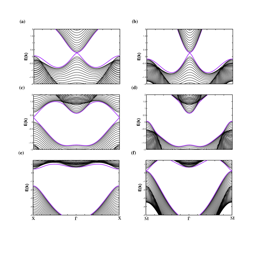
Figure 1: The band dispersion in STKI-I (a)-(b), WTKI (c)-(d), and STKI-II (e)-(f) states along the bond (10) (left panels) and the diagonal (11) (right panels) directions of surface Brillouin zone. The purple curves mark the surface states.

We begin with the electronic structure on the surface of the Kondo insulator. To do so, we have determined the topological characteristics of the Kondo insulating state in the system bulk through the calculation of the $Z_{2}$ topological indices. Dependent on the location of the localized $f$-level $\epsilon_{f}$, the Kondo insulating states can be characterized into two strong topological insulating (STKI) regimes, which are separated by one weak topological insulating (WTKI) regime. MDzero:2010 Hereafter we call the two STKI regimes STKI-I and STKI-II. In previous model calculations, although the topological structure has been systematically studied, no much attention has been paid to the existence of a bulk energy gap near the Fermi energy, which is a necessary condition for a truly insulating bulk. Distinctly, we find that this condition can be satisfied by adjusting the chemical potential self-consistently so that the whole system is close to half filled in our minimal two-orbital model. Thereafter, we present results with the values of bare $f$-level to be $\epsilon_{f}=-17$, $-7.5$, and $2$ to represent the STKI-I, WTKI, and STKI-II regimes. In Fig. 1, the energy dispersion is shown along the in-plane bond and diagonal directions of the surface Brillouin zone (BZ) for the pristine slab geometry. It can be seen that for the WTKI state, there are two Dirac cones located at the $\bar{X}$ points, that is, the edges of the surface BZ. For the STKI-I state, there exists a Dirac cone at the $\bar{\Gamma}$ point, that is, the center of the surface BZ; while for the STKI-II state, there exists a Dirac cone at the $\bar{M}$ points, that is, the corner of the surface BZ. To gain further insight into the structure of the surface metallic states, we show in Fig. 2 the local density of states in the first three surface planes of the slab geometry. Noticeably, the insulating gap for all three regimes is open near the Fermi energy, which makes the notion of Kondo insulator really meaningful. In the STKI-I state, we can see that most of the $f$-electron spectral weight is lumped at the lower edge of the insulating gap, implying a dominant electrons occupation of the $f$-band; while in the STKI-II state, we see that most of the $f$-electron spectral weight is lumped at the upper edge of the insulating gap, implying a minor electron occupation of the $f$-band. In the WTKI state, the $f$-electron spectral weight is about equally distributed at the lower and upper edges of the energy gap. These unique distribution of the $f$-electron spectral weight near the gap edges seems to be closely related to the number of Dirac cones and their locations in the three TKI regimes. Furthermore, one can also see that the dominant peaks in the local density of states at the surface are located closer to the Fermi energy than those deep into the bulk. This band gap narrowing indicates that the Kondo coherence is weakened at the surface as compared to that in the bulk, arising from the disruption of the nearest-neighbor $c$-$f$ hybridization along the direction perpendicular to the surface. The result is also consistent with a recent proposal of surface Kondo breakdown in topological Kondo insulators. OErten:2016

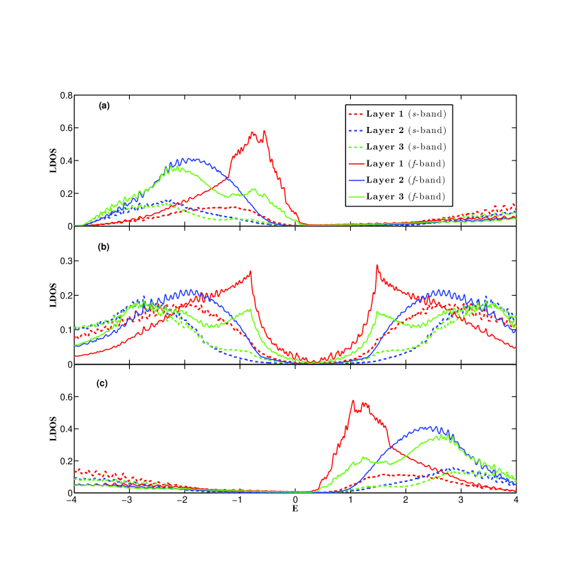
Figure 2: Local density of states near the surface of the Kondo insulator in the STKI-I (a), WTKI (b), and STKI-II (c) regimes. Within each panel, the projected-$s$ and $f$ local density density of states per spin in the first three top layers in a slab structure are shown.

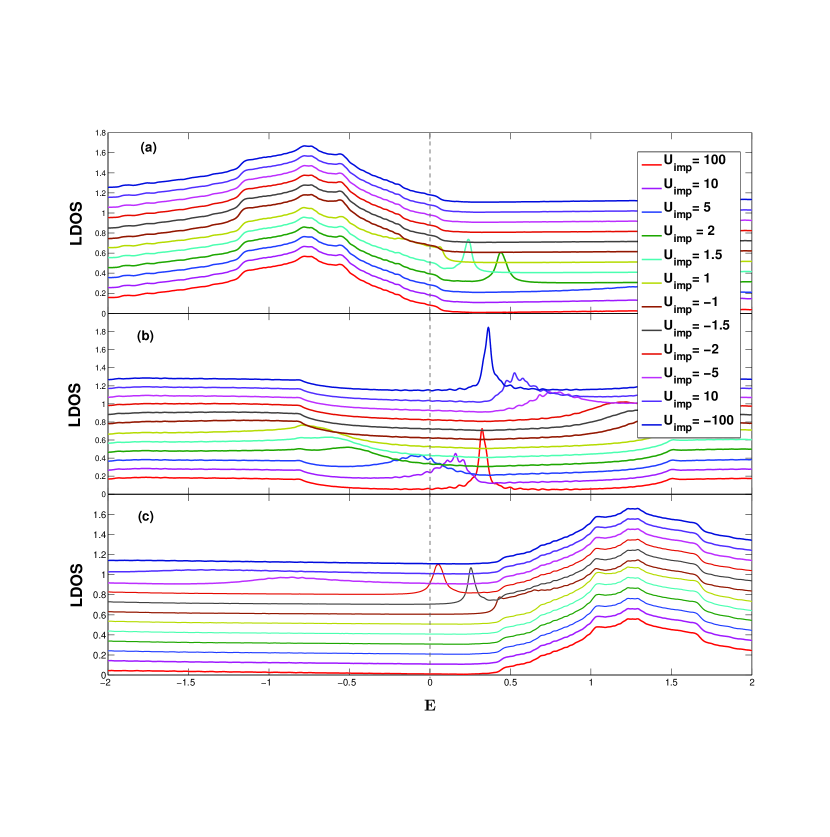
Figure 3: The LDOS for the $f$-electron per spin at a site nearest-neighboring to the single impurity imbedded in on the top layer of the Kondo insulator slab. The bulk states are in the STKI-I (a), WTKI (b), and STKI-II (c) regimes. Within each panel, the LDOS for various values of impurity potential strength is plotted while an offset of 0.1 between two consecutive curves of LDOS is chosen for clarity.

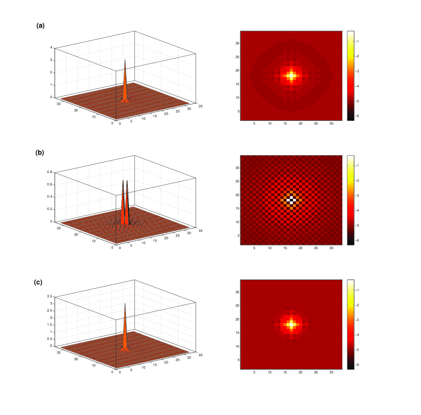
Figure 4: The spatial dependence of the LDOS for the $f$-electron per spin at the resonance energy around a single impurity imbedded at the top layer of the Kondo insulator slab. The left panels are for the surface plots while the right ones are for the image plots with the intensity in log scale. The intra-gap impurity resonance state energy is determined by the strength of the impurity potential in the respective STKI-I (a) [$E_{r}=0.441$ for $U_{\text{imp}}=2.0$], WTKI (b) [$E_{r}=0.324$ for $U_{\text{imp}}=100$], and STKI-II (c) [$E_{r}=0.051$ for $U_{\text{imp}}=-2.0$] regimes.

We next explore the effect of a single impurity on the surface of the Kondo insulator. As we have mentioned in the introduction, a study of the local electronic properties around these single impurities will help elucidate the underlying feature of the electron states. They are especially effective in a wide range of Dirac materials including $d$-wave superconductors, graphene, and surface metallic states in band topological insulators. Figure 3 shows the local density of states (LDOS) around a single nonmagnetic impurity for three regimes of Kondo insulating state. The LDOS is measured at a site nearest neighboring to the impurity site. For each regime, the LDOS for the $f$-electron per spin is shown for a sequence of values of impurity potential strength from the repulsive unitary limit to the attractive unitary limit. For the STKI-I regime, the intragap impurity resonance peak occurs when the strength of the impurity potential is around $U_{\text{imp}}$=2.0, 1.5, and 1.0. Noticeably, the intragap resonance peak is shifted monotonically from positive energy side to the negative energy side and then merges with the spectrum continuum at the lower edge of Kondo insulating gap (see Fig. 3(a)), when the impurity potential is changed from the positive unitary limit toward the negative unitary limit. Correspondingly, for the STKI-II regime, the intragap impurity resonance peak occurs when the strength of the impurity potential is around $U_{\text{imp}}=-2.0$, $-1.5$, and $-1.0$. Now the intragap resonance peak is shifted monotonically from negative energy side to the positive energy side and then merges with the spectrum continuum at the upper edge of Kondo insulating gap (see Fig. 3(c)), when the impurity potential is changed from the negative unitary limit toward the positive unitary limit. Therefore, an interesting dual relation between the STKI-I and STKI-II regimes is established. We emphasize here that in the strong topological Kondo insulating regimes, there exist no impurity resonance states in the unitary limit of impurity scattering. On the contrary, in the WTKI regime, a re-entrant behavior of the impurity resonance state is obtained. The impurity resonance peak is pinned on the lower edge side of the Kondo insulating gap center (see the bottom red line of Fig. 3(b)) in the unitary limit of a repulsive impurity potential. With the decreasing repulsive impurity potential, the peak is shifted toward the negative energy side of the $f$-electron spectrum continuum. After the impurity potential changes sign from being repulsive into being attractive, the resonance peak emerges out of the $f$-electron spectrum continuum with the increased strength of the potential scattering. This peak is finally pinned on the upper edge side of the gap center as the unitary limit of an attractive impurity potential is reached (see the top black line of Fig. 3(b)). Therefore, for the WTKI regime, the most salient feature is that there exist impurity resonance states in the unitary limit of impurity scattering regardless of being repulsive or attractive. The different response of electronic states to the impurity scattering on the surface of different Kondo insulating regimes can also be revealed in the spatial dependence of $f$-electron LDOS around the impurity. As shown in Fig. 4, for the impurity induced resonance states sustained only at the weak scattering of impurity potential in the STKI regimes, the LDOS intensity is spatially peaked at the impurity site itself; while the resonance states sustained at the unitary limit of impurity scattering for the WTKI regime, the LDOS intensity is depressed significantly at the impurity site and exhibits maxima instead at the four sites nearest neighboring (along the bond direction) to the impurity site.

The very different outcome of impurity scattering in the STKI and WTKI regimes, especially the absence of impurity resonance states in the STKI regimes versus the presence of the impurity resonance states in the WTKI regime in the unitary limit of impurity scattering, is believed to be related to the number of the Dirac cones hosted by the surface metallic states, which support only one Dirac cone in the STKI regimes while two Dirac cones in the WTKI regime. On the one hand, our observation for the WTKI regime, with the two Dirac cones on the surface, of the existence of the impurity resonance states in the unitary impurity scattering limit, agrees well with the generic feature of impurity scattering in other types of Dirac materials, where an even number of Dirac cones exist. In particular, we notice that the impurity resonance states have been obtained in the unitary limit of impurity scattering in both two-dimensional $d$-wave superconductors with four Dirac cones and graphene with two Dirac nodes. On the other hand, our observation in the STKI regimes of no impurity resonance states in the unitary impurity scattering limit echoes the expectation that surface metallic states with an odd number of gapless chiral modes supported by a strong topological insulator are enjoying topological protection against surface impurity scattering. Thanks to the stoichiometric nature of the heavy fermion compounds, we expect that the emerging topological Kondo insulators can provide an unprecedented test ground for the rich results uncovered for the surface impurity scattering effect. Although there is no STM study so far to focus on these novel effects from the impurity scattering for the purpose of identifying the topological nature of Kondo insulators, there is equally no reason to exclude such a powerful approach.

IV Concluding remarks

In summary, we have studied the local electronic structure in a Kondo insulator within a minimal-orbital Anderson lattice model. We have shown first that the two strong topological regimes sandwiching the weak topological regime give rise to a single Dirac cone, which is located near the center or corner of the surface Brillouin zone. We have further found that, when a single impurity is placed on the surface, low-energy resonance states are induced in the weak scattering limit for the strong TKI regimes and the resonance level moves monotonically across the hybridization gap with the strength of impurity scattering potential; while low energy states can only be induced in the unitary scattering limit for the weak TKI regime, where the resonance level moves universally toward the center of the hybridization gap. These results on the impurity induced low-energy quasiparticles should be detectable in scanning tunneling microscopy/spectroscopy, which has recently found success in probing into exotic properties in heavy fermion systems.

- (1) M. Z. Hasan and C. L. Kane, Rev. Mod. Phys. 82, 3045 (2010).
- (2) X.-L. Qi and S.-C. Zhang, Phys. Today 63, 33-38 (2010).
- (3) X.-L. Qi and S.-C. Zhang, Rev. Mod. Phys. 83, 1057 (2011).
- (4) T. Xia, , D. Qian, D. Hsieh, L. Wray, A. Pal, H. Lin, A. Bansil, D. Grauer, Y. S. Hor, R. J. Cava, and M. Z. Hasan, Nat. Phys. 5, 398 (2009).
- (5) P. Roushan, J. Seo, C. V. Parker, Y. S. Hor, D. Hsieh, D. Qian, A. Richardella, M. Z. Hasan, R. J. Cava, and A. Yazdani, Nature (London) 460, 1106 (2009).
- (6) T. Zhang, P. Cheng, X. Chen, J. F. Jia, X. C. Ma, K. He, L. L. Wang, H. J. Zhang, X. Dai, Z. Fang, X. C. Xie, and Q. K. Xue, Phys. Rev. Lett. 103, 266803 (2009).
- (7) J. Seo, P. Roushan, H. Beidenkopf, Y. S. Hor, R. J. Cava, and A. Yazdani, Nature (London) 466, 343 (2010).
- (8) Z. Alpichshev, J. G. Analytis, J. H. Chu, I. R. Fisher, Y. L. Chen, Z. X. Shen, A. Fang, and A. Kapitulnik, Phys. Rev. Lett. 104, 016401 (2010).
- (9) B. A. Bernevig, T. L. Hughes, and S. C. Zhang, Science 314, 1757 (2006).
- (10) S. Raghu, X.-L. Qi, C. Honerkamp, and S.-C. Zhang, Phys. Rev. Lett. 100, 156401 (2008).
- (11) K. Sun, H. Yao, E. Fradkin, and S. A. Kivelson, Phys. Rev. Lett. 103, 046811 (2009).
- (12) R. Nandkishore and L. Levitov, Phys. Rev. B 82, 115124 (2010).
- (13) K. Sun, W. V. Liu, A. Hemmerich, and S. Das Sarma, Nat. Phys. 8, 67 (2012).
- (14) H. M. Guo and M. Franz, Phys. Rev. Lett. 103, 206805 (2009).
- (15) D. A. Pesin and L. Balents, Nat. Phys. 6, 376 (2010).
- (16) X. Wan, A. Turner, A. Vishwanath, and S. Y. Savrasov, Phys. Rev. B 83, 205101 (2011).
- (17) B.-J. Yang and Y. B. Kim, Phys. Rev. B 82, 085111 (2010).
- (18) M. Dzero, K. Sun, V. Galitski, and P. Coleman, Phys. Rev. Lett. 104, 106408 (2010).
- (19) X. Zhang, H. Zhang, J. Wang, C. Felser, and S.-C. Zhang, Science 335, 1464 (2012).
- (20) B. Yan, L. Müchler, X.-L. Qi, S. C. Zhang, and C. Felser, Phys. Rev. B 85, 165125 (2012).
- (21) M. Dzero, K. Sun, P. Coleman, and V. Galitski, Phys. Rev. B 85, 045130 (2012).
- (22) M.-T. Tran, T. Takimoto, and K.-S. Kim, Phys. Rev. B 85, 125128 (2012).
- (23) F. Lu, J.-Z. Zhao, H. Weng, Z. Fang, and X. Dai, Phys. Rev. Lett. 110, 096401 (2013).
- (24) X. Deng, K. Haule, and G. Kotliar, Phys. Rev. Lett. 111, 176404 (2013).
- (25) V. Alexandrov, M. Dzero, and P. Coleman, Phys. Rev. Lett. 111, 226403 (2013).
- (26) X.-Y. Feng, J. Dai, C.-H. Chung, and Q. Si, Phys. Rev. Lett. 111, 016402 (2013).
- (27) T. Takimoto, J. Phys. Soc. Jpn. 80, 123710 (2011).
- (28) S. Wolgast, Ç. Kurdak, K. Sun, J. W. Allen, D.-J. Kim, and Fisk, Z. Phys. Rev. B 88, 180405(R) (2013).
- (29) Z. J. Yue, X. L. Wang, D. L. Wang, J. Y. Wang, and S. X. Dou, J. Phys. Soc. Jpn. 84, 044715 (2015).
- (30) G. Li, Z. Xiang, F. Yu, T. Asaba, B. Lawson, P. Cai, C. Tinsman, A. Berkley, S. Wolgast, Y. S. Eo, D.-J. Kim, C. Kurdak, J. W. Allen, K. Sun, X. H. Chen, Y. Y. Wang, Z. Fisk, L. Li, Science 346, 1208 (2014).
- (31) N. Xu, X. Shi, P. K. Biswas, C. E. Matt, R. S. Dhaka, Y. Huang, N. C. Plumb, M. Radović, J. H., Dil, E. Pomjakushina, K. Conder, A. Amato, Z. Salman, D. McK. Paul, J. Mesot, H. Ding, and M. Shi, Phys. Rev. B 88, 121102(R) (2013).
- (32) M. Nupane, N. Alidoust, S.-Y. Xu, T. Kondo, D.-J. Kim, C. Liu, I. Belopolski, T.-R. Chang, H.-T. Jeng, T. Durakiewicz, L. Balicas, H. Lin, A. Bansil, S. Shin, Z. Fisk, and M. Z. Hasan, Nat. Commun. 4, 2991 (2013).
- (33) J. Jiang, S. Li, T. Zhang, Z. Sun, F. Chen, Z. R. Ye, M. Xu, Q. Q. Ge, S. Y. Tan, X. H. Niu, M. Xia, B. P. Xie, Y. F. Li, X. H. Chen, H. H. Wen, and D. L. Feng, Nat. Commun. 4, 3010 (2013).
- (34) M. M. Yee, Y. He, A. Soumyanarayanan, D.-J. Kim, Z. Fisk, and J. E. Hoffman, arxiv.org:1308.1085.
- (35) Z.-H. Zhu, A. Nicolaou, G. Levy, N. P. Butch, P. Syers, X. F. Wang, J. Paglione, G. A. Sawatzky, I. S. Elfimov, and A. Damascelli, Phys. Rev. Lett. 111, 216402 (2013).
- (36) E. Frantzeskakis, N. de Jong, B. Zwartsenberg, Y. K. Huang, Y. Pan, X. Zhang, J. X. Zhang, F. X. Zhang, L. H. Bao, O. Tegus, A. Varykhalov, A. de Visser, and M. S. Golden, Phys. Rev. X 3, 041024 (2013).
- (37) S. Röler, T.-H. Jang, D. J., Kim, L. H. Tjeng, Z. Fisk, F. Steglich, and S. Wirth, Proc. Natl. Acad. Sci. (USA )111, 4798 (2014).
- (38) A. V. Balatsky, I. Vekhter, J.-X. Zhu, Rev. Mod. Phys. 78, 373 (2006).
- (39) J.-X. Zhu, R. Yu, A. V. Balatsky, and Q. Si, Phys. Rev. Lett. 107, 167002 (2011).
- (40) C.-L. Song, and J. E. Hoffman, Curr. Opin. Solid State Mater. Sci. 17, 39 (2013).
- (41) M. H. Hamidian, A. R. Schmidt, I. A. Firmo, M. P. Allan, P. Bradley, J. D. Garrett, T. J. Williams, G. M., Luke, Y. Dubi, A. V. Balatsky, and J. C. Davis, Proc. Natl. Acad. Sci. (USA) 108, 18233 (2011).
- (42) T. Senthil, S. Sachdev, and M. Vojta, Phys. Rev. Lett. 90, 216403 (2003).
- (43) T. Senthil, M. Vojta, and S. Sachdev, Phys. Rev. B 69, 035111 (2004).
- (44) C. Pepin, Phys. Rev. Lett. 98, 206401 (2007).
- (45) J.-X. Zhu, I. Martin, and A. R. Bishop, Phys. Rev. Lett. 100, 236403 (2008).
- (46) P. Gegenwart, Q. Si, and F. Steglich, Nat. Phys. 4, 186 (2008).
- (47) J.-X. Zhu, J.-P. Julien, Y. Dubi, and A. V. Balatsky, Phys. Rev. Lett. 108, 186401 (2012).
- (48) L. Fu, and C. L. Kane, Phys. Rev. B 76, 045302 (2007).
- (49) M. C. Gutzwiller, Phys. Rev. Lett. 10, 159 (1963).
- (50) M. C. Gutzwiller, Phys. Rev. 137, A1726 (1965).
- (51) D. Vollhardt, Rev. Mod. Phys. 56, 99 (1984).
- (52) F. C. Zhang, C. Gross, T. M. Rice, and H. Shiba, Supercond. Sci. Technol. 1, 36 (1988).
- (53) C. Li, S. Zhou, and Z. Wang, Phys. Rev. B 73, 060501(R) (2006).
- (54) J.-P. Julien and J. Bouchet, Prog. Theor. Chem. Phys. 15, 509 (2006).
- (55) Q.-H. Wang, Z. D. Wang, Y. Chen, and F. C. Zhang, Phys. Rev. B 73, 092507 (2006).
- (56) W. H. Ko, C. P. Pave, and P. A. Lee, Phys. Rev. B 76, 245113 (2007).
- (57) N. Fukushima, Phys. Rev. B 78, 115105 (2008).
- (58) Jian-Xin Zhu, Bogoliubov-de Gennes Method and Applictations (Springer, Berlin, 2016).
- (59) O. Erten, P. Ghaemi, and P. Coleman, Phys. Rev. Lett. 116, 046403 (2016).