Asymmetric Clusters and Outliers: Mixtures of Multivariate Contaminated Shifted Asymmetric Laplace Distributions

Abstract

Mixtures of multivariate contaminated shifted asymmetric Laplace distributions are developed for handling asymmetric clusters in the presence of outliers (also referred to as bad points herein). In addition to the parameters of the related non-contaminated mixture, for each (asymmetric) cluster, our model has one parameter controlling the proportion of outliers and one specifying the degree of contamination. Crucially, these parameters do not have to be specified a priori, adding a flexibility to our approach that is absent from other approaches such as trimming. Moreover, each observation is given a posterior probability of belonging to a particular cluster, and of being an outlier or not; advantageously, this allows for the automatic detection of outliers. An expectation-conditional maximization algorithm is outlined for parameter estimation and various implementation issues are discussed. The behaviour of the proposed model is investigated, and compared with well-established finite mixtures, on artificial and real data.

Keywords: Outlier detection, mixture models; model-based clustering; shifted asymmetric Laplace distribution; contaminated normal distribution.

1 Introduction

Clustering algorithms based on probability models are a popular choice for exploring complex data structures. The model-based approach assumes that data are generated by a finite mixture of probability distributions. A $p$-dimensional random vector $\boldsymbol{X}$ is said to arise from a parametric finite mixture of $G$ distributions if its probability density function (pdf) is a convex linear combination of pdfs, i.e.,

$$p\left(\boldsymbol{x}|\boldsymbol{\vartheta}\right)=\sum_{g=1}^{G}\pi_{g}f\left(\boldsymbol{x}|\boldsymbol{\theta}_{g}\right),$$

where $\boldsymbol{\vartheta}=(\pi_{1},\ldots,\pi_{G},\boldsymbol{\theta}_{1},\ldots,\boldsymbol{\theta}_{G})$ is the overall parameter vector, $\pi_{g}\in\left(0,1\right]$ is the mixing proportion, so that $\sum_{g=1}^{G}\pi_{g}=1$, and $f\left(\boldsymbol{x}|\boldsymbol{\theta}_{g}\right)$ is the component pdf, $g=1,\ldots,G$.

In the mixture family, finite mixtures of multivariate normal distributions have received considerable attention because of their computational and theoretical convenience by assuming, in most cases, that each mixture component represents a cluster (or group) within the original data (see, e.g., Fraley and Raftery, 2002 and McNicholas, 2016b). If a component pdf in the mixture is associated with a cluster, as we assume in this paper (see McNicholas, 2016a, Section 9.1), then normal mixture components imply elliptically symmetric (or elliptically contoured) clusters, which is rather restrictive. Other examples of mixtures implying elliptically symmetric clusters are those with multivariate $t$ (Peel and McLachlan, 2000), multivariate power exponential (Zhang and Liang, 2010 and Dang et al., 2015), and multivariate leptokurtic-normal (Bagnato et al., 2017) components. One way to overcome such a restrictiveness is to argue that asymmetric clusters can be approximated quite well by a mixture of several elliptically symmetric densities like the normal one (Dasgupta and Raftery, 1998, McLachlan and Peel, 2000, and Titterington et al., 1985). While this can be very helpful for modelling purposes, it might be misleading when dealing with clustering applications because one group may be represented by more than one component just because it has, in fact, an asymmetric density (see Franczak et al., 2014, for an interesting example). One possible approach to dealing with asymmetric groups consists of considering transformations so as to make the components as elliptical and symmetric as possible, and then fitting mixtures of elliptically symmetric (usually normal) distributions (Schork and Schork, 1988 and Gutierrez et al., 1995). Although such a treatment is very convenient, the achievement of joint elliptical symmetry is rarely satisfied and the transformed variables become more difficult to interpret. Instead of applying transformations, there is a growing interest in proposing mixture models where the component distributions are skewed. Examples in this direction are mixtures of multivariate skew-normal (SN) distributions (Lin, 2009 and Pyne et al., 2009), multivariate shifted asymmetric Laplace (SAL) distributions (Franczak et al., 2014), and other approaches (e.g., Murray et al., 2017a; Tang et al., 2018). The mixture of SAL distributions approach has the advantage to simplify the computational effort required by the EM algorithm to fit the model.

However real data, in addition to being characterized by underlying asymmetric clusters, are often “contaminated” by outliers or otherwise “bad” points. The use of “bad” in this sense is by analogy with Aitkin and Wilson (1980), and refers to points that have a deleterious effect on parameter estimation, including the mixing proportions, as discussed, for example, in Gallegos and Ritter (2009). Thus an important practical application is the development of methods capable of detecting bad points and performing robust parameter estimation when they are present. Examples of mixture models coping with such issues are: mixtures of multivariate skew-$t$ distributions (see, e.g., Wang et al., 2009, Lin, 2010, Lee and McLachlan, 2014, Vrbik and McNicholas, 2012, 2014, and Murray et al., 2014a, 2017b), mixtures of multivariate $t$-distributions with the Box-Cox transformation (Lo and Gottardo, 2012), mixtures of multivariate normal inverse Gaussian distributions (Karlis and Santourian, 2009; Subedi and McNicholas, 2014; O’Hagan et al., 2016), mixtures of multivariate skew-slash distributions (Cabral et al., 2012), mixtures of multivariate generalized hyperbolic distributions (Browne and McNicholas, 2015), scale mixtures of multivariate skew-normal distributions (Basso et al., 2010 and da Silva Ferreira et al., 2011), variance-gamma distributions (McNicholas et al., 2017), hidden truncation hyperbolic distributions (Murray et al., 2017a), and joint generalized hyperbolic distributions (Tang et al., 2018). However, in the methods cited, there is no automatic way of detecting outliers unless one defines some subjective/exogenous trimming rule.

To overcome this drawback, in Section 2 we propose to “contaminate” the components (clusters) of the multivariate SAL mixture to accommodate outliers and to allow for their automatic detection (see Section 4.6). Contamination is introduced by substituting each SAL cluster with a mixture of two SAL pdfs with the same mode and proportional covariance matrices; this is in line with the approach considered by Punzo and McNicholas (2016) to define mixtures of multivariate contaminated normal distributions; see also Maruotti and Punzo (2017) and Mazza and Punzo (2018). According to our contamination scheme, the unimodality of the cluster distribution is preserved (Berger and Berliner, 1986) and its tails are made heavier to accommodate the occurrence of bad points. The choice of working with clusters having a unimodal distribution is justified, but above all natural, if one considers that the most striking feature of a mixture of distributions is often that of multimodality (Bagnato and Punzo, 2013 and Punzo et al., 2018), and a single cluster is most naturally characterized by a unimodal pdf (see McNicholas, 2016a, for further discussion). Indeed, as highlighted in Titterington et al. (1985) and McLachlan and Basford (1988), many papers in applied fields talk not in terms of mixtures but of multimodal distributions; examples are the articles of Murphy (1964) and Brazier et al. (1983) referring to bimodality rather than to mixtures of two distributions.

After a CSAL mixture is fitted on the available data, each observation can be first assigned to one of the clusters, by means of maximum a posteriori probabilities, and then classified as good or bad, and this is a significant advantage, as explained in Section 4.6. Moreover, bad points are automatically down-weighted in the estimation of the parameters of the nested SAL mixture. Thus, we have a model for simultaneous robust clustering, in the presence of asymmetric clusters, and detection of bad points.

Note that the mixture of multivariate skew-contaminated normal (SCN) distributions, introduced by Cabral et al. (2012), is able of coping with skewed clusters under the occurrence of outliers that, eventually, can be also automatically detected (even if the authors do not refer to this possibility). However, although each SCN distribution is defined as a mixture of two SN distributions, the good and bad SN components of this mixture have different modes (see Lachos et al., 2010 and Lachos and Labra, 2014 for details). In this regard note that, although the mode of the SN distribution is unique (Azzalini, 2005 and Azzalini and Capitanio, 2014, p. 126), there is no analytic expression for it (Azzalini and Capitanio, 2014, p. 140). Hence, the SCN mixture cannot be considered as fitting within our contamination scheme.

For maximum likelihood parameter estimation of the CSAL mixture proposed herein, an expectation-conditional maximization (ECM) algorithm (Meng and Rubin, 1993) is developed (Section 3). Further computational and operational aspects are discussed in Section 4. Section 5 investigates the performance of our mixture, in comparison with mixtures of some well-established multivariate elliptically countered and skewed distributions, on artificial and real data. Section 6 provides the conclusion and suggestions for future work. All computational work herein was carried out using R (R Core Team, 2017).

2 Mixtures of contaminated shifted asymmetric Laplace distributions

In this section, we propose to conveniently modify the finite mixture of multivariate shifted asymmetric Laplace (SAL) distributions, proposed by Franczak et al. (2014), for the occurrence of bad points. In situations where clusters may be asymmetric, SAL mixtures, and mixtures of skewed distributions in general, are more appropriate than mixtures of elliptically contoured distributions because they do not overfit the data by including additional components to capture skewness (see, e.g., Lin et al., 2007 and Lin, 2009).

Franczak et al. (2014) give the pdf of a component in a multivariate SAL mixture as

$$f_{\text{SAL}}\left(\boldsymbol{x}|\boldsymbol{\mu},\boldsymbol{\Sigma},\boldsymbol{\alpha}\right)=\frac{2\text{exp}\{\left(\boldsymbol{x}-\boldsymbol{\mu}\right)^{\top}\boldsymbol{\Sigma}^{-1}\boldsymbol{\alpha}\}}{(2\pi)^{p/2}|\boldsymbol{\Sigma}|^{1/2}}\left[\frac{\delta\left(\boldsymbol{x},\boldsymbol{\mu}|\boldsymbol{\Sigma}\right)}{2+\boldsymbol{\alpha}^{\top}\boldsymbol{\Sigma}^{-1}\boldsymbol{\alpha}}\right]^{\nu/2}K_{\nu}(u),$$ (1)

where $\boldsymbol{\mu}$ is the mode (see Dharmadhikari and Joag-Dev, 1988 and Kotz et al., 2012, Chapter 6.6 for details), $\boldsymbol{\Sigma}$ is a scale matrix, $\boldsymbol{\alpha}\in{}^{p}$ denotes the skewness, $\delta\left(\boldsymbol{x},\boldsymbol{\mu}|\boldsymbol{\Sigma}\right)=\left(\boldsymbol{x}-\boldsymbol{\mu}\right)^{\top}\boldsymbol{\Sigma}^{-1}(\boldsymbol{x}-\boldsymbol{\mu})$ is the squared Mahalanobis distance between $\boldsymbol{x}$ and $\boldsymbol{\mu}$, with respect to a scale matrix $\boldsymbol{\Sigma}$, $u=\sqrt{\left(2+\boldsymbol{\alpha}^{\top}\boldsymbol{\Sigma}^{-1}\boldsymbol{\alpha}\right)\delta\left(\boldsymbol{x},\boldsymbol{\mu}|\boldsymbol{\Sigma}\right)}$, and $K_{\nu}$ is the modified Bessel function of the third kind with index $\nu=(2-p)/2$. The mean vector and covariance matrix of the SAL distribution are given by $E\left(\boldsymbol{X}\right)=\boldsymbol{\mu}+\boldsymbol{\alpha}$ and $\text{Cov}\left(\boldsymbol{X}\right)=\boldsymbol{\Sigma}+\boldsymbol{\alpha}\boldsymbol{\alpha}^{\top}$, respectively. Furthermore, Franczak et al. (2014) use the fact that a random vector $\boldsymbol{X}$ whose density is given in (1) can be generated through the relationship

$$\boldsymbol{X}=\boldsymbol{\mu}+W\boldsymbol{\alpha}+\sqrt{W}\boldsymbol{Y},$$ (2)

where $W\sim\mathcal{\text{Exp}}(1)$ and $\boldsymbol{Y}\sim\mathcal{N}_{p}(\boldsymbol{0},\boldsymbol{\Sigma})$, thus $\boldsymbol{X}|W=w\sim\mathcal{N}_{p}\left(\boldsymbol{\mu}+w\boldsymbol{\alpha},w\boldsymbol{\Sigma}\right)$.

To build the framework for model-based clustering with multivariate contaminated SAL mixtures, we follow the approach adopted by Punzo and McNicholas (2016) to define multivariate contaminated normal mixtures. According to this approach, each of the $G$ clusters (components) of the mixture is itself a mixture of two (multivariate normal) components with equal mode and proportional covariance matrices. In each cluster, the component with the lower dispersion fits the good data (“good component”) while the other accommodates the outliers (“bad component”). To apply this idea to the SAL mixture, we employ a contamination scheme where, in each cluster, $\boldsymbol{\Sigma}$ and $\boldsymbol{\alpha}$ of the good SAL component are respectively inflated as $\rho\boldsymbol{\Sigma}$ and $\sqrt{\rho}\boldsymbol{\alpha}$ in the bad SAL component, with $\rho>1$ denoting the contamination factor. This means that, for bad points,

$$\text{Cov}\left(\boldsymbol{X}\right)=\rho\boldsymbol{\Sigma}+\sqrt{\rho}\boldsymbol{\alpha}\sqrt{\rho}\boldsymbol{\alpha}^{\top}=\rho(\boldsymbol{\Sigma}+\boldsymbol{\alpha}\boldsymbol{\alpha}^{\top}),$$

i.e., the covariance matrix for the bad points has been inflated by $\rho$ compared to the covariance matrix for the good points, as in the approach of Punzo and McNicholas (2016). This leads to the contaminated SAL (CSAL) distribution whose pdf is

$$f_{\text{CSAL}}\left(\boldsymbol{x}|\boldsymbol{\mu},\boldsymbol{\Sigma},\boldsymbol{\alpha},\lambda,\rho\right)=\lambda f_{\text{SAL}}\left(\boldsymbol{x}|\boldsymbol{\mu},\boldsymbol{\Sigma},\boldsymbol{\alpha}\right)+\left(1-\lambda\right)f_{\text{SAL}}\left(\boldsymbol{x}|\boldsymbol{\mu},\rho\boldsymbol{\Sigma},\sqrt{\rho}\boldsymbol{\alpha}\right),$$ (3)

where $\lambda\in\left(0,1\right)$ denotes the proportion of good points. The mode and covariance matrix of the bad component $f_{\text{SAL}}\left(\boldsymbol{x}|\boldsymbol{\mu},\rho\boldsymbol{\Sigma},\sqrt{\rho}\boldsymbol{\alpha}\right)$ of the CSAL distribution in (3) are $\boldsymbol{\mu}$ and $\rho(\boldsymbol{\Sigma}+\boldsymbol{\alpha}\boldsymbol{\alpha}^{\top})$, respectively. Hence, the bad component has the same mode $\boldsymbol{\mu}$, and inflated covariance matrix, with respect to the good component; moreover, $\boldsymbol{\mu}$ is also the mode of the CSAL distribution. Thus, our way to contaminate fulfills the requirements of the contamination scheme used by Punzo and McNicholas (2016). We can visualize the result by looking at Figure 1; here, the contours from a bivariate SAL pdf with parameters

$$\boldsymbol{\mu}=\begin{bmatrix}[r]0\\ 0\\ \end{bmatrix},\quad\boldsymbol{\Sigma}=\begin{bmatrix}[r]1&0.5\\ 0.5&1\\ \end{bmatrix}\quad\text{and}\quad\boldsymbol{\alpha}=\begin{bmatrix}[r]1\\ 1\\ \end{bmatrix},$$ (4)

are compared to the contours from a bivariate CSAL pdf with the same parameters $\boldsymbol{\mu}$, $\boldsymbol{\Sigma}$ and $\boldsymbol{\alpha}$ given in (4), with proportion of good observations $\lambda=0.8$ and degree of contamination $\rho=5$.

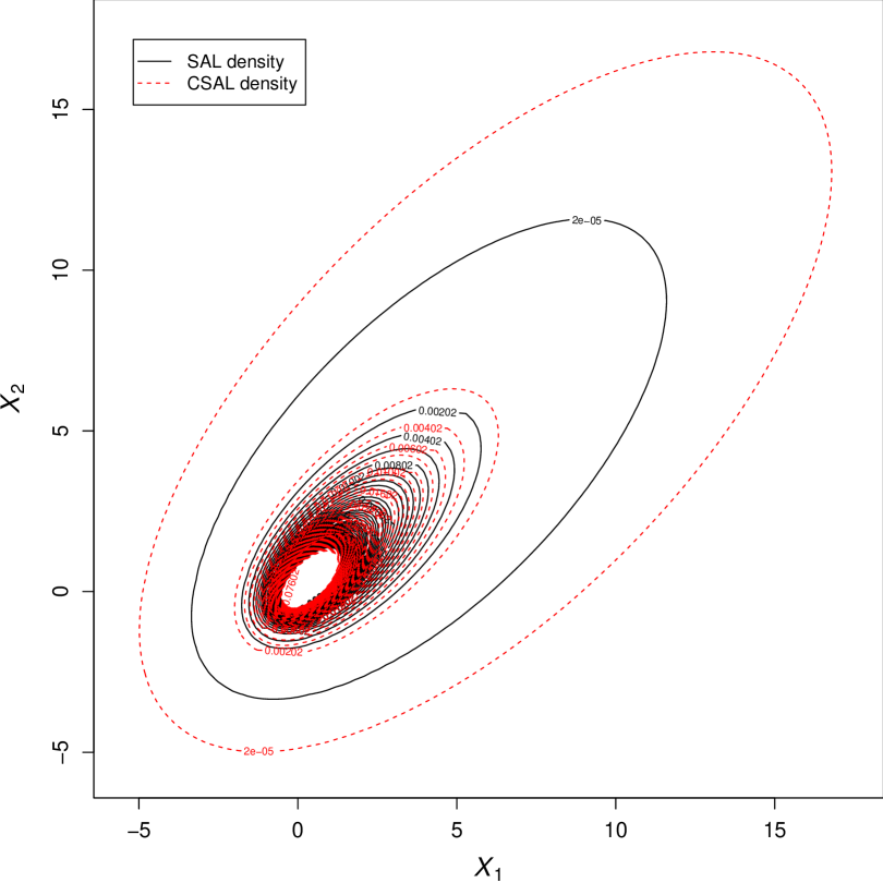
Figure 1: Example of contours comparing the SAL (solid black contours) and CSAL (dashed red contours) distributions.

The assumption of clusters having a CSAL distribution yields the multivariate CSAL mixture with pdf

$$p_{\text{CSAL}}(\boldsymbol{x}|\boldsymbol{\vartheta})=\sum_{g=1}^{G}\pi_{g}\left[\lambda_{g}f_{\text{SAL}}\left(\boldsymbol{x}|\boldsymbol{\mu}_{g},\boldsymbol{\Sigma}_{g},\boldsymbol{\alpha}_{g}\right)+(1-\lambda_{g})f_{\text{SAL}}\left(\boldsymbol{x}|\boldsymbol{\mu}_{g},\rho_{g}\boldsymbol{\Sigma}_{g},\sqrt{\rho_{g}}\boldsymbol{\alpha}_{g}\right)\right],$$ (5)

where $\boldsymbol{\vartheta}=\left(\pi_{1},\ldots,\pi_{G},\boldsymbol{\mu}_{1},\ldots,\boldsymbol{\mu}_{G},\boldsymbol{\Sigma}_{1},\ldots,\boldsymbol{\Sigma}_{G},\boldsymbol{\alpha}_{1},\ldots,\boldsymbol{\alpha}_{G},\lambda_{1},\ldots,\lambda_{G},\rho_{1},\ldots,\rho_{G}\right)$ contains all the parameters of the model.

3 Maximum likelihood estimation: the ECM algorithm

Let $\boldsymbol{x}_{1},\ldots,\boldsymbol{x}_{n}$ be an observed sample from the CSAL mixture model (5). To find maximum likelihood (ML) estimates for the parameters $\boldsymbol{\vartheta}$ of this model, we adopt the expectation-conditional maximization (ECM) algorithm (Meng and Rubin, 1993). The ECM algorithm is a variant of the famous expectation-maximization (EM) algorithm (Dempster et al., 1977). The EM algorithm, as well as its variants, are iterative procedures for finding ML estimates when data are incomplete or are treated as being incomplete. In our case, as in Punzo and McNicholas (2016), there are two hierarchical sources of incompleteness. We have a first-step source of incompleteness, the classical one in the use of mixture models, arising from the fact that for each observation $\boldsymbol{x}_{i}$ we do not know its cluster membership; this source is governed by an indicator vector $\boldsymbol{z}_{i}=\left(z_{i1},\ldots,z_{iG}\right)$, where $z_{ig}=1$ if $\boldsymbol{x}_{i}$ comes from cluster $g$ and $z_{ig}=0$ otherwise. The other source arises from the fact that we do not know whether an observation in group $g$ is good or bad. To denote this second source of missing data, we use the indicator vector $\boldsymbol{v}_{i}=\left(v_{i1},\ldots,v_{iG}\right)$ so that $v_{ig}=1$ if ${\boldsymbol{x}}_{i}$ in group $g$ is good and $v_{ig}=0$ if $\boldsymbol{x}_{i}$ in group $g$ is bad. The values of $z_{ig}$ and $v_{ig}$ are used for the definition of the following complete-data likelihood

$$L_{c}\left(\boldsymbol{\vartheta}\right)=\prod_{i=1}^{n}\prod_{g=1}^{G}\Big{\{}\pi_{g}[\lambda_{g}f_{\text{SAL}}(\boldsymbol{x}_{i}|\boldsymbol{\mu}_{g},\boldsymbol{\Sigma}_{g},\boldsymbol{\alpha}_{g})]^{v_{ig}}[(1-\lambda_{g})f_{\text{SAL}}(\boldsymbol{x}_{i}|\boldsymbol{\mu}_{g},\rho_{g}\boldsymbol{\Sigma}_{g},\sqrt{\rho_{g}}\boldsymbol{\alpha}_{g})]^{(1-v_{ig})}\Big{\}}^{z_{ig}}.$$ (6)

The complete-data log-likelihood corresponding to (6) can be written as

$$l_{c}\left(\boldsymbol{\vartheta}\right)=l_{c1}\left(\boldsymbol{\pi}\right)+l_{c2}\left(\boldsymbol{\lambda}\right)+l_{c3}^{\text{good}}\left(\boldsymbol{\mu},\boldsymbol{\Sigma},\boldsymbol{\alpha}\right)+l_{c3}^{\text{bad}}\left(\boldsymbol{\mu},\boldsymbol{\Sigma},\boldsymbol{\alpha},\boldsymbol{\rho}\right),$$ (7)

where

$$l_{c1}\left(\boldsymbol{\pi}\right)=\sum_{i=1}^{n}\sum_{g=1}^{G}{z}_{ig}\ln\pi_{g},$$

$$l_{c2}\left(\boldsymbol{\lambda}\right)=\sum_{i=1}^{n}\sum_{g=1}^{G}z_{ig}\left[v_{ig}\ln\lambda_{g}+\left(1-v_{ig}\right)\ln\left(1-\lambda_{g}\right)\right],$$

$$l_{c3}^{\text{good}}\left(\boldsymbol{\mu},\boldsymbol{\Sigma},\boldsymbol{\alpha}\right)=\sum_{i=1}^{n}\sum_{g=1}^{G}z_{ig}v_{ig}\log\left[f_{\text{SAL}}(\boldsymbol{x}_{i}|\boldsymbol{\mu}_{g},\boldsymbol{\Sigma}_{g},\boldsymbol{\alpha}_{g})\right]$$

and

$$l_{c3}^{\text{bad}}\left(\boldsymbol{\mu},\boldsymbol{\Sigma},\boldsymbol{\alpha},\boldsymbol{\rho}\right)=\sum_{i=1}^{n}\sum_{g=1}^{G}z_{ig}\left(1-v_{ig}\right)\log\left[f_{\text{SAL}}(\boldsymbol{x}_{i}|\boldsymbol{\mu}_{g},\rho_{g}\boldsymbol{\Sigma}_{g},\sqrt{\rho_{g}}\boldsymbol{\alpha}_{g})\right],$$

with $\boldsymbol{\pi}=\left(\pi_{1},\ldots,\pi_{G}\right)$, $\boldsymbol{\lambda}=\left(\lambda_{1},\ldots,\lambda_{G}\right)$, $\boldsymbol{\mu}=\left(\boldsymbol{\mu}_{1},\ldots,\boldsymbol{\mu}_{G}\right)$, $\boldsymbol{\Sigma}=\left(\boldsymbol{\Sigma}_{1},\ldots,\boldsymbol{\Sigma}_{G}\right)$, $\boldsymbol{\alpha}=\left(\boldsymbol{\alpha}_{1},\ldots,\boldsymbol{\alpha}_{G}\right)$ and $\boldsymbol{\rho}=\left(\rho_{1},\ldots,\rho_{G}\right)$. Computationally, it is more efficient to use the relationship between the SAL and normal distributions outlined in (2) to rewrite $l_{c3}^{\text{good}}$ and $l_{c3}^{\text{bad}}$ as

$$l_{c3}^{\text{good}}\left(\boldsymbol{\mu},\boldsymbol{\Sigma},\boldsymbol{\alpha}\right)=\sum_{i=1}^{n}\sum_{g=1}^{G}z_{ig}v_{ig}\log\left[f_{\text{N}}(\boldsymbol{x}_{i}|\boldsymbol{\mu}_{g}+w_{ig}\boldsymbol{\alpha}_{g},w_{ig}\boldsymbol{\Sigma}_{g})f_{\text{Exp}}(w_{ig}|1)\right]$$

and

$$l_{c3}^{\text{bad}}\left(\boldsymbol{\mu},\boldsymbol{\Sigma},\boldsymbol{\alpha},\boldsymbol{\rho}\right)=\sum_{i=1}^{n}\sum_{g=1}^{G}z_{ig}(1-v_{ig})\log\left[f_{\text{N}}(\boldsymbol{x}_{i}|\boldsymbol{\mu}_{g}+w_{ig}\sqrt{\rho_{g}}\boldsymbol{\alpha}_{g},w_{ig}\rho_{g}\boldsymbol{\Sigma}_{g})f_{\text{Exp}}(w_{ig}|1)\right],$$

where $f_{\text{Exp}}\left(\cdot|1\right)$ denotes the pdf of an exponential distribution with rate 1, i.e., $f_{\text{Exp}}\left(w_{ig}|1\right)=e^{-w_{ig}}$, $w_{ig}>0$.

The ECM algorithm iterates between three steps, one E-step and two CM-steps, until convergence. The only difference from the EM algorithm is that each M-step is replaced by two simpler CM-steps. They arise from the partition $\boldsymbol{\vartheta}=\left(\boldsymbol{\vartheta}_{1},\boldsymbol{\vartheta}_{2}\right)$, where $\boldsymbol{\vartheta}_{1}=\left(\boldsymbol{\pi},\boldsymbol{\mu},\boldsymbol{\Sigma},\boldsymbol{\alpha},\boldsymbol{\lambda}\right)$ and $\boldsymbol{\vartheta}_{2}=\boldsymbol{\rho}$. The three steps of the ECM algorithm, for the generic $\left(r+1\right)$th iteration, $r=1,2,\ldots$, are detailed below.

3.1 E-step

The E-step requires the calculation of $Q\left(\boldsymbol{\vartheta}\right)=E[l_{c}\left(\boldsymbol{\vartheta}\right)|\boldsymbol{x}_{1},\ldots,\boldsymbol{x}_{n},\boldsymbol{\vartheta}^{(r)}]$, the conditional expectation of $l_{c}\left(\boldsymbol{\vartheta}\right)$ given the observed data $\boldsymbol{x}_{1},\ldots,\boldsymbol{x}_{n}$, using the current fit $\boldsymbol{\vartheta}^{(r)}$ for $\boldsymbol{\vartheta}$. According to the decomposition of $l_{c}\left(\boldsymbol{\vartheta}\right)$ in (7), the $Q$ function can be written as

$$Q\left(\boldsymbol{\vartheta}\right)=Q_{1}\left(\boldsymbol{\pi}\right)+Q_{2}\left(\boldsymbol{\lambda}\right)+Q_{3}^{\text{good}}\left(\boldsymbol{\mu},\boldsymbol{\Sigma},\boldsymbol{\alpha}\right)+Q_{3}^{\text{bad}}\left(\boldsymbol{\mu},\boldsymbol{\Sigma},\boldsymbol{\alpha},\boldsymbol{\rho}\right),$$

where

$$Q_{1}\left(\boldsymbol{\pi}\right)=\sum_{g=1}^{G}n_{g}^{(r)}\ln\pi_{g},$$ (8)

$$Q_{2}\left(\boldsymbol{\lambda}\right)=\sum_{i=1}^{n}\sum_{g=1}^{G}z_{ig}^{(r)}\left[v_{ig}^{(r)}\ln\lambda_{g}+\left(1-v_{ig}^{(r)}\right)\ln\left(1-\lambda_{g}\right)\right],$$ (9)

$$Q_{3}^{\text{good}}\left(\boldsymbol{\mu},\boldsymbol{\Sigma},\boldsymbol{\alpha}\right)= -\frac{np}{2}\ln\left(2\pi\right)-\frac{1}{2}\sum_{g=1}^{G}n_{g,\text{good}}^{(r)}\ln\left|\boldsymbol{\Sigma}_{g}\right|-\frac{p}{2}\sum_{i=1}^{n}\sum_{g=1}^{G}z_{ig}^{(r)}v_{ig}^{(r)}E_{3ig}^{(r)}$$

$$-\frac{1}{2}\sum_{i=1}^{n}\sum_{g=1}^{G}z_{ig}^{(r)}v_{ig}^{(r)}E_{2ig}^{(r)}\left(\boldsymbol{x}_{i}-\boldsymbol{\mu}_{g}\right)^{\top}\boldsymbol{\Sigma}_{g}^{-1}\left(\boldsymbol{x}_{i}-\boldsymbol{\mu}_{g}\right)+\sum_{i=1}^{n}\sum_{g=1}^{G}z_{ig}^{(r)}v_{ig}^{(r)}\left(\boldsymbol{x}_{i}-\boldsymbol{\mu}_{g}\right)^{\top}\boldsymbol{\Sigma}_{g}^{-1}\boldsymbol{\alpha}_{g}$$

$$-\frac{1}{2}\sum_{i=1}^{n}\sum_{g=1}^{G}z_{ig}^{(r)}v_{ig}^{(r)}E_{1ig}^{(r)}\boldsymbol{\alpha}_{g}^{\top}\boldsymbol{\Sigma}_{g}^{-1}\boldsymbol{\alpha}_{g}-\sum_{i=1}^{n}\sum_{g=1}^{G}z_{ig}^{(r)}v_{ig}^{(r)}E_{1ig}^{(r)}$$ (10)

and

$$Q_{4}^{\text{bad}}\left(\boldsymbol{\mu},\boldsymbol{\Sigma},\boldsymbol{\alpha},\boldsymbol{\rho}\right)= -\frac{np}{2}\ln\left(2\pi\right)-\frac{1}{2}\sum_{g=1}^{G}n_{g,\text{bad}}^{(r)}\ln\left|\boldsymbol{\Sigma}_{g}\right|-\frac{p}{2}\sum_{g=1}^{G}n_{g,\text{bad}}^{(r)}\ln\rho_{g}-\frac{p}{2}\sum_{i=1}^{n}\sum_{g=1}^{G}z_{ig}^{(r)}\left(1-v_{ig}^{(r)}\right)\widetilde{E}_{3ig}^{(r)}$$

$$-\frac{1}{2}\sum_{i=1}^{n}\sum_{g=1}^{G}z_{ig}^{(r)}\left(1-v_{ig}^{(r)}\right)\widetilde{E}_{2ig}^{(r)}\frac{1}{\rho_{g}}\left(\boldsymbol{x}_{i}-\boldsymbol{\mu}_{g}\right)^{\top}\boldsymbol{\Sigma}_{g}^{-1}\left(\boldsymbol{x}_{i}-\boldsymbol{\mu}_{g}\right)$$

$$+\sum_{i=1}^{n}\sum_{g=1}^{G}z_{ig}^{(r)}\left(1-v_{ig}^{(r)}\right)\frac{1}{\sqrt{\rho_{g}}}\left(\boldsymbol{x}_{i}-\boldsymbol{\mu}_{g}\right)^{\top}\boldsymbol{\Sigma}_{g}^{-1}\boldsymbol{\alpha}_{g}$$

$$-\frac{1}{2}\sum_{i=1}^{n}\sum_{g=1}^{G}z_{ig}^{(r)}\left(1-v_{ig}^{(r)}\right)\widetilde{E}_{1ig}^{(r)}\sqrt{\rho_{g}}\boldsymbol{\alpha}_{g}^{\top}\boldsymbol{\Sigma}_{g}^{-1}\boldsymbol{\alpha}_{g}-\sum_{i=1}^{n}\sum_{g=1}^{G}z_{ig}^{(r)}\left(1-v_{ig}^{(r)}\right)\widetilde{E}_{1ig}^{(r)},$$ (11)

with $n_{g}^{(r)}=\sum_{i=1}^{n}z_{ig}^{(r)}$ being the expected size of group $g$, $n_{g,\text{good}}^{(r)}=\sum_{i=1}^{n}z_{ig}^{(r)}v_{ig}^{(r)}$ the expected number of good observations in group $g$, and $n_{g,\text{bad}}^{(r)}=\sum_{i=1}^{n}z_{ig}^{(r)}(1-v_{ig}^{(r)})$ the expected number of bad observations in group $g$. Inside the formulae (8)–(11) there are the following updates

$$z_{ig}^{(r)}\colonequals E\left(Z_{ig}=1|\boldsymbol{x}_{i},\boldsymbol{\vartheta}^{(r)}\right)=\frac{\pi_{g}^{(r)}f_{\text{CSAL}}\left(\boldsymbol{x}_{i}|\boldsymbol{\mu}_{g}^{(r)},\boldsymbol{\Sigma}_{g}^{(r)},\boldsymbol{\alpha}_{g}^{(r)},\lambda_{g}^{(r)},\rho_{g}^{(r)}\right)}{\displaystyle\sum_{h=1}^{G}\pi_{h}f_{\text{CSAL}}\left(\boldsymbol{x}_{i}|\boldsymbol{\mu}_{h}^{(r)},\boldsymbol{\Sigma}_{h}^{(r)},\boldsymbol{\alpha}_{h}^{(r)},\lambda_{h}^{(r)},\rho_{h}^{(r)}\right)},$$

$$v_{ig}^{(r)}\colonequals E\left(V_{ig}=1|\boldsymbol{x}_{i},Z_{ig}=1,\boldsymbol{\vartheta}^{(r)}\right)=\frac{\lambda_{g}^{(r)}f_{\text{SAL}}\left(\boldsymbol{x}_{i}|\boldsymbol{\mu}_{g}^{(r)},\boldsymbol{\Sigma}_{g}^{(r)},\boldsymbol{\alpha}_{g}^{(r)}\right)}{f_{\text{CSAL}}\left(\boldsymbol{x}_{i}|\boldsymbol{\mu}_{g}^{(r)},\boldsymbol{\Sigma}_{g}^{(r)},\boldsymbol{\alpha}_{g}^{(r)},\lambda_{g}^{(r)},\rho_{g}^{(r)}\right)},$$

$$E_{1ig}^{(r)}\colonequals E\left(W_{ig}|\boldsymbol{x}_{i},Z_{ig}=1,\boldsymbol{\vartheta}^{(r)}\right)=\frac{\sqrt{b_{ig}^{(r)}}K_{\nu+1}\left(\sqrt{a_{g}^{(r)}b_{ig}^{(r)}}\right)}{\sqrt{a_{g}^{(r)}}K_{\nu}\left(\sqrt{a_{g}^{(r)}b_{ig}^{(r)}}\right)},$$ (12)

$$E_{2ig}^{(r)}\colonequals E\left(W_{ig}^{-1}|\boldsymbol{x}_{i},Z_{ig}=1,\boldsymbol{\vartheta}^{(r)}\right)=\frac{\sqrt{a_{g}^{(r)}}K_{\nu+1}\left(\sqrt{a_{g}^{(r)}b_{ig}^{(r)}}\right)}{\sqrt{b_{ig}^{(r)}}K_{\nu}\left(\sqrt{a_{g}^{(r)}b_{ig}^{(r)}}\right)}-\frac{2\nu}{b_{ig}^{(r)}},$$ (13)

$$E_{3ig}^{(r)}\colonequals E\left(\ln W_{ig}|\boldsymbol{x}_{i},Z_{ig}=1,\boldsymbol{\vartheta}^{(r)}\right)=\ln\frac{\sqrt{b_{ig}^{(r)}}}{\sqrt{a_{g}^{(r)}}}+\frac{\partial}{\partial\nu}\ln K_{\nu}\left(\sqrt{a_{g}^{(r)}b_{ig}^{(r)}}\right),$$ (14)

$$\widetilde{E}_{1ig}^{(r)}\colonequals E\left(\widetilde{W}_{ig}|\boldsymbol{x}_{i},Z_{ig}=1,\boldsymbol{\vartheta}^{(r)}\right)=\frac{\sqrt{\widetilde{b}_{ig}^{(r)}}K_{\nu+1}\left(\sqrt{a_{g}^{(r)}\widetilde{b}_{ig}^{(r)}}\right)}{\sqrt{a_{g}^{(r)}}K_{\nu}\left(\sqrt{a_{g}^{(r)}\widetilde{b}_{ig}^{(r)}}\right)},$$ (15)

$$\widetilde{E}_{2ig}^{(r)}\colonequals E\left(\widetilde{W}_{ig}^{-1}|\boldsymbol{x}_{i},Z_{ig}=1,\boldsymbol{\vartheta}^{(r)}\right)=\frac{\sqrt{a_{g}^{(r)}}K_{\nu+1}\left(\sqrt{a_{g}^{(r)}\widetilde{b}_{ig}^{(r)}}\right)}{\sqrt{\widetilde{b}_{ig}^{(r)}}K_{\nu}\left(\sqrt{a_{g}^{(r)}\widetilde{b}_{ig}^{(r)}}\right)}-\frac{2\nu}{\widetilde{b}_{ig}^{(r)}},$$ (16)

and

$$\widetilde{E}_{3ig}^{(r)}\colonequals E\left(\ln\widetilde{W}_{ig}|\boldsymbol{x}_{i},Z_{ig}=1,\boldsymbol{\vartheta}^{(r)}\right)=\ln\frac{\sqrt{\widetilde{b}_{ig}^{(r)}}}{\sqrt{a_{g}^{(r)}}}+\frac{\partial}{\partial\nu}\ln K_{\nu}\left(\sqrt{a_{g}^{(r)}\widetilde{b}_{ig}^{(r)}}\right)$$ (17)

where $a_{g}^{(r)}=2+(\boldsymbol{\alpha}_{g}^{(r)})^{\top}(\boldsymbol{\Sigma}_{g}^{(r)})^{-1}\boldsymbol{\alpha}_{g}^{(r)}$, $b_{ig}^{(r)}=\delta(\boldsymbol{x}_{i},\boldsymbol{\mu}_{g}^{(r)}|\boldsymbol{\Sigma}_{g}^{(r)})$, $\widetilde{b}_{ig}^{(r)}=\delta(\boldsymbol{x}_{i},\boldsymbol{\mu}_{g}^{(r)}|\rho_{g}^{(r)}\boldsymbol{\Sigma}_{g}^{(r)})$ and $\nu=(2-p)/2$. The closed forms for $E_{1ig}^{(r)}$, $E_{2ig}^{(r)}$, $E_{3ig}^{(r)}$, $\widetilde{E}_{1ig}^{(r)}$, $\widetilde{E}_{2ig}^{(r)}$ and $\widetilde{E}_{3ig}^{(r)}$ in (12)–(17) exist because $W_{ig}|\boldsymbol{x}_{1},Z_{ig}=1\sim\mathcal{GIG}(a_{g},b_{ig},(2-p)/2)$ and $\widetilde{W}_{ig}|\boldsymbol{x}_{1},Z_{ig}=1\sim\mathcal{GIG}(a_{g},\widetilde{b}_{ig},(2-p)/2)$, where $\mathcal{GIG}\left(a,b,\nu\right)$ denotes the generalized inverse Gaussian (GIG) distribution with parameters $a>0$, $b>0$ and $\nu\in\real$. Note that the terms of the Q-function where $E_{3ig}^{(r)}$ and $\widetilde{E}_{3ig}^{(r)}$ appear — refer to (10) and (11) — are constant with respect to the model parameters $\boldsymbol{\vartheta}$; therefore, $E_{3ig}^{(r)}$ and $\widetilde{E}_{3ig}^{(r)}$ are not required in our calculations but we provide them for completeness.

3.2 CM-step 1

The first CM-step requires the calculation of $\boldsymbol{\vartheta}_{1}^{\left(r+1\right)}$ as the value of $\boldsymbol{\vartheta}_{1}$ that maximizes $Q(\boldsymbol{\vartheta})$ with $\boldsymbol{\vartheta}_{2}$ fixed at $\boldsymbol{\vartheta}_{2}^{(r)}$. In particular, the maximization of $Q_{1}(\boldsymbol{\pi})$ with respect to $\boldsymbol{\pi}$, subject to the constraints on these parameters, yields

$$\pi_{g}^{(r+1)}=\frac{n_{g}^{(r)}}{n},\quad g=1,\ldots,G.$$

Analogously, the maximization of $Q_{2}(\boldsymbol{\lambda})$ with respect to the generic element $\lambda_{g}$ of $\boldsymbol{\lambda}$, $g=1,\ldots,G$, leads to

$$\lambda_{g}^{(r+1)}=\frac{n_{g,\text{good}}^{(r)}}{n_{g}^{(r)}}.$$

Finally, the maximization of $Q_{3}^{\text{good}}(\boldsymbol{\mu},\boldsymbol{\Sigma},\boldsymbol{\alpha})$ and $Q_{3}^{\text{bad}}(\boldsymbol{\mu},\boldsymbol{\Sigma},\boldsymbol{\alpha},\boldsymbol{\rho})$, with respect to the $g$th elements of $\boldsymbol{\mu}$, $\boldsymbol{\Sigma}$ and $\boldsymbol{\alpha}$, $g=1,\ldots,G$, yields

$$\boldsymbol{\mu}_{g}^{(r+1)}=\frac{B^{(r)}\left[\displaystyle\sum_{i=1}^{n}z_{ig}^{(r)}\left(v_{ig}^{(r)}E_{2ig}^{(r)}+\frac{1-v_{ig}^{(r)}}{\rho_{g}^{(r)}}\widetilde{E}_{2ig}^{(r)}\right)\boldsymbol{x}_{i}\right]-C^{(r)}\left[\displaystyle\sum_{i=1}^{n}z_{ig}^{(r)}\left(v_{ig}^{(r)}+\frac{1-v_{ig}^{(r)}}{\rho_{g}^{(r)}}\right)\boldsymbol{x}_{i}\right]}{B^{(r)}A^{(r)}-\left(C^{(r)}\right)^{2}},$$

$$\boldsymbol{\alpha}_{g}^{(r+1)}=\frac{A^{(r)}\left[\displaystyle\sum_{i=1}^{n}z_{ig}^{(r)}\left(v_{ig}^{(r)}+\frac{1-v_{ig}^{(r)}}{\sqrt{\rho_{g}^{(r)}}}\right)\boldsymbol{x}_{i}\right]-D^{(r)}\left[\displaystyle\sum_{i=1}^{n}z_{ig}^{(r)}\left(v_{ig}^{(r)}E_{2ig}^{(r)}+\frac{1-v_{ig}^{(r)}}{\rho_{g}^{(r)}}\widetilde{E}_{2ig}^{(r)}\right)\boldsymbol{x}_{i}\right]}{B^{(r)}A^{(r)}-\left(D^{(r)}\right)^{2}},$$

and

$$\boldsymbol{\Sigma}_{g}^{(r+1)}= \frac{1}{n_{g}^{(r)}}\sum_{i=1}^{n}z_{ig}^{(r)}\left(v_{ig}^{(r)}E_{2ig}^{(r)}+\frac{1-v_{ig}^{(r)}}{\rho_{g}^{(r)}}\widetilde{E}_{2ig}^{(r)}\right)\left(\boldsymbol{x}_{i}-\boldsymbol{\mu}_{g}^{(r+1)}\right)\left(\boldsymbol{x}_{i}-\boldsymbol{\mu}_{g}^{(r+1)}\right)^{\top}$$

$$-\frac{2}{n_{g}^{(r)}}\sum_{i=1}^{n}z_{ig}^{(r)}\left(v_{ig}^{(r)}+\frac{1-v_{ig}^{(r)}}{\sqrt{\rho_{g}^{(r)}}}\right)\left(\boldsymbol{x}_{i}-\boldsymbol{\mu}_{g}^{(r+1)}\right)\left(\boldsymbol{\alpha}_{g}^{(r+1)}\right)^{\top}$$

$$+\frac{1}{n_{g}^{(r)}}\sum_{i=1}^{n}z_{ig}^{(r)}\left[v_{ig}^{(r)}E_{1ig}^{(r)}+\left(1-v_{ig}^{(r)}\right)\widetilde{E}_{1ig}^{(r)}\right]\boldsymbol{\alpha}_{g}^{(r+1)}\left(\boldsymbol{\alpha}_{g}^{(r+1)}\right)^{\top},$$

where

$$A^{(r)}=\sum_{i=1}^{n}z_{ig}^{(r)}\left(v_{ig}^{(r)}E_{2ig}^{(r)}+\frac{1-v_{ig}^{(r)}}{\rho_{g}^{(r)}}\widetilde{E}_{2ig}^{(r)}\right),$$

$$B^{(r)}=\sum_{i=1}^{n}z_{ig}^{(r)}\left[v_{ig}^{(r)}E_{1ig}^{(r)}+\left(1-v_{ig}^{(r)}\right)\widetilde{E}_{1ig}^{(r)}\right],$$

$$C^{(r)}=\sum_{i=1}^{n}z_{ig}^{(r)}\left(v_{ig}^{(r)}+\frac{1-v_{ig}^{(r)}}{\rho_{g}^{(r)}}\right),$$

and

$$D^{(r)}=\sum_{i=1}^{n}z_{ig}^{(r)}\left(v_{ig}^{(r)}+\frac{1-v_{ig}^{(r)}}{\sqrt{\rho_{g}^{(r)}}}\right).$$

3.3 CM-step 2

The second CM-step requires the calculation of $\boldsymbol{\vartheta}_{2}^{\left(r+1\right)}$ as the value of $\boldsymbol{\vartheta}_{2}$ that maximizes $Q(\boldsymbol{\vartheta})$ with $\boldsymbol{\vartheta}_{1}$ fixed at $\boldsymbol{\vartheta}_{1}^{\left(r+1\right)}$. In particular, we have to maximize $Q_{4}^{\text{bad}}\left(\boldsymbol{\mu}=\boldsymbol{\mu}^{(r+1)},\boldsymbol{\Sigma}=\boldsymbol{\Sigma}^{(r+1)},\boldsymbol{\alpha}=\boldsymbol{\alpha}^{(r+1)},\boldsymbol{\rho}\right)$ with respect to each element $\rho_{g}$ of $\boldsymbol{\rho}$, $g=1,\ldots,G$, under the constraint $\rho_{g}>1$. Operationally, the optimize() function, in the stats package for R, can be used to perform a numerical search of the maximum.

4 Further computational and operational aspects

4.1 Initialization strategy

The choice of the initialization strategy for EM-based algorithms constitutes an important issue (see, e.g., Biernacki et al., 2003 and Karlis and Xekalaki, 2003). For the ECM algorithm described in Section 3, we adopt an initialization strategy arising by the fact that the $G$-component SAL mixture can be seen as a special case of the $G$-component CSAL mixture when $\lambda_{g}\rightarrow 1$ and $\rho_{g}\rightarrow 1$, $g=1,\ldots,G$ (nested models). Specifically, we initialize the EM algorithm to fit the $G$-component SAL mixture (see Franczak et al., 2014, for details) by providing the initial indicator vectors $\boldsymbol{z}_{1}^{(0)},\ldots,\boldsymbol{z}_{n}^{(0)}$ for the first M-step; we obtain these vectors by a preliminary run of the $k$-means method (as implemented by the kmeans() function of the stats package for R). The obtained estimates of $\pi_{1},\ldots,\pi_{G}$, $\boldsymbol{\mu}_{1},\ldots,\boldsymbol{\mu}_{G}$, $\boldsymbol{\Sigma}_{1},\ldots,\boldsymbol{\Sigma}_{G}$, and $\boldsymbol{\alpha}_{1},\ldots,\boldsymbol{\alpha}_{G}$ for the SAL mixture, along with the values $\lambda_{1}=\cdots=\lambda_{G}=0.999$ and $\rho_{1}=\cdots=\rho_{G}=1.001$, are used to initialize the first E-step of the ECM algorithm to fit the $G$-component CSAL mixture. From an operational point of view, such an initialization strategy, thanks to the monotonicity property of the ECM algorithm (see, e.g., McLachlan and Krishnan, 2007, p. 28), guarantees that the observed-data log-likelihood of the CSAL mixture will be always greater than, or equal to, the observed-data log-likelihood of the SAL mixture. See Punzo and McNicholas (2016, 2017) and Mazza and Punzo (2018) for an analogous initialization strategy applied to mixtures based on the contaminated normal distribution.

4.2 Convergence criterion

We use a stopping criterion based on the Aitken acceleration (Aitken, 1926) to determine convergence of the ECM algorithm illustrated in Section 3. The commonly used stopping rules can yield convergence earlier than the Aitken stopping criterion, resulting in estimates that might not be close to the ML estimates. The Aitken acceleration at iteration $r$ is

$$a^{\left(r\right)}=\frac{l^{\text{new}}-l^{\left(r\right)}}{l^{\left(r\right)}-l^{\left(r-1\right)}},$$

where $l^{\left(r\right)}$ is the (observed-data) log-likelihood from iteration $r$. An asymptotic — with respect to the iteration number — estimate of the log-likelihood at iteration $r+1$ can be computed via

$$l_{A}^{\text{new}}=l^{\left(q\right)}+\frac{1}{1-a^{\left(r\right)}}\left(l^{\text{new}}-l^{\left(r\right)}\right),$$

see Böhning et al. (1994). Convergence is assumed to have been reached when $l_{A}^{\text{new}}-l^{\left(r\right)}<\epsilon$, provided that this difference is positive (see McNicholas et al., 2010). We use $\epsilon=10^{-15}$ in the analyses of Section 5.

4.3 Dealing with infinite log-likelihood values

As well-documented in Franczak et al. (2014, Section 3.4.2) in the case of the SAL mixture, complications may arise when updating the component mean vectors if $\boldsymbol{\mu}_{g}^{(r)}$, $g=1,\ldots,G$, tends to an observation $\boldsymbol{x}_{i}$. In such situations, computational issues arise when we try to determine the remaining parameter values and, specifically, the expected values $E_{2ig}^{(r)}$ and $\widetilde{E}_{2ig}^{(r)}$. To overcome this problem, we stop updating $\boldsymbol{\mu}_{g}$ when its value equals some $\boldsymbol{x}_{i}$. Details about how to implement this simple-minded procedure can be found in Franczak et al. (2014, Section 3.4.2).

4.4 Model selection

In model-based clustering applications, it is common to fit a mixture model for a range of values of the number of components $G$. After that, the “best” value for $G$ is chosen based on some likelihood-based criterion, although such a choice does not necessarily correspond to optimal clustering; for the alternative use of likelihood-ratio tests, see Punzo et al. (2016).

The Bayesian information criterion (BIC; Schwarz, 1978) is commonly used for mixture model selection. It is intended to provide a measure of the weight of evidence favoring one model over another, or Bayes factor (Weakliem, 1999). Even though the regularity properties needed for the development of the BIC are not satisfied by mixture models (Keribin, 2000), it has been used extensively (see, e.g., Dasgupta and Raftery, 1998 and Fraley and Raftery, 2002) and performs well in practice. The BIC can be computed as

$$\text{BIC}=2l(\hat{\boldsymbol{\vartheta}})-\kappa\ln n,$$

where $l(\hat{\boldsymbol{\vartheta}})$ is the maximized (observed) log-likelihood, $\kappa$ is the number of free parameters, and $n$ is the sample size. Note that, Bayes factors can be used to compare models that are not nested, and the BIC approximation thereto holds under equal priors (see Raftery, 1995; Dasgupta and Raftery, 1998).

4.5 Performance assessment

The adjusted Rand index (ARI; Hubert and Arabie, 1985) is one of the methods we use — in addition to the analysis of the confusion matrix and to the misclassification error rate — for determining the classification performance of the chosen model by comparing predicted classifications to true group labels, when known; labels can be known, for example, when data are simulated with a known group-structure (see the analyses in Section 5.2). The ARI corrects the classical Rand index (Rand, 1971) to account for chance agreement when comparing true labels and estimated classifications. An ARI of 1 corresponds to perfect agreement, and the expected value of the ARI is 0 under random classification. Negative ARI values are possible and indicate classification results that are worse, in some sense, than would be expected by random classification. Steinley (2004) provides a thorough evaluation of the ARI.

4.6 Automatic detection of bad points

For a contaminated mixture, the classification of an observation $\boldsymbol{x}_{i}$ means:

Step 1.

Determine its cluster membership.

Step 2.

Establish whether it is a good or a bad observation in that cluster.

Let $\hat{\boldsymbol{z}}_{i}$ and $\hat{\boldsymbol{v}}_{i}$ denote, respectively, the expected values of $\boldsymbol{z}_{i}$ and $\boldsymbol{v}_{i}$ arising from the ECM algorithm, i.e., $\hat{z}_{ig}$ is the value of $z_{ig}^{\left(r\right)}$ at convergence and $\hat{v}_{ig}$ is the value of $v_{ig}^{\left(r\right)}$ at convergence. To evaluate the cluster membership of $\boldsymbol{x}_{i}$, we use the maximum a posteriori (MAP) classification, i.e., $\text{MAP}\left(\hat{z}_{ig}\right)=1$ if $\arg\max_{h}\{\hat{z}_{ih}\}=g$ and $\text{MAP}\left(\hat{z}_{ig}\right)=0$ otherwise. We then consider $\hat{v}_{ih}$, where $h$ is selected such that $\text{MAP}\left(\hat{z}_{ih}\right)=1$, and $\boldsymbol{x}_{i}$ is considered good if $\hat{v}_{ih}>0.5$ and $\boldsymbol{x}_{i}$ is considered bad otherwise. The resulting information can be used to eliminate the bad points, if such an outcome is desired (Berkane and Bentler, 1988); the remaining data may then be treated as effectively being distributed according to a SAL mixture, and the clustering results can be reported as usual, i.e., based on $\text{MAP}\left(\hat{z}_{ig}\right)$.

5 Applications to artificial and real data

In this section, we evaluate the effectiveness and further aspects of our model through artificial and real data. Other well-known (mixture) models are considered for comparison. The whole analysis is conducted in R (R Core Team, 2017).

5.1 Sensitivity study

A sensitivity study is here described with a twofold aim. Firstly, we want to compare how outliers affect the ML estimates of the (common) parameters $\boldsymbol{\mu}$, $\boldsymbol{\Sigma}$ and $\boldsymbol{\alpha}$ for the SAL and CSAL distributions. Secondly, we are interested in evaluating if the location of the outliers in the direction determined by $\boldsymbol{\alpha}$ can be less harmful. With these aims, one hundred bivariate data sets ($p=2$), of size $n=100$, are randomly generated by a SAL distribution with parameters

$$\boldsymbol{\mu}=\begin{bmatrix}[r]0\\ 0\\ \end{bmatrix},\quad\boldsymbol{\Sigma}=\begin{bmatrix}[r]1&0\\ 0&1\\ \end{bmatrix}\quad\text{and}\quad\boldsymbol{\alpha}=\begin{bmatrix}[r]0\\ 5\\ \end{bmatrix}.$$ (18)

Data are generated via the raml() function of the LaplacesDemon package (Hall and Hall, 2017). Figure 10 shows an example of scatter plot for one of the simulated data sets. By looking at this plot, it is easy to realize that the skewness vector $\boldsymbol{\alpha}$ in (18) directs the scatter along the line $X_{1}=0$, which we can consider “north” for simplicity.

Figure 2: Sensitivity analysis: example of generated data.

Nine perturbed versions of each generated data set are obtained by adding a single outlier in three of the four cardinal directions: outlier of coordinates $\left(0,y\right)^{\top}$ for the north, $\left(y,0\right)^{\top}$ for the east, and $\left(0,-y\right)^{\top}$ for the south, with $x>0$. The west is not considered for its symmetry with the east. Three levels of magnitude for the outliers are considered: small ($y=50$), medium ($y=75$) and large ($y=100$). This results in a total of 900 perturbed data sets. For each of them we estimate, by ML, the parameters of the SAL and CSAL distributions, using a convenient code implemented in R which is available upon request.

Each combination between the cardinal direction of the outlier (north, east, south) and its magnitude (small, medium, large), defines a different scenario. Each scenario is characterized by one-hundred simulated data sets. For each scenario, Tables 1–3 report the average estimates (over the 100 simulated data sets) of the parameters for the SAL and CSAL distributions. Regardless of the considered scenario, we have the following main findings.

• ML estimation of $\boldsymbol{\mu}$, $\boldsymbol{\Sigma}$ and $\boldsymbol{\alpha}$ from the CSAL model is more robust to the added outlier, in the sense that the estimates are, in average, closer to the true parameters in (18).

• The estimated value of $\rho$ for the CSAL model increases in line with the magnitude of the outlier, so justifying its interpretation as degree of contamination, i.e., as a measure of how different outliers are from the bulk of the data; see also Punzo and Maruotti (2016).

• The outlier main affects the estimation of $\boldsymbol{\Sigma}$ and $\boldsymbol{\alpha}$, with the estimate of the latter being main biased in the variate the outlier acts.

• The outlier is certainly less harmful in the “north” scenario because it is closer to the scatter of the data (compare Table 1 with Tables 2–3).

Summarizing, according to the obtained results, the CSAL distribution seems to be a good way to “protect” the SAL distribution in the presence of outliers, regardless of their location.

Table 1: Outlier on the top: parameter estimates averaged over 100 replications.

Outlier	Model	$\boldsymbol{\mu}$	$\boldsymbol{\Sigma}$	$\boldsymbol{\alpha}$	$\lambda$	$\rho$
$\begin{bmatrix}[r]0\\ 50\\ \end{bmatrix}$	SAL	$\begin{bmatrix}[r]-0.011\\ 0.001\\ \end{bmatrix}$	$\begin{bmatrix}[r]1.065&-0.043\\ -0.043&1.085\\ \end{bmatrix}$	$\begin{bmatrix}[r]0.008\\ 5.401\\ \end{bmatrix}$	–	–
	CSAL	$\begin{bmatrix}[r]-0.011\\ 0.004\\ \end{bmatrix}$	$\begin{bmatrix}[r]1.013&-0.024\\ -0.024&0.973\\ \end{bmatrix}$	$\begin{bmatrix}[r]0.019\\ 5.159\\ \end{bmatrix}$	0.981	44.285
$\begin{bmatrix}[r]0\\ 75\\ \end{bmatrix}$	SAL	$\begin{bmatrix}[r]-0.019\\ -0.002\\ \end{bmatrix}$	$\begin{bmatrix}[r]1.103&-0.064\\ -0.064&1.145\\ \end{bmatrix}$	$\begin{bmatrix}[r]0.016\\ 5.626\\ \end{bmatrix}$	–	–
	CSAL	$\begin{bmatrix}[r]-0.010\\ 0.004\\ \end{bmatrix}$	$\begin{bmatrix}[r]1.008&-0.020\\ -0.020&0.951\\ \end{bmatrix}$	$\begin{bmatrix}[r]0.012\\ 5.112\\ \end{bmatrix}$	0.986	82.055
$\begin{bmatrix}[r]0\\ 100\\ \end{bmatrix}$	SAL	$\begin{bmatrix}[r]-0.014\\ 0.002\\ \end{bmatrix}$	$\begin{bmatrix}[r]1.127&-0.059\\ -0.059&1.342\\ \end{bmatrix}$	$\begin{bmatrix}[r]0.012\\ 5.823\\ \end{bmatrix}$	–	–
	CSAL	$\begin{bmatrix}[r]-0.012\\ 0.005\\ \end{bmatrix}$	$\begin{bmatrix}[r]1.015&-0.021\\ -0.021&0.944\\ \end{bmatrix}$	$\begin{bmatrix}[r]0.014\\ 5.122\\ \end{bmatrix}$	0.987	121.819

Table 2: Outlier on the right: parameter estimates averaged over 100 replications.

Outlier	Model	$\boldsymbol{\mu}$	$\boldsymbol{\Sigma}$	$\boldsymbol{\alpha}$	$\lambda$	$\rho$
$\begin{bmatrix}[r]50\\ 0\\ \end{bmatrix}$	SAL	$\begin{bmatrix}[r]-0.029\\ -0.028\\ \end{bmatrix}$	$\begin{bmatrix}[r]2.899&-3.984\\ -3.984&8.744\\ \end{bmatrix}$	$\begin{bmatrix}[r]0.560\\ 4.998\\ \end{bmatrix}$	–	–
	CSAL	$\begin{bmatrix}[r]-0.046\\ -0.033\\ \end{bmatrix}$	$\begin{bmatrix}[r]1.061&-0.499\\ -0.499&1.311\end{bmatrix}$	$\begin{bmatrix}[r]0.068\\ 4.920\\ \end{bmatrix}$	0.981	2297.692
$\begin{bmatrix}[r]75\\ 0\\ \end{bmatrix}$	SAL	$\begin{bmatrix}[r]-0.038\\ -0.026\\ \end{bmatrix}$	$\begin{bmatrix}[r]3.810&-5.514\\ -5.514&11.410\\ \end{bmatrix}$	$\begin{bmatrix}[r]0.797\\ 5.003\\ \end{bmatrix}$	–	–
	CSAL	$\begin{bmatrix}[r]-0.039\\ -0.022\\ \end{bmatrix}$	$\begin{bmatrix}[r]1.070&-0.472\\ -0.472&1.406\\ \end{bmatrix}$	$\begin{bmatrix}[r]0.052\\ 4.885\\ \end{bmatrix}$	0.981	9001.793
$\begin{bmatrix}[r]100\\ 0\\ \end{bmatrix}$	SAL	$\begin{bmatrix}[r]-0.036\\ -0.028\\ \end{bmatrix}$	$\begin{bmatrix}[r]4.684&-6.802\\ -6.802&13.374\\ \end{bmatrix}$	$\begin{bmatrix}[r]1.011\\ 4.947\\ \end{bmatrix}$	–	–
	CSAL	$\begin{bmatrix}[r]-0.038\\ -0.018\\ \end{bmatrix}$	$\begin{bmatrix}[r]1.126&-0.487\\ -0.487&1.400\\ \end{bmatrix}$	$\begin{bmatrix}[r]0.052\\ 5.058\\ \end{bmatrix}$	0.982	31184.950

Table 3: Outlier on the bottom: parameter estimates averaged over 100 replications.

Outlier	Model	$\boldsymbol{\mu}$	$\boldsymbol{\Sigma}$	$\boldsymbol{\alpha}$	$\lambda$	$\rho$
$\begin{bmatrix}[r]0\\ -50\\ \end{bmatrix}$	SAL	$\begin{bmatrix}[r]0.085\\ 0.074\\ \end{bmatrix}$	$\begin{bmatrix}[r]0.944&-0.165\\ -0.165&22.389\\ \end{bmatrix}$	$\begin{bmatrix}[r]-0.075\\ 4.038\\ \end{bmatrix}$	–	–
	CSAL	$\begin{bmatrix}[r]0.032\\ 0.022\\ \end{bmatrix}$	$\begin{bmatrix}[r]0.911&-0.089\\ -0.089&3.610\\ \end{bmatrix}$	$\begin{bmatrix}[r]-0.026\\ 4.809\\ \end{bmatrix}$	0.983	19725.990
$\begin{bmatrix}[r]0\\ -75\\ \end{bmatrix}$	SAL	$\begin{bmatrix}[r]0.082\\ 0.079\\ \end{bmatrix}$	$\begin{bmatrix}[r]0.999&-0.366\\ -0.366&31.140\\ \end{bmatrix}$	$\begin{bmatrix}[r]-0.073\\ 3.755\\ \end{bmatrix}$	–	–
	CSAL	$\begin{bmatrix}[r]0.031\\ 0.031\\ \end{bmatrix}$	$\begin{bmatrix}[r]0.928&-0.106\\ -0.106&3.753\\ \end{bmatrix}$	$\begin{bmatrix}[r]-0.026\\ 4.827\\ \end{bmatrix}$	0.982	22695.340
$\begin{bmatrix}[r]0\\ -100\\ \end{bmatrix}$	SAL	$\begin{bmatrix}[r]0.093\\ 0.072\\ \end{bmatrix}$	$\begin{bmatrix}[r]1.030&-0.365\\ -0.365&39.144\\ \end{bmatrix}$	$\begin{bmatrix}[r]-0.072\\ 3.517\\ \end{bmatrix}$	–	–
	CSAL	$\begin{bmatrix}[r]0.034\\ 0.034\\ \end{bmatrix}$	$\begin{bmatrix}[r]0.977&-0.076\\ -0.076&3.505\\ \end{bmatrix}$	$\begin{bmatrix}[r]-0.030\\ 4.916\\ \end{bmatrix}$	0.981	49268.330

5.2 Assessing the impact of background noise

In this section we evaluate, through artificial data, how background noise can affect the classification performance of our mixture model. Attention is also focused on the problem of detecting the underlying noise. We further provide a comparison with finite mixtures of the following multivariate distributions: normal (N), $t$, contaminated normal (CN), skew-normal (SN), skew-$t$ (S$t$), skew-contaminated normal (SCN), skew-slash (SS), shifted asymmetric Laplace (SAL), and contaminated shifted asymmetric Laplace (CSAL). To fit SAL and CSAL mixtures, we implemented a specific R code (available from the authors upon request). CN mixtures are fitted via the CNmixt() function of the ContaminatedMixt package (Punzo et al., 2017, 2018), while all the other models are fitted via the smsn.mmix() function of the mixsmsn package (Prates et al., 2013). Note that, for $t$, S$t$, SCN, and SS mixtures, the parameter(s) governing the tail-weight is (are) assumed to be equal across groups by the mixsmsn package. To allow for a direct comparison of the competing models, all the estimation algorithms are initialized by the solution provided by the $k$-means method (as implemented by the kmeans() function); see Section 4.1 with respect to the SAL and CSAL mixtures.

To simulate the “good” data of the following examples, we use a scheme not related to the models being fitted. Specifically, following Franczak (2014), we generate data in each group $g$, for $g=1,\ldots,G$, by a $p$-variate $t$ distribution with mean vector $\boldsymbol{\mu}_{g}$, scale matrix $\boldsymbol{\Sigma}_{g}$ and $\nu_{g}$ degrees of freedom, but only the observations greater than $\boldsymbol{\mu}$ are retained, until the desired sample size is reached. In the following, we refer to this procedure by saying that “data are generated by a mixture of $p$-variate $t$-slice distributions”. Moreover, more details are given in the first example of (i.e., Section 5.2.1) while, for the sake of space, only essential insights are given in Sections 5.2.2–5.2.3.

5.2.1 Example with $G=2$ groups and $p=2$ dimensions

In this first example, $n=500$ bivariate ($p=2$) observations are generated by a mixture of $G=2$ $t$-slice distributions with parameters

$$\pi_{1}=0.3,\quad\boldsymbol{\mu}_{1}=\begin{bmatrix}[c]2\\ 2\end{bmatrix},\quad\boldsymbol{\mu}_{2}=\begin{bmatrix}[c]-7\\ -7\end{bmatrix},\quad\boldsymbol{\Sigma}_{1}=\boldsymbol{\Sigma}_{2}=\begin{bmatrix}[c]1&0.9\\ 0.9&1\end{bmatrix},\quad\text{and}\quad\nu_{1}=\nu_{2}=6.$$

Moreover, 25 noise points are added from a uniform distribution over the interval $(-10,10)$ on each dimension. This yields an overall dataset comprising $n=525$ observations. The scatter plot of the generated data, with labels 1 and 2 denoting points from the first and second group, respectively, and with bullets denoting uniform noise points, is displayed in Figure 3.

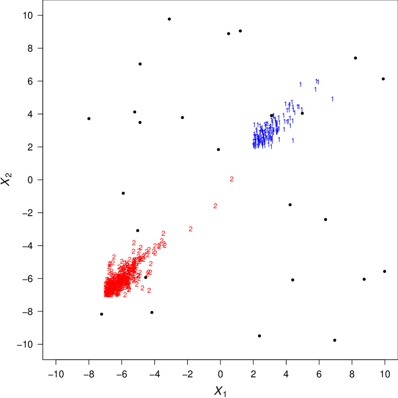
Figure 3: Simulated data from Section 5.2.1. Scatter plot (1 and 2 denote the first and second group, respectively). Background uniform noise points are denoted by $\bullet$.

Note that when a noise point effectively falls inside a cluster, which seems to happen at least three times (see Figure 3), we would expect it to be classified as belonging to the associated cluster.

The competing models are fitted to the generated data for $G\in\left\{1,2,3,4\right\}$, resulting in a total of 36 fitted models. The corresponding BIC values are reported in Table 4. The best (highest) BIC value for each family of models is highlighted in bold, while the overall best BIC value is highlighted in bold-italic.

Table 4: Simulated data from Section 5.2.1. BIC values for the fitted models. The best BIC value for each column is highlighted in bold, while the overall best in bold-italic.

$G$		N	$t$	CN	SN	S$t$	SCN	SS	SAL	CSAL
$1$		-5253.407	-4186.751	-4181.329	-4901.628	-3727.904	-3816.015	-3894.781	-4060.942	-3755.484
$2$		-3564.567	-2977.244	-3041.134	-3464.250	-2862.409	-2910.145	-3015.825	-3084.261	-2829.773
$3$		-2969.665	-2931.081	-2990.333	-2918.205	-2854.732	-2834.897	-2940.549	-2991.041	-2886.742
$4$		-2887.413	-2894.023	-2936.557	-2858.626	-2861.371	-2890.005	-2971.456	-3005.068	-2927.472

For each considered family, the scatter plot of the best model according to the BIC, along with the MAP-classification of the observations, is graphically represented in Figure 4.

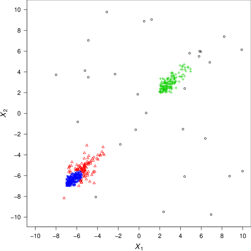
(a) N mixture with $G=4$

(b) $t$ mixture with $G=4$

(c) CN mixture with $G=4$

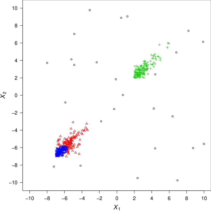
(d) SN mixture with $G=4$

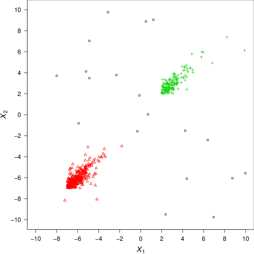
(e) S$t$ mixture with $G=3$

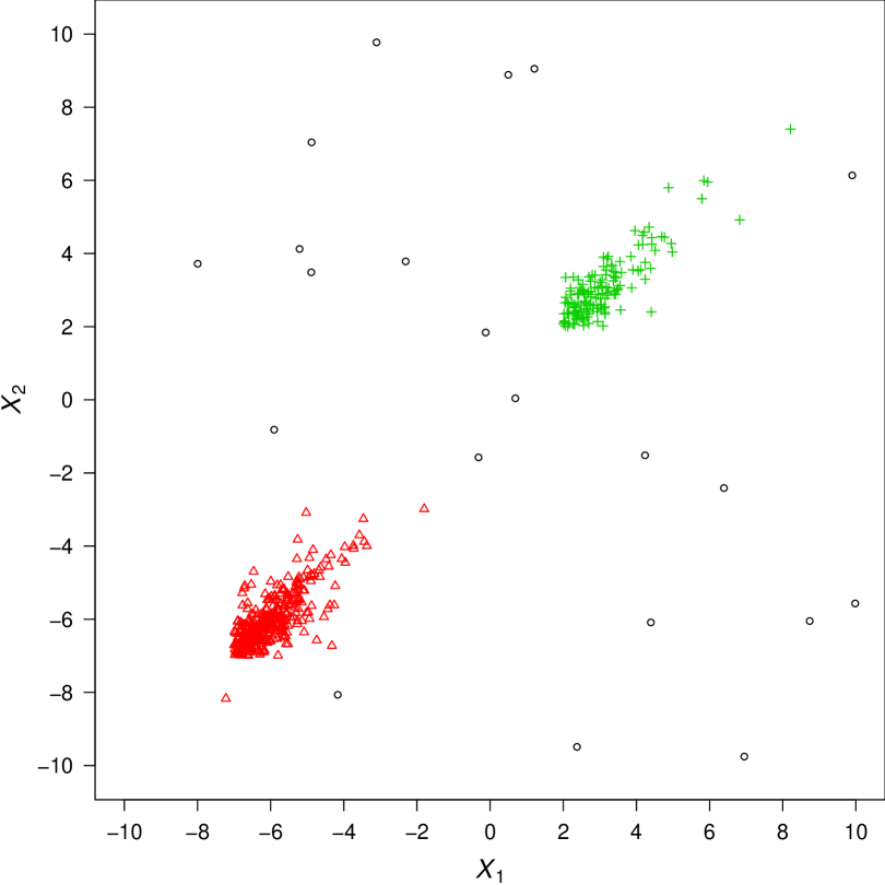
(f) SCN mixture with $G=3$

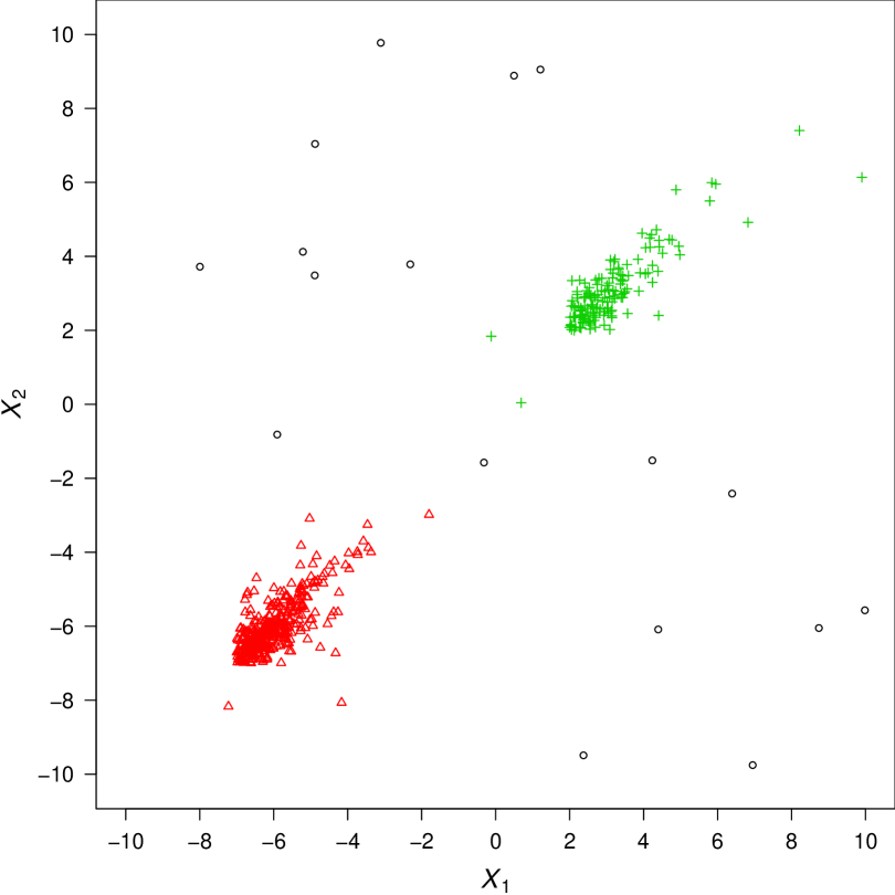
(g) SS mixture with $G=3$

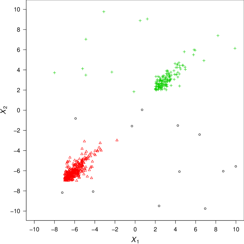
(h) SAL mixture with $G=3$

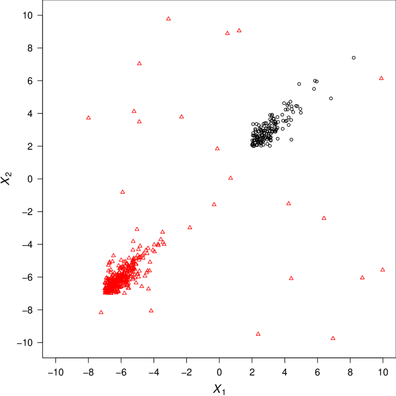
(i) CSAL mixture with $G=2$

Figure 4: Simulated data from Section 5.2.1. Scatter plots and MAP-classification of the observations from the models selected by the BIC.

The BIC selects $G=4$ clusters for the mixtures with elliptically symmetric (N, $t$ and CN) components. For these models, one component fits the cluster on the top-right, two components are needed to reproduce the asymmetric shape of the cluster on the bottom-left, and another component is attempting to model the background noise (see Figures 4(a)–4(c)). Surprisingly, the BIC selects $G=4$ components for the SN mixture too (see Figure 4(d)); the MAP-classification of the observations from this model is analogous to the previous ones meaning that the empirical skewness of the cluster on the bottom-left is not well-reproduced by the skewness of a single SN distribution. Apart from the CSAL mixture, the BIC selects $G=3$ clusters for all the other (S$t$, SCN, SS and SAL) mixtures. By looking at Figures 4(e)–4(h), two components of these mixtures fit the two clusters, as well as part of the background noise (although with a different extent depending on the model), and the additional component models the remaining part of the background noise. Finally, the BIC selects $G=2$ components for the CSAL mixture; for this model, the tails of the component on the bottom-left capture a great part of the background noise (see Figure 4(i)). The mixture of two CSAL distributions is, overall, the best fitted model according to the BIC (see Table 4).

In terms of classification performance, we first analyze the behavior of the competing models in classifying the good data and then we evaluate the ability of the mixtures with contaminated components in detecting the background noise. As concerns the first part of this analysis, Table 5 reports the confusion matrices between the true and predicted MAP-classification from each model selected by the BIC. Note that confusion matrices are computed only with respect to the 500 true good observations.

Table 5: Simulated data from Section 5.2.1. Confusion matrices, with respect to the good data only, from the models selected by the BIC.

	Fitted
True	1	2	3	4
1	144	6	0	0
2	0	3	103	244

(a) N mixture

	Fitted
True	1	2	3	4
1	144	6	0	0
2	0	3	106	241

(b) $t$ mixture

	Fitted
True	1	2	3	4
1	144	6	0	0
2	0	3	116	231

(c) CN mixture

	Fitted
True	1	2	3	4
1	148	2	0	0
2	0	3	121	226

(d) SN mixture

	Fitted
True	1	2	3
1	150	0	0
2	0	2	348

(e) S$t$ mixture

	Fitted
True	1	2	3
1	150	0	0
2	0	2	348

(f) SCN mixture

	Fitted
True	1	2	3
1	150	0	0
2	1	1	348

(g) SS mixture

	Fitted
True	1	2	3
1	150	0	0
2	0	2	348

(h) SAL mixture

	Fitted
True	1	2
1	150	0
2	0	350

(i) CSAL mixture

We highlight that the two underlying groups of good data are classified correctly by the CSAL mixture only ($\text{ARI}=1$); see Table 6(i). The selected N mixture roughly splits the second group in two sub-clusters, while the cluster devoted to the background noise also absorbs 6 observations from group 1, and 3 observations from group 2 ($\text{ARI}=0.584$); see Table 6(a). Similar results are obtained for $t$, CN and SN mixtures, with ARI values equal to 0.578, 0.560 and 0.561, respectively; see Tables 6(b)–6(d). For the mixture models with $G=3$ skewed (S$t$, SCN, SS and SAL) clusters, selected by the BIC, the first group is classified correctly, in the sense that it is not split by the fitted models in sub-groups; however, some (one or two) of the observations in the second group are assigned to the noise component of these models and, for the SS mixture, one observation from group 2 is joined to the first component of the mixture. The ARI values for these models are high (0.989 for S$t$, SCN and SAL mixtures, and 0.986 for the SS mixture). The CSAL mixture selected by the BIC is the best performer, in terms of classification of the good data, being the only one producing a correct number of mixture components and a perfect classification ($\text{ARI}=1$).

For the purpose of evaluation of the performance of the competing mixtures of contaminated distributions in detecting the background noise, we report the true positive rate (TPR), measuring the proportion of bad points that are correctly identified as bad points, and the false positive rate (FPR), corresponding to the proportion of good points incorrectly classified as bad points. We consider the fitted CN, SCN, and CSAL mixtures with $G=2$ components. We use the outlier detection rule detailed in Punzo and McNicholas (2016) for the CN mixture, and the detection rule illustrated in Section 4.6 for the CSAL mixture. The underlying principle of these rules is the same. We apply an analogous outlier detection rule for the SCN mixture; to our knowledge, this is the first time such a detection rule is used on the SCN mixture proposed by Cabral et al. (2012). Table 6 reports the obtained TPRs and FPRs from the three model-based outlier detection rules.

Table 6: Simulated data from Section 5.2.1. TPRs and FPRs from the CN, SCN and CSAL mixtures with $G=2$ components.

	CN mixture	SCN mixture	CSAL mixture
TPR	0.920	0.880	0.800
FPR	0.106	0.032	0.004

The CN mixture shows the highest TPR, while the CSAL mixture gives the lowest (almost optimal) FPR. To find out more about the motivation of these results, Figure 5 shows, for each of the three mixtures of contaminated distributions, the scatter plot of the observations with symbols and colors diversified with respect to the group MAP-membership; detected outliers are denoted by bullets.

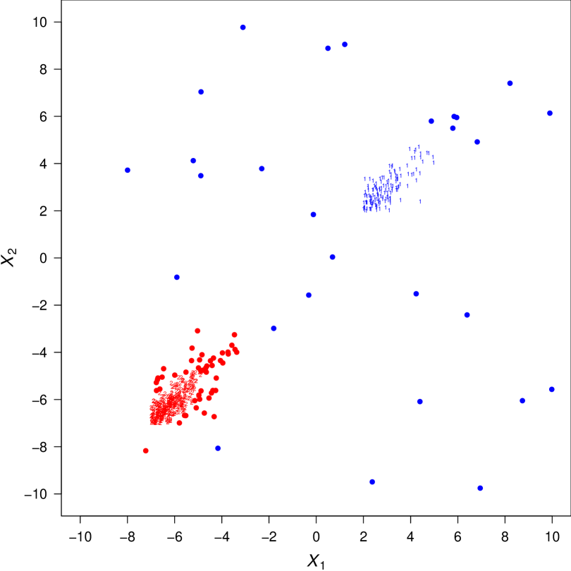
(a) CN mixture

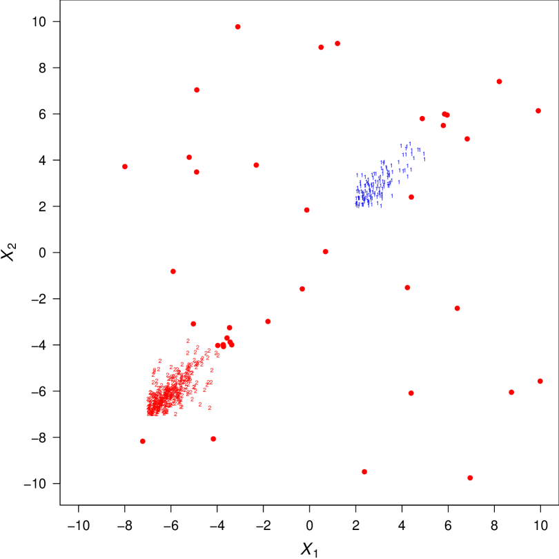
(b) SCN mixture

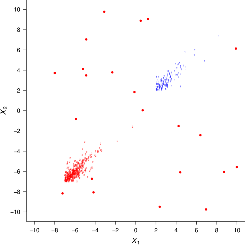
(c) CSAL mixture

Figure 5: Simulated data from Section 5.2.1. Scatter plots and MAP-classification of the observations from the CN, SCN and CSAL mixtures with $G=2$ clusters. Bullets denote detected bad points.

The FPR from the CN mixture is high (0.106) because a lot of good observations on the boundary of the bottom-left group are seen as outliers by the CN density of that cluster. In detail, an “elliptical” subset of the group is accommodated by the good component of the CN density, while the rest is banished to the bad one. For this CN component, the estimated proportion of good points is 0.778 while the corresponding degree of contamination is 5.824. By comparing Figure 3 with Figure 5(a), the CN mixture behaves in a similar way, even if with a lower extent, on the top-right group. However, the bad component of the CN distribution is now more devoted to capture the background noise. This is confirmed by an high estimated degree of contamination (20.889), which is greater than the degree of contamination (5.824) of the other CN mixture component; the estimated proportion of good observations is now 0.811. The FPR, equal to 0.032, from the SCN mixture is due to the fact the long north-east tail of both the groups of good data is instead seen as composed by outliers by the model. The “low” TPR from the CSAL mixture is 0.800 is mainly due to two reasons. Firstly, some of the added noise points end up in the interior of the groups (see Figure 3), making it difficult to identify them as outliers by any detection rule. Secondly, the two good SAL components of the two CSAL distributions of the mixture are, by theirself, already able to cope with a certain fraction of the background noise. The remaining part of the noise is captured by the bad SAL component of the CSAL distribution located on the bottom-left. This distribution has an estimated proportion of good data equal to $\hat{\lambda}_{2}=0.940$ and a high estimated degree of contamination ($\hat{\rho}_{2}=331.409$).

5.2.2 Example with $G=3$ groups and $p=2$ dimensions

In the second example, $n=1000$ bivariate ($p=2$) observations are generated by a mixture of $G=3$ $t$-slice distributions with parameters

$$\pi_{1}=0.5,\ \pi_{2}=0.2,\ \boldsymbol{\mu}_{1}=\begin{bmatrix}[c]-7\\ -7\end{bmatrix},\ \boldsymbol{\mu}_{2}=\begin{bmatrix}[c]2\\ 2\end{bmatrix},\ \boldsymbol{\mu}_{3}=\begin{bmatrix}[c]11\\ 11\end{bmatrix},\ \boldsymbol{\Sigma}_{1}=\boldsymbol{\Sigma}_{2}=\boldsymbol{\Sigma}_{3}=\begin{bmatrix}[c]1&0.9\\ 0.9&1\end{bmatrix},\ \text{and}\ \nu_{1}=\nu_{2}=\nu_{3}=6.$$

As for the the example in Section 5.2.1, 50 noise points are added from a uniform distribution over the interval $(-10,10)$ on each dimension. The scatter plot of the generated data, with labels 1, 2 and 3 for points from the first, second and third group, respectively, and with bullets denoting uniform noise points, is displayed in Figure 6.

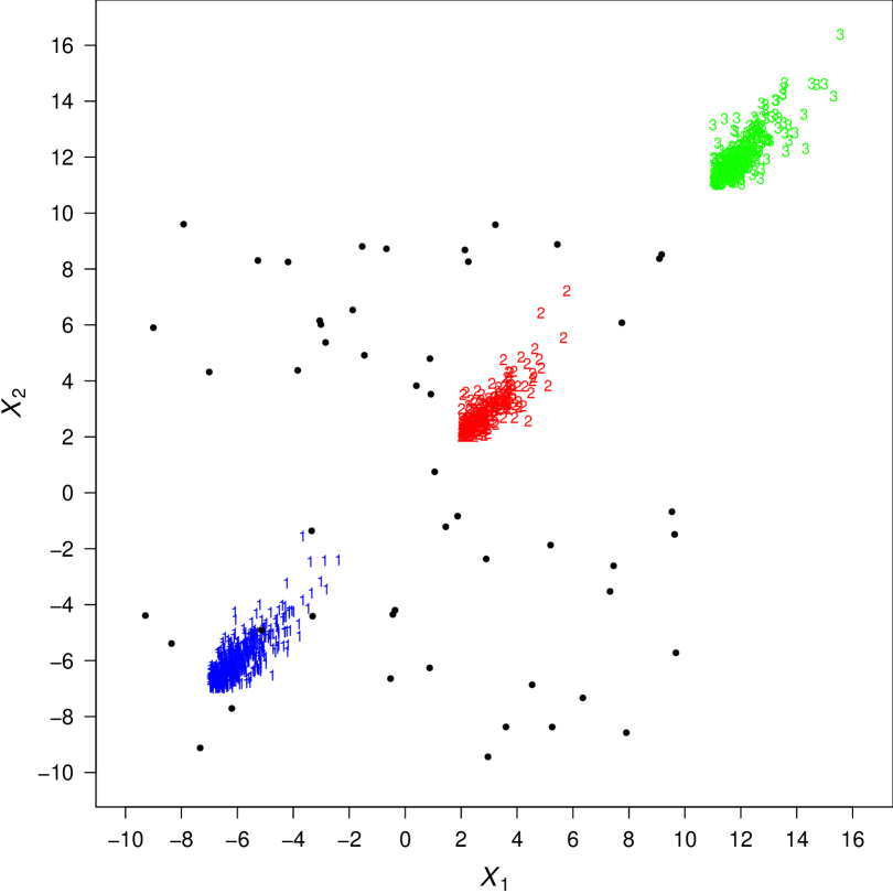
Figure 6: Simulated data from Section 5.2.2. Scatter plot (1, 2 and 3 denote the first, second and third group, respectively). Background uniform noise points are denoted by $\bullet$.

As we can see, in this example the noise covers only two of the three generated clusters.

The competing models are fitted to the generated data for $G\in\left\{1,2,3,4,5\right\}$. The corresponding BIC values are reported in Table 7.

Table 7: Simulated data from Section 5.2.2. BIC values for the fitted models. The best BIC value for each column is highlighted in bold, while the overall best in bold-italic.

$G$		N	$t$	CN	SN	S$t$	SCN	SS	SAL	CSAL
$1$		-11698.509	-9947.977	-9659.884	-11138.797	-9172.015	-9076.360	-9675.003	-10634.259	-10036.071
$2$		-9180.156	-8143.511	-7889.729	-8838.385	-7687.617	-7944.347	-8220.684	-8167.903	-7629.978
$3$		-7607.284	-6788.780	-6850.640	-7340.803	-6534.969	-6530.765	-6647.791	-6777.626	-6435.498
$4$		-7490.312	-6634.094	-6654.045	-6487.831	-6575.936	-6559.681	-6473.617	-6459.348	-6512.047
$5$		-6752.651	-6651.128	-6737.504	-7385.226	-6608.633	-6549.832	-6504.393	-6468.838	-6535.544

We can note how the best model, among the 45 models being fitted, is the CSAL mixture with $G=3$ clusters. For the models selected by the BIC, Table 8 reports the corresponding ARI values with respect to the good points only.

Table 8: Simulated data from Section 5.2.2. ARI values, on the good data only, for the mixture models selected by the BIC.

		N	$t$	CN	SN	S$t$	SCN	SS	SAL	CSAL
$G$		5	4	4	4	3	3	4	4	3
ARI		0.970	0.996	0.994	0.980	1.000	0.988	0.997	0.310	1.000

The S$t$ and CSAL mixtures attain a perfect classification ($\text{ARI}=1$), while the SAL mixture is the model with the worst classification results ($\text{ARI}=0.310$).

Table 9 reports TPRs and FPRs from the application of the outlier detection rules from the fitted CN, SCN, and CSAL mixtures with $G=3$ clusters.

Table 9: Simulated data from Section 5.2.2. TPRs and FPRs from the CN, SCN and CSAL mixtures with $G=3$ components.

	CN mixture	SCN mixture	CSAL mixture
TPR	0.940	0.940	0.940
FPR	0.080	0.025	0.001

The competing rules provide the same TPR (0.940), but the rule associated to the CSAL mixture is the one providing the best, almost perfect, FPR (0.001), followed by the rule associated to the SCN mixture ($\text{FPR}=0.025$). Figure 7 shows, for each of the three mixtures of contaminated distributions, the scatter plot of the observations with symbols and colors diversified with respect to the group MAP-membership; detected outliers are denoted by bullets.

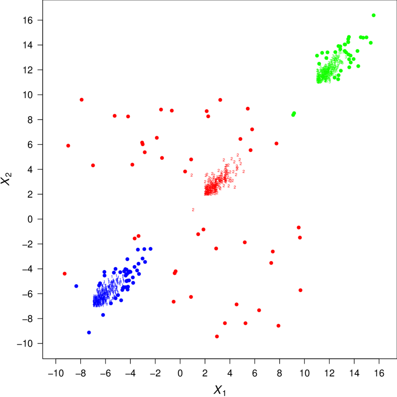
(a) CN mixture

(b) SCN mixture

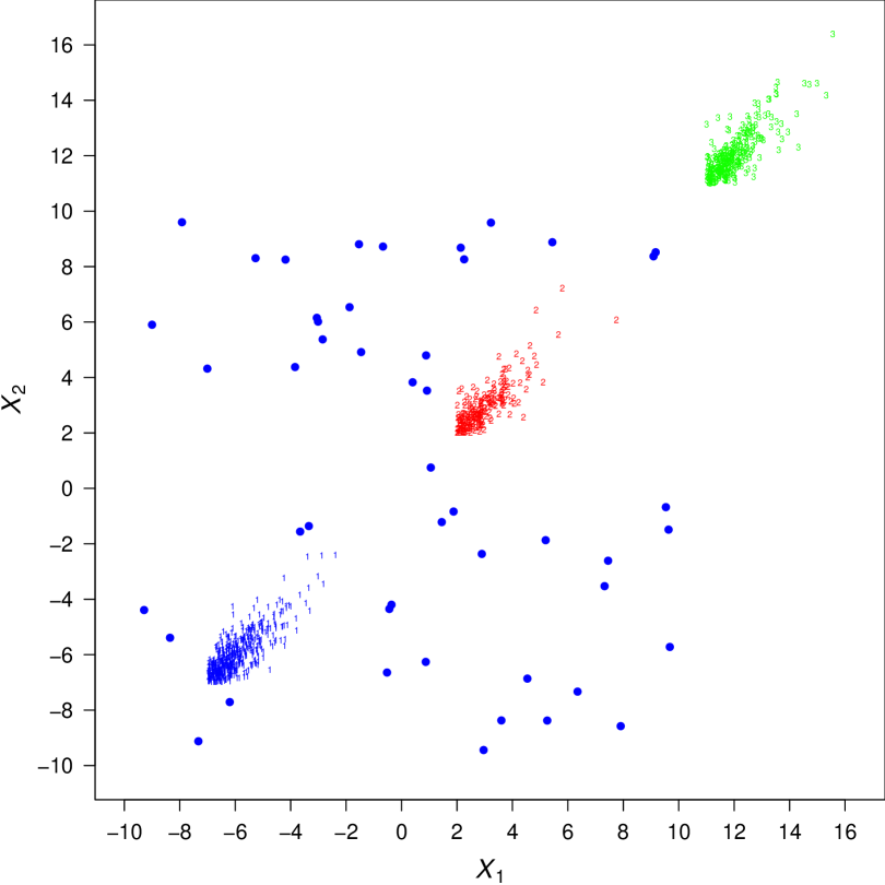
(c) CSAL mixture

Figure 7: Simulated data from Section 5.2.2. Scatter plots and MAP-classification of the observations from the CN, SCN and CSAL mixtures with $G=3$ clusters. Bullets denote detected bad points.

As we can note, the considered models place their three components on the three underlying groups of good data. However, their way to declare observations as outliers is different. For the CN mixture, the bad component of the CN density on the middle accommodates a great part of the background noise. Instead, the bad components of the two remaining CN densities accommodate the external part of the groups composed by good observations, and this contributes to increase the FPR for this model. As concerns the SCN mixture, a part of the background noise is accommodated by the bad component of the SCN density on the bottom-left, while the remaining part is accommodated by the SCN density on the middle. However, some good observations in the north-east direction of the groups on the bottom-left and the top-right are seen as outliers too, and this is the motivation of the non-optimal FPR for the detection rule from this model. Instead, an almost perfect detecting behavior is observed for the CSAL mixture, with the bad component of the CSAL density on the bottom-left capturing all the background noise; with reference to this cluster of the CSAL mixture, the estimated mixture weight is $\hat{\pi}_{1}=0.524$, the estimated proportion of good data is $\hat{\lambda}_{1}=0.902$, and the estimated degree of contamination is $\hat{\rho}_{1}=182.088$.

5.2.3 Example with $G=2$ groups and $p=3$ dimensions

In the third example, $n=500$ trivariate ($p=3$) observations are generated by a mixture of $G=2$ $t$-slice distributions with parameters

$$\pi_{1}=0.7,\quad\boldsymbol{\mu}_{1}=\begin{bmatrix}[c]-7\\ -7\\ -7\end{bmatrix},\quad\boldsymbol{\mu}_{2}=\begin{bmatrix}[c]11\\ 11\\ 11\end{bmatrix},\quad\boldsymbol{\Sigma}_{1}=\boldsymbol{\Sigma}_{2}=\begin{bmatrix}[c]1&0.9&0.9\\ 0.9&1&0.9\\ 0.9&0.9&1\end{bmatrix},\quad\text{and}\quad\nu_{1}=\nu_{2}=6.$$

Moreover, 25 noise points are added from a uniform distribution over the interval $(-10,10)$ on each dimension. The matrix of pairwise scatter plots of the generated data, with labels 1 and 2 for points from the first and second group, respectively, and with bullets denoting uniform noise points, is displayed in Figure 8.

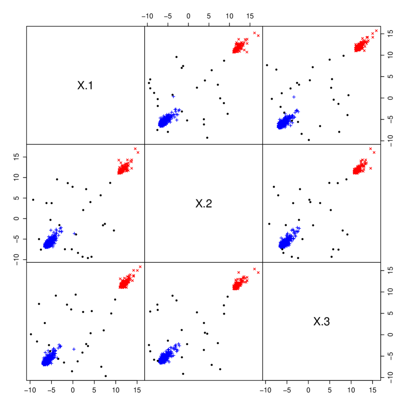
Figure 8: Simulated data from Section 5.2.3. Matrix of pairwise scatter plots ($+$ and $\times$ denote the first and second groups, respectively). Background uniform noise points are denoted by $\bullet$.

As we can see, the noise covers only one of the two generated clusters.

The competing models are fitted to the generated data for $G\in\left\{1,2,3,4\right\}$. The corresponding BIC values are reported in Table 10.

Table 10: Simulated data from Section 5.2.3. BIC values for the fitted models. The best BIC value for each column is highlighted in bold, while the overall best in bold-italic.

$G$		N	$t$	CN	SN	S$t$	SCN	SS	SAL	CSAL
1		-7913.407	-5869.537	-5774.226	-7513.308	-5363.720	-5363.330	-5486.237	-5988.705	-5506.787
2		-6494.045	-3861.820	-3870.294	-6058.756	-3698.826	-3774.388	-3719.261	-4186.362	-3660.907
3		-3905.722	-3796.367	-3807.067	-3780.592	-3671.086	-3710.395	-3701.616	-3672.434	-3708.272
4		-3786.715	-3748.906	-3776.244	-3762.349	-3724.686	-3791.960	-3762.420	-3747.273	-3789.211

The best fitted model is the CSAL mixture with $G=2$ clusters. For the models selected by the BIC, Table 11 shows the corresponding ARI values with respect to the good data only.

Table 11: Simulated data from Section 5.2.3. ARI values, on the good data only, for the mixture models selected by the BIC.

		N	$t$	CN	SN	S$t$	SCN	SS	SAL	CSAL
$G$		4	4	4	4	3	3	3	3	2
ARI		0.564	0.532	0.563	0.638	0.994	0.994	0.994	0.977	1.000

The CSAL mixture is the only model attaining a perfect classification ($\text{ARI}=1$), followed by the S$t$, SCN and SS mixtures sharing the same ARI value (0.994). The model with the worst classification results is the $t$ mixture ($\text{ARI}=0.532$).

Table 12 reports TPRs and FPRs from the application of the outlier detection rules from the fitted CN, SCN, and CSAL mixtures with $G=2$ components.

Table 12: Simulated data from Section 5.2.3. TPRs and FPRs from the CN, SCN and CSAL mixtures with $G=2$ components.

	CN mixture	SCN mixture	CSAL mixture
TPR	1.000	1.000	1.000
FPR	0.066	0.028	0.002

The competing outlier detection rules provide an optimal TPR (1.000), but the rule from the CSAL mixture is the one providing the best, almost perfect, FPR (0.002), followed by the rules from the SCN mixture ($\text{FPR}=0.028$) and CN mixture ($\text{FPR}=0.066$). Thus, the outlier detection rule from the CSAL mixture dominates, in terms of performance, the competing rules. Figure 9 shows, for the CSAL mixture with $G=2$ clusters only, the matrix of scatter plots of the observations with symbols and colors diversified with respect to the group MAP-membership; detected outliers are denoted by bullets.

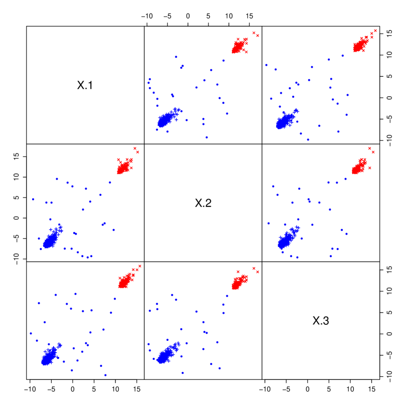
Figure 9: Simulated data from Section 5.2.3. Matrix of pairwise scatter plots with MAP-classification of the observations from the CSAL mixture with $G=2$ components. Bullets denote detected bad points.

As we can note by comparing Figure 9 with Figure 8, the model is able to reproduce the underlying group-structure and to detect the background noise. In particular, the noise is entirely captured by the bad component of the CSAL pdf placed on the bottom-left group; with reference to this component of the CSAL mixture, the estimated mixture weight is $\hat{\pi}_{1}=0.715$, the estimated proportion of good data is $\hat{\lambda}_{1}=0.925$ and the estimated degree of contamination is $\hat{\rho}_{1}=271.767$. The estimated proportion of good data in the other CSAL mixture component (i.e., $\hat{\lambda}_{2}$) is approximately equal to 1.

5.3 The bankruptcy data set

This real data analysis considers the bankruptcy data set (Altman, 1968) containing, for $n=66$ manufacturing firms in the United States, the values of $p=2$ variables: the ratio of retained earnings (RE) to total assets, and the ratio of earnings before interests and taxes (EBIT) to total assets. Half of the selected firms had filed for bankruptcy. This data set accompanies the ManlyMix package (Zhu and Melnykov, 2017) for R. The goal here is to predict whether a firm went bankrupt based on the two variables. Under the same goal, this data set has been already used in the literature as an illustrative example for clustering methods assuming skewed and/or leptokurtic clusters (e.g., Lo and Gottardo, 2012 and McNicholas, 2016a, Chapter 7).

Figure 10 shows the scatter plot of the data, where solvent and bankrupted firms are labeled as $\times$ and $\circ$, respectively.

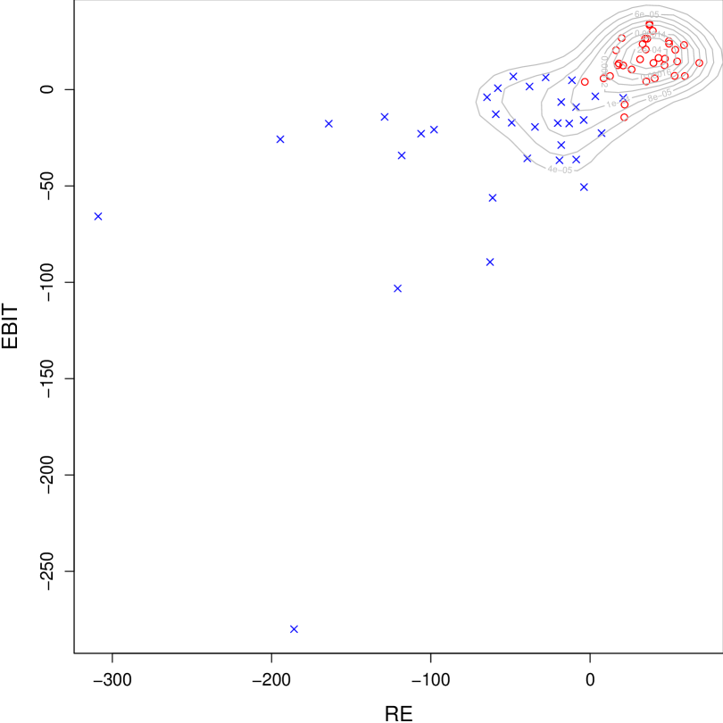
Figure 10: Bankruptcy data set: scatter plot of RE and EBIT ($\times$ denotes the solvent firms and $\circ$ the bankrupted ones) along with contours from a bivariate normal kernel estimator.

Table 13: Bankruptcy data set: log-likelihood, BIC, and classification performance from various mixture models with $G=2$ clusters. Bold font highlights the best value for each column.

Mixture components	Log-likelihood	BIC	# misclassified	Error rate	ARI
N	-652.049	-1350.185	21	0.318	0.124
$t$	-646.296	-1342.869	4	0.061	0.769
CN	-643.339	-1349.522	5	0.076	0.716
SN	-636.739	-1336.322	16	0.242	0.257
S$t$	-633.989	-1335.013	14	0.212	0.323
SCN	-631.301	-1333.826	14	0.212	0.323
SS	-635.874	-1338.782	15	0.227	0.289
SAL	-642.016	-1346.877	24	0.364	0.068
CSAL	-630.944	-1341.491	3	0.045	0.824

The contours from a bivariate normal kernel estimator, as implemented by the bkde2D() function of the KernSmooth package (Wand, 2015), are also superimposed on the scatter plot. By looking at Figure 10, the bivariate sample is apparently bimodal, justifying the fit of two-component mixture models, with seemingly skewed clusters and possible outliers.

Table 13 presents a model comparison in terms of BIC values and shows some measures of agreement between the partition provided by each fitted model with respect to the known classification of the firms as solvent and bankrupted.

As can be seen, the SCN mixture is the best model according to the BIC, followed by the S$t$ and SN mixtures. The CSAL mixture occupies the fifth position in this ranking. If we take a look at the results of Table 13 from a classification point of view, the ranking changes a lot. The worst classification result is obtained for the SAL mixture (with 24 misclassified firms), while the best one is attained by the CSAL mixture (with only 3 misclassified firms). Interestingly, the models based somehow on the SAL distribution occupy the extremes of this ranking; this highlights how the contaminated generalization of the SAL mixture we provide can contribute to improve the classification performance of the SAL mixture. Note also that, the classification from the CSAL mixture is even better than the one from the models compared by Lo and Gottardo (2012). The second best model, with 4 misclassified firms, is the $t$ mixture, followed by the CN mixture with 5 misclassified firms. The other competing models have more than 13 misclassified firms each. Thus, the best three models have leptokurtic clusters; however, allowing for skewed clusters helps the CSAL mixture to attain better classification results.

The partition from the CSAL mixture, along with its contours, is depicted in Figure 11, where an arrow indicates the unique outlier detected by the model; it belongs to the group of the solvent firms whose members are denoted with 1 in Figure 11.

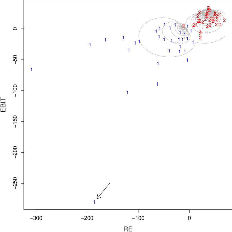
Figure 11: Bankruptcy data set: scatter plot of RE and EBIT with classification and contours from the fitted two-component CSAL mixture. The arrow indicates the unique firm detected as outlier by the model.

For the detected outlier it is also important to underline that its a posteriori probability to be good, in its MAP group of membership (group 1), is practically null. By looking at Figure 11, there seems to be another firm, on the extreme left, which could be deemed, to eye, as an outlier, especially if one considers its distance from the bulk of the RE values. For this point, the a posteriori probability to be good, in its MAP group of membership (which is group 1), is 0.748. This high enough probability to be good is justified if one considers the high left skewness with respect to RE induced by the first element of the estimated parameter vector $\hat{\boldsymbol{\alpha}}_{1}=\left(-56.947,-22.096\right)^{\top}$. Finally note that, in the group containing the outlier, the estimated proportion of good points is $\hat{\lambda}_{1}=0.932$ and the degree of contamination is $\hat{\rho}_{1}=418.872$; the so high value of $\hat{\rho}_{1}$ is manly due to the distance of the detected outlier from the bulk of group 1.

6 Conclusions

This paper introduced mixtures of contaminated shifted asymmetric Laplace (CSAL) distributions as a model-based clustering method for handling asymmetric clusters under the presence of outliers. Each component (cluster) of the mixture of CSAL distributions is a two-component SAL mixture in which one of the components, with a large prior probability, represents the “good” observations, and the other, with a small prior probability, with the same mode and an inflated covariance matrix — obtained by including a contamination factor altering the skewness and scale parameters — represents the “bad” observations. Advantageously, each mixture component is unimodal. The ECM algorithm was employed to classify an observation by first determining its group membership, and then establishing whether it is an outlier (or otherwise bad point) within that group. The method was applied to simulated and real data where it yielded good results when outliers (artificial or natural) were present. The procedure was benchmarked against other well-established mixture models, and it outperformed them, with respect to various aspects, in most of the data sets considered.

As an open point for further research, following the idea of McLachlan et al. (2003), McNicholas and Murphy (2008), and Subedi et al. (2013) for mixtures using the normal distribution, McLachlan et al. (2007), Andrews and McNicholas (2011), and Subedi et al. (2015) for mixtures using the $t$ distribution, Punzo and McNicholas (2014) for contaminated normal mixtures, and Murray et al. (2014b) for mixture using the skew-$t$ distribution, parsimony, but also dimension reduction, could be introduced into the model by exploiting local factor analyzers; this would lead to mixtures of CSAL factor analyzers. As a further possibility for further work, it would be of interest to extend the current approach to accommodate missing values in the fashion, for instance, of Lin et al. (2006, 2009) and Lin (2014).

References

- Aitken (1926) Aitken, A. C. (1926). On Bernoulli’s numerical solution of algebraic equations. In Proceedings of the Royal Society of Edinburgh, Volume 46, pp. 289–305.
- Aitkin and Wilson (1980) Aitkin, M. and G. T. Wilson (1980). Mixture models, outliers, and the EM algorithm. Technometrics 22(3), 325–331.
- Altman (1968) Altman, E. I. (1968). Financial ratios, discriminant analysis and the prediction of corporate bankruptcy. Journal of Finance 23(4), 589–609.
- Andrews and McNicholas (2011) Andrews, J. L. and P. D. McNicholas (2011). Extending mixtures of multivariate -factor analyzers. Statistics and Computing 21(3), 361–373.
- Azzalini (2005) Azzalini, A. (2005). The skew-normal distribution and related multivariate families. Scandinavian Journal of Statistics 32(2), 159–188.
- Azzalini and Capitanio (2014) Azzalini, A. and A. Capitanio (2014). The Skew-Normal and Related Families, Volume 3 of IMS monographs. Cambridge University Press.
- Bagnato and Punzo (2013) Bagnato, L. and A. Punzo (2013). Finite mixtures of unimodal beta and gamma densities and the -bumps algorithm. Computational Statistics 28(4), 1571–1597.
- Bagnato et al. (2017) Bagnato, L., A. Punzo, and M. G. Zoia (2017). The multivariate leptokurtic-normal distribution and its application in model-based clustering. Canadian Journal of Statistics 45(1), 95–119.
- Basso et al. (2010) Basso, R. M., V. H. Lachos, C. R. B. Cabral, and P. Ghosh (2010). Robust mixture modeling based on scale mixtures of skew-normal distributions. Computational Statistics & Data Analysis 54(12), 2926–2941.
- Berger and Berliner (1986) Berger, J. and L. M. Berliner (1986). Robust Bayes and empirical Bayes analysis with -contaminated priors. The Annals of Statistics 14(2), 461–486.
- Berkane and Bentler (1988) Berkane, M. and P. M. Bentler (1988). Estimation of contamination parameters and identification of outliers in multivariate data. Sociological Methods & Research 17(1), 55–64.
- Biernacki et al. (2003) Biernacki, C., G. Celeux, and G. Govaert (2003). Choosing starting values for the EM algorithm for getting the highest likelihood in multivariate Gaussian mixture models. Computational Statistics & Data Analysis 41(3-4), 561–575.
- Böhning et al. (1994) Böhning, D., E. Dietz, R. Schaub, P. Schlattmann, and B. G. Lindsay (1994). The distribution of the likelihood ratio for mixtures of densities from the one-parameter exponential family. Annals of the Institute of Statistical Mathematics 46(2), 373–388.
- Brazier et al. (1983) Brazier, S., R. S. J. Sparks, S. N. Carey, H. Sigurdsson, and J. A. Westgate (1983). Bimodal Grain Size Distribution and Secondary Thickening in Air-Fall Ash Layers. Nature 301, 115–119.
- Browne and McNicholas (2015) Browne, R. P. and P. D. McNicholas (2015). A mixture of generalized hyperbolic distributions. Canadian Journal of Statistics 43(2), 176–198.
- Cabral et al. (2012) Cabral, C. S. B., V. H. Lachos, and M. O. Prates (2012). Multivariate mixture modelling using skew-normal independent distributions. Computational Statistics & Data Analysis 56, 126–142.
- da Silva Ferreira et al. (2011) da Silva Ferreira, C., H. Bolfarine, and V. H. Lachos (2011). Skew scale mixtures of normal distributions: properties and estimation. Statistical Methodology 8(2), 154–171.
- Dang et al. (2015) Dang, U. J., R. P. Browne, and P. D. McNicholas (2015). Mixtures of multivariate power exponential distributions. Biometrics 71(4), 1081–1089.
- Dasgupta and Raftery (1998) Dasgupta, A. and A. E. Raftery (1998). Detecting features in spatial point processes with clutter via model-based clustering. Journal of the American Statistical Association 93(441), 294–302.
- Dempster et al. (1977) Dempster, A. P., N. M. Laird, and D. B. Rubin (1977). Maximum likelihood from incomplete data via the EM algorithm. Journal of the Royal Statistical Society: Series B (Statistical Methodology) 39(1), 1–38.
- Dharmadhikari and Joag-Dev (1988) Dharmadhikari, S. and K. Joag-Dev (1988). Unimodality, Convexity, and Applications. Probability and Mathematical Statistics. Elsevier Science.
- Fraley and Raftery (2002) Fraley, C. and A. E. Raftery (2002). Model-based clustering, discriminant analysis, and density estimation. Journal of the American statistical Association 97(458), 611–631.
- Franczak (2014) Franczak, B. C. (2014). Mixtures of Shifted Asymmetric Laplace Distributions. Ph.D. thesis, University of Guelph.
- Franczak et al. (2014) Franczak, B. C., R. P. Browne, and P. D. McNicholas (2014). Mixtures of shifted asymmetric Laplace distributions. IEEE Transactions on Pattern Analysis and Machine Intelligence 36(6), 1149–1157.
- Gallegos and Ritter (2009) Gallegos, M. T. and G. Ritter (2009). Trimmed ML estimation of contaminated mixtures. Sankhyā: The Indian Journal of Statistics, Series A 71(2), 164–220.
- Gutierrez et al. (1995) Gutierrez, R. G., R. J. Carroll, N. Wang, G. H. Lee, and B. H. Taylor (1995). Analysis of tomato root initiation using a normal mixture distribution. Biometrics 51(4), 1461–1468.
- Hall and Hall (2017) Hall, B. and M. Hall (2017). LaplacesDemon: Complete Environment for Bayesian Inference. Version 16.1.0.
- Hubert and Arabie (1985) Hubert, L. and P. Arabie (1985). Comparing partitions. Journal of Classification 2(1), 193–218.
- Karlis and Santourian (2009) Karlis, D. and A. Santourian (2009). Model-based clustering with non-elliptically contoured distributions. Statistics and Computing 19(1), 73–83.
- Karlis and Xekalaki (2003) Karlis, D. and E. Xekalaki (2003). Choosing initial values for the EM algorithm for finite mixtures. Computational Statistics & Data Analysis 41(3–4), 577–590.
- Keribin (2000) Keribin, C. (2000). Consistent estimation of the order of mixture models. Sankhyā: The Indian Journal of Statistics, Series A 62(1), 49–66.
- Kotz et al. (2012) Kotz, S., T. Kozubowski, and K. Podgorski (2012). The Laplace Distribution and Generalizations: A Revisit with Applications to Communications, Economics, Engineering, and Finance. SpringerLink: Bücher. Birkhäuser Boston.
- Lachos et al. (2010) Lachos, V. H., P. Ghosh, and R. B. Arellano-Valle (2010). Likelihood based inference for skew-normal independent linear mixed models. Statistica Sinica 20(1), 303–322.
- Lachos and Labra (2014) Lachos, V. H. and F. V. Labra (2014). Multivariate skew-normal/independent distributions: properties and inference. Pro Mathematica 28(56), 11–53.
- Lee and McLachlan (2014) Lee, S. X. and G. J. McLachlan (2014). Finite mixtures of multivariate skew -distributions: some recent and new results. Statistics and Computing 24(2), 181–202.
- Lin (2009) Lin, T.-I. (2009). Maximum likelihood estimation for multivariate skew normal mixture models. Journal of Multivariate Analysis 100(2), 257–265.
- Lin (2010) Lin, T.-I. (2010). Robust mixture modeling using multivariate skew -distributions. Statistics and Computing 20, 343–356.
- Lin (2014) Lin, T.-I. (2014). Learning from incomplete data via parameterized mixture models through eigenvalue decomposition. Computational Statistics & Data Analysis 71, 183–195.
- Lin et al. (2009) Lin, T.-I., H. J. Ho, and P. S. Shen (2009). Computationally efficient learning of multivariate mixture models with missing information. Computational Statistics 24(3), 375–392.
- Lin et al. (2006) Lin, T.-I., J. C. Lee, and H. J. Ho (2006). On fast supervised learning for normal mixture models with missing information. Pattern Recognition 39(6), 1177–1187.
- Lin et al. (2007) Lin, T.-I., J. C. Lee, and S. Y. Yen (2007). Finite mixture modelling using the skew normal distribution. Statistica Sinica 17(3), 909–927.
- Lo and Gottardo (2012) Lo, K. and R. Gottardo (2012). Flexible mixture modeling via the multivariate distribution with the box-cox transformation: an alternative to the skew- distribution. Statistics and Computing 22(1), 33–52.
- Maruotti and Punzo (2017) Maruotti, A. and A. Punzo (2017). Model-based time-varying clustering of multivariate longitudinal data with covariates and outliers. Computational Statistics & Data Analysis 113, 475–496.
- Mazza and Punzo (2018) Mazza, A. and A. Punzo (2018). Mixtures of multivariate contaminated normal regression models. Statistical Papers.
- McLachlan and Krishnan (2007) McLachlan, G. and T. Krishnan (2007). The EM algorithm and extensions (Second ed.), Volume 382 of Wiley Series in Probability and Statistics. New York: John Wiley & Sons.
- McLachlan and Basford (1988) McLachlan, G. J. and K. E. Basford (1988). Mixture Models - Inference and Applications to Clustering. New York: Marcel Dekker.
- McLachlan et al. (2007) McLachlan, G. J., R. W. Bean, and L. B.-T. Jones (2007). Extension of the mixture of factor analyzers model to incorporate the multivariate -distribution. Computational Statistics & Data Analysis 51(11), 5327–5338.
- McLachlan and Peel (2000) McLachlan, G. J. and D. Peel (2000). Finite Mixture Models. New York: John Wiley & Sons.
- McLachlan et al. (2003) McLachlan, G. J., D. Peel, and R. W. Bean (2003). Modelling high-dimensional data by mixtures of factor analyzers. Computational Statistics & Data Analysis 41(3–4), 379–388.
- McNicholas (2016a) McNicholas, P. D. (2016a). Mixture Model-Based Classification. Boca Raton: Chapman & Hall/CRC Press.
- McNicholas (2016b) McNicholas, P. D. (2016b). Model-based clustering. Journal of Classification 33(3), 331–373.
- McNicholas and Murphy (2008) McNicholas, P. D. and T. B. Murphy (2008). Parsimonious Gaussian mixture models. Statistics and Computing 18, 285–296.
- McNicholas et al. (2010) McNicholas, P. D., T. B. Murphy, A. F. McDaid, and D. Frost (2010). Serial and parallel implementations of model-based clustering via parsimonious Gaussian mixture models. Computational Statistics & Data Analysis 54(3), 711–723.
- McNicholas et al. (2017) McNicholas, S. M., P. D. McNicholas, and R. P. Browne (2017). A mixture of variance-gamma factor analyzers. In S. E. Ahmed (Ed.), Big and Complex Data Analysis: Methodologies and Applications, pp. 369–385. Cham: Springer International Publishing.
- Meng and Rubin (1993) Meng, X.-L. and D. B. Rubin (1993). Maximum likelihood estimation via the ECM algorithm: A general framework. Biometrika 80(2), 267–278.
- Murphy (1964) Murphy, E. A. (1964). One Cause? Many Causes? The Argument from the Bimodal Distribution. Journal of Chronic Diseases 17(4), 301–324.
- Murray et al. (2014a) Murray, P. M., R. B. Browne, and P. D. McNicholas (2014a). Mixtures of skew-t factor analyzers. Computational Statistics and Data Analysis 77, 326–335.
- Murray et al. (2017a) Murray, P. M., R. B. Browne, and P. D. McNicholas (2017a). Hidden truncation hyperbolic distributions, finite mixtures thereof, and their application for clustering. Journal of Multivariate Analysis 161, 141–156.
- Murray et al. (2014b) Murray, P. M., R. P. Browne, and P. D. McNicholas (2014b). Mixtures of skew- factor analyzers. Computational Statistics & Data Analysis 77, 326–335.
- Murray et al. (2017b) Murray, P. M., R. P. Browne, and P. D. McNicholas (2017b). A mixture of SDB skew-t factor analyzers. Econometrics and Statistics 3(160-168).
- O’Hagan et al. (2016) O’Hagan, A., T. B. Murphy, I. C. Gormley, P. D. McNicholas, and D. Karlis (2016). Clustering with the multivariate normal inverse Gaussian distribution. Computational Statistics and Data Analysis 93, 18–30.
- Peel and McLachlan (2000) Peel, D. and G. J. McLachlan (2000). Robust mixture modelling using the distribution. Statistics and Computing 10(4), 339–348.
- Prates et al. (2013) Prates, M., V. Lachos, and C. B. Cabral (2013). mixsmsn: Fitting finite mixture of scale mixture of skew-normal distributions. Journal of Statistical Software 54(12), 1–20.
- Punzo et al. (2018) Punzo, A., L. Bagnato, and A. Maruotti (2018). Compound unimodal distributions for insurance losses. Insurance: Mathematics and Economics. https://doi.org/10.1016/j.insmatheco.2017.10.007.
- Punzo et al. (2016) Punzo, A., R. P. Browne, and P. D. McNicholas (2016). Hypothesis testing for mixture model selection. Journal of Statistical Computation and Simulation 86(14), 2797–2818.
- Punzo and Maruotti (2016) Punzo, A. and A. Maruotti (2016). Clustering multivariate longitudinal observations: The contaminated Gaussian hidden Markov model. Journal of Computational and Graphical Statistics 25(4), 1097–1116.
- Punzo et al. (2017) Punzo, A., A. Mazza, and P. D. McNicholas (2017). ContaminatedMixt: Model-Based Clustering and Classification with the Multivariate Contaminated Normal Distribution. Version 1.1.
- Punzo et al. (2018) Punzo, A., A. Mazza, and P. D. McNicholas (2018). ContaminatedMixt: An R package for fitting parsimonious mixtures of multivariate contaminated normal distributions. Journal of Statistical Software, 1–25.
- Punzo and McNicholas (2014) Punzo, A. and P. D. McNicholas (2014). Robust high-dimensional modeling with the contaminated Gaussian distribution. arXiv.org e-print 1408.2128, available at: http://arxiv.org/abs/1408.2128.
- Punzo and McNicholas (2016) Punzo, A. and P. D. McNicholas (2016). Parsimonious mixtures of multivariate contaminated normal distributions. Biometrical Journal 58(6), 1506–1537.
- Punzo and McNicholas (2017) Punzo, A. and P. D. McNicholas (2017). Robust clustering in regression analysis via the contaminated Gaussian cluster-weighted model. Journal of Classification 34(2), 249–293.
- Pyne et al. (2009) Pyne, S., X. Hu, K. Wang, E. Rossin, T. I. Lin, L. M. Maier, C. Baecher-Allan, G. J. McLachlan, P. Tamayo, D. A. Hafler, P. L. De Jager, and J. P. Mesirov (2009). Automated high-dimensional flow cytometric data analysis. Proceedings of the National Academy of Sciences 106(21), 8519–8524.
- Raftery (1995) Raftery, A. E. (1995). Bayesian model selection in social research. Sociological Methodology 25, 111–163.
- Rand (1971) Rand, W. (1971). Objective criteria for the evaluation of clustering methods. Journal of the American Statistical Association 66(336), 846–850.
- R Core Team (2017) R Core Team (2017). R: A Language and Environment for Statistical Computing. Vienna, Austria: R Foundation for Statistical Computing.
- Schork and Schork (1988) Schork, N. J. and M. A. Schork (1988). Skewness and mixtures of normal distributions. Communications in Statistics-Theory and Methods 17(11), 3951–3969.
- Schwarz (1978) Schwarz, G. (1978). Estimating the dimension of a model. The Annals of Statistics 6(2), 461–464.
- Steinley (2004) Steinley, D. (2004). Properties of the Hubert-Arable adjusted Rand index. Psychological Methods 9(3), 386–396.
- Subedi and McNicholas (2014) Subedi, S. and P. D. McNicholas (2014). Variational Bayes approximations for clustering via mixtures of normal inverse Gaussian distributions. Advances in Data Analysis and Classification 8(2), 167–193.
- Subedi et al. (2013) Subedi, S., A. Punzo, S. Ingrassia, and P. D. McNicholas (2013). Clustering and classification via cluster-weighted factor analyzers. Advances in Data Analysis and Classification 7(1), 5–40.
- Subedi et al. (2015) Subedi, S., A. Punzo, S. Ingrassia, and P. D. McNicholas (2015). Cluster-weighted -factor analyzers for robust model-based clustering and dimension reduction. Statistical Methods & Applications 24(4), 623–649.
- Tang et al. (2018) Tang, Y., R. P. Browne, and P. D. McNicholas (2018). Flexible clustering of high-dimensional data via mixtures of joint generalized hyperbolic distributions. Stat 7(1), e177.
- Titterington et al. (1985) Titterington, D. M., A. F. M. Smith, and U. E. Makov (1985). Statistical Analysis of Finite Mixture Distributions. New York: John Wiley & Sons.
- Vrbik and McNicholas (2012) Vrbik, I. and P. D. McNicholas (2012). Analytic calculations for the EM algorithm for multivariate skew-mixture models. Statistics and Probability Letters 82(6), 1169–1174.
- Vrbik and McNicholas (2014) Vrbik, I. and P. D. McNicholas (2014). Parsimonious skew mixture models for model-based clustering and classification. Computational Statistics and Data Analysis 71, 196–210.
- Wand (2015) Wand, M. (2015). KernSmooth: Functions for Kernel Smoothing Supporting Wand & Jones (1995). Version 2.23-15.
- Wang et al. (2009) Wang, K., S. K. Ng, and G. J. McLachlan (2009). Multivariate skew mixture models: Applications to fluorescence-activated cell sorting data. In Digital Image Computing: Techniques and Applications. Los Alamitos, California: IEEE.
- Weakliem (1999) Weakliem, D. L. (1999). A critique of the Bayesian information criterion for model selection. Sociological Methods & Research 27(3), 359–397.
- Zhang and Liang (2010) Zhang, J. and F. Liang (2010). Robust clustering using exponential power mixtures. Biometrics 66(4), 1078–1086.
- Zhu and Melnykov (2017) Zhu, X. and V. Melnykov (2017). ManlyMix: Manly Mixture Modeling and Model-Based Clustering. Version 0.1.11.