An efficient asymptotic approach for testing monotone proportions assuming an underlying logit based order dose-response model

Abstract

When an underlying logit based order dose-response model is considered with small or moderate sample sizes, the Cochran-Armitage (CA) test represents the most efficient test in the framework of the test-statistics applied with asymptotic distributions for testing monotone proportions. The Wald and likelihood ratio (LR) test have much worse behaviour in type error I in comparison with the CA test. It suffers, however, from the weakness of not maintaining the nominal size. In this paper a family of test-statistics based on $\phi$-divergence measures is proposed and their asymptotic distribution under the null hypothesis is obtained either for one-sided or two-sided hypothesis testing. A numerical example based on real data illustrates that the proposed test-statistics are simple for computation and moreover, the necessary goodness-of-fit test-statistic are easily calculated from them. The simulation study shows that the test based on the Cressie and Read (Journal of the Royal Statistical Society, Series B, 46, 440-464, 1989) divergence measure usually provides a better nominal size than the CA test for small and moderate sample sizes.

Keywords: $I\times 2$ contingency table, order-restricted inference, dose-response logit model, Cochran-Armitage test, phi-divergence test statistic

1 Introduction

In many applications, it is natural to predict that the relationship between two variables satisfies a rather vague condition such as ‘$Y$ tends to increase as $X$ increases’. For instance, in many clinical or epidemiological studies, an important objective is to asses the existence of a monotonic dose-response relationship between a disease and an ordered exposure, that is a relationship in which disease risk increases with each increment of exposure. A common way for a researcher to handle this, is to construct a generalized linear model with binary data in which $X$ (dose) has a linear effect on some scale, on a response variable $Y.$ For a binary response $Y$, we denote by $\pi(x)=\Pr(Y=1|X=x)$ the probability of a success given a dose $x$, the unknown values for which we desire to make decisions. If we consider $I$ doses $0<x_{1}<x_{2}<....<x_{I}$ and each of them is given to $n_{i}$ individuals, $i=1,...,I$ respectively, we have $I$ independent binomial random variables $N_{i1}|X=x_{i}\sim\mathcal{B}(n_{i},\pi(x_{i}))$,$\;i=1,...,I$, representing the number of successes out of $n_{i}$ trials when the level of the predictor, the dose, is $x_{i}$, $i=1,...,I$. The information of interest when we have a realization in a sample can be summarized as

$$\begin{tabular}[c]{||c|c||c|c||}\hline\cr\hline\cr$x_{1}$&$n_{1}$&$n_{11}$&$n_{12}=n_{1}-n_{11}$\\ $\vdots$&$\vdots$&$\vdots$&$\vdots$\\ $x_{i}$&$n_{i}$&$n_{i1}$&$n_{i2}=n_{i}-n_{i1}$\\ $\vdots$&$\vdots$&$\vdots$&$\vdots$\\ $x_{I}$&$n_{I}$&$n_{I1}$&$n_{I2}=n_{I}-n_{I1}$\\ \hline\cr\hline\cr\end{tabular}\ \ \ .$$

Note that we have an $I\times 2$ contingency table, expressed in vector notation by

$$\boldsymbol{N}=(\boldsymbol{N}_{1}^{T},...,\boldsymbol{N}_{i}^{T},...,\boldsymbol{N}_{I}^{T})^{T}$$

where $\boldsymbol{N}_{i}=(N_{i1},N_{i2})^{T}$, with $N_{i2}=n_{i}-N_{i1}$ being the number of failures out of $n_{i}$ trials, $i=1,...,I$. As we are dealing with a product binomial sample or a multi-sample of binomial random variables, we have $\boldsymbol{N}_{i}^{T}\boldsymbol{1}_{2}=n_{i}$ and $\boldsymbol{N}^{T}\boldsymbol{1}_{I2}=n$, where $n\equiv{\textstyle\sum\nolimits_{i=1}^{I}}n_{i}$ and $n_{i}$, $i=1,...,I$ are prefixed known values.

The statistical problem consisting in testing the equality of $I$ binomial proportions against a monotone trend in proportions at the same or opposite direction of the doses has been extensively studied in different research settings. One of the most frequently used test-statistic is, by far, the Cochran-Armitage (CA) test, defined as

$$T_{n,CA}=\frac{{\displaystyle\sum\limits_{i=1}^{I}}N_{i1}(x_{i}-\bar{x})}{\left(\widehat{p}_{\bullet 1}(1-\widehat{p}_{\bullet 1}){\displaystyle\sum\limits_{i=1}^{I}}N_{i1}(x_{i}-\bar{x})^{2}\right)^{\frac{1}{2}}},$$ (1)

where $\bar{x}=\frac{1}{n}{\textstyle\sum\nolimits_{i=1}^{I}}n_{i}x_{i}$ and $\widehat{p}_{\bullet 1}=(\sum_{i=1}^{I}N_{i1})/n$. It was introduced by Cochran [1] and Armitage [2], and discussed in Mantel [3] as special case of the extended Mantel-Haenszel test for several $I\times 2$ contingency tables, each one corresponding to a stratum or categories of a confounding variable. It can be found expressed in several ways but (1) corresponds with the one given in Tarone and Gart [4], at the end of Section 2. It assumes that parameter $\pi(x)$ is linked to the linear predictor

$$\eta=g(\pi)=\alpha+\beta x,$$ (2)

where the link function, $g$, is a monotone and twice differentiable function over the interval $[x_{1},x_{I}]$. The square of the Cohran-armitage test is a score test-statistic (Rao, [5]), where under $H_{0}:\beta=0$ it requires to replace the nuisance parameter $\alpha$ by its maximum likelihood estimator (MLE), and in comparison with other test-statistic focused on the same model assumption, such as Wald and likelihood ratio (LR) tests, it does not depend on the functional shape of function $g$. Taking into account such a property, Cox [6, page 65] considered that it is a kind of nonparametric test-statistic. In Cox [7] and Mantel [3] the logit function,

$$\eta=g(\pi)=\log\left(\frac{\pi}{1-\pi}\right),$$ (3)

was applied as link function and in Tarone and Gart [4] was found it as an optimal function in terms of the Pitman asymptotic relative efficiency.

In the existing literature on dose-response models we can distinguish model based techniques (parametric procedure) and isotonic regression or order-restricted techniques (non-parametric procedure). See Barlow et al. [8], Robertson et al. [9] or Silvapulle and Sen [10] for more detailed information about both types of procedures. Leuraud and Benichou [11] made comparison studies of type I error and power for both kind of test-statistics (CA test and isotonic regression among others) for small and moderate sample sizes and their conclusion is very similar to the one given in Agresti and Coull [12], for LR tests, logit model based one and the order-restricted one: the model based test is good in type I error and power properties but the researcher must be cautious in checking the model assumptions previously, i.e. an additional goodness-of-fit test is needed for the linear logit model. The aforementioned methods are based on asymptotic distributions of the test-statistics. In Hirji and Tang [13], Tang et al. [14] and Shan et al. [15] exact methods were proposed and they solve an important weakness associated with the usually applied asymptotic methods: for small and moderate sample sizes the nominal size of the test is not usually preserved. That is, the exact significance level tends to exceed the nominal level, by a big margin in the case of the Wald and LR test-statistic. Such a problem was theoretically studied in Kang and Lee [16] for the two-sided CA test. Based on the logit link function, our interest in this paper is to find a new family of test statistics with the same asymptotic distribution as the LR test (see Agresti and Coull [12]) which correct the weakness in the preservation of the nominal size and maintain similar properties in power. The CA test-statistic is useful as guideline for comparison, since it has the best behavior between the asymptotic test-statistics.

This article is organized as follows. In Section 2 the proposed test-statistics are presented and their asymptotic distribution is found for one-sided and two-sided alternatives. Section 3 is devoted to illustrate the method with a real data example and in Section 4 the performance in error I and power of the proposed test-statistics is studied and compared with the CA test.

2 Proposed test-statistics

Under the model assumption (3), the conditional probability vector of $\boldsymbol{N}$ is given by

$$\boldsymbol{\pi}(\alpha,\beta)\boldsymbol{=}\left(\pi_{11}(\alpha,\beta),\pi_{12}(\alpha,\beta),...,\pi_{I1}(\alpha,\beta),\pi_{I2}(\alpha,\beta)\right)^{T},$$

where

$$\pi_{ij}(\alpha,\beta)=\left\{\begin{array}[c]{ll}1-\pi(x_{i}),&j=1\\ \pi(x_{i}),&j=2\end{array}\right.,$$

and the joint probability vector of $\boldsymbol{N}$

$$\boldsymbol{p}(\alpha,\beta)\boldsymbol{=}\left(p_{11}(\alpha,\beta),p_{12}(\alpha,\beta),...,p_{I1}(\alpha,\beta),p_{I2}(\alpha,\beta)\right)^{T},$$ (4)

where

$$p_{i1}(\alpha,\beta)=(X=x_{i},Y=j)=\Pr(Y=j|X=x_{i})\Pr(X=x_{i})=\pi_{ij}(\alpha,\beta)\frac{n_{i}}{n}=\left\{\begin{array}[c]{ll}\frac{n_{i}}{n}(1-\pi(x_{i})),&j=1\\ \frac{n_{i}}{n}\pi(x_{i}),&j=2\end{array}\right..$$

We shall test the null hypothesis of no relationship between the binary response $Y$ and an ordered categorical explanatory variable $X$ (doses) against the one-sided alternative hypothesis $H_{1}$ of an increasing dose-response relationship between a response variable $Y$ and (doses) $X$

$$H_{0}:\;\pi(x_{1})\leq\pi(x_{2})\leq\cdots\leq\pi(x_{I-1})\leq\pi(x_{I})\text{,}$$ (5a)

$$H_{1}:\;\pi(x_{1})>\pi(x_{2})>\cdots>\pi(x_{I-1})>\pi(x_{I})\text{.}$$ (5b)

Taking into account

$$\beta>0\Longleftrightarrow\beta\left(x_{i+1}-x_{i}\right)>0\Longleftrightarrow\underset{=\pi(x_{i})}{\underbrace{\frac{\exp\left(\alpha+\beta x_{i+1}\right)}{1+\exp\left(\alpha+\beta x_{i+1}\right)}}}>\underset{=\pi(x_{i+1})}{\underbrace{\frac{\exp\left(\alpha+\beta x_{i}\right)}{1+\exp\left(\alpha+\beta x_{i}\right)}}},$$

we can see that (5a)-(5b) is equivalent to

$$H_{0}:\beta\leq 0\text{ versus }H_{1}:\beta>0.$$ (6)

It is important to mention that sometime (5a) and $H_{0}$ in (6) are expressed with equalities (see for instance Shan et al. [15, Section 2]), but the procedure used for the test-statistic is equivalent since the shape and the asymptotic distribution of the test-statistic is the same. We prefer using this shape since in order to justify later the goodness of fit test-statistic is more coherent.

We shall also consider the two-sided alternative hypothesis $H_{1}^{\prime}$ of a decreasing or increasing dose-response relationship between a response variable $Y$ and (doses) $X$,

$$H_{0}^{\prime}:\;\pi(x_{1})=\pi(x_{2})=\cdots=\pi(x_{I-1})=\pi(x_{I})\text{,}$$ (7a)

$$H_{1}^{\prime}:\;\left(\pi(x_{1})\leq\pi(x_{2})\leq\cdots\leq\pi(x_{I-1})\leq\pi(x_{I})\text{ and }\pi(x_{1})<\pi(x_{I})\right)$$ (7b)

$$\qquad\text{or }\left(\pi(x_{1})\geq\pi(x_{2})\geq\cdots\geq\pi(x_{I-1})\geq\pi(x_{I})\text{ and }\pi(x_{1})>\pi(x_{I})\right)\text{,}$$

which is equivalent to

$$H_{0}^{\prime}:\beta=0\text{ versus }H_{1}^{\prime}:\beta\neq 0.$$ (8)

The asymptotic distribution of the CA test-statistics, (1), under $H_{0}$ in (6) and under $H_{0}^{\prime}$ in (8), is standard normal. In practice, we shall prefer use the chi-square distribution with 1 degree of freedom ($\chi_{1}^{2}$) for $T_{n,CA}^{2}$ when we follow the two-sided test.

Let $(\widehat{\alpha},\widehat{\beta})$ be the MLE of parameters in the linear logit model (3) and $(\widetilde{\alpha},\widetilde{\beta})$ the MLE in the linear logit model (3) with restriction $\beta\leq 0$. If $\widehat{\beta}>0$, the LR test-statistic for the one-sided test (6) is given by

$$G_{n}^{2}=2\left(\sum_{i=1}^{I}N_{i1}\log\left(\frac{\pi_{i1}(\widehat{\alpha},\widehat{\beta})}{\pi_{i1}(\widetilde{\alpha},\widetilde{\beta})}\right)+\sum_{i=1}^{I}N_{i2}\log\left(\frac{\pi_{i2}(\widehat{\alpha},\widehat{\beta})}{\pi_{i2}(\widetilde{\alpha},\widetilde{\beta})}\right)\right).$$

If $\widehat{\beta}\leq 0$, then $\widehat{\beta}=\widetilde{\beta}$ and the LR test-statistic for the one-sided test (6) is given by $G_{n}^{2}=0$, which means that the null hypothesis (lack of positive monotonicity) is always accepted. In such a case, we should perform the opposite test $H_{0}:\beta\geq 0$ versus $H_{1}:\beta<0$, in order to demonstrate negative monotonicity. If $\widehat{\beta}>0$, then $\widetilde{\beta}=0$ and the LR test-statistic for the one-sided test (6) is given by

$$G_{n}^{2}=2\left(\sum_{i=1}^{I}N_{i1}\log\left(\frac{\pi_{i1}(\widehat{\alpha},\widehat{\beta})}{\pi_{i1}(\widetilde{\alpha},0)}\right)+\sum_{i=1}^{I}N_{i2}\log\left(\frac{\pi_{i2}(\widehat{\alpha},\widehat{\beta})}{\pi_{i2}(\widetilde{\alpha},0)}\right)\right),$$ (9)

where $\pi_{i1}(\widetilde{\alpha},0)=\widehat{p}_{\bullet 1}=(\sum_{i=1}^{I}N_{i1})/n$, $\pi_{i2}(\widetilde{\alpha},0)=1-\pi_{i1}(\widetilde{\alpha},0)$, $\pi_{i1}(\widehat{\alpha},\widehat{\beta})=\frac{\exp\{\widehat{\alpha}+\widehat{\beta}x_{i}\}}{1+\exp\{\widehat{\alpha}+\widehat{\beta}x_{i}\}}$ and $\pi_{i2}(\widehat{\alpha},\widehat{\beta})=1-\pi_{i1}(\widehat{\alpha},\widehat{\beta})$. The asymptotic distribution of the LR test-statistic for (6), as $n$ goes to infinite, is chi-bar square with two summands (see Agresti and Coull [12] for more details). The LR test-statistic for the two-sided test (8) is also given by (9) and its asymptotic distribution is $\chi_{1}^{2}$.

Now we are going to construct a new family of test-statistics inspired in that (9) can be expressed in terms of the Kullback divergence measure between the empirical and model joint probability vectors, as follows

$$G_{n}^{2}=2\left(\mathrm{d}_{Kull}(\widehat{\boldsymbol{p}},\boldsymbol{p}(\widetilde{\alpha},0))-\mathrm{d}_{Kull}(\widehat{\boldsymbol{p}},\boldsymbol{p}(\widehat{\alpha},\widehat{\beta}))\right),$$ (10)

where $\widehat{\boldsymbol{p}}$ is the empirical joint probability vector of $\boldsymbol{N}$, $\widehat{\boldsymbol{p}}=\frac{\boldsymbol{N}}{n}$, i.e. $\widehat{\boldsymbol{p}}\boldsymbol{=}\left(\widehat{p}_{11},\widehat{p}_{12},...,\widehat{p}_{I1},\widehat{p}_{I2}\right)^{T}$, with $p_{ij}=\frac{N_{ij}}{n}$, $\boldsymbol{p}(\widehat{\alpha},\widehat{\beta})\boldsymbol{=}\left(p_{11}(\widehat{\alpha},\widehat{\beta}),p_{12}(\widehat{\alpha},\widehat{\beta}),...,p_{I1}(\widehat{\alpha},\widehat{\beta}),p_{I2}(\widehat{\alpha},\widehat{\beta})\right)^{T}$ with $p_{i1}(\widehat{\alpha},\widehat{\beta})=\frac{n_{i}}{n}\pi_{ij}(\widehat{\alpha},\widehat{\beta})$ is the MLE of the joint probability vector, $\boldsymbol{p}(\widetilde{\alpha},0)\boldsymbol{=}\left(p_{11}(\widetilde{\alpha},0),p_{12}(\widetilde{\alpha},0),...,p_{I1}(\widetilde{\alpha},0),p_{I2}(\widetilde{\alpha},0)\right)^{T}$ with $p_{i1}(\widetilde{\alpha},0)=\frac{n_{i}}{n}\pi_{ij}(\widetilde{\alpha},0)$ is the MLE of the joint probability vector when the conditional probabilities are homogeneous and

$$\mathrm{d}_{Kull}(\boldsymbol{p},\boldsymbol{q})=\sum_{h=1}^{k}p_{h}\log\left(\frac{p_{h}}{q_{h}}\right),$$

with $\boldsymbol{p}=(p_{1},...,p_{k})^{T}$, $\boldsymbol{q}=(q_{1},...,q_{k})^{T}$ being two arbitrary $k$-dimensional probability vectors. It is very interesting to observe that $2\mathrm{d}_{Kull}(\widehat{\boldsymbol{p}},\boldsymbol{p}(\widetilde{\alpha},0))$, in (10), is the LR test for the homogeneous conditional probabilities ($\beta=0$) and $2\mathrm{d}_{Kull}(\widehat{\boldsymbol{p}},\boldsymbol{p}(\widehat{\alpha},\widehat{\beta}))$ is the LR test for the goodness of fit of the logit model, the test we should perform before the test of monotonicity of probabilities.

The family of test-statistics based on $\phi$-divergence measures, $T_{n,\phi}(\widehat{\boldsymbol{p}},\boldsymbol{p}(\widetilde{\alpha},0),\boldsymbol{p}(\widehat{\alpha},\widehat{\beta})))$, which generalizes the LR test, is obtained replacing $2$ by $\frac{2}{\phi^{\prime\prime}(1)}$ and $\mathrm{d}_{Kull}(\boldsymbol{p},\boldsymbol{q})$ of (10) by

$$\mathrm{d}_{\phi}(\boldsymbol{p},\boldsymbol{q})=\sum_{h=1}^{k}q_{h}\phi\left(\frac{p_{h}}{q_{h}}\right),$$ (11)

where $\phi:\mathbb{R}_{+}\longrightarrow\mathbb{R}$ is a convex function such that $\phi(1)=\phi^{\prime}(1)=0$, $\phi^{\prime\prime}(1)>0$, $0\phi(\frac{0}{0})=0$, $0\phi(\frac{p}{0})=p\lim_{u\rightarrow\infty}\frac{\phi(u)}{u}$, for $p\neq 0$, actually $\mathrm{d}_{\phi}(\boldsymbol{p},\boldsymbol{q})=\mathrm{d}_{Kull}(\boldsymbol{p},\boldsymbol{q})$, where $\phi(x)=x\log x-x+1$. For more details about $\phi$-divergence measures see Pardo [17]. If we take $\phi_{\lambda}(x)=\frac{1}{\lambda(1+\lambda)}(x^{\lambda+1}-x-\lambda(x-1))$, where for each $\lambda\in\mathbb{R}-\{-1,0\}$ a different divergence measure is constructed, a very important subfamily called “power divergence family of measures” (Cressie and Read [18]) is obtained

$$T_{n,\lambda}=2\left(\mathrm{d}_{\lambda}(\widehat{\boldsymbol{p}},\boldsymbol{p}(\widetilde{\alpha},0))-\mathrm{d}_{\lambda}(\widehat{\boldsymbol{p}},\boldsymbol{p}(\widehat{\alpha},\widehat{\beta}))\right),$$ (12)

where

$$d_{\lambda}(\boldsymbol{p},\boldsymbol{q}) =\frac{1}{\lambda(\lambda+1)}\left({\displaystyle\sum\limits_{h=1}^{k}}\frac{p_{h}^{\lambda+1}}{q_{h}^{\lambda}}-1\right)\text{, for each }\lambda\in\mathbb{R}-\{-1,0\}\text{,}$$

$$d_{0}(\boldsymbol{p},\boldsymbol{q}) =\lim_{\ell\rightarrow 0}d_{\ell}(\boldsymbol{p},\boldsymbol{q})=\mathrm{d}_{Kull}(\boldsymbol{p},\boldsymbol{q})\text{, for }\lambda=0\text{,}$$

$$d_{-1}(\boldsymbol{p},\boldsymbol{q}) =\lim_{\ell\rightarrow-1}d_{\ell}(\boldsymbol{p},\boldsymbol{q})=\mathrm{d}_{Kull}(\boldsymbol{q,p})\text{, for }\lambda=-1\text{.}$$

This family of power divergence based test-statistics includes also the LR test when $\lambda=0$.

Now we shall establish the distribution of all the test-statistics based on $\phi$-divergence measures, and thus this distribution is also valid for the subfamily (12).

Theorem 1

The asymptotic distribution, as $n$ tends to infinite, of the test-statistics based on $\phi$-divergence measures

$$T_{n,\phi}=Q_{n,\phi}^{1}(\widehat{\boldsymbol{p}},\boldsymbol{p}(\widetilde{\alpha},0))-Q_{n,\phi}^{2}(\widehat{\boldsymbol{p}},\boldsymbol{p}(\widehat{\alpha},\widehat{\beta}))),$$ (13)

where

$$Q_{n,\phi}^{1} =\frac{2}{\phi^{\prime\prime}(1)}\mathrm{d}_{\phi}(\widehat{\boldsymbol{p}},\boldsymbol{p}(\widetilde{\alpha},0)),$$

$$Q_{n,\phi}^{2} =\frac{2}{\phi^{\prime\prime}(1)}\mathrm{d}_{\phi}(\widehat{\boldsymbol{p}},\boldsymbol{p}(\widehat{\alpha},\widehat{\beta})),$$ (14)

$\mathrm{d}_{\phi}$ is given by (11), is chi-square with one degree of freedom ($\chi_{1}^{2}$) for the two-sided test (8), and chi-bar square with two summands ($\frac{1}{2}\chi_{0}^{2}+\frac{1}{2}\chi_{1}^{2}$) for the one-sided test (6).

Proof. See Appendix A.   

As noted previously, before performing the test of monotonicity of probabilities we need to check the goodness of fit of the logit model that we are considering as assumption. Its test-statistic is the second summand in (13) and thus this an advantage in the calculation since we can calculate both of them at the same time. In the following theorem we give its asymptotic distribution as preliminary test of (6) or (8).

Theorem 2

The asymptotic distribution, as $n$ tends to infinite, of the test-statistics based on $\phi$-divergence measures $Q_{n,\phi}^{2}(\widehat{\boldsymbol{p}},\boldsymbol{p}(\widetilde{\alpha},\widetilde{\beta}))$, given in (14), is $\chi_{I-2}^{2}$ under the null hypothesis that the linear logit model is true.

Proof. See Appendix B.   

3 Real Data Example

Recently, in Paris et al. [21] dose-response and time-response models were applied in order to study how some variables influence in two respiratory diseases, pleural plaques and asbestosis. In total, $n=5545$ formerly asbestos-exposed workers were considered in a study organized in France from 2003 to 2005. In the original article, four two sided Cochran-Armitage trend tests were performed by considering four exposures respectively, time since first exposure (in years), exposure duration (in years), level of exposure (low, moderate, high and overall, coded by $0$, $1$, $2$ and $3$ respectively), and cumulative exposure index, in relation with the aforementioned two diseases. The last variable is obtained multiplying the values of the previous two variables and it can be considered a combination of them. In this paper, we shall restrict ourselves to two variables, exposure duration (ED) and cumulative exposure index (CEI). Four exposures were considered ($I=4$), by splitting the whole interval in four intervals with around $25\%$ of observed frequencies. In table 1 the midpoint of each interval is considered as representative of the interval. In Table 2, apart from the one sided CA test-statistic $T_{n,CA}$ and the two sided one $T_{n,CA}^{2}$, we studied the family of test-statistics based on power divergence measures $T_{n,\lambda}=Q_{n,\lambda}^{1}-Q_{n,\lambda}^{2}$, where

$$Q_{n,\lambda}^{1} =\frac{2}{\lambda(\lambda+1)}\left(\sum_{i=1}^{4}\sum_{j=1}^{2}N_{ij}\left(\frac{N_{ij}}{n_{i}\pi_{ij}(\widetilde{\alpha},0)}\right)^{\lambda}-n\right),$$

$$Q_{n,\lambda}^{2} =\frac{2}{\lambda(\lambda+1)}\left(\sum_{i=1}^{4}\sum_{j=1}^{2}N_{ij}\left(\frac{N_{ij}}{n_{i}\pi_{ij}(\widehat{\alpha},\widehat{\beta})}\right)^{\lambda}-n\right)$$

with $\lambda\in\{0.5,\frac{2}{3},1,1.5,2\}$and also $G_{n}^{2}=T_{n,0}$ and $T_{n,-1}$ where

$$Q_{n,0}^{1} =2\sum_{i=1}^{4}\sum_{j=1}^{2}N_{i1}\log\left(\frac{N_{ij}}{n_{i}\pi_{ij}(\widetilde{\alpha},0)}\right),\quad Q_{n,0}^{2}=2\sum_{i=1}^{4}\sum_{j=1}^{2}N_{i1}\log\left(\frac{N_{ij}}{n_{i}\pi_{ij}(\widehat{\alpha},\widehat{\beta})}\right),$$

$$Q_{n,0}^{1} =2\sum_{i=1}^{4}\sum_{j=1}^{2}n_{i}\pi(\widetilde{\alpha},0)\log\left(\frac{n_{i}\pi_{ij}(\widetilde{\alpha},0)}{N_{ij}}\right),\quad Q_{n,0}^{2}=2\sum_{i=1}^{4}\sum_{j=1}^{2}n_{i}\pi_{ij}(\widetilde{\alpha},0)\log\left(\frac{n_{i}\pi_{ij}(\widehat{\alpha},\widehat{\beta})}{N_{ij}}\right).$$

The MLEs of the homogeneous probabilities are $\pi_{i1}(\widetilde{\alpha},0)=(\sum_{i=1}^{4}N_{i1})/n$, $i=1,...,4$ ($\pi_{i2}(\widetilde{\alpha},0)=1-\pi_{i1}(\widetilde{\alpha},0)$, $i=1,...,4$), while the monotonic probabilities are adjusted with a usual binary logistic model. Thus, the computation for $T_{n,\lambda}$ is not more complex than for $T_{n,CA}$. The goodness of fit test-statistics for the linear logit model, $Q_{n,\lambda}^{2}$, $\lambda\in\{-1,0.5,0,\frac{2}{3},1,1.5,2\}$, were also calculated. For all of them the corresponding $p$-value is calculated taking into account that the asymptotic distribution under the null hypothesis is $T_{n,CA}\sim\mathcal{N}(0,1)$ (one sided), $T_{n,\lambda}\sim\frac{1}{2}\chi_{0}^{2}+\frac{1}{2}\chi_{1}^{2}$, $T_{n,CA}^{2},T_{n,\lambda}\sim\chi_{1}^{2}$ (two sided), $Q_{n,\lambda}^{2}\sim\chi_{2}^{2}$ (goodness-of-fit).

As two of the four goodness of fit tests reject the hypothesis of linear logit model, we differ from the conclusion that all trend test were significant. More thoroughly, we should say it is not possible to consider either homogeneity or increasing monotonicity in probabilities of pleural plaques in function of exposure duration (ED), and neither in probabilities of asbestosis in function of cumulative exposure index (CEI), since the $p$-values of $Q_{n,\lambda}^{2}$ are very small. On the other hand, the linear logit model assumption is verified for the other two models (pleural plaques probabilities in function of ED and asbestosis in function of CEI), since the $p$-values of $Q_{n,\lambda}^{2}$ are very large and hence we can perform the test of monotonicity for their probabilities. From Table 2 it can be seen that in case of existing trend in probabilities, we have an increasing trend, since $\pi_{11}(\widehat{\alpha},\widehat{\beta})<\pi_{21}(\widehat{\alpha},\widehat{\beta})<\pi_{31}(\widehat{\alpha},\widehat{\beta})<\pi_{i1}(\widehat{\alpha},\widehat{\beta})$, that is, $\widehat{\beta}>0$, and hence we could consider the one sided test (6). In view that either for the one sided or two sided tests we obtain very small $p$-values, the null hypothesis is rejected and can we conclude that the probability of pleural plaques increases as exposure index increases, and the probability of asbestosis increases as the cumulative exposure index increases. It is remarkable that the obtained $p$-values are in general either or very small or very big, and this could be motivated by the fact that these conclusions are obtained with a very large sample size. It is also interesting to mention that even though two explanatory variables have failed to have a monotonic influence in probability of disease, we think this is not influenced by the linear logit link  Even more, both diseases have been proven to increase in probability when two different explanatory variables are increased.

$i$	$x_{i}$	$n_{i}$	pleural plaques			asbestosis
ED			$n_{i1}$	$\pi_{i1}(\widetilde{\alpha},0)$	$\pi_{i1}(\widehat{\alpha},\widehat{\beta})$	$n_{i1}$	$\pi_{i1}(\widetilde{\alpha},0)$	$\pi_{i1}(\widehat{\alpha},\widehat{\beta})$
$1$	10.0	1321	179	0.1591	0.1214	71	0.0676	0.0550
$2$	24.5	1324	170	0.1591	0.1495	88	0.0676	0.0645
$3$	32.5	1408	226	0.1591	0.1673	100	0.0676	0.0704
$4$	43.0	1492	307	0.1591	0.1931	116	0.0676	0.0789
CEI			$n_{i1}$	$\pi_{i1}(\widetilde{\alpha},0)$	$\pi_{i1}(\widehat{\alpha},\widehat{\beta})$	$n_{i1}$	$\pi_{i1}(\widetilde{\alpha},0)$	$\pi_{i1}(\widehat{\alpha},\widehat{\beta})$
$1$	15.0	1306	150	0.1591	0.1121	50	0.0676	0.0465
$2$	41.0	1386	200	0.1591	0.1466	105	0.0676	0.0617
$3$	61.0	1380	228	0.1591	0.1692	99	0.0676	0.0720
$4$	85.0	1473	304	0.1591	0.2029	121	0.0676	0.0878

Table 1: Data of the study in Paris et al. (2009) and MLEs of disease proportions.

ED vs. pleural plaques
$\lambda$	$1$	$-0.5$	$0$	$\frac{2}{3}$	$1$	$1.5$	$2$
$T_{n,\lambda}$	$28.2839$	$28.6098$	$29.0024$	$29.6344$	$29.9992$	$30.6104$	$31.3022$
$p\mathrm{-}val(T_{n,\lambda})$ 1s	$5\times 10^{-8}$	$5\times 10^{-8}$	$4\times 10^{-8}$	$3\times 10^{-8}$	$2\times 10^{-8}$	$2\times 10^{-8}$	$1\times 10^{-8}$
$p\mathrm{-}val(T_{n,\lambda})$ 2s	$1\times 10^{-7}$	$9\times 10^{-8}$	$7\times 10^{-8}$	$5\times 10^{-8}$	$4\times 10^{-8}$	$3\times 10^{-8}$	$2\times 10^{-8}$
$Q_{n,\lambda}^{2}$	$9.3539$	$9.2922$	$9.2358$	$9.1689$	$9.1389$	$9.0981$	$9.0622$
$p\mathrm{-}val(T_{n,\lambda})$	$0.0093$	$0.0096$	$0.0099$	$0.0010$	$0.0010$	$0.0010$	$0.0011$
$T_{n,CA}$ 1s	$5.3419$
$p\mathrm{-}val(T_{n,CA})$ 1s	$5\times 10^{-8}$
$T_{n,CA}^{2}$ 2s	$28.536$
$p\mathrm{-}val(T_{n,CA})$ 2s	$9\times 10^{-8}$
ED vs. asbestosis
$\lambda$	$1$	$-0.5$	$0$	$\frac{2}{3}$	$1$	$1.5$	$2$
$T_{n,\lambda}$	$6.9869$	$6.8712$	$6.7664$	$6.6430$	$6.5878$	$6.5130$	$6.4472$
$p\mathrm{-}val(T_{n,\lambda})$ 1s	$0.0041$	$0.0044$	$0.0046$	$0.0050$	$0.0051$	$0.0053$	$0.0055$
$p\mathrm{-}val(T_{n,\lambda})$ 2s	$0.0082$	$0.0088$	$0.0093$	$0.0099$	$0.0103$	$0.0107$	$0.0111$
$Q_{n,\lambda}^{2}$	$0.1572$	$0.1573$	$0.1575$	$0.1577$	$0.1578$	$0.1580$	$0.1582$
$p\mathrm{-}val(T_{n,\lambda})$	$0.9244$	$0.9243$	$0.9242$	$0.9242$	$0.9241$	$0.9240$	$0.9239$
$T_{n,CA}$ 1s	$2.5842$
$p\mathrm{-}val(T_{n,CA})$ 1s	$0.0049$
$T_{n,CA}^{2}$ 2s	$6.6779$
$p\mathrm{-}val(T_{n,CA})$ 2s	$0.0098$
CEI vs. pleural plaques
$\lambda$	$1$	$-0.5$	$0$	$\frac{2}{3}$	$1$	$1.5$	$2$
$T_{n,\lambda}$	$46.5311$	$46.1887$	$45.9821$	$45.9119$	$45.9632$	$46.1473$	$46.4600$
$p\mathrm{-}val(T_{n,\lambda})$ 1s	$<10^{-10}$	$<10^{-10}$	$<10^{-10}$	$<10^{-10}$	$<10^{-10}$	$<10^{-10}$	$<10^{-10}$
$p\mathrm{-}val(T_{n,\lambda})$ 2s	$<10^{-10}$	$<10^{-10}$	$<10^{-10}$	$<10^{-10}$	$<10^{-10}$	$<10^{-10}$	$<10^{-10}$
$Q_{n,\lambda}^{2}$	$0.4247$	$0.4246$	$0.4246$	$0.4245$	$0.4245$	$0.4244$	$0.4244$
$p\mathrm{-}val(T_{n,\lambda})$	$0.8087$	$0.8087$	$0.8087$	$0.8088$	$0.8088$	$0.8088$	$0.8088$
$T_{n,CA}$ 1s	$6.7109$
$p\mathrm{-}val(T_{n,CA})$ 1s	$<10^{-10}$
$T_{n,CA}^{2}$ 2s	$45.0362$
$p\mathrm{-}val(T_{n,CA})$ 2s	$<10^{-10}$
CEI vs. asbestosis
$\lambda$	$1$	$-0.5$	$0$	$\frac{2}{3}$	$1$	$1.5$	$2$
$T_{n,\lambda}$	$24.0869$	$21.9928$	$20.1874$	$18.1522$	$17.2695$	$16.0884$	$15.0561$
$p\mathrm{-}val(T_{n,\lambda})$ 1s	$0.46\times 10^{-6}$	$1.4\times 10^{-6}$	$3.5\times 10^{-6}$	$10.2\times 10^{-6}$	$16.2\times 10^{-6}$	$30.2\times 10^{-6}$	$52.2\times 10^{-6}$
$p\mathrm{-}val(T_{n,\lambda})$ 2s	$0.92\times 10^{-6}$	$2.7\times 10^{-6}$	$7.0\times 10^{-6}$	$20.4\times 10^{-6}$	$32.4\times 10^{-6}$	$60.4\times 10^{-6}$	$104.4\times 10^{-6}$
$Q_{n,\lambda}^{2}$	$7.0258$	$7.0810$	$7.1465$	$7.2506$	$7.3100$	$7.4085$	$7.5187$
$p\mathrm{-}val(T_{n,\lambda})$	$0.0298$	$0.0290$	$0.0281$	$0.0266$	$0.0259$	$0.0246$	$0.0233$
$T_{n,CA}$ 1s	$4.43892$
$p\mathrm{-}val(T_{n,CA})$ 1s	$4.5\times 10^{-6}$
$T_{n,CA}^{2}$ 2s	$19.7040$
$p\mathrm{-}val(T_{n,CA})$ 2s	$9.0\times 10^{-6}$

Table 2: One sided and two sided hypothesis testing for monotone proportions in Paris et al. (2009) data.

4 Monte Carlo Study

Based on a Monte Carlo experiment with 200,000 replications, we compared the exact type I error probability and power at the $0.05$ nominal significance level, in order to evaluate the performance of the proposed procedure with the CA test, within the asymptotic procedures framework. Both versions of the test for monotonicity of probabilities, one-sided and two sided tests, were taken into account. We selected as model ED vs. asbestosis from Section 3, that is $I=4$, $x_{1}=10.0$, $x_{2}=24.5$, $x_{3}=32.5$, $x_{4}=43.0$. Since the sample size is big in the original data set and we are interested in the performance of small and moderate sample sizes, three scenarios were considered:

• Scenario 1 (very small sample sizes and balanced): $n_{1}=n_{2}=n_{3}=n_{4}=25$.

• Scenario 2 (small sample sizes and unbalanced): $n_{1}=30$, $n_{1}=40$, $n_{1}=35$, $n_{1}=25$.

• Scenario 3 (moderate sample sizes and unbalanced): $n_{1}=50$, $n_{1}=60$, $n_{1}=55$, $n_{1}=45$.

Figures 1 and 3 show the type I error probabilities of the tests as a function of the true value of the nuisance parameter when four test-statistics are considered, $T_{n,\lambda}$, $\lambda\in\{0,\frac{2}{3},1\}$, $T_{n,CA}$. We moved 29 values of $\alpha$ until the whole interval $(0,1)$ was covered for the unknown value of the probabilities, $p=\pi_{11}(\alpha,0)=\pi_{21}(\alpha,0)=\pi_{31}(\alpha,0)=\pi_{41}(\alpha,0)$. In Figure 3 we can see symmetry with respect to $p=0.5$, actually it is exactly the same to perform a two hypothesis testing when the true value is $p_{0}$ or when the true value is $1-p_{0}$, and the role of successful events and failures can be switched. In Figure 1 we cannot see symmetry with respect to $p=0.5$, and the reason is related to the alternative hypotheses since the small proportion of samples that we reject tend to verify $\pi_{11}(\alpha,0)<\pi_{21}(\alpha,0)<\pi_{31}(\alpha,0)<\pi_{41}(\alpha,0)$ seems to be different on the left or right side of $p=0.5$. That is, if the true value is $p_{0}$ and tends to occur $\pi_{11}(\alpha,0)<\pi_{21}(\alpha,0)<\pi_{31}(\alpha,0)<\pi_{41}(\alpha,0)$ then for $1-p_{0}$ tends occur $1-\pi_{11}(\alpha,0)>1-\pi_{21}(\alpha,0)>1-\pi_{31}(\alpha,0)>1-\pi_{41}(\alpha,0)$. It is suppose that asymptotically it should not be difference, but with small and moderate sample it is. For all scenario and for the two types of contrasts the behavior is quite unstable in the boundaries, that is when $p$ is close either to $0$ or $1$. For such a case there is a solution based on the “pooling design” (see Tebbs and Bilder [19] for more details) but it goes out from the scope of the current paper. In Figures 1 and 3 it is clearly seen that the LR ($T_{n,0}=G_{n}^{2}$) and CA ($T_{n,CA}$) tests tends to be above the nominal size but the behavior of the the CA test is much better than the LR since it remains closer to the nominal size. On the other hand, $T_{n,\lambda}$, $\lambda\in\{\frac{2}{3},1\}$ tests tends to be below the nominal size but case $\lambda=\frac{2}{3}$ is usually closer to nominal size an a little bit flatter. We analyzed also other values of $\lambda$ and we did not find better choices than $\lambda\in\{\frac{2}{3},1\}$. In Figure LABEL:fig3 the power function the best-test divergence base test statistic in type I error, $T_{n,2/3}$, and $T_{n,CA}$, are plotted in Scenario 1 (the power function in the other scenarios are very similar). We can see that the CA test has in general a little bit higher power than $T_{n,2/3}$, as it usually happens with test-statistics with higher value of the exact type I error. Finally, as expected the one sided test has much better power than the two sided one when $\beta>0$, while when $\beta<0$ the two sided test has better power. As expected it is concluded that in practice, it is strongly recommended using the one-sided one for dose-response model when it is logical to assume that the trend is null or monotonic with a determined direction.

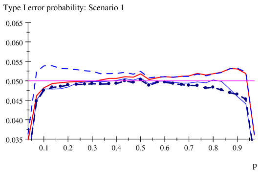
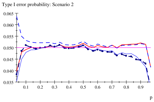
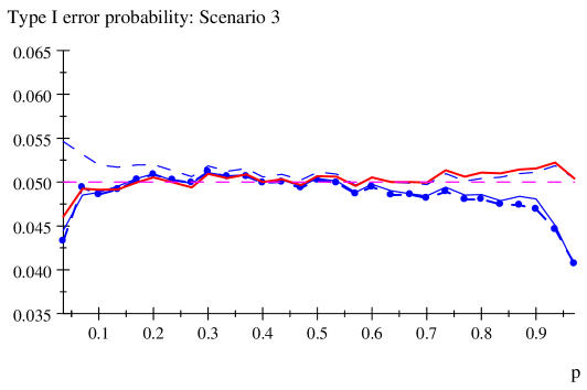
Figure 1: Exact type I error for one-sided test of trends in probabilities.

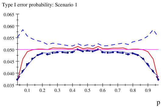
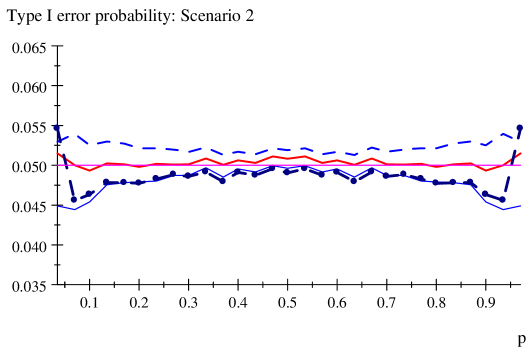
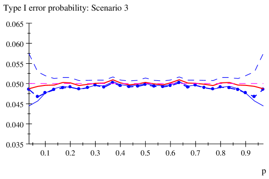
Figure 2: Exact type I error for two-sided test of trends in probabilities.

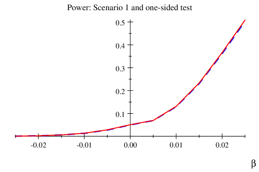
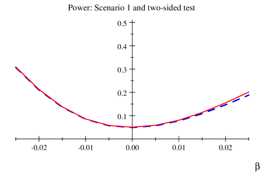
Figure 3: Exact power for one sided and two sided tests of trends in probabilities.

Appendix A Appendix: Proof of Theorem 1

In Dardanoni and Forcina [22] generalized models with linear constraints were used as tool for unifying different kind of order restricted probabilities when there is no an underlying model. By following a similar idea, using a saturated loglinear model and in addition, the case of a unique multi-sample in Martín and Balakrishnan [20], it is possible to get the result we need by considering three models, the saturated model (nonparametric), linear logit model (adding constraints on the nonparametric model) and independence model (the loglinear model without interaction parameter ). The estimated probabilities of these three models are going to be $\widehat{\boldsymbol{p}}$, $\boldsymbol{p}(\widehat{\alpha},\widehat{\beta})$, $\boldsymbol{p}(\widehat{\alpha},0)$ respectively. Since $\log\frac{p_{i1}(\alpha,\beta)}{p_{i2}(\alpha,\beta)}=\log\frac{\pi_{i1}(\alpha,\beta)}{\pi_{i2}(\alpha,\beta)}$, we can express the linear logit model either for the joint probabilities or conditional probabilities but we shall focus on joint probabilities

$$\log\frac{p_{i1}(\alpha,\beta)}{p_{i2}(\alpha,\beta)}=\alpha+\beta x_{i}.$$

The joint probabilities in terms of a saturated loglinear model are given by

$$\log p_{i1}(\alpha,\beta) =\theta_{1(i)}+\theta_{2(1)}+\theta_{12(i1)},$$

$$\log p_{i2}(\alpha,\beta) =\theta_{1(i)},$$

where we have considered the constraints $\theta_{2(2)}=\theta_{12(i2)}=0$ to avoid overparametrization and without any loss of generality we shall consider $\theta_{12(I1)}=\frac{x_{I}}{x_{1}}\theta_{12(11)}$. Once we get the values of $\alpha,\beta$, the terms $\theta_{1(i)}$, $i=1,...,I$, are calculated taking into account $p_{i1}(\alpha,\beta)+p_{i2}(\alpha,\beta)=\frac{n_{i}}{n}$, $i=1,...,I$. If we take the ratio of both logarithm of probabilities we have

$$\log\frac{p_{i1}(\alpha,\beta)}{p_{i2}(\alpha,\beta)}=\theta_{2(1)}+\theta_{12(i1)},$$

which means that $\theta_{2(1)}=\alpha$, $\theta_{12(i1)}=\beta x_{i}$, and thus the linear logit model can be reparametrized as a saturated loglinear model subject to the linear constraint

$$x_{1}\theta_{12(i1)}-x_{i}\theta_{12(11)}=0,\quad i=2,...,I-1$$ (15)

(the equation is also true for $i=I$ but it was true for the saturated model). In matrix notation the saturated loglinear model is given by

$$\log\boldsymbol{p}(\boldsymbol{\theta})=\boldsymbol{W}_{1}\boldsymbol{\theta}_{1}+\boldsymbol{W}_{12}\boldsymbol{\theta}_{12}+\boldsymbol{w}_{2}\theta_{2(1)}=\boldsymbol{W}_{1}\boldsymbol{\theta}_{1}+\boldsymbol{W\theta},$$

where $\boldsymbol{\theta}_{1}=(\theta_{1(1)},...,\theta_{1(I-1)})^{T}$, $\boldsymbol{\theta}_{12}=(\theta_{12(11)},...,\theta_{12(I-1,1)})^{T}$, $\boldsymbol{\theta}=(\boldsymbol{\theta}_{12}^{T},\theta_{2(1)})^{T}$,

$$\boldsymbol{W}_{1}=\boldsymbol{I}_{I}\otimes\boldsymbol{1}_{2},\quad\boldsymbol{W}_{12}=\begin{pmatrix}\boldsymbol{I}_{I-1}\\ \frac{x_{I}}{x_{1}}\boldsymbol{e}_{1}^{T}\end{pmatrix}\otimes\begin{pmatrix}1\\ 0\end{pmatrix},\quad\boldsymbol{w}_{2}=\boldsymbol{1}_{I}\otimes\begin{pmatrix}1\\ 0\end{pmatrix},\quad\boldsymbol{W}=(\boldsymbol{W}_{12},\boldsymbol{w}_{2}),$$

$\otimes$ is the Kronecker product (see Chapter 16 of Harville [23]), $\boldsymbol{I}_{a}$ is the the identity matrix of order $a$, $\boldsymbol{e}_{i}$ is the vector of zeros and $1$ in the $i$-th position and $\theta_{1(i)}=\log(\frac{n_{i}}{n})-\log(\boldsymbol{1}_{2}^{T}\exp\{(\boldsymbol{I}_{2}\otimes\boldsymbol{e}_{i}^{T})\boldsymbol{W\theta}\})$. The last expression is similar to the formula for getting the intercept in a product-multinomial sampling. Condition (15) in matrix notation is given by $(x_{1}\boldsymbol{1}_{I-2},-diag\{x_{i}\}_{i=2}^{I-1},\boldsymbol{0}_{I-2})\boldsymbol{\theta}=\boldsymbol{0}_{I-2}$. In this framework, for the linear logit model, (6) is equal to

$$H_{0} :\theta_{12(11)}=0\text{, }x_{1}\theta_{12(i1)}-x_{i}\theta_{12(11)}=0,\quad i=2,...,I-1,$$

$$H_{1} :\theta_{12(11)}>0\text{, }x_{1}\theta_{12(i1)}-x_{i}\theta_{12(11)}=0,\quad i=2,...,I-1,$$

for the saturated loglinear model. For the one-sided test we have three parametric spaces

$$\Omega(E) =\{\boldsymbol{\theta}\in\mathbb{R}^{I}:\boldsymbol{e}_{1}^{T}\boldsymbol{\theta}\leq 0,\quad(x_{1}\boldsymbol{1}_{I-2},-diag\{x_{i}\}_{i=2}^{I-1},\boldsymbol{0}_{I-2})\boldsymbol{\theta}=\boldsymbol{0}_{I-2}\},$$

$$\Theta(F) =\{\boldsymbol{\theta}\in\mathbb{R}^{I}:(x_{1}\boldsymbol{1}_{I-2},-diag\{x_{i}\}_{i=2}^{I-1},\boldsymbol{0}_{I-2})\boldsymbol{\theta}=\boldsymbol{0}_{I-2}\},$$

$$\Theta =\Theta(\varnothing)=\mathbb{R}^{I},$$

such that $\Theta(E)\subset\Omega(F)\subset\Theta$, this statistical problem can be placed in the nesting framework of the paper Martín and Balakrishnan [20]. In terms of the hypothesis testing formulation given in Martín and Balakrishnan [20, Section 2], the one sided hypothesis testing $H_{0}$: $\boldsymbol{\theta}\in\Omega(E)$ vs. $H_{1}$: $\boldsymbol{\theta}\in\Theta(F)-\Omega(E)$ is (12), the set of indices that the restriction is active is the same for for the null and alternative hypothesis, $E=F=\{i\in\{2,...,I-1\}:h_{i}(\boldsymbol{\theta})=0\}$, with $h_{i}(\boldsymbol{\theta})=x_{1}\theta_{12(i1)}-x_{i}\theta_{12(11)}$, $i=2,...,I-1$. The LR test match formula (20) in Martín and Balakrishnan [20, Section 2] and this is a particular test-statistics of the second test-statistic given in Definition 16 for which the same idea of (54) in the simulation study is used. Hence, the asymptotic distribution for one-sided test (6) is obtained from Theorem 17 in Martín and Balakrishnan [20, Section 2]. The maximum number of positions in parameter $\beta$ where $\beta=0$ is reached, is $1$ (if $\widehat{\beta}>0$, then $\widetilde{\beta}=0$), which means that the chi-bar square distribution of test (6) has two summands with weights equals $\frac{1}{2}$. For the two-sided test we have three parametric spaces

$$\Theta(E^{\prime}) =\{\boldsymbol{\theta}\in\mathbb{R}^{I}:\boldsymbol{e}_{1}^{T}\boldsymbol{\theta}=0,\quad(x_{1}\boldsymbol{1}_{I-2},-diag\{x_{i}\}_{i=2}^{I-1},\boldsymbol{0}_{I-2})\boldsymbol{\theta}=\boldsymbol{0}_{I-2}\},$$

$$\Theta(F^{\prime}) =\{\boldsymbol{\theta}\in\mathbb{R}^{I}:(x_{1}\boldsymbol{1}_{I-2},-diag\{x_{i}\}_{i=2}^{I-1},\boldsymbol{0}_{I-2})\boldsymbol{\theta}=\boldsymbol{0}_{I-2}\},$$

$$\Theta =\Theta(\varnothing)=\mathbb{R}^{I},$$

such that $\Theta(E^{\prime})\subset\Theta(F^{\prime})\subset\Theta$, this statistical problem can be placed in the nesting framework of the paper Martín and Balakrishnan [20]. In terms of the hypothesis testing formulation given in Martín and Balakrishnan [20, Section 2], the two sided hypothesis testing $H_{0}^{\prime}$: $\boldsymbol{\theta}\in\Theta(E^{\prime})$ vs. $H_{1}^{\prime}$: $\boldsymbol{\theta}\in\Theta(F^{\prime})-\Theta(E^{\prime})$ is (10), the set of indices that the restriction is active for the null hypothesis is $E^{\prime}=\{i\in\{1,2,...,I-1\}:h_{i}(\boldsymbol{\theta})=0\}$, with $h_{1}(\boldsymbol{\theta})=\boldsymbol{e}_{1}^{T}\boldsymbol{\theta}$, $h_{i}(\boldsymbol{\theta})=x_{1}\theta_{12(i1)}-x_{i}\theta_{12(11)}$, $i=2,...,I-1$, and $F^{\prime}=F$ for the alternative hypothesis. The LR test match formula (18) in Martín and Balakrishnan [20, Section 2] and this is a particular test-statistics of the second test-statistic given in Definition 7. Hence, the asymptotic distribution for two-sided test (8) is obtained from Theorem 8 in Martín and Balakrishnan [20, Section 2]. Note that $\mathrm{card}(E^{\prime})-\mathrm{card}(F^{\prime})=1$, which means that the chi-square distribution of (8) has one degree of freedom.

Appendix B Appendix: Proof of Theorem 2

We can follow the same idea of the previous proof. The asymptotic distributions is obtained from Theorem 8 in Martín and Balakrishnan [20, Section 2]. The parametric spaces are

$$\Theta(E^{\prime\prime}) =\{\boldsymbol{\theta}\in\mathbb{R}^{I}:(x_{1}\boldsymbol{1}_{I-2},-diag\{x_{i}\}_{i=2}^{I-1},\boldsymbol{0}_{I-2})\boldsymbol{\theta}=\boldsymbol{0}_{I-2}\},$$

$$\Theta(F^{\prime\prime}) =\Theta=\Theta(\varnothing)=\mathbb{R}^{I},$$

such that $\Theta(E^{\prime\prime})\subset\Theta(F^{\prime\prime})=\Theta$. In terms of the hypothesis testing formulation given in Martín and Balakrishnan [20, Section 2], the goodness of fit hypothesis testing $H_{0}$: $\boldsymbol{\theta}\in\Theta(E^{\prime\prime})$ vs. $H_{1}$: $\boldsymbol{\theta}\in\Theta(F^{\prime\prime})-\Theta(E^{\prime\prime})$ is (10), the set of indices that the restriction is active for the null hypothesis is $E^{\prime\prime}=E=F$ and $F^{\prime\prime}=\varnothing$ (the saturated model does not considers constraints) for the alternative hypothesis. The LR test match formula (18) in Martín and Balakrishnan [20, Section 2] and this is a particular test-statistics of the second test-statistic given in Definition 7. Hence, the asymptotic distribution for two-sided test (8) is obtained from Theorem 8 in Martín and Balakrishnan [20, Section 2]. Note that $\mathrm{card}(E^{\prime\prime})-\mathrm{card}(F^{\prime\prime})=I-2$, which means that the chi-square distribution has $I-2$ degrees of freedom under the hypothesis that the linear logit model is true.

References

• [1] Cochran WG. Some Methods for Strengthening the Common $\chi^{2}$ Tests. Biometrics 1954; 10: 417-451.
• [2] Armitage P. Tests for Linear Trends in Proportions and Frequencies. Biometrics 1955; 11: 375-386.
• [3] Mantel N. Chi-square Tests with one degree of freedom extensions of the mantel-Haenszel procedure. Journal of the American Statistical Association 1963; 58: 690-700.
• [4] Tarone RE and Gart JJ. On the Robustness of Combined Test for Trends in Proportions. Journal of the American Statistical Association, 1980; 75: 110-116.
• [5] Rao CR. Linear Statistical Inference and Its Applications. New York: Wiley, 1973.
• [6] Cox DR. Analysis of Binary Data. London: Methuen, 1970.
• [7] Cox DR. Note on Grouping. Journal of the American Statistical Association 1957; 52: 543-547.
• [8] Barlow RE, Bartholomew DJ, Bremmer JM and Brunk, HD. Statistical Inference Under Order Restrictions. New York: John Wiley & Sons, 1972.
• [9] Robertson T, Wright FT and Dykstra RL. Order Restricted Statistical Inference. New York:John Wiley & Sons, 1988.
• [10] Silvapulle MJ and Sen PK. Constrained Statistical Inference: Order, Inequality, and Shape Constraints. New York: Wiley Series in Probability and Statistics, 2004.
• [11] Leuraud K and Benichou J. A comparison of several methods to test for the existence of a monotonic dose-response relationship in clinical and epidemiological studies. Statistics in Medicine 2001; 20: 3335-3351.
• [12] Agresti A and Coull BA. An empirical comparison of inference using a order-restricted and linear logit models for a binary response. Communications in Statistics (Simulation) 1998; 27: 147-166.
• [13] Hirji KF and Tang ML. A comparison of Tests for Trend. Communications in Statistics (Theory and Methods) 1998; 27: 943-963.
• [14] Tang ML, Chan PS and Chan W. On Exact Unconditional Test for Linear Trend in Dose-Response Studies. Biometrical Journal 2000; 42: 795-806.
• [15] Shan G, Ma C. and Wilding GE. An Efficient and Exact Approach for Detecting Trends with Binary Endpoints. Statistics in Medicine 2012; 31: 155-164.
• [16] Kang S and Lee J. The size of the Cochran-Armitage trend test in 2xC contingency tables. Journal of Statistical Planning and Inference 2007; 137: 1851-1861.
• [17] Pardo, L. Statistical Inference Based on Divergence Measures. New York: Chapman & Hall/CRC, 2006.
• [18] Cressie N and Read TRC: Multinomial goodness-of-fit tests. Journal of the Royal Statistical Society, Series B 1984; 46:440-464.
• [19] Tebbs JM and Bilder CR. Hypotesis Tests for and against a Simple Order among Proportions Estimated by Pooled Testing. Biometrical Journal 2006; 48: 792-804.
• [20] Martรญn N and Balakrishnan N. Hypothesis testing in a generic nesting framework with general population distributions. Journal of Multivariate Analysis 2013; 118: 1-23.
• [21] Paris C, Thierry S, Brochard P, Letourneux M, Schorle E, Stoufflet A, Ameille J, Conso F and Pairon JC. Pleural plaques and asbestosis: dose- and time-response relationships based on HRCT data. European Respiratory Journal 2009; 34: 72-79.
• [22] Dardanoni V and Forcina A. A Unified Approach to Likelihood Inference on Stochastic Orderings in a Nonparametric Context. Journal of the American Statistical Association 1998; 93: 1112-1122.
• [23] Harville DA. Matrix Algebra From a Statisticianโ€™s Perspective. New York: Springer, 2008.