1 Introduction
Ordinal categorical data appear frequently in the biomedical research
literature, for example, in the analysis of I 𝐼 I
Table 1: Number of individuals with (j=1) and without (j=0) congenital sex-organ malformation cross-classified according to the maternal alcohol consumption level (i=1,2,3,4).
Table 1 I = 4 𝐼 4 I=4 i = 1 𝑖 1 i=1 i = 2 𝑖 2 i=2 i = 3 𝑖 3 i=3 i = 4 𝑖 4 i=4 n i subscript 𝑛 𝑖 n_{i} 1 j = 2 𝑗 2 j=2 1 j = 1 𝑗 1 j=1 1 π i subscript 𝜋 𝑖 \pi_{i} i 𝑖 i
1.
Is there any evidence of maternal alcohol consumption being related to
malformation of sex organ? To answer this question, the null and alternative
hypotheses may be formulated as
H 0 : π 1 = π 2 = π 3 = π 4 vs. H 1 : π 1 , π 2 , π 3 , π 4 are not all equal, : subscript 𝐻 0 subscript 𝜋 1 subscript 𝜋 2 subscript 𝜋 3 subscript 𝜋 4 vs. subscript 𝐻 1 : subscript 𝜋 1 subscript 𝜋 2 subscript 𝜋 3 subscript 𝜋 4 are not all equal,
H_{0}:\pi_{1}=\pi_{2}=\pi_{3}=\pi_{4}\text{ vs. }H_{1}:\pi_{1},\pi_{2},\pi_{3},\pi_{4}\text{ are not all equal,}
respectively. However, this formulation is unlikely to be appropriate because
the main issue of interest is the possible increase in the probability of
malformation as alcohol consumption increases.
2.
Is there any evidence that an increase in maternal alcohol consumption
is associated with an increase in the probability of malformation?. This
question, as it stands, is quite broad to give a precise formulation of the
null and the alternative hypotheses. One possibility is to formulate the
problem in the following way,
H 0 : π 1 = π 2 = π 3 = π 4 vs. H 1 : π 1 ≤ π 2 ≤ π 3 ≤ π 4 with at least one inequality being strict. : subscript 𝐻 0 subscript 𝜋 1 subscript 𝜋 2 subscript 𝜋 3 subscript 𝜋 4 vs. subscript 𝐻 1 : subscript 𝜋 1 subscript 𝜋 2 subscript 𝜋 3 subscript 𝜋 4 with at least one inequality being strict. H_{0}:\pi_{1}=\pi_{2}=\pi_{3}=\pi_{4}\text{ vs. }H_{1}:\pi_{1}\leq\pi_{2}\leq\pi_{3}\leq\pi_{4}\text{ with at least one inequality being strict.} (1)
Consider an experiment with I 𝐼 I X 𝑋 X n i subscript 𝑛 𝑖 n_{i} i 𝑖 i n = ∑ i = 1 I n i 𝑛 superscript subscript 𝑖 1 𝐼 subscript 𝑛 𝑖 n=\sum_{i=1}^{I}n_{i} Y 𝑌 Y N i 1 subscript 𝑁 𝑖 1 N_{i1} Y = 1 𝑌 1 Y=1 i 𝑖 i n i subscript 𝑛 𝑖 n_{i} i = 1 , … , I . 𝑖 1 … 𝐼
i=1,...,I. π i = Pr ( Y = 1 | X = i ) subscript 𝜋 𝑖 Pr 𝑌 conditional 1 𝑋 𝑖 \pi_{i}=\Pr(Y=1|X=i) i 𝑖 i N i 1 subscript 𝑁 𝑖 1 N_{i1} n i subscript 𝑛 𝑖 n_{i} π i subscript 𝜋 𝑖 \pi_{i} i = 1 , … , I 𝑖 1 … 𝐼
i=1,...,I N i 2 subscript 𝑁 𝑖 2 N_{i2} i 𝑖 i N i 2 = n i − N i 1 subscript 𝑁 𝑖 2 subscript 𝑛 𝑖 subscript 𝑁 𝑖 1 N_{i2}=n_{i}-N_{i1} ( N i 1 , N i 2 ) subscript 𝑁 𝑖 1 subscript 𝑁 𝑖 2 (N_{i1},N_{i2}) i = 1 , … , I 𝑖 1 … 𝐼
i=1,...,I
. fragments n 1 fragments n 11 fragments n 12 n 1 n 11 ⋮ ⋮ ⋮ fragments n 𝑖 fragments n 𝑖 1 fragments n 𝑖 2 n 𝑖 n 𝑖 1 ⋮ ⋮ ⋮ fragments n 𝐼 fragments n 𝐼 1 fragments n 𝐼 2 n 𝐼 n 𝐼 1 \begin{tabular}[c]{||c||cc||}\hline\cr\hline\cr$n_{1}$&$n_{11}$&$n_{12}=n_{1}-n_{11}$\\
$\vdots$&$\vdots$&$\vdots$\\
$n_{i}$&$n_{i1}$&$n_{i2}=n_{i}-n_{i1}$\\
$\vdots$&$\vdots$&$\vdots$\\
$n_{I}$&$n_{I1}$&$n_{I2}=n_{I}-n_{I1}$\\
\hline\cr\hline\cr\end{tabular}\ .
Our purpose in this paper is to propose new order-restricted test statistics,
Wald-type and phi-divergence based test-statistics for testing
H 0 subscript 𝐻 0 \displaystyle H_{0} : π 1 = π 2 = ⋯ = π I , : absent subscript 𝜋 1 subscript 𝜋 2 ⋯ subscript 𝜋 𝐼 \displaystyle:\pi_{1}=\pi_{2}=\cdots=\pi_{I}, (2)
H 1 subscript 𝐻 1 \displaystyle H_{1} : π 1 ≤ π 2 ≤ ⋯ ≤ π I with at least one
inequality being strict. : absent subscript 𝜋 1 subscript 𝜋 2 ⋯ subscript 𝜋 𝐼 with at least one
inequality being strict. \displaystyle:\pi_{1}\leq\pi_{2}\leq\cdots\leq\pi_{I}\text{ with at least one
inequality being strict.}
The classical likelihood ratio test statistic will appear as a particular case
of phi-divergence based test-statistics. A log-linear formulation of
(1 2 3 4 1 5
2 Formulation for isotonic binomial proportions in terms of log-linear
and logistic regression modeling: Wald type test-statistics
Reparametrizating the initial problem through log-linear modeling, the
formulation of the null hypothesis is strongly simplified since all the
interaction parameters are zero under the null hypothesis and this is
appealing, in special, to create Wald type test-statistics. Let
𝒑 𝒑 \displaystyle\boldsymbol{p} = 𝒑 ( 𝜽 ) = ( p 11 ( 𝜽 ) , p 12 ( 𝜽 ) , p 21 ( 𝜽 ) , p 22 ( 𝜽 ) , … , p I 1 ( 𝜽 ) , p I 2 ( 𝜽 ) ) T absent 𝒑 𝜽 superscript subscript 𝑝 11 𝜽 subscript 𝑝 12 𝜽 subscript 𝑝 21 𝜽 subscript 𝑝 22 𝜽 … subscript 𝑝 𝐼 1 𝜽 subscript 𝑝 𝐼 2 𝜽 𝑇 \displaystyle=\boldsymbol{p}(\boldsymbol{\theta})=(p_{11}(\boldsymbol{\theta}),p_{12}(\boldsymbol{\theta}),p_{21}(\boldsymbol{\theta}),p_{22}(\boldsymbol{\theta}),...,p_{I1}(\boldsymbol{\theta}),p_{I2}(\boldsymbol{\theta}))^{T}
= ( n 1 n π 1 , n 1 n ( 1 − π 1 ) , n 2 n π 2 , n 2 n ( 1 − π 2 ) , … , n I n π I , n I n ( 1 − π I ) ) T absent superscript subscript 𝑛 1 𝑛 subscript 𝜋 1 subscript 𝑛 1 𝑛 1 subscript 𝜋 1 subscript 𝑛 2 𝑛 subscript 𝜋 2 subscript 𝑛 2 𝑛 1 subscript 𝜋 2 … subscript 𝑛 𝐼 𝑛 subscript 𝜋 𝐼 subscript 𝑛 𝐼 𝑛 1 subscript 𝜋 𝐼 𝑇 \displaystyle=(\tfrac{n_{1}}{n}\pi_{1},\tfrac{n_{1}}{n}(1-\pi_{1}),\tfrac{n_{2}}{n}\pi_{2},\tfrac{n_{2}}{n}(1-\pi_{2}),...,\tfrac{n_{I}}{n}\pi_{I},\tfrac{n_{I}}{n}(1-\pi_{I}))^{T} (3)
be the probability vector of the following saturated log-linear model
log p i j ( 𝜽 ) = u + u 1 ( i ) + θ 2 ( j ) + θ 12 ( i j ) , subscript 𝑝 𝑖 𝑗 𝜽 𝑢 subscript 𝑢 1 𝑖 subscript 𝜃 2 𝑗 subscript 𝜃 12 𝑖 𝑗 \log p_{ij}(\boldsymbol{\theta})=u+u_{1(i)}+\theta_{2(j)}+\theta_{12(ij)}, (4)
with
u 1 ( I ) = 0 , θ 2 ( 2 ) = 0 , θ 12 ( i 2 ) = 0 , i = 1 , … , I − 1 , θ 12 ( I j ) = 0 , j = 1 , 2 , formulae-sequence subscript 𝑢 1 𝐼 0 formulae-sequence subscript 𝜃 2 2 0 formulae-sequence subscript 𝜃 12 𝑖 2 0 formulae-sequence 𝑖 1 … 𝐼 1
formulae-sequence subscript 𝜃 12 𝐼 𝑗 0 𝑗 1 2
u_{1(I)}=0,\quad\theta_{2(2)}=0,\quad\theta_{12(i2)}=0,i=1,...,I-1,\quad\theta_{12(Ij)}=0,j=1,2, (5)
being the identifiability constraints,
𝜽 = ( θ 2 ( 1 ) , θ 12 ( 11 ) , … , θ 12 ( 1 I − 1 ) ) T 𝜽 superscript subscript 𝜃 2 1 subscript 𝜃 12 11 … subscript 𝜃 12 1 𝐼 1 𝑇 \boldsymbol{\theta}=(\theta_{2(1)},\theta_{12(11)},...,\theta_{12(1I-1)})^{T} (6)
the unknown parameters vector and 𝒖 = ( u , u 1 ( 1 ) , … , u 1 ( I − 1 ) ) T 𝒖 superscript 𝑢 subscript 𝑢 1 1 … subscript 𝑢 1 𝐼 1 𝑇 \boldsymbol{u}=(u,u_{1(1)},...,u_{1(I-1)})^{T}
u = u ( 𝜽 ) = log n I / n 1 + exp { θ 2 ( 1 ) } , 𝑢 𝑢 𝜽 subscript 𝑛 𝐼 𝑛 1 subscript 𝜃 2 1 u=u(\boldsymbol{\theta})=\log\frac{n_{I}/n}{1+\exp\{\theta_{2(1)}\}}, (7)
u 1 ( i ) = u 1 ( i ) ( 𝜽 ) = log n i n I ( 1 + exp { θ 2 ( 1 ) } ) 1 + exp { θ 2 ( 1 ) + θ 12 ( i 1 ) } , i = 1 , … , I − 1 , formulae-sequence subscript 𝑢 1 𝑖 subscript 𝑢 1 𝑖 𝜽 subscript 𝑛 𝑖 subscript 𝑛 𝐼 1 subscript 𝜃 2 1 1 subscript 𝜃 2 1 subscript 𝜃 12 𝑖 1 𝑖 1 … 𝐼 1
u_{1(i)}=u_{1(i)}(\boldsymbol{\theta})=\log\frac{\frac{n_{i}}{n_{I}}\left(1+\exp\{\theta_{2(1)}\}\right)}{1+\exp\{\theta_{2(1)}+\theta_{12(i1)}\}},\quad i=1,...,I-1, (8)
the redundant parameters, obtained through 𝜽 𝜽 \boldsymbol{\theta} p i 1 ( 𝜽 ) + p i 0 ( 𝜽 ) = n i n subscript 𝑝 𝑖 1 𝜽 subscript 𝑝 𝑖 0 𝜽 subscript 𝑛 𝑖 𝑛 p_{i1}(\boldsymbol{\theta})+p_{i0}(\boldsymbol{\theta})=\frac{n_{i}}{n} i = 1 , … , I 𝑖 1 … 𝐼
i=1,...,I 2
H 0 subscript 𝐻 0 \displaystyle H_{0} : θ 12 ( 11 ) = θ 12 ( 21 ) = ⋯ = θ 12 ( I − 1 , 1 ) = 0 , : absent subscript 𝜃 12 11 subscript 𝜃 12 21 ⋯ subscript 𝜃 12 𝐼 1 1 0 \displaystyle:\theta_{12(11)}=\theta_{12(21)}=\cdots=\theta_{12(I-1,1)}=0, (9)
H 1 subscript 𝐻 1 \displaystyle H_{1} : θ 12 ( 11 ) ≤ θ 12 ( 21 ) ≤ ⋯ ≤ θ 12 ( I − 1 , 1 ) ≤ 0 with at least one inequality being strict. : absent subscript 𝜃 12 11 subscript 𝜃 12 21 ⋯ subscript 𝜃 12 𝐼 1 1 0 with at least one inequality being strict. \displaystyle:\theta_{12(11)}\leq\theta_{12(21)}\leq\cdots\leq\theta_{12(I-1,1)}\leq 0\text{ with at least one inequality being strict.}
Notice that θ 2 ( 1 ) subscript 𝜃 2 1 \theta_{2(1)} 9 π 0 = π 1 = π 2 = ⋯ = π I subscript 𝜋 0 subscript 𝜋 1 subscript 𝜋 2 ⋯ subscript 𝜋 𝐼 \pi_{0}=\pi_{1}=\pi_{2}=\cdots=\pi_{I} θ 2 ( 1 ) = logit ( π 0 ) = log [ π 0 / ( 1 − π 0 ) ] subscript 𝜃 2 1 logit subscript 𝜋 0 subscript 𝜋 0 1 subscript 𝜋 0 \theta_{2(1)}=\mathrm{logit}(\pi_{0})=\log[\pi_{0}/(1-\pi_{0})]
In matrix notation, we can express the vector of parameters of the log-linear
model in terms of the following logistic regression
logit ( 𝝅 ) = 𝑿 𝜽 logit 𝝅 𝑿 𝜽 \mathrm{logit}(\boldsymbol{\pi})=\boldsymbol{X\theta} (10)
where
𝝅 = ( π 1 , π 2 , … , π I ) T , 𝑿 = ( 𝟏 I − 1 𝑰 I − 1 1 𝟎 I − 1 T ) , formulae-sequence 𝝅 superscript subscript 𝜋 1 subscript 𝜋 2 … subscript 𝜋 𝐼 𝑇 𝑿 matrix subscript 1 𝐼 1 subscript 𝑰 𝐼 1 1 superscript subscript 0 𝐼 1 𝑇 \boldsymbol{\pi}=(\pi_{1},\pi_{2},...,\pi_{I})^{T},\qquad\boldsymbol{X}=\begin{pmatrix}\boldsymbol{1}_{I-1}&\boldsymbol{I}_{I-1}\\
1&\boldsymbol{0}_{I-1}^{T}\end{pmatrix},
𝑰 a subscript 𝑰 𝑎 \boldsymbol{I}_{a} a 𝑎 a 𝟏 a subscript 1 𝑎 \boldsymbol{1}_{a} a 𝑎 a 𝟎 a subscript 0 𝑎 \boldsymbol{0}_{a} a 𝑎 a 𝑿 𝑿 \boldsymbol{X}
𝜽 = 𝑿 − 1 logit ( 𝝅 ) , 𝜽 superscript 𝑿 1 logit 𝝅 \boldsymbol{\theta}=\boldsymbol{X}^{-1}\mathrm{logit}(\boldsymbol{\pi}), (11)
and on the other hand (9
H 0 subscript 𝐻 0 \displaystyle H_{0} : 𝑹 𝜽 = 𝟎 I − 1 , : absent 𝑹 𝜽 subscript 0 𝐼 1 \displaystyle:\boldsymbol{R\theta}=\boldsymbol{0}_{I-1}, (12)
H 1 subscript 𝐻 1 \displaystyle H_{1} : 𝑹 𝜽 ≤ 𝟎 I − 1 and 𝑹 𝜽 ≠ 𝟎 I − 1 , : absent 𝑹 𝜽 subscript 0 𝐼 1 and 𝑹 𝜽 subscript 0 𝐼 1 , \displaystyle:\boldsymbol{R\theta}\leq\boldsymbol{0}_{I-1}\text{ and
}\boldsymbol{R\theta}\neq\boldsymbol{0}_{I-1}\text{,}
with 𝑹 = ( 𝟎 I − 1 , 𝑮 I − 1 ) 𝑹 subscript 0 𝐼 1 subscript 𝑮 𝐼 1 \boldsymbol{R}=(\boldsymbol{0}_{I-1},\boldsymbol{G}_{I-1}) 𝑮 I − 1 subscript 𝑮 𝐼 1 \boldsymbol{G}_{I-1} I − 1 𝐼 1 I-1 1 1 1 − 1 1 -1
We shall consider three parameter spaces for 𝜽 𝜽 \boldsymbol{\theta}
Θ 0 = { 𝜽 ∈ ℝ I : 𝑹 𝜽 = 𝟎 I − 1 } ⊂ Θ ~ = { 𝜽 ∈ ℝ I : 𝑹 𝜽 ≤ 𝟎 I − 1 } ⊂ Θ = ℝ I , subscript Θ 0 conditional-set 𝜽 superscript ℝ 𝐼 𝑹 𝜽 subscript 0 𝐼 1 ~ Θ conditional-set 𝜽 superscript ℝ 𝐼 𝑹 𝜽 subscript 0 𝐼 1 Θ superscript ℝ 𝐼 \Theta_{0}=\left\{\boldsymbol{\theta}\in\mathbb{R}^{I}:\boldsymbol{R\theta}=\boldsymbol{0}_{I-1}\right\}\subset\widetilde{\Theta}=\left\{\boldsymbol{\theta}\in\mathbb{R}^{I}:\boldsymbol{R\theta}\leq\boldsymbol{0}_{I-1}\right\}\subset\Theta=\mathbb{R}^{I},
i.e. while Θ Θ \Theta Θ ¯ ¯ Θ \bar{\Theta} Θ 0 subscript Θ 0 \Theta_{0} 𝜽 ∈ Θ 𝜽 Θ \boldsymbol{\theta}\in\Theta
ℐ F ( 𝜽 ) = 𝑿 T diag { ν i π i ( 1 − π i ) } i = 1 I 𝑿 , subscript ℐ 𝐹 𝜽 superscript 𝑿 𝑇 diag superscript subscript subscript 𝜈 𝑖 subscript 𝜋 𝑖 1 subscript 𝜋 𝑖 𝑖 1 𝐼 𝑿 \mathcal{I}_{F}(\boldsymbol{\theta})=\boldsymbol{X}^{T}\mathrm{diag}\{\nu_{i}\pi_{i}(1-\pi_{i})\}_{i=1}^{I}\boldsymbol{X}, (13)
where ν i = lim n → ∞ n i n subscript 𝜈 𝑖 subscript → 𝑛 subscript 𝑛 𝑖 𝑛 \nu_{i}=\lim_{n\rightarrow\infty}\frac{n_{i}}{n} i = 1 , … , I 𝑖 1 … 𝐼
i=1,...,I 2 9
Theorem 1
For 𝛉 0 ∈ Θ 0 subscript 𝛉 0 subscript Θ 0 \boldsymbol{\theta}_{0}\in\Theta_{0} 4 10
ℐ F ( 𝜽 ^ ) = π 0 ( 1 − π 0 ) ( 1 ν 1 ν 2 ⋯ ν I − 1 ν 1 ν 1 0 ⋯ 0 ν 2 0 ν 2 0 ⋮ ⋮ ⋱ ⋮ ν I − 1 0 0 ⋯ ν I − 1 ) . subscript ℐ 𝐹 ^ 𝜽 subscript 𝜋 0 1 subscript 𝜋 0 matrix 1 subscript 𝜈 1 subscript 𝜈 2 ⋯ subscript 𝜈 𝐼 1 subscript 𝜈 1 subscript 𝜈 1 0 ⋯ 0 subscript 𝜈 2 0 subscript 𝜈 2 missing-subexpression 0 ⋮ ⋮ missing-subexpression ⋱ ⋮ subscript 𝜈 𝐼 1 0 0 ⋯ subscript 𝜈 𝐼 1 \mathcal{I}_{F}(\widehat{\boldsymbol{\theta}})=\pi_{0}(1-\pi_{0})\begin{pmatrix}1&\nu_{1}&\nu_{2}&\cdots&\nu_{I-1}\\
\nu_{1}&\nu_{1}&0&\cdots&0\\
\nu_{2}&0&\nu_{2}&&0\\
\vdots&\vdots&&\ddots&\vdots\\
\nu_{I-1}&0&0&\cdots&\nu_{I-1}\end{pmatrix}. (14)
Proof. It is immediate by plugging π i = π 0 subscript 𝜋 𝑖 subscript 𝜋 0 \pi_{i}=\pi_{0} i = 1 , … , I 𝑖 1 … 𝐼
i=1,...,I 13
If 𝜽 ^ ^ 𝜽 \widehat{\boldsymbol{\theta}} 𝜽 ~ ~ 𝜽 \widetilde{\boldsymbol{\theta}} 𝜽 ¯ ¯ 𝜽 \overline{\boldsymbol{\theta}} 𝜽 𝜽 \boldsymbol{\theta} Θ 0 subscript Θ 0 \Theta_{0} Θ ~ ~ Θ \widetilde{\Theta} Θ Θ \Theta
W ( 𝜽 ~ , 𝜽 ^ ) 𝑊 ~ 𝜽 ^ 𝜽 \displaystyle W(\widetilde{\boldsymbol{\theta}},\widehat{\boldsymbol{\theta}}) = n 𝜽 ~ T 𝑹 T ( 𝑹 ℐ F − 1 ( 𝜽 ^ ) 𝑹 T ) − 1 𝑹 𝜽 ~ , absent 𝑛 superscript ~ 𝜽 𝑇 superscript 𝑹 𝑇 superscript 𝑹 superscript subscript ℐ 𝐹 1 ^ 𝜽 superscript 𝑹 𝑇 1 𝑹 ~ 𝜽 \displaystyle=n\widetilde{\boldsymbol{\theta}}^{T}\boldsymbol{R}^{T}\left(\boldsymbol{R}\mathcal{I}_{F}^{-1}(\widehat{\boldsymbol{\theta}})\boldsymbol{R}^{T}\right)^{-1}\boldsymbol{R}\widetilde{\boldsymbol{\theta}}, (15)
H ( 𝜽 ~ , 𝜽 ^ ) 𝐻 ~ 𝜽 ^ 𝜽 \displaystyle H(\widetilde{\boldsymbol{\theta}},\widehat{\boldsymbol{\theta}}) = n ( 𝜽 ~ − 𝜽 ^ ) T ℐ F ( 𝜽 ^ ) ( 𝜽 ~ − 𝜽 ^ ) , absent 𝑛 superscript ~ 𝜽 ^ 𝜽 𝑇 subscript ℐ 𝐹 ^ 𝜽 ~ 𝜽 ^ 𝜽 \displaystyle=n(\widetilde{\boldsymbol{\theta}}-\widehat{\boldsymbol{\theta}})^{T}\mathcal{I}_{F}(\widehat{\boldsymbol{\theta}})(\widetilde{\boldsymbol{\theta}}-\widehat{\boldsymbol{\theta}}), (16)
D ( 𝜽 ¯ , 𝜽 ~ , 𝜽 ^ ) 𝐷 ¯ 𝜽 ~ 𝜽 ^ 𝜽 \displaystyle D(\overline{\boldsymbol{\theta}},\widetilde{\boldsymbol{\theta}},\widehat{\boldsymbol{\theta}}) = n ( 𝜽 ¯ − 𝜽 ^ ) T ℐ F ( 𝜽 ^ ) ( 𝜽 ¯ − 𝜽 ^ ) − n ( 𝜽 ¯ − 𝜽 ~ ) T ℐ F ( 𝜽 ~ ) ( 𝜽 ¯ − 𝜽 ~ ) , absent 𝑛 superscript ¯ 𝜽 ^ 𝜽 𝑇 subscript ℐ 𝐹 ^ 𝜽 ¯ 𝜽 ^ 𝜽 𝑛 superscript ¯ 𝜽 ~ 𝜽 𝑇 subscript ℐ 𝐹 ~ 𝜽 ¯ 𝜽 ~ 𝜽 \displaystyle=n(\overline{\boldsymbol{\theta}}-\widehat{\boldsymbol{\theta}})^{T}\mathcal{I}_{F}(\widehat{\boldsymbol{\theta}})(\overline{\boldsymbol{\theta}}-\widehat{\boldsymbol{\theta}})-n(\overline{\boldsymbol{\theta}}-\widetilde{\boldsymbol{\theta}})^{T}\mathcal{I}_{F}(\widetilde{\boldsymbol{\theta}})(\overline{\boldsymbol{\theta}}-\widetilde{\boldsymbol{\theta}}), (17)
where
ℐ F ( 𝜽 ^ ) subscript ℐ 𝐹 ^ 𝜽 \displaystyle\mathcal{I}_{F}(\widehat{\boldsymbol{\theta}}) = π ^ 0 ( 1 − π ^ 0 ) ( 1 ( 𝝂 ^ ∗ ) T 𝝂 ^ ∗ diag ( 𝝂 ^ ∗ ) ) , absent subscript ^ 𝜋 0 1 subscript ^ 𝜋 0 matrix 1 superscript superscript ^ 𝝂 ∗ 𝑇 superscript ^ 𝝂 ∗ diag superscript ^ 𝝂 ∗ \displaystyle=\widehat{\pi}_{0}(1-\widehat{\pi}_{0})\begin{pmatrix}1&(\widehat{\boldsymbol{\nu}}^{\ast})^{T}\\
\widehat{\boldsymbol{\nu}}^{\ast}&\mathrm{diag}(\widehat{\boldsymbol{\nu}}^{\ast})\end{pmatrix},
ℐ F ( 𝜽 ~ ) subscript ℐ 𝐹 ~ 𝜽 \displaystyle\mathcal{I}_{F}(\widetilde{\boldsymbol{\theta}}) = 𝑿 T diag { ν ^ i π ~ i ( 1 − π ~ i ) } i = 1 I 𝑿 , absent superscript 𝑿 𝑇 diag superscript subscript subscript ^ 𝜈 𝑖 subscript ~ 𝜋 𝑖 1 subscript ~ 𝜋 𝑖 𝑖 1 𝐼 𝑿 \displaystyle=\boldsymbol{X}^{T}\mathrm{diag}\{\widehat{\nu}_{i}\widetilde{\pi}_{i}(1-\widetilde{\pi}_{i})\}_{i=1}^{I}\boldsymbol{X},
𝝂 ^ ∗ superscript ^ 𝝂 ∗ \displaystyle\widehat{\boldsymbol{\nu}}^{\ast} = ( ν ^ 1 , … , ν ^ I − 1 ) T = ( n 1 n , … , n I − 1 n ) T . absent superscript subscript ^ 𝜈 1 … subscript ^ 𝜈 𝐼 1 𝑇 superscript subscript 𝑛 1 𝑛 … subscript 𝑛 𝐼 1 𝑛 𝑇 \displaystyle=(\widehat{\nu}_{1},...,\widehat{\nu}_{I-1})^{T}=(\frac{n_{1}}{n},...,\frac{n_{I-1}}{n})^{T}.
These test-statistics, have according to Proposition 4.4.1 in Silvapulle and
Sen (2005), the same asymptotic distribution as the likelihood ratio test-statistic.
Proposition 2
Under the null hypothesis given in (2 9 W ( 𝛉 ~ , 𝛉 ^ ) 𝑊 ~ 𝛉 ^ 𝛉 W(\widetilde{\boldsymbol{\theta}},\widehat{\boldsymbol{\theta}}) 15
W ( 𝜽 ~ , 𝜽 ^ ) = n π ^ 0 ( 1 − π ^ 0 ) ( 𝜽 ~ ∗ ) T 𝚺 𝝂 ^ ∗ 𝜽 ~ ∗ , 𝑊 ~ 𝜽 ^ 𝜽 𝑛 subscript ^ 𝜋 0 1 subscript ^ 𝜋 0 superscript superscript ~ 𝜽 ∗ 𝑇 subscript 𝚺 superscript ^ 𝝂 ∗ superscript ~ 𝜽 ∗ W(\widetilde{\boldsymbol{\theta}},\widehat{\boldsymbol{\theta}})=n\widehat{\pi}_{0}(1-\widehat{\pi}_{0})(\widetilde{\boldsymbol{\theta}}^{\ast})^{T}\boldsymbol{\Sigma}_{\widehat{\boldsymbol{\nu}}^{\ast}}\widetilde{\boldsymbol{\theta}}^{\ast},
where 𝛉 ∗ = ( θ 12 ( 11 ) , … , θ 12 ( 1 I − 1 ) ) T superscript 𝛉 ∗ superscript subscript 𝜃 12 11 … subscript 𝜃 12 1 𝐼 1 𝑇 \boldsymbol{\theta}^{\ast}=(\theta_{12(11)},...,\theta_{12(1I-1)})^{T} 𝚺 𝛎 ^ ∗ = diag ( 𝛎 ^ ∗ ) − 𝛎 ^ ∗ ( 𝛎 ^ ∗ ) T subscript 𝚺 superscript ^ 𝛎 ∗ diag superscript ^ 𝛎 ∗ superscript ^ 𝛎 ∗ superscript superscript ^ 𝛎 ∗ 𝑇 \boldsymbol{\Sigma}_{\widehat{\boldsymbol{\nu}}^{\ast}}=\mathrm{diag}(\widehat{\boldsymbol{\nu}}^{\ast})-\widehat{\boldsymbol{\nu}}^{\ast}(\widehat{\boldsymbol{\nu}}^{\ast})^{T}
π ^ 0 subscript ^ 𝜋 0 \displaystyle\widehat{\pi}_{0} = N ∙ 1 n , absent subscript 𝑁 ∙ absent 1 𝑛 \displaystyle=\tfrac{N_{\bullet 1}}{n},
N ∙ 1 subscript 𝑁 ∙ absent 1 \displaystyle N_{\bullet 1} = N 11 + N 21 + … + N I 1 . absent subscript 𝑁 11 subscript 𝑁 21 … subscript 𝑁 𝐼 1 \displaystyle=N_{11}+N_{21}+...+N_{I1}.
Proof. From Theorem 1 2 × 2 2 2 2\times 2
ℐ F ( 𝜽 0 ) = π ^ 0 ( 1 − π ^ 0 ) ( 1 ( 𝝂 ^ ∗ ) T 𝝂 ^ ∗ diag ( 𝝂 ^ ∗ ) ) subscript ℐ 𝐹 subscript 𝜽 0 subscript ^ 𝜋 0 1 subscript ^ 𝜋 0 matrix 1 superscript superscript ^ 𝝂 ∗ 𝑇 superscript ^ 𝝂 ∗ diag superscript ^ 𝝂 ∗ \mathcal{I}_{F}(\boldsymbol{\theta}_{0})=\widehat{\pi}_{0}(1-\widehat{\pi}_{0})\begin{pmatrix}1&(\widehat{\boldsymbol{\nu}}^{\ast})^{T}\\
\widehat{\boldsymbol{\nu}}^{\ast}&\mathrm{diag}(\widehat{\boldsymbol{\nu}}^{\ast})\end{pmatrix}
and
ℐ F − 1 ( 𝜽 0 ) = 1 π ^ 0 ( 1 − π ^ 0 ) ( a 𝒃 T 𝒄 𝑫 ) , superscript subscript ℐ 𝐹 1 subscript 𝜽 0 1 subscript ^ 𝜋 0 1 subscript ^ 𝜋 0 matrix 𝑎 superscript 𝒃 𝑇 𝒄 𝑫 \mathcal{I}_{F}^{-1}(\boldsymbol{\theta}_{0})=\frac{1}{\widehat{\pi}_{0}(1-\widehat{\pi}_{0})}\begin{pmatrix}a&\boldsymbol{b}^{T}\\
\boldsymbol{c}&\boldsymbol{D}\end{pmatrix},
with 𝑫 = 𝚺 𝝂 ^ ∗ − 1 𝑫 superscript subscript 𝚺 superscript ^ 𝝂 ∗ 1 \boldsymbol{D}=\boldsymbol{\Sigma}_{\widehat{\boldsymbol{\nu}}^{\ast}}^{-1} 𝚺 𝝂 ^ ∗ = diag ( 𝝂 ^ ∗ ) − 𝝂 ^ ∗ ( 𝝂 ^ ∗ ) T subscript 𝚺 superscript ^ 𝝂 ∗ diag superscript ^ 𝝂 ∗ superscript ^ 𝝂 ∗ superscript superscript ^ 𝝂 ∗ 𝑇 \boldsymbol{\Sigma}_{\widehat{\boldsymbol{\nu}}^{\ast}}=\mathrm{diag}(\widehat{\boldsymbol{\nu}}^{\ast})-\widehat{\boldsymbol{\nu}}^{\ast}(\widehat{\boldsymbol{\nu}}^{\ast})^{T}
𝑹 ℐ F − 1 ( 𝜽 ^ ) 𝑹 T = 1 π ^ 0 ( 1 − π ^ 0 ) 𝑮 I − 1 𝚺 𝝂 ^ ∗ − 1 𝑮 I − 1 T 𝑹 superscript subscript ℐ 𝐹 1 ^ 𝜽 superscript 𝑹 𝑇 1 subscript ^ 𝜋 0 1 subscript ^ 𝜋 0 subscript 𝑮 𝐼 1 superscript subscript 𝚺 superscript ^ 𝝂 ∗ 1 superscript subscript 𝑮 𝐼 1 𝑇 \boldsymbol{R}\mathcal{I}_{F}^{-1}(\widehat{\boldsymbol{\theta}})\boldsymbol{R}^{T}=\frac{1}{\widehat{\pi}_{0}(1-\widehat{\pi}_{0})}\boldsymbol{G}_{I-1}\boldsymbol{\Sigma}_{\widehat{\boldsymbol{\nu}}^{\ast}}^{-1}\boldsymbol{G}_{I-1}^{T}
and
𝑹 𝜽 ~ = 𝑮 I − 1 𝜽 ∗ . 𝑹 ~ 𝜽 subscript 𝑮 𝐼 1 superscript 𝜽 ∗ \boldsymbol{R}\widetilde{\boldsymbol{\theta}}=\boldsymbol{G}_{I-1}\boldsymbol{\theta}^{\ast}.
Therefore,
W ( 𝜽 ~ , 𝜽 ^ ) 𝑊 ~ 𝜽 ^ 𝜽 \displaystyle W(\widetilde{\boldsymbol{\theta}},\widehat{\boldsymbol{\theta}}) = n 𝜽 ~ T 𝑹 T ( 𝑹 ℐ F − 1 ( 𝜽 ^ ) 𝑹 T ) − 1 𝑹 𝜽 ~ absent 𝑛 superscript ~ 𝜽 𝑇 superscript 𝑹 𝑇 superscript 𝑹 superscript subscript ℐ 𝐹 1 ^ 𝜽 superscript 𝑹 𝑇 1 𝑹 ~ 𝜽 \displaystyle=n\widetilde{\boldsymbol{\theta}}^{T}\boldsymbol{R}^{T}\left(\boldsymbol{R}\mathcal{I}_{F}^{-1}(\widehat{\boldsymbol{\theta}})\boldsymbol{R}^{T}\right)^{-1}\boldsymbol{R}\widetilde{\boldsymbol{\theta}}
= n π ^ 0 ( 1 − π ^ 0 ) ( 𝜽 ~ ∗ ) T 𝚺 𝝂 ^ ∗ 𝜽 ~ ∗ . absent 𝑛 subscript ^ 𝜋 0 1 subscript ^ 𝜋 0 superscript superscript ~ 𝜽 ∗ 𝑇 subscript 𝚺 superscript ^ 𝝂 ∗ superscript ~ 𝜽 ∗ \displaystyle=n\widehat{\pi}_{0}(1-\widehat{\pi}_{0})(\widetilde{\boldsymbol{\theta}}^{\ast})^{T}\boldsymbol{\Sigma}_{\widehat{\boldsymbol{\nu}}^{\ast}}\widetilde{\boldsymbol{\theta}}^{\ast}.
There is an explicit formula for the MLEs of 𝜽 𝜽 \boldsymbol{\theta}
𝜽 ^ = ( θ ^ 2 ( 1 ) , θ ^ 12 ( 11 ) , … , θ ^ 12 ( 1 I − 1 ) ) T = ( logit ( π ^ 0 ) , 0 , … , 0 ) T . ^ 𝜽 superscript subscript ^ 𝜃 2 1 subscript ^ 𝜃 12 11 … subscript ^ 𝜃 12 1 𝐼 1 𝑇 superscript logit subscript ^ 𝜋 0 0 … 0 𝑇 \widehat{\boldsymbol{\theta}}=(\widehat{\theta}_{2(1)},\widehat{\theta}_{12(11)},...,\widehat{\theta}_{12(1I-1)})^{T}=(\mathrm{logit}(\widehat{\pi}_{0}),0,...,0)^{T}. (18)
For the calculation of 𝜽 ~ = ( θ ~ 2 ( 1 ) , θ ~ 12 ( 11 ) , … , θ ~ 12 ( 1 I − 1 ) ) T ~ 𝜽 superscript subscript ~ 𝜃 2 1 subscript ~ 𝜃 12 11 … subscript ~ 𝜃 12 1 𝐼 1 𝑇 \widetilde{\boldsymbol{\theta}}=(\widetilde{\theta}_{2(1)},\widetilde{\theta}_{12(11)},...,\widetilde{\theta}_{12(1I-1)})^{T} 𝜽 ¯ = ( θ ¯ 2 ( 1 ) , θ ¯ 12 ( 11 ) , … , θ ¯ 12 ( 1 I − 1 ) ) T ¯ 𝜽 superscript subscript ¯ 𝜃 2 1 subscript ¯ 𝜃 12 11 … subscript ¯ 𝜃 12 1 𝐼 1 𝑇 \overline{\boldsymbol{\theta}}=(\overline{\theta}_{2(1)},\overline{\theta}_{12(11)},...,\overline{\theta}_{12(1I-1)})^{T} 𝝅 ~ = ( π ~ 1 , π ~ 2 , … , π ~ I ) T ~ 𝝅 superscript subscript ~ 𝜋 1 subscript ~ 𝜋 2 … subscript ~ 𝜋 𝐼 𝑇 \widetilde{\boldsymbol{\pi}}=(\widetilde{\pi}_{1},\widetilde{\pi}_{2},...,\widetilde{\pi}_{I})^{T} 𝝅 ¯ = ( π ¯ 1 , π ¯ 2 , … , π ¯ I ) T ¯ 𝝅 superscript subscript ¯ 𝜋 1 subscript ¯ 𝜋 2 … subscript ¯ 𝜋 𝐼 𝑇 \overline{\boldsymbol{\pi}}=(\overline{\pi}_{1},\overline{\pi}_{2},...,\overline{\pi}_{I})^{T} 11
𝝅 ¯ = ( N 11 n 1 , N 21 n 2 , … , N I 1 n I ) T , ¯ 𝝅 superscript subscript 𝑁 11 subscript 𝑛 1 subscript 𝑁 21 subscript 𝑛 2 … subscript 𝑁 𝐼 1 subscript 𝑛 𝐼 𝑇 \overline{\boldsymbol{\pi}}=(\tfrac{N_{11}}{n_{1}},\tfrac{N_{21}}{n_{2}},...,\tfrac{N_{I1}}{n_{I}})^{T}, (19)
and for calculating 𝝅 ~ ~ 𝝅 \widetilde{\boldsymbol{\pi}}
Algorithm 3 (Order restricted estimation of probabilities)
The MLE of
𝛑 = ( π 1 , π 2 , ⋯ , π I ) T 𝛑 superscript subscript 𝜋 1 subscript 𝜋 2 ⋯ subscript 𝜋 𝐼 𝑇 \boldsymbol{\pi}=(\pi_{1},\pi_{2},\cdots,\pi_{I})^{T} π 1 ≤ π 2 ≤ ⋯ ≤ π I subscript 𝜋 1 subscript 𝜋 2 ⋯ subscript 𝜋 𝐼 \pi_{1}\leq\pi_{2}\leq\cdots\leq\pi_{I} 𝛑 ~ = ( π ~ 1 , π ~ 2 , ⋯ , π ~ I ) T ~ 𝛑 superscript subscript ~ 𝜋 1 subscript ~ 𝜋 2 ⋯ subscript ~ 𝜋 𝐼 𝑇 \widetilde{\boldsymbol{\pi}}=(\widetilde{\pi}_{1},\widetilde{\pi}_{2},\cdots,\widetilde{\pi}_{I})^{T}
STEP 1: Do 𝛑 ~ := 𝛑 ¯ assign ~ 𝛑 ¯ 𝛑 \widetilde{\boldsymbol{\pi}}:=\overline{\boldsymbol{\pi}} 𝛑 ¯ ¯ 𝛑 \overline{\boldsymbol{\pi}} is
( 19 ) .
π ~ i ≤ π ~ i + 1 subscript ~ π i subscript ~ π i 1 \widetilde{\pi}_{i}\leq\widetilde{\pi}_{i+1} ∀ i = 1 , … , I − 1 for-all i 1 … I 1
\forall i=1,...,I-1 i = 1 , … , I − 1 i 1 … I 1
i=1,...,I-1 π ~ i ≰ π ~ i + 1 not-less-than-or-equals subscript ~ π i subscript ~ π i 1 \widetilde{\pi}_{i}\not\leq\widetilde{\pi}_{i+1} π ~ i := n i n π ~ i + n i + 1 n π ~ i + 1 assign subscript ~ π i subscript n i n subscript ~ π i subscript n i 1 n subscript ~ π i 1 \widetilde{\pi}_{i}:=\frac{n_{i}}{n}\widetilde{\pi}_{i}+\frac{n_{i+1}}{n}\widetilde{\pi}_{i+1} π ~ i + 1 := π ~ i assign subscript ~ π i 1 subscript ~ π i \widetilde{\pi}_{i+1}:=\widetilde{\pi}_{i} .
3 Phi-divergence test statistics
The classical order-restricted likelihood ratio test for testing (2
G 2 = 2 ∑ i = 1 I ( N i 1 log π ~ i π ^ 0 + ( n i − N i 1 ) log 1 − π ~ i 1 − π ^ 0 ) superscript 𝐺 2 2 superscript subscript 𝑖 1 𝐼 subscript 𝑁 𝑖 1 subscript ~ 𝜋 𝑖 subscript ^ 𝜋 0 subscript 𝑛 𝑖 subscript 𝑁 𝑖 1 1 subscript ~ 𝜋 𝑖 1 subscript ^ 𝜋 0 G^{2}=2\sum_{i=1}^{I}\left(N_{i1}\log\frac{\widetilde{\pi}_{i}}{\widehat{\pi}_{0}}+\left(n_{i}-N_{i1}\right)\log\frac{1-\widetilde{\pi}_{i}}{1-\widehat{\pi}_{0}}\right)
(see for instance Mancuso et al (2001)). The Kullback-Leibler divergence
measure between two 2 I 2 𝐼 2I 𝒑 = ( p 11 , p 12 , … , p I 1 , p I 2 ) T 𝒑 superscript subscript 𝑝 11 subscript 𝑝 12 … subscript 𝑝 𝐼 1 subscript 𝑝 𝐼 2 𝑇 \boldsymbol{p=}\left(p_{11},p_{12},...,p_{I1},p_{I2}\right)^{T} 𝒒 = ( q 11 , q 12 , … , q I 1 , q I 2 ) T 𝒒 superscript subscript 𝑞 11 subscript 𝑞 12 … subscript 𝑞 𝐼 1 subscript 𝑞 𝐼 2 𝑇 \boldsymbol{q=}\left(q_{11},q_{12},...,q_{I1},q_{I2}\right)^{T}
d K u l l ( 𝒑 , 𝒒 ) = ∑ i = 1 I ( p i 1 log p i 1 q i 1 + p i 2 log p i 2 q i 2 ) . subscript d 𝐾 𝑢 𝑙 𝑙 𝒑 𝒒 superscript subscript 𝑖 1 𝐼 subscript 𝑝 𝑖 1 subscript 𝑝 𝑖 1 subscript 𝑞 𝑖 1 subscript 𝑝 𝑖 2 subscript 𝑝 𝑖 2 subscript 𝑞 𝑖 2 \mathrm{d}_{Kull}(\boldsymbol{p},\boldsymbol{q})=\sum_{i=1}^{I}\left(p_{i1}\log\tfrac{p_{i1}}{q_{i1}}+p_{i2}\log\tfrac{p_{i2}}{q_{i2}}\right).
It is an easy exercise to verify that
G 2 = 2 n ( d K u l l ( 𝒑 ¯ , 𝒑 ( 𝜽 ^ ) ) − d K u l l ( 𝒑 ¯ , 𝒑 ( 𝜽 ~ ) ) ) , superscript 𝐺 2 2 𝑛 subscript d 𝐾 𝑢 𝑙 𝑙 ¯ 𝒑 𝒑 ^ 𝜽 subscript d 𝐾 𝑢 𝑙 𝑙 ¯ 𝒑 𝒑 ~ 𝜽 G^{2}=2n(\mathrm{d}_{Kull}(\overline{\boldsymbol{p}},\boldsymbol{p}(\widehat{\boldsymbol{\theta}}))-\mathrm{d}_{Kull}(\overline{\boldsymbol{p}},\boldsymbol{p}(\widetilde{\boldsymbol{\theta}}))), (20)
where
𝒑 ¯ ¯ 𝒑 \displaystyle\overline{\boldsymbol{p}} = 𝒑 ( 𝜽 ¯ ) = ( n 1 n π ¯ 1 , n 1 n ( 1 − π ¯ 1 ) , n 2 n π ¯ 2 , n 2 n ( 1 − π ¯ 2 ) , … , n I n π ¯ I , n I n ( 1 − π ¯ I ) ) T absent 𝒑 ¯ 𝜽 superscript subscript 𝑛 1 𝑛 subscript ¯ 𝜋 1 subscript 𝑛 1 𝑛 1 subscript ¯ 𝜋 1 subscript 𝑛 2 𝑛 subscript ¯ 𝜋 2 subscript 𝑛 2 𝑛 1 subscript ¯ 𝜋 2 … subscript 𝑛 𝐼 𝑛 subscript ¯ 𝜋 𝐼 subscript 𝑛 𝐼 𝑛 1 subscript ¯ 𝜋 𝐼 𝑇 \displaystyle=\boldsymbol{p}(\overline{\boldsymbol{\theta}})=(\tfrac{n_{1}}{n}\overline{\pi}_{1},\tfrac{n_{1}}{n}(1-\overline{\pi}_{1}),\tfrac{n_{2}}{n}\overline{\pi}_{2},\tfrac{n_{2}}{n}(1-\overline{\pi}_{2}),...,\tfrac{n_{I}}{n}\overline{\pi}_{I},\tfrac{n_{I}}{n}(1-\overline{\pi}_{I}))^{T}
= ( N 11 n , N 12 n , N 21 n , N 22 n , … , N I 1 n , N I 2 n ) T , absent superscript subscript 𝑁 11 𝑛 subscript 𝑁 12 𝑛 subscript 𝑁 21 𝑛 subscript 𝑁 22 𝑛 … subscript 𝑁 𝐼 1 𝑛 subscript 𝑁 𝐼 2 𝑛 𝑇 \displaystyle=(\tfrac{N_{11}}{n},\tfrac{N_{12}}{n},\tfrac{N_{21}}{n},\tfrac{N_{22}}{n},...,\tfrac{N_{I1}}{n},\tfrac{N_{I2}}{n})^{T},
𝒑 ~ ~ 𝒑 \displaystyle\widetilde{\boldsymbol{p}} = 𝒑 ( 𝜽 ~ ) = ( n 1 n π ~ 1 , n 1 n ( 1 − π ~ 1 ) , n 2 n π ~ 2 , n 2 n ( 1 − π ~ 2 ) , … , n I n π ~ I , n I n ( 1 − π ~ I ) ) T , absent 𝒑 ~ 𝜽 superscript subscript 𝑛 1 𝑛 subscript ~ 𝜋 1 subscript 𝑛 1 𝑛 1 subscript ~ 𝜋 1 subscript 𝑛 2 𝑛 subscript ~ 𝜋 2 subscript 𝑛 2 𝑛 1 subscript ~ 𝜋 2 … subscript 𝑛 𝐼 𝑛 subscript ~ 𝜋 𝐼 subscript 𝑛 𝐼 𝑛 1 subscript ~ 𝜋 𝐼 𝑇 \displaystyle=\boldsymbol{p}(\widetilde{\boldsymbol{\theta}})=(\tfrac{n_{1}}{n}\widetilde{\pi}_{1},\tfrac{n_{1}}{n}(1-\widetilde{\pi}_{1}),\tfrac{n_{2}}{n}\widetilde{\pi}_{2},\tfrac{n_{2}}{n}(1-\widetilde{\pi}_{2}),...,\tfrac{n_{I}}{n}\widetilde{\pi}_{I},\tfrac{n_{I}}{n}(1-\widetilde{\pi}_{I}))^{T},
𝒑 ^ ^ 𝒑 \displaystyle\widehat{\boldsymbol{p}} = 𝒑 ( 𝜽 ^ ) = ( n 1 n π ^ 0 , n 1 n ( 1 − π ^ 0 ) , n 2 n π ^ 0 , n 2 n ( 1 − π ^ 0 ) , … , n I n π ^ 0 , n I n ( 1 − π ^ 0 ) ) T . absent 𝒑 ^ 𝜽 superscript subscript 𝑛 1 𝑛 subscript ^ 𝜋 0 subscript 𝑛 1 𝑛 1 subscript ^ 𝜋 0 subscript 𝑛 2 𝑛 subscript ^ 𝜋 0 subscript 𝑛 2 𝑛 1 subscript ^ 𝜋 0 … subscript 𝑛 𝐼 𝑛 subscript ^ 𝜋 0 subscript 𝑛 𝐼 𝑛 1 subscript ^ 𝜋 0 𝑇 \displaystyle=\boldsymbol{p}(\widehat{\boldsymbol{\theta}})=(\tfrac{n_{1}}{n}\widehat{\pi}_{0},\tfrac{n_{1}}{n}(1-\widehat{\pi}_{0}),\tfrac{n_{2}}{n}\widehat{\pi}_{0},\tfrac{n_{2}}{n}(1-\widehat{\pi}_{0}),...,\tfrac{n_{I}}{n}\widehat{\pi}_{0},\tfrac{n_{I}}{n}(1-\widehat{\pi}_{0}))^{T}.
The classical order-restricted chi-square test statistic for testing
(2
X 2 = 1 π ^ 0 ( 1 − π ^ 0 ) ∑ i = 1 I n i ( π ~ i − π ^ 0 ) 2 , superscript 𝑋 2 1 subscript ^ 𝜋 0 1 subscript ^ 𝜋 0 superscript subscript 𝑖 1 𝐼 subscript 𝑛 𝑖 superscript subscript ~ 𝜋 𝑖 subscript ^ 𝜋 0 2 X^{2}=\frac{1}{\widehat{\pi}_{0}\left(1-\widehat{\pi}_{0}\right)}{\displaystyle\sum\limits_{i=1}^{I}}n_{i}\left(\widetilde{\pi}_{i}-\widehat{\pi}_{0}\right)^{2}, (21)
which can be written as
X 2 = 2 n d P e a r s o n ( 𝒑 ( 𝜽 ~ ) , 𝒑 ( 𝜽 ^ ) ) , superscript 𝑋 2 2 𝑛 subscript d 𝑃 𝑒 𝑎 𝑟 𝑠 𝑜 𝑛 𝒑 ~ 𝜽 𝒑 ^ 𝜽 X^{2}=2n\mathrm{d}_{Pearson}(\boldsymbol{p}(\widetilde{\boldsymbol{\theta}}),\boldsymbol{p}(\widehat{\boldsymbol{\theta}})), (22)
where d P e a r s o n ( 𝒑 , 𝒒 ) subscript d 𝑃 𝑒 𝑎 𝑟 𝑠 𝑜 𝑛 𝒑 𝒒 \mathrm{d}_{Pearson}(\boldsymbol{p},\boldsymbol{q})
d P e a r s o n ( 𝒑 , 𝒒 ) = 1 2 ∑ i = 1 I ( ( p i 1 − q i 1 ) 2 q i 1 + ( p i 2 − q i 2 ) 2 q i 2 ) . subscript d 𝑃 𝑒 𝑎 𝑟 𝑠 𝑜 𝑛 𝒑 𝒒 1 2 superscript subscript 𝑖 1 𝐼 superscript subscript 𝑝 𝑖 1 subscript 𝑞 𝑖 1 2 subscript 𝑞 𝑖 1 superscript subscript 𝑝 𝑖 2 subscript 𝑞 𝑖 2 2 subscript 𝑞 𝑖 2 \mathrm{d}_{Pearson}(\boldsymbol{p},\boldsymbol{q})=\frac{1}{2}\sum_{i=1}^{I}\left(\tfrac{(p_{i1}-q_{i1})^{2}}{q_{i1}}+\tfrac{(p_{i2}-q_{i2})^{2}}{q_{i2}}\right).
Details about this test-statistic can be found in Fleiss et al. (2003, Section 9.3).
More general than the Kullback-Leibler divergence and Pearson divergence
measures are ϕ italic-ϕ \phi
d ϕ ( 𝒑 , 𝒒 ) = ∑ i = 1 I ( q i 1 ϕ ( p i 1 q i 1 ) + q i 2 ϕ ( p i 2 q i 2 ) ) , subscript 𝑑 italic-ϕ 𝒑 𝒒 superscript subscript 𝑖 1 𝐼 subscript 𝑞 𝑖 1 italic-ϕ subscript 𝑝 𝑖 1 subscript 𝑞 𝑖 1 subscript 𝑞 𝑖 2 italic-ϕ subscript 𝑝 𝑖 2 subscript 𝑞 𝑖 2 d_{\phi}(\boldsymbol{p},\boldsymbol{q})=\sum_{i=1}^{I}\left(q_{i1}\phi\left(\tfrac{p_{i1}}{q_{i1}}\right)+q_{i2}\phi\left(\tfrac{p_{i2}}{q_{i2}}\right)\right),
where ϕ : ℝ + ⟶ ℝ : italic-ϕ ⟶ subscript ℝ ℝ \phi:\mathbb{R}_{+}\longrightarrow\mathbb{R} ϕ ( 1 ) = ϕ ′ ( 1 ) = 0 italic-ϕ 1 superscript italic-ϕ ′ 1 0 \phi(1)=\phi^{\prime}(1)=0 ϕ ′′ ( 1 ) > 0 superscript italic-ϕ ′′ 1 0 \phi^{\prime\prime}(1)>0 0 ϕ ( 0 0 ) = 0 0 italic-ϕ 0 0 0 0\phi(\frac{0}{0})=0 0 ϕ ( p 0 ) = p lim u → ∞ ϕ ( u ) u 0 italic-ϕ 𝑝 0 𝑝 subscript → 𝑢 italic-ϕ 𝑢 𝑢 0\phi(\frac{p}{0})=p\lim_{u\rightarrow\infty}\frac{\phi(u)}{u} p ≠ 0 𝑝 0 p\neq 0 ϕ italic-ϕ \phi
Based on ϕ italic-ϕ \phi ϕ italic-ϕ \phi 2 9 20
T ϕ ( 𝒑 ¯ , 𝒑 ( 𝜽 ~ ) , 𝒑 ( 𝜽 ^ ) ) = 2 n ϕ ′′ ( 1 ) ( d ϕ ( 𝒑 ¯ , 𝒑 ( 𝜽 ^ ) ) − d ϕ ( 𝒑 ¯ , 𝒑 ( 𝜽 ~ ) ) ) subscript 𝑇 italic-ϕ ¯ 𝒑 𝒑 ~ 𝜽 𝒑 ^ 𝜽 2 𝑛 superscript italic-ϕ ′′ 1 subscript d italic-ϕ ¯ 𝒑 𝒑 ^ 𝜽 subscript d italic-ϕ ¯ 𝒑 𝒑 ~ 𝜽 \displaystyle T_{\phi}(\overline{\boldsymbol{p}},\boldsymbol{p}(\widetilde{\boldsymbol{\theta}}),\boldsymbol{p}(\widehat{\boldsymbol{\theta}}))=\frac{2n}{\phi^{\prime\prime}(1)}(\mathrm{d}_{\phi}(\overline{\boldsymbol{p}},\boldsymbol{p}(\widehat{\boldsymbol{\theta}}))-\mathrm{d}_{\phi}(\overline{\boldsymbol{p}},\boldsymbol{p}(\widetilde{\boldsymbol{\theta}}))) (23)
= 2 ϕ ′′ ( 1 ) { ∑ i = 1 I n i ( π ^ 0 ϕ ( N i 1 n i π ^ 0 ) − π ~ i ϕ ( N i 1 n i π ~ i ) + ( 1 − π ^ 0 ) ϕ ( n i − N i 1 n i ( 1 − π ^ 0 ) ) − ( 1 − π ~ i ) ϕ ( n i − N i 1 n i ( 1 − π ~ i ) ) ) } . absent 2 superscript italic-ϕ ′′ 1 superscript subscript 𝑖 1 𝐼 subscript 𝑛 𝑖 subscript ^ 𝜋 0 italic-ϕ subscript 𝑁 𝑖 1 subscript 𝑛 𝑖 subscript ^ 𝜋 0 subscript ~ 𝜋 𝑖 italic-ϕ subscript 𝑁 𝑖 1 subscript 𝑛 𝑖 subscript ~ 𝜋 𝑖 1 subscript ^ 𝜋 0 italic-ϕ subscript 𝑛 𝑖 subscript 𝑁 𝑖 1 subscript 𝑛 𝑖 1 subscript ^ 𝜋 0 1 subscript ~ 𝜋 𝑖 italic-ϕ subscript 𝑛 𝑖 subscript 𝑁 𝑖 1 subscript 𝑛 𝑖 1 subscript ~ 𝜋 𝑖 \displaystyle=\frac{2}{\phi^{\prime\prime}(1)}\left\{\sum_{i=1}^{I}n_{i}\left(\widehat{\pi}_{0}\phi\left(\frac{N_{i1}}{n_{i}\widehat{\pi}_{0}}\right)-\widetilde{\pi}_{i}\phi\left(\frac{N_{i1}}{n_{i}\widetilde{\pi}_{i}}\right)+(1-\widehat{\pi}_{0})\phi\left(\frac{n_{i}-N_{i1}}{n_{i}(1-\widehat{\pi}_{0})}\right)-\left(1-\widetilde{\pi}_{i}\right)\phi\left(\frac{n_{i}-N_{i1}}{n_{i}\left(1-\widetilde{\pi}_{i}\right)}\right)\right)\right\}.
For ϕ ( x ) = x log x − x + 1 italic-ϕ 𝑥 𝑥 𝑥 𝑥 1 \phi(x)=x\log x-x+1
The second one generalizes the order-restricted Pearson test statistic given
in (22
S ϕ ( 𝒑 ( 𝜽 ~ ) , 𝒑 ( 𝜽 ^ ) ) subscript 𝑆 italic-ϕ 𝒑 ~ 𝜽 𝒑 ^ 𝜽 \displaystyle S_{\phi}(\boldsymbol{p}(\widetilde{\boldsymbol{\theta}}),\boldsymbol{p}(\widehat{\boldsymbol{\theta}})) = 2 n ϕ ′′ ( 1 ) d ϕ ( 𝒑 ( 𝜽 ~ ) , 𝒑 ( 𝜽 ^ ) ) absent 2 𝑛 superscript italic-ϕ ′′ 1 subscript 𝑑 italic-ϕ 𝒑 ~ 𝜽 𝒑 ^ 𝜽 \displaystyle=\frac{2n}{\phi^{\prime\prime}(1)}d_{\phi}(\boldsymbol{p}(\widetilde{\boldsymbol{\theta}}),\boldsymbol{p}(\widehat{\boldsymbol{\theta}})) (24)
= 2 ϕ ′′ ( 1 ) { ∑ i = 1 I n i ( π ^ 0 ϕ ( π ~ i π ^ 0 ) + ( 1 − π ^ 0 ) ϕ ( 1 − π ~ i 1 − π ^ 0 ) ) } . absent 2 superscript italic-ϕ ′′ 1 superscript subscript 𝑖 1 𝐼 subscript 𝑛 𝑖 subscript ^ 𝜋 0 italic-ϕ subscript ~ 𝜋 𝑖 subscript ^ 𝜋 0 1 subscript ^ 𝜋 0 italic-ϕ 1 subscript ~ 𝜋 𝑖 1 subscript ^ 𝜋 0 \displaystyle=\frac{2}{\phi^{\prime\prime}(1)}\left\{\sum_{i=1}^{I}n_{i}\left(\widehat{\pi}_{0}\phi\left(\frac{\widetilde{\pi}_{i}}{\widehat{\pi}_{0}}\right)+\left(1-\widehat{\pi}_{0}\right)\phi\left(\frac{1-\widetilde{\pi}_{i}}{1-\widehat{\pi}_{0}}\right)\right)\right\}.
For ϕ ( x ) = 1 2 ( x − 1 ) 2 italic-ϕ 𝑥 1 2 superscript 𝑥 1 2 \phi(x)=\frac{1}{2}\left(x-1\right)^{2}
The following theorem provides the link between the both test-statistics,
T ϕ ( 𝒑 ¯ , 𝒑 ( 𝜽 ~ ) , 𝒑 ( 𝜽 ^ ) ) subscript 𝑇 italic-ϕ ¯ 𝒑 𝒑 ~ 𝜽 𝒑 ^ 𝜽 T_{\phi}(\overline{\boldsymbol{p}},\boldsymbol{p}(\widetilde{\boldsymbol{\theta}}),\boldsymbol{p}(\widehat{\boldsymbol{\theta}})) S ϕ ( 𝒑 ( 𝜽 ~ ) , 𝒑 ( 𝜽 ^ ) ) subscript 𝑆 italic-ϕ 𝒑 ~ 𝜽 𝒑 ^ 𝜽 S_{\phi}(\boldsymbol{p}(\widetilde{\boldsymbol{\theta}}),\boldsymbol{p}(\widehat{\boldsymbol{\theta}}))
Theorem 4
For testing (2 9
T ∈ { T ϕ ( 𝒑 ¯ , 𝒑 ( 𝜽 ~ ) , 𝒑 ( 𝜽 ^ ) ) , S ϕ ( 𝒑 ( 𝜽 ~ ) , 𝒑 ( 𝜽 ^ ) ) , W ( 𝜽 ~ , 𝜽 ^ ) , H ( 𝜽 ~ , 𝜽 ^ ) , D ( 𝜽 ¯ , 𝜽 ~ , 𝜽 ^ ) } 𝑇 subscript 𝑇 italic-ϕ ¯ 𝒑 𝒑 ~ 𝜽 𝒑 ^ 𝜽 subscript 𝑆 italic-ϕ 𝒑 ~ 𝜽 𝒑 ^ 𝜽 𝑊 ~ 𝜽 ^ 𝜽 𝐻 ~ 𝜽 ^ 𝜽 𝐷 ¯ 𝜽 ~ 𝜽 ^ 𝜽 T\in\{T_{\phi}(\overline{\boldsymbol{p}},\boldsymbol{p}(\widetilde{\boldsymbol{\theta}}),\boldsymbol{p}(\widehat{\boldsymbol{\theta}})),S_{\phi}(\boldsymbol{p}(\widetilde{\boldsymbol{\theta}}),\boldsymbol{p}(\widehat{\boldsymbol{\theta}})),W(\widetilde{\boldsymbol{\theta}},\widehat{\boldsymbol{\theta}}),H(\widetilde{\boldsymbol{\theta}},\widehat{\boldsymbol{\theta}}),D(\overline{\boldsymbol{\theta}},\widetilde{\boldsymbol{\theta}},\widehat{\boldsymbol{\theta}})\}
is common and is given by
lim n → ∞ Pr ( T ≤ x ) = ∑ i = 0 I − 1 w i ( I − 1 , 𝑽 ) Pr ( χ i 2 ≤ x ) , subscript → 𝑛 Pr 𝑇 𝑥 superscript subscript 𝑖 0 𝐼 1 subscript 𝑤 𝑖 𝐼 1 𝑽 Pr superscript subscript 𝜒 𝑖 2 𝑥 \lim_{n\rightarrow\infty}\Pr(T\leq x)=\sum_{i=0}^{I-1}w_{i}(I-1,\boldsymbol{V})\Pr(\chi_{i}^{2}\leq x),
where
𝑽 = 𝑮 I − 1 diag − 1 ( 𝝂 ∗ ) 𝑮 I − 1 T + 1 ν I 𝒆 I − 1 𝒆 I − 1 T , 𝑽 subscript 𝑮 𝐼 1 superscript diag 1 superscript 𝝂 ∗ superscript subscript 𝑮 𝐼 1 𝑇 1 subscript 𝜈 𝐼 subscript 𝒆 𝐼 1 superscript subscript 𝒆 𝐼 1 𝑇 \boldsymbol{V}=\boldsymbol{G}_{I-1}\mathrm{diag}^{-1}(\boldsymbol{\nu}^{\ast})\boldsymbol{G}_{I-1}^{T}+\frac{1}{\nu_{I}}\boldsymbol{e}_{I-1}\boldsymbol{e}_{I-1}^{T}, (25)
and { w i ( I − 1 , 𝐕 ) } i = 0 I − 1 superscript subscript subscript 𝑤 𝑖 𝐼 1 𝐕 𝑖 0 𝐼 1 \{w_{i}(I-1,\boldsymbol{V})\}_{i=0}^{I-1} ∑ i = 0 I − 1 w i ( I − 1 , 𝐕 ) = 1 superscript subscript 𝑖 0 𝐼 1 subscript 𝑤 𝑖 𝐼 1 𝐕 1 \sum_{i=0}^{I-1}w_{i}(I-1,\boldsymbol{V})=1 5
Proof. Let 𝜽 ^ ^ 𝜽 \widehat{\boldsymbol{\theta}} I 𝐼 I 18 d ϕ ( 𝜽 ) = d ϕ ( 𝒑 ( 𝜽 ) , 𝒑 ( 𝜽 ^ ) ) subscript d italic-ϕ 𝜽 subscript d italic-ϕ 𝒑 𝜽 𝒑 ^ 𝜽 \mathrm{d}_{\phi}(\boldsymbol{\theta})=\mathrm{d}_{\phi}(\boldsymbol{p}(\boldsymbol{\theta}),\boldsymbol{p}(\widehat{\boldsymbol{\theta}})) 𝜽 ^ ^ 𝜽 \widehat{\boldsymbol{\theta}}
d ϕ ( 𝜽 ) = d ϕ ( 𝜽 ^ ) + ( 𝜽 − 𝜽 ^ ) T ∂ ∂ 𝜽 d ϕ ( 𝜽 ) | 𝜽 = 𝜽 ^ + 1 2 ( 𝜽 − 𝜽 ^ ) T ∂ 2 ∂ 𝜽 ∂ 𝜽 T d ϕ ( 𝜽 ) | 𝜽 = 𝜽 ^ ( 𝜽 − 𝜽 ^ ) + o ( ‖ 𝜽 − 𝜽 ^ ‖ 2 ) , subscript d italic-ϕ 𝜽 subscript d italic-ϕ ^ 𝜽 evaluated-at superscript 𝜽 ^ 𝜽 𝑇 𝜽 subscript d italic-ϕ 𝜽 𝜽 ^ 𝜽 evaluated-at 1 2 superscript 𝜽 ^ 𝜽 𝑇 superscript 2 𝜽 superscript 𝜽 𝑇 subscript d italic-ϕ 𝜽 𝜽 ^ 𝜽 𝜽 ^ 𝜽 o superscript norm 𝜽 ^ 𝜽 2 \mathrm{d}_{\phi}(\boldsymbol{\theta})=\mathrm{d}_{\phi}(\widehat{\boldsymbol{\theta}})+(\boldsymbol{\theta}-\widehat{\boldsymbol{\theta}})^{T}\left.\frac{\partial}{\partial\boldsymbol{\theta}}\mathrm{d}_{\phi}(\boldsymbol{\theta})\right|_{\boldsymbol{\theta=}\widehat{\boldsymbol{\theta}}}+\frac{1}{2}(\boldsymbol{\theta}-\widehat{\boldsymbol{\theta}})^{T}\left.\frac{\partial^{2}}{\partial\boldsymbol{\theta}\partial\boldsymbol{\theta}^{T}}\mathrm{d}_{\phi}(\boldsymbol{\theta})\right|_{\boldsymbol{\theta=}\widehat{\boldsymbol{\theta}}}(\boldsymbol{\theta}-\widehat{\boldsymbol{\theta}})+\mathrm{o}\left(\left\|\boldsymbol{\theta}-\widehat{\boldsymbol{\theta}}\right\|^{2}\right), (26)
where
∂ ∂ 𝜽 d ϕ ( 𝜽 ) | 𝜽 = 𝜽 ^ evaluated-at 𝜽 subscript d italic-ϕ 𝜽 𝜽 ^ 𝜽 \displaystyle\left.\frac{\partial}{\partial\boldsymbol{\theta}}\mathrm{d}_{\phi}(\boldsymbol{\theta})\right|_{\boldsymbol{\theta=}\widehat{\boldsymbol{\theta}}} = 𝟎 I − 1 , absent subscript 0 𝐼 1 \displaystyle=\boldsymbol{0}_{I-1},
∂ 2 ∂ 𝜽 ∂ 𝜽 T d ϕ ( 𝜽 ) | 𝜽 = 𝜽 ^ evaluated-at superscript 2 𝜽 superscript 𝜽 𝑇 subscript d italic-ϕ 𝜽 𝜽 ^ 𝜽 \displaystyle\left.\frac{\partial^{2}}{\partial\boldsymbol{\theta}\partial\boldsymbol{\theta}^{T}}\mathrm{d}_{\phi}(\boldsymbol{\theta})\right|_{\boldsymbol{\theta=}\widehat{\boldsymbol{\theta}}} = ϕ ′′ ( 1 ) ℐ F ( n 1 , … , n I ) ( 𝜽 ^ ) , absent superscript italic-ϕ ′′ 1 superscript subscript ℐ 𝐹 subscript 𝑛 1 … subscript 𝑛 𝐼 ^ 𝜽 \displaystyle=\phi^{\prime\prime}\left(1\right)\mathcal{I}_{F}^{(n_{1},...,n_{I})}(\widehat{\boldsymbol{\theta}}),
and
ℐ F ( n 1 , … , n I ) ( 𝜽 ) = 𝑿 T diag { n i n π i ( 1 − π i ) } i = 1 I 𝑿 . superscript subscript ℐ 𝐹 subscript 𝑛 1 … subscript 𝑛 𝐼 𝜽 superscript 𝑿 𝑇 diag superscript subscript subscript 𝑛 𝑖 𝑛 subscript 𝜋 𝑖 1 subscript 𝜋 𝑖 𝑖 1 𝐼 𝑿 \mathcal{I}_{F}^{(n_{1},...,n_{I})}(\boldsymbol{\theta})=\boldsymbol{X}^{T}\mathrm{diag}\{\tfrac{n_{i}}{n}\pi_{i}(1-\pi_{i})\}_{i=1}^{I}\boldsymbol{X}.
Let 𝜽 ¯ = 𝑿 − 1 logit ( 𝝅 ¯ ) ¯ 𝜽 superscript 𝑿 1 logit ¯ 𝝅 \overline{\boldsymbol{\theta}}=\boldsymbol{X}^{-1}\mathrm{logit}(\overline{\boldsymbol{\pi}}) 𝝅 ¯ ¯ 𝝅 \overline{\boldsymbol{\pi}} 19 𝜽 = 𝜽 ¯ 𝜽 ¯ 𝜽 \boldsymbol{\theta=}\overline{\boldsymbol{\theta}}
d ϕ ( 𝒑 ( 𝜽 ¯ ) , 𝒑 ( 𝜽 ^ ) ) = ϕ ′′ ( 1 ) 2 ( 𝜽 ¯ − 𝜽 ^ ) T ℐ F ( n 1 , … , n I ) ( 𝜽 ^ ) ( 𝜽 ¯ − 𝜽 ^ ) + o ( ‖ 𝜽 ¯ − 𝜽 ^ ‖ 2 ) subscript d italic-ϕ 𝒑 ¯ 𝜽 𝒑 ^ 𝜽 superscript italic-ϕ ′′ 1 2 superscript ¯ 𝜽 ^ 𝜽 𝑇 superscript subscript ℐ 𝐹 subscript 𝑛 1 … subscript 𝑛 𝐼 ^ 𝜽 ¯ 𝜽 ^ 𝜽 o superscript norm ¯ 𝜽 ^ 𝜽 2 \mathrm{d}_{\phi}(\boldsymbol{p}(\overline{\boldsymbol{\theta}}),\boldsymbol{p}(\widehat{\boldsymbol{\theta}}))=\frac{\phi^{\prime\prime}\left(1\right)}{2}(\overline{\boldsymbol{\theta}}-\widehat{\boldsymbol{\theta}})^{T}\mathcal{I}_{F}^{(n_{1},...,n_{I})}(\widehat{\boldsymbol{\theta}})(\overline{\boldsymbol{\theta}}-\widehat{\boldsymbol{\theta}})+\mathrm{o}\left(\left\|\overline{\boldsymbol{\theta}}-\widehat{\boldsymbol{\theta}}\right\|^{2}\right)
and for 𝜽 = 𝜽 ~ 𝜽 ~ 𝜽 \boldsymbol{\theta=}\widetilde{\boldsymbol{\theta}}
d ϕ ( 𝒑 ( 𝜽 ~ ) , 𝒑 ( 𝜽 ^ ) ) = ϕ ′′ ( 1 ) 2 ( 𝜽 ~ − 𝜽 ^ ) T ℐ F ( n 1 , … , n I ) ( 𝜽 ^ ) ( 𝜽 ~ − 𝜽 ^ ) + o ( ‖ 𝜽 ~ − 𝜽 ^ ‖ 2 ) , subscript d italic-ϕ 𝒑 ~ 𝜽 𝒑 ^ 𝜽 superscript italic-ϕ ′′ 1 2 superscript ~ 𝜽 ^ 𝜽 𝑇 superscript subscript ℐ 𝐹 subscript 𝑛 1 … subscript 𝑛 𝐼 ^ 𝜽 ~ 𝜽 ^ 𝜽 o superscript norm ~ 𝜽 ^ 𝜽 2 \mathrm{d}_{\phi}(\boldsymbol{p}(\widetilde{\boldsymbol{\theta}}),\boldsymbol{p}(\widehat{\boldsymbol{\theta}}))=\frac{\phi^{\prime\prime}\left(1\right)}{2}(\widetilde{\boldsymbol{\theta}}-\widehat{\boldsymbol{\theta}})^{T}\mathcal{I}_{F}^{(n_{1},...,n_{I})}(\widehat{\boldsymbol{\theta}})(\widetilde{\boldsymbol{\theta}}-\widehat{\boldsymbol{\theta}})+\mathrm{o}\left(\left\|\widetilde{\boldsymbol{\theta}}-\widehat{\boldsymbol{\theta}}\right\|^{2}\right),
and then taking into account that lim n → ∞ ℐ F ( n 1 , … , n I ) ( 𝜽 ) = ℐ F ( 𝜽 ) subscript → 𝑛 superscript subscript ℐ 𝐹 subscript 𝑛 1 … subscript 𝑛 𝐼 𝜽 subscript ℐ 𝐹 𝜽 \lim_{n\rightarrow\infty}\mathcal{I}_{F}^{(n_{1},...,n_{I})}(\boldsymbol{\theta})=\mathcal{I}_{F}(\boldsymbol{\theta})
T ϕ ( 𝒑 ¯ , 𝒑 ( 𝜽 ~ ) , 𝒑 ( 𝜽 ^ ) ) subscript 𝑇 italic-ϕ ¯ 𝒑 𝒑 ~ 𝜽 𝒑 ^ 𝜽 \displaystyle T_{\phi}(\overline{\boldsymbol{p}},\boldsymbol{p}(\widetilde{\boldsymbol{\theta}}),\boldsymbol{p}(\widehat{\boldsymbol{\theta}})) = 2 n ϕ ′′ ( 1 ) ( d ϕ ( 𝒑 ¯ , 𝒑 ( 𝜽 ^ ) ) − d ϕ ( 𝒑 ¯ , 𝒑 ( 𝜽 ~ ) ) ) absent 2 𝑛 superscript italic-ϕ ′′ 1 subscript d italic-ϕ ¯ 𝒑 𝒑 ^ 𝜽 subscript d italic-ϕ ¯ 𝒑 𝒑 ~ 𝜽 \displaystyle=\frac{2n}{\phi^{\prime\prime}(1)}(\mathrm{d}_{\phi}(\overline{\boldsymbol{p}},\boldsymbol{p}(\widehat{\boldsymbol{\theta}}))-\mathrm{d}_{\phi}(\overline{\boldsymbol{p}},\boldsymbol{p}(\widetilde{\boldsymbol{\theta}})))
= n ( 𝜽 ¯ − 𝜽 ^ ) T ℐ F ( 𝜽 ^ ) ( 𝜽 ¯ − 𝜽 ^ ) − n ( 𝜽 ¯ − 𝜽 ~ ) T ℐ F ( 𝜽 ~ ) ( 𝜽 ¯ − 𝜽 ~ ) + o P ( 1 ) absent 𝑛 superscript ¯ 𝜽 ^ 𝜽 𝑇 subscript ℐ 𝐹 ^ 𝜽 ¯ 𝜽 ^ 𝜽 𝑛 superscript ¯ 𝜽 ~ 𝜽 𝑇 subscript ℐ 𝐹 ~ 𝜽 ¯ 𝜽 ~ 𝜽 subscript o 𝑃 1 \displaystyle=n(\overline{\boldsymbol{\theta}}-\widehat{\boldsymbol{\theta}})^{T}\mathcal{I}_{F}(\widehat{\boldsymbol{\theta}})(\overline{\boldsymbol{\theta}}-\widehat{\boldsymbol{\theta}})-n(\overline{\boldsymbol{\theta}}-\widetilde{\boldsymbol{\theta}})^{T}\mathcal{I}_{F}(\widetilde{\boldsymbol{\theta}})(\overline{\boldsymbol{\theta}}-\widetilde{\boldsymbol{\theta}})+\mathrm{o}_{P}\left(1\right)
= D ( 𝜽 ¯ , 𝜽 ~ , 𝜽 ^ ) + o P ( 1 ) . absent 𝐷 ¯ 𝜽 ~ 𝜽 ^ 𝜽 subscript o 𝑃 1 \displaystyle=D(\overline{\boldsymbol{\theta}},\widetilde{\boldsymbol{\theta}},\widehat{\boldsymbol{\theta}})+\mathrm{o}_{P}\left(1\right).
In a similar way it is obtained
d ϕ ( 𝒑 ( 𝜽 ¯ ) , 𝒑 ( 𝜽 ~ ) ) = ϕ ′′ ( 1 ) 2 ( 𝜽 ¯ − 𝜽 ~ ) T ℐ F ( n 1 , … , n I ) ( 𝜽 ~ ) ( 𝜽 ¯ − 𝜽 ~ ) + o ( ‖ 𝜽 ¯ − 𝜽 ~ ‖ 2 ) , subscript d italic-ϕ 𝒑 ¯ 𝜽 𝒑 ~ 𝜽 superscript italic-ϕ ′′ 1 2 superscript ¯ 𝜽 ~ 𝜽 𝑇 superscript subscript ℐ 𝐹 subscript 𝑛 1 … subscript 𝑛 𝐼 ~ 𝜽 ¯ 𝜽 ~ 𝜽 o superscript norm ¯ 𝜽 ~ 𝜽 2 \mathrm{d}_{\phi}(\boldsymbol{p}(\overline{\boldsymbol{\theta}}),\boldsymbol{p}(\widetilde{\boldsymbol{\theta}}))=\frac{\phi^{\prime\prime}\left(1\right)}{2}(\overline{\boldsymbol{\theta}}-\widetilde{\boldsymbol{\theta}})^{T}\mathcal{I}_{F}^{(n_{1},...,n_{I})}(\widetilde{\boldsymbol{\theta}})(\overline{\boldsymbol{\theta}}-\widetilde{\boldsymbol{\theta}})+\mathrm{o}\left(\left\|\overline{\boldsymbol{\theta}}-\widetilde{\boldsymbol{\theta}}\right\|^{2}\right),
and then taking into account that lim n → ∞ ℐ F ( n 1 , … , n I ) ( 𝜽 ) = ℐ F ( 𝜽 ) subscript → 𝑛 superscript subscript ℐ 𝐹 subscript 𝑛 1 … subscript 𝑛 𝐼 𝜽 subscript ℐ 𝐹 𝜽 \lim_{n\rightarrow\infty}\mathcal{I}_{F}^{(n_{1},...,n_{I})}(\boldsymbol{\theta})=\mathcal{I}_{F}(\boldsymbol{\theta})
S ϕ ( 𝒑 ( 𝜽 ~ ) , 𝒑 ( 𝜽 ^ ) ) subscript 𝑆 italic-ϕ 𝒑 ~ 𝜽 𝒑 ^ 𝜽 \displaystyle S_{\phi}(\boldsymbol{p}(\widetilde{\boldsymbol{\theta}}),\boldsymbol{p}(\widehat{\boldsymbol{\theta}})) = 2 n ϕ ′′ ( 1 ) d ϕ ( 𝒑 ( 𝜽 ~ ) , 𝒑 ( 𝜽 ^ ) ) absent 2 𝑛 superscript italic-ϕ ′′ 1 subscript 𝑑 italic-ϕ 𝒑 ~ 𝜽 𝒑 ^ 𝜽 \displaystyle=\frac{2n}{\phi^{\prime\prime}(1)}d_{\phi}(\boldsymbol{p}(\widetilde{\boldsymbol{\theta}}),\boldsymbol{p}(\widehat{\boldsymbol{\theta}}))
= n ( 𝜽 ~ − 𝜽 ^ ) T ℐ F ( 𝜽 ^ ) ( 𝜽 ~ − 𝜽 ^ ) + o P ( 1 ) absent 𝑛 superscript ~ 𝜽 ^ 𝜽 𝑇 subscript ℐ 𝐹 ^ 𝜽 ~ 𝜽 ^ 𝜽 subscript o 𝑃 1 \displaystyle=n(\widetilde{\boldsymbol{\theta}}-\widehat{\boldsymbol{\theta}})^{T}\mathcal{I}_{F}(\widehat{\boldsymbol{\theta}})(\widetilde{\boldsymbol{\theta}}-\widehat{\boldsymbol{\theta}})+\mathrm{o}_{P}\left(1\right)
= H ( 𝜽 ~ , 𝜽 ^ ) + o P ( 1 ) absent 𝐻 ~ 𝜽 ^ 𝜽 subscript o 𝑃 1 \displaystyle=H(\widetilde{\boldsymbol{\theta}},\widehat{\boldsymbol{\theta}})+\mathrm{o}_{P}\left(1\right)
According to Proposition 4.4.1 in Silvapulle and Sen (2005)
G 2 = D ( 𝜽 ¯ , 𝜽 ~ , 𝜽 ^ ) + o P ( 1 ) = H ( 𝜽 ~ , 𝜽 ^ ) + o P ( 1 ) = W ( 𝜽 ~ , 𝜽 ^ ) + o P ( 1 ) , superscript 𝐺 2 𝐷 ¯ 𝜽 ~ 𝜽 ^ 𝜽 subscript o 𝑃 1 𝐻 ~ 𝜽 ^ 𝜽 subscript o 𝑃 1 𝑊 ~ 𝜽 ^ 𝜽 subscript o 𝑃 1 G^{2}=D(\overline{\boldsymbol{\theta}},\widetilde{\boldsymbol{\theta}},\widehat{\boldsymbol{\theta}})+\mathrm{o}_{P}\left(1\right)=H(\widetilde{\boldsymbol{\theta}},\widehat{\boldsymbol{\theta}})+\mathrm{o}_{P}\left(1\right)=W(\widetilde{\boldsymbol{\theta}},\widehat{\boldsymbol{\theta}})+\mathrm{o}_{P}\left(1\right),
which means that the asymptotic distribution of
T ∈ { T ϕ ( 𝒑 ¯ , 𝒑 ( 𝜽 ~ ) , 𝒑 ( 𝜽 ^ ) ) , S ϕ ( 𝒑 ( 𝜽 ~ ) , 𝒑 ( 𝜽 ^ ) ) , W ( 𝜽 ~ , 𝜽 ^ ) , H ( 𝜽 ~ , 𝜽 ^ ) , D ( 𝜽 ¯ , 𝜽 ~ , 𝜽 ^ ) } 𝑇 subscript 𝑇 italic-ϕ ¯ 𝒑 𝒑 ~ 𝜽 𝒑 ^ 𝜽 subscript 𝑆 italic-ϕ 𝒑 ~ 𝜽 𝒑 ^ 𝜽 𝑊 ~ 𝜽 ^ 𝜽 𝐻 ~ 𝜽 ^ 𝜽 𝐷 ¯ 𝜽 ~ 𝜽 ^ 𝜽 T\in\{T_{\phi}(\overline{\boldsymbol{p}},\boldsymbol{p}(\widetilde{\boldsymbol{\theta}}),\boldsymbol{p}(\widehat{\boldsymbol{\theta}})),S_{\phi}(\boldsymbol{p}(\widetilde{\boldsymbol{\theta}}),\boldsymbol{p}(\widehat{\boldsymbol{\theta}})),W(\widetilde{\boldsymbol{\theta}},\widehat{\boldsymbol{\theta}}),H(\widetilde{\boldsymbol{\theta}},\widehat{\boldsymbol{\theta}}),D(\overline{\boldsymbol{\theta}},\widetilde{\boldsymbol{\theta}},\widehat{\boldsymbol{\theta}})\}
is common. Such a distribution can be established from the likelihood ratio
test-statistic used for the problem formulated in (6.13) of Silvapulle and Sen
(2005)
lim n → ∞ Pr ( G 2 ≤ x ) = ∑ i = 0 I − 1 w i ( I − 1 , 𝑽 ) Pr ( χ i 2 ≤ x ) , subscript → 𝑛 Pr superscript 𝐺 2 𝑥 superscript subscript 𝑖 0 𝐼 1 subscript 𝑤 𝑖 𝐼 1 𝑽 Pr superscript subscript 𝜒 𝑖 2 𝑥 \lim_{n\rightarrow\infty}\Pr(G^{2}\leq x)=\sum_{i=0}^{I-1}w_{i}(I-1,\boldsymbol{V})\Pr(\chi_{i}^{2}\leq x),
where
𝑽 = 𝑩 diag − 1 ( 𝝂 ) 𝑩 T , 𝑽 𝑩 superscript diag 1 𝝂 superscript 𝑩 𝑇 \boldsymbol{V}=\boldsymbol{B}\mathrm{diag}^{-1}(\boldsymbol{\nu})\boldsymbol{B}^{T},
with
𝝂 𝝂 \displaystyle\boldsymbol{\nu} = ( 𝝂 ∗ , ν I ) T = ( ν 1 , … , ν I ) T , absent superscript superscript 𝝂 ∗ subscript 𝜈 𝐼 𝑇 superscript subscript 𝜈 1 … subscript 𝜈 𝐼 𝑇 \displaystyle=(\boldsymbol{\nu}^{\ast},\nu_{I})^{T}=(\nu_{1},...,\nu_{I})^{T},
𝑩 𝑩 \displaystyle\boldsymbol{B} = ( 𝑮 I − 1 , − 𝒆 I − 1 ) . absent subscript 𝑮 𝐼 1 subscript 𝒆 𝐼 1 \displaystyle=(\boldsymbol{G}_{I-1},-\boldsymbol{e}_{I-1}).
Using the partitioned structure of 𝑩 𝑩 \boldsymbol{B} 𝝂 𝝂 \boldsymbol{\nu} 25
The following result is based on the third way for computation of weights
given in page 79 of Silvapulle and Sen (2005).
Theorem 5
The set of weights { w i ( I − 1 , 𝐕 ) } i = 0 I − 1 superscript subscript subscript 𝑤 𝑖 𝐼 1 𝐕 𝑖 0 𝐼 1 \{w_{i}(I-1,\boldsymbol{V})\}_{i=0}^{I-1} 4
w i ( I − 1 , 𝑽 ) = Pr ( arg min ζ ∈ ℝ + I − 1 ( 𝒁 − ζ ) T 𝑽 − 1 ( 𝒁 − ζ ) ∈ ℝ + I − 1 ( i ) ) , i = 0 , … , I − 1 w_{i}(I-1,\boldsymbol{V})=\Pr\left(\arg\min_{\zeta\in\mathbb{R}_{+}^{I-1}}(\boldsymbol{Z}-\zeta)^{T}\boldsymbol{V}^{-1}(\boldsymbol{Z}-\zeta)\in\mathbb{R}_{+}^{I-1}(i)\right),\quad i=0,...,I-1 (27)
𝒁 ∼ 𝒩 I − 1 ( 𝟎 I − 1 , 𝑽 ) similar-to 𝒁 subscript 𝒩 𝐼 1 subscript 0 𝐼 1 𝑽 \boldsymbol{Z}\sim\mathcal{N}_{I-1}(\boldsymbol{0}_{I-1},\boldsymbol{V}) , ℝ + I − 1 = { ζ ∈ ℝ + I − 1 : ζ ≥ 0 } superscript subscript ℝ 𝐼 1 conditional-set 𝜁 superscript subscript ℝ 𝐼 1 𝜁 0 \mathbb{R}_{+}^{I-1}=\{\zeta\in\mathbb{R}_{+}^{I-1}:\zeta\geq 0\} ℝ + I − 1 ( i ) ⊂ ℝ + I − 1 superscript subscript ℝ 𝐼 1 𝑖 superscript subscript ℝ 𝐼 1 \mathbb{R}_{+}^{I-1}(i)\subset\mathbb{R}_{+}^{I-1} i 𝑖 i I − 1 − i 𝐼 1 𝑖 I-1-i I ∈ { 2 , 3 , 4 } 𝐼 2 3 4 I\in\{2,3,4\} 27
For computing (27 𝑽 − 1 = 𝑻 I − 1 T 𝚺 𝝂 ∗ 𝑻 I − 1 superscript 𝑽 1 superscript subscript 𝑻 𝐼 1 𝑇 subscript 𝚺 superscript 𝝂 ∗ subscript 𝑻 𝐼 1 \boldsymbol{V}^{-1}=\boldsymbol{T}_{I-1}^{T}\boldsymbol{\Sigma}_{\boldsymbol{\nu}^{\ast}}\boldsymbol{T}_{I-1} 𝑻 I − 1 = 𝑮 I − 1 − 1 subscript 𝑻 𝐼 1 superscript subscript 𝑮 𝐼 1 1 \boldsymbol{T}_{I-1}=\boldsymbol{G}_{I-1}^{-1} 1 1 1 𝚺 𝝂 ∗ = diag ( 𝝂 ∗ ) − 𝝂 ∗ ( 𝝂 ∗ ) T subscript 𝚺 superscript 𝝂 ∗ diag superscript 𝝂 ∗ superscript 𝝂 ∗ superscript superscript 𝝂 ∗ 𝑇 \boldsymbol{\Sigma}_{\boldsymbol{\nu}^{\ast}}=\mathrm{diag}(\boldsymbol{\nu}^{\ast})-\boldsymbol{\nu}^{\ast}(\boldsymbol{\nu}^{\ast})^{T}
𝑽 ^ ^ 𝑽 \displaystyle\widehat{\boldsymbol{V}} = 𝑮 I − 1 diag − 1 ( 𝝂 ^ ∗ ) 𝑮 I − 1 T + 1 ν ^ I 𝒆 I − 1 𝒆 I − 1 T , absent subscript 𝑮 𝐼 1 superscript diag 1 superscript ^ 𝝂 ∗ superscript subscript 𝑮 𝐼 1 𝑇 1 subscript ^ 𝜈 𝐼 subscript 𝒆 𝐼 1 superscript subscript 𝒆 𝐼 1 𝑇 \displaystyle=\boldsymbol{G}_{I-1}\mathrm{diag}^{-1}(\widehat{\boldsymbol{\nu}}^{\ast})\boldsymbol{G}_{I-1}^{T}+\frac{1}{\widehat{\nu}_{I}}\boldsymbol{e}_{I-1}\boldsymbol{e}_{I-1}^{T}, (28)
𝑽 ^ − 1 superscript ^ 𝑽 1 \displaystyle\widehat{\boldsymbol{V}}^{-1} = 𝑻 I − 1 T 𝚺 𝝂 ^ ∗ 𝑻 I − 1 , absent superscript subscript 𝑻 𝐼 1 𝑇 subscript 𝚺 superscript ^ 𝝂 ∗ subscript 𝑻 𝐼 1 \displaystyle=\boldsymbol{T}_{I-1}^{T}\boldsymbol{\Sigma}_{\widehat{\boldsymbol{\nu}}^{\ast}}\boldsymbol{T}_{I-1}, (29)
are needed rather than 𝑽 𝑽 \boldsymbol{V} 𝑽 − 1 superscript 𝑽 1 \boldsymbol{V}^{-1}
Algorithm 6 (Estimation of weights)
The estimators of the weights given in
Theorem 5 w ^ i = w i ( I − 1 , 𝐕 ^ ) subscript ^ 𝑤 𝑖 subscript 𝑤 𝑖 𝐼 1 ^ 𝐕 \widehat{w}_{i}=w_{i}(I-1,\widehat{\boldsymbol{V}})
STEP 1: For i = 0 , … , I − 1 i 0 … I 1
i=0,...,I-1 N ( i ) := 0 assign N i 0 N(i):=0 R R R R = 1 , 000 , 000 R 1 000 000
R=1,000,000 STEP 2.1:
Generate an observation, 𝐳 𝐳 \boldsymbol{z} 𝐙 ∼ 𝒩 I − 1 ( 𝟎 I − 1 , 𝐕 ^ ) similar-to 𝐙 subscript 𝒩 I 1 subscript 0 I 1 ^ 𝐕 \boldsymbol{Z\sim}\mathcal{N}_{I-1}(\boldsymbol{0}_{I-1},\widehat{\boldsymbol{V}}) 𝛇 ^ ( 𝐳 ) = arg min 𝛇 ∈ ℝ + I − 1 1 2 𝛇 T 𝐕 ^ − 1 𝛇 − ( 𝐕 ^ − 1 𝐳 ) T 𝛇 ^ 𝛇 𝐳 subscript 𝛇 superscript subscript ℝ I 1 1 2 superscript 𝛇 T superscript ^ 𝐕 1 𝛇 superscript superscript ^ 𝐕 1 𝐳 T 𝛇 \widehat{\boldsymbol{\zeta}}(\boldsymbol{z})\boldsymbol{=}\arg\min_{\boldsymbol{\zeta\in}\mathbb{R}_{+}^{I-1}}\tfrac{1}{2}\boldsymbol{\zeta}^{T}\widehat{\boldsymbol{V}}^{-1}\boldsymbol{\zeta}-(\widehat{\boldsymbol{V}}^{-1}\boldsymbol{z})^{T}\boldsymbol{\zeta} . E.g., the IMSL Fortran
i ∗ superscript i ∗ i^{\ast} 𝛇 ^ ( 𝐳 ) ^ 𝛇 𝐳 \widehat{\boldsymbol{\zeta}}(\boldsymbol{z}) N ( i ∗ ) := N ( i ∗ ) + 1 assign N superscript i ∗ N superscript i ∗ 1 N(i^{\ast}):=N(i^{\ast})+1 .
STEP 3: Do
w ^ i := N ( i ) R assign subscript ^ w i N i R \widehat{w}_{i}:=\frac{N(i)}{R} for i = 0 , … , I − 1 𝑖 0 … 𝐼 1
i=0,...,I-1 .
4 Example
In this section the data set of the introduction (Table 1 𝑵 𝑵 \boldsymbol{N}
𝒏 𝒏 \displaystyle\boldsymbol{n} = ( n 11 , n 12 , n 21 , n 22 , n 31 , n 32 , n 41 , n 42 ) T absent superscript subscript 𝑛 11 subscript 𝑛 12 subscript 𝑛 21 subscript 𝑛 22 subscript 𝑛 31 subscript 𝑛 32 subscript 𝑛 41 subscript 𝑛 42 𝑇 \displaystyle=(n_{11},n_{12},n_{21},n_{22},n_{31},n_{32},n_{41},n_{42})^{T}
= ( 48 , 17066 , 38 , 14464 , 5 , 788 , 2 , 163 ) T . absent superscript 48 17066 38 14464 5 788 2 163 𝑇 \displaystyle=(48,17066,38,14464,5,788,2,163)^{T}.
The estimated vectors of interest are
𝝅 ¯ ¯ 𝝅 \displaystyle\overline{\boldsymbol{\pi}} = ( 48 17114 , 38 14502 , 5 793 , 2 165 ) T = ( 0.0028 , 0.0026 , 0.0063 , 0.0121 ) T , absent superscript 48 17114 38 14502 5 793 2 165 𝑇 superscript 0.0028 0.0026 0.0063 0.0121 𝑇 \displaystyle=\left(\tfrac{48}{17114},\tfrac{38}{14502},\tfrac{5}{793},\tfrac{2}{165}\right)^{T}=(0.0028,0.0026,0.0063,0.0121)^{T},
𝝅 ~ ~ 𝝅 \displaystyle\widetilde{\boldsymbol{\pi}} = ( 43 15 808 , 43 15 808 , 5 793 , 2 165 ) T = ( 0.0027 , 0.0027 , 0.0063 , 0.0121 ) T , absent superscript 43 15808 43 15808 5 793 2 165 𝑇 superscript 0.0027 0.0027 0.0063 0.0121 𝑇 \displaystyle=\left(\tfrac{43}{15\,808},\tfrac{43}{15\,808},\tfrac{5}{793},\tfrac{2}{165}\right)^{T}=(0.0027,0.0027,0.0063,0.0121)^{T},
π ^ 0 subscript ^ 𝜋 0 \displaystyle\widehat{\pi}_{0} = 93 32 574 = 0.0029 , absent 93 32574 0.0029 \displaystyle=\tfrac{93}{32\,574}=0.0029,
and
𝜽 ¯ ¯ 𝜽 \displaystyle\overline{\boldsymbol{\theta}} = 𝑿 − 1 logit ( 𝝅 ¯ ) = ( − 4. 400 6 , − 1. 473 , − 1. 541 2 , − 0.659 46 ) T , absent superscript 𝑿 1 logit ¯ 𝝅 superscript 4.4006 1.473 1.5412 0.65946 𝑇 \displaystyle=\boldsymbol{X}^{-1}\mathrm{logit}(\overline{\boldsymbol{\pi}})=(-4.\,\allowbreak 400\,6,-1.\,\allowbreak 473,-1.\,\allowbreak 541\,2,-0.659\,46)^{T},
𝜽 ~ ~ 𝜽 \displaystyle\widetilde{\boldsymbol{\theta}} = 𝑿 − 1 logit ( 𝝅 ~ ) = ( − 4. 400 6 , − 1. 503 7 , − 1. 503 7 , − 0.659 46 ) T absent superscript 𝑿 1 logit ~ 𝝅 superscript 4.4006 1.5037 1.5037 0.65946 𝑇 \displaystyle=\boldsymbol{X}^{-1}\mathrm{logit}(\widetilde{\boldsymbol{\pi}})=(-4.\,\allowbreak 400\,6,-1.\,\allowbreak 503\,7,-1.\,\allowbreak 503\,7,-0.659\,46)^{T}
𝜽 ^ ^ 𝜽 \displaystyle\widehat{\boldsymbol{\theta}} = ( logit ( π ^ 0 ) , 0 , 0 , 0 ) T = ( − 5.8558 , 0 , 0 , 0 ) T . absent superscript logit subscript ^ 𝜋 0 0 0 0 𝑇 superscript 5.8558 0 0 0 𝑇 \displaystyle=(\mathrm{logit}(\widehat{\pi}_{0}),0,0,0)^{T}=(-5.\allowbreak 8558,0,0,0)^{T}.
For the asymptotic distribution the weighs can be calculated though
𝑽 ^ = ( 83774.0156250 − 14428.7177734 0 − 14428.7177734 15217.7109375 − 788.9927979 0 − 788.9927979 1457.5666504 ) , ^ 𝑽 matrix 83774.0156250 14428.7177734 0 14428.7177734 15217.7109375 788.9927979 0 788.9927979 1457.5666504 \widehat{\boldsymbol{V}}=\begin{pmatrix}83774.0156250&-14428.7177734&0\\
-14428.7177734&15217.7109375&-788.9927979\\
0&-788.9927979&1457.5666504\end{pmatrix},
calculating the correlation coefficients
ρ ^ 12 = − 0.40411 , ρ ^ 13 = 0 , ρ ^ 23 = − 0.16753 , formulae-sequence subscript ^ 𝜌 12 0.40411 formulae-sequence subscript ^ 𝜌 13 0 subscript ^ 𝜌 23 0.16753 \widehat{\rho}_{12}=-0.40411,\quad\widehat{\rho}_{13}=0,\quad\widehat{\rho}_{23}=-0.16753,
the partial correlation coefficients
ρ ^ 12 ∙ 3 = − 0.4099 , ρ ^ 13 ∙ 2 = − 0.07507 2 , ρ ^ 23 ∙ 1 = − 0.183 15 , formulae-sequence subscript ^ 𝜌 ∙ 12 3 0.4099 formulae-sequence subscript ^ 𝜌 ∙ 13 2 0.075072 subscript ^ 𝜌 ∙ 23 1 0.18315 \widehat{\rho}_{12\bullet 3}=-0.4099,\quad\widehat{\rho}_{13\bullet 2}=-0.07507\,2,\quad\widehat{\rho}_{23\bullet 1}=-0.183\,15,
and evaluating the following expressions
w ^ 3 subscript ^ 𝑤 3 \displaystyle\widehat{w}_{3} = 1 4 π ( 2 π − arccos ( ρ ^ 12 ) − arccos ( ρ ^ 13 ) − arccos ( ρ ^ 23 ) ) = 0.07850 , absent 1 4 𝜋 2 𝜋 subscript ^ 𝜌 12 subscript ^ 𝜌 13 subscript ^ 𝜌 23 0.07850 \displaystyle=\frac{1}{4\pi}\left(2\pi-\arccos\left(\widehat{\rho}_{12}\right)-\arccos\left(\widehat{\rho}_{13}\right)-\arccos\left(\widehat{\rho}_{23}\right)\right)=0.07850,
w ^ 2 subscript ^ 𝑤 2 \displaystyle\widehat{w}_{2} = 1 4 π ( 3 π − arccos ( ρ ^ 12 ∙ 3 ) − arccos ( ρ ^ 13 ∙ 2 ) − arccos ( ρ ^ 23 ∙ 1 ) ) = 0.32075 , absent 1 4 𝜋 3 𝜋 subscript ^ 𝜌 ∙ 12 3 subscript ^ 𝜌 ∙ 13 2 subscript ^ 𝜌 ∙ 23 1 0.32075 \displaystyle=\frac{1}{4\pi}\left(3\pi-\arccos(\widehat{\rho}_{12\bullet 3})-\arccos(\widehat{\rho}_{13\bullet 2})-\arccos(\widehat{\rho}_{23\bullet 1})\right)=0.32075,
w ^ 1 subscript ^ 𝑤 1 \displaystyle\widehat{w}_{1} = 0.5 − w 0 ( 𝜽 ^ ) = 0.5 − 0.07850 = 0.4215 , absent 0.5 subscript 𝑤 0 ^ 𝜽 0.5 0.07850 0.4215 \displaystyle=0.5-w_{0}(\widehat{\boldsymbol{\theta}})=0.5-0.07850=0.4215,
w ^ 0 subscript ^ 𝑤 0 \displaystyle\widehat{w}_{0} = 0.5 − w 1 ( 𝜽 ^ ) = 0.5 − 0.32075 = 0.17925 . absent 0.5 subscript 𝑤 1 ^ 𝜽 0.5 0.32075 0.17925 \displaystyle=0.5-w_{1}(\widehat{\boldsymbol{\theta}})=0.5-0.32075=0.17925.
If we take ϕ λ ( x ) = 1 λ ( 1 + λ ) ( x λ + 1 − x − λ ( x − 1 ) ) subscript italic-ϕ 𝜆 𝑥 1 𝜆 1 𝜆 superscript 𝑥 𝜆 1 𝑥 𝜆 𝑥 1 \phi_{\lambda}(x)=\frac{1}{\lambda(1+\lambda)}(x^{\lambda+1}-x-\lambda(x-1)) λ ∈ ℝ − { − 1 , 0 } 𝜆 ℝ 1 0 \lambda\in\mathbb{R}-\{-1,0\}
d λ ( 𝒑 , 𝒒 ) = 1 λ ( λ + 1 ) ( ∑ i = 1 I ∑ j = 1 J p i j λ + 1 q i j λ − 1 ) , for each λ ∈ ℝ − { − 1 , 0 } . subscript 𝑑 𝜆 𝒑 𝒒 1 𝜆 𝜆 1 superscript subscript 𝑖 1 𝐼 superscript subscript 𝑗 1 𝐽 superscript subscript 𝑝 𝑖 𝑗 𝜆 1 superscript subscript 𝑞 𝑖 𝑗 𝜆 1 , for each 𝜆 ℝ 1 0 . d_{\lambda}(\boldsymbol{p},\boldsymbol{q})=\frac{1}{\lambda(\lambda+1)}\left({\displaystyle\sum\limits_{i=1}^{I}}{\displaystyle\sum\limits_{j=1}^{J}}\frac{p_{ij}^{\lambda+1}}{q_{ij}^{\lambda}}-1\right)\text{, for each
}\lambda\in\mathbb{R}-\{-1,0\}\text{.} (30)
It is also possible to cover the real line for λ 𝜆 \lambda d λ ( 𝒑 , 𝒒 ) = lim t → λ d t ( 𝒑 , 𝒒 ) subscript 𝑑 𝜆 𝒑 𝒒 subscript → 𝑡 𝜆 subscript 𝑑 𝑡 𝒑 𝒒 d_{\lambda}(\boldsymbol{p},\boldsymbol{q})=\lim_{t\rightarrow\lambda}d_{t}(\boldsymbol{p},\boldsymbol{q}) λ ∈ { − 1 , 0 } 𝜆 1 0 \lambda\in\{-1,0\} d 0 ( 𝒑 , 𝒒 ) = d K u l l ( 𝒑 , 𝒒 ) subscript 𝑑 0 𝒑 𝒒 subscript 𝑑 𝐾 𝑢 𝑙 𝑙 𝒑 𝒒 d_{0}(\boldsymbol{p},\boldsymbol{q})=d_{Kull}(\boldsymbol{p},\boldsymbol{q}) d 1 ( 𝒑 , 𝒒 ) = d P e a r s o n ( 𝒑 , 𝒒 ) subscript 𝑑 1 𝒑 𝒒 subscript 𝑑 𝑃 𝑒 𝑎 𝑟 𝑠 𝑜 𝑛 𝒑 𝒒 d_{1}(\boldsymbol{p},\boldsymbol{q})=d_{Pearson}(\boldsymbol{p},\boldsymbol{q}) G 2 superscript 𝐺 2 G^{2} X 2 superscript 𝑋 2 X^{2}
Finally, the expressions of the test-statistics are summarized in Table
2 W ( 𝜽 ~ , 𝜽 ^ ) 𝑊 ~ 𝜽 ^ 𝜽 W(\widetilde{\boldsymbol{\theta}},\widehat{\boldsymbol{\theta}}) H ( 𝜽 ~ , 𝜽 ^ ) 𝐻 ~ 𝜽 ^ 𝜽 H(\widetilde{\boldsymbol{\theta}},\widehat{\boldsymbol{\theta}}) D ( 𝜽 ¯ , 𝜽 ~ , 𝜽 ^ ) 𝐷 ¯ 𝜽 ~ 𝜽 ^ 𝜽 D(\overline{\boldsymbol{\theta}},\widetilde{\boldsymbol{\theta}},\widehat{\boldsymbol{\theta}}) T − 1.5 ( 𝒑 ¯ , 𝒑 ( 𝜽 ~ ) , 𝒑 ( 𝜽 ^ ) ) subscript 𝑇 1.5 ¯ 𝒑 𝒑 ~ 𝜽 𝒑 ^ 𝜽 T_{-1.5}(\overline{\boldsymbol{p}},\boldsymbol{p}(\widetilde{\boldsymbol{\theta}}),\boldsymbol{p}(\widehat{\boldsymbol{\theta}})) T − 1 ( 𝒑 ¯ , 𝒑 ( 𝜽 ~ ) , 𝒑 ( 𝜽 ^ ) ) subscript 𝑇 1 ¯ 𝒑 𝒑 ~ 𝜽 𝒑 ^ 𝜽 T_{-1}(\overline{\boldsymbol{p}},\boldsymbol{p}(\widetilde{\boldsymbol{\theta}}),\boldsymbol{p}(\widehat{\boldsymbol{\theta}})) T − 0.5 ( 𝒑 ¯ , 𝒑 ( 𝜽 ~ ) , 𝒑 ( 𝜽 ^ ) ) subscript 𝑇 0.5 ¯ 𝒑 𝒑 ~ 𝜽 𝒑 ^ 𝜽 T_{-0.5}(\overline{\boldsymbol{p}},\boldsymbol{p}(\widetilde{\boldsymbol{\theta}}),\boldsymbol{p}(\widehat{\boldsymbol{\theta}})) S − 1.5 ( 𝒑 ( 𝜽 ~ ) , 𝒑 ( 𝜽 ^ ) ) subscript 𝑆 1.5 𝒑 ~ 𝜽 𝒑 ^ 𝜽 S_{-1.5}(\boldsymbol{p}(\widetilde{\boldsymbol{\theta}}),\boldsymbol{p}(\widehat{\boldsymbol{\theta}})) S − 1 ( 𝒑 ( 𝜽 ~ ) , 𝒑 ( 𝜽 ^ ) ) subscript 𝑆 1 𝒑 ~ 𝜽 𝒑 ^ 𝜽 S_{-1}(\boldsymbol{p}(\widetilde{\boldsymbol{\theta}}),\boldsymbol{p}(\widehat{\boldsymbol{\theta}})) S − 0.5 ( 𝒑 ( 𝜽 ~ ) , 𝒑 ( 𝜽 ^ ) ) subscript 𝑆 0.5 𝒑 ~ 𝜽 𝒑 ^ 𝜽 S_{-0.5}(\boldsymbol{p}(\widetilde{\boldsymbol{\theta}}),\boldsymbol{p}(\widehat{\boldsymbol{\theta}})) T 0 ( 𝒑 ¯ , 𝒑 ( 𝜽 ~ ) , 𝒑 ( 𝜽 ^ ) ) subscript 𝑇 0 ¯ 𝒑 𝒑 ~ 𝜽 𝒑 ^ 𝜽 T_{0}(\overline{\boldsymbol{p}},\boldsymbol{p}(\widetilde{\boldsymbol{\theta}}),\boldsymbol{p}(\widehat{\boldsymbol{\theta}})) T 2 3 ( 𝒑 ¯ , 𝒑 ( 𝜽 ~ ) , 𝒑 ( 𝜽 ^ ) ) subscript 𝑇 2 3 ¯ 𝒑 𝒑 ~ 𝜽 𝒑 ^ 𝜽 T_{\frac{2}{3}}(\overline{\boldsymbol{p}},\boldsymbol{p}(\widetilde{\boldsymbol{\theta}}),\boldsymbol{p}(\widehat{\boldsymbol{\theta}})) T 1 ( 𝒑 ¯ , 𝒑 ( 𝜽 ~ ) , 𝒑 ( 𝜽 ^ ) ) subscript 𝑇 1 ¯ 𝒑 𝒑 ~ 𝜽 𝒑 ^ 𝜽 T_{1}(\overline{\boldsymbol{p}},\boldsymbol{p}(\widetilde{\boldsymbol{\theta}}),\boldsymbol{p}(\widehat{\boldsymbol{\theta}})) S 0 ( 𝒑 ( 𝜽 ~ ) , 𝒑 ( 𝜽 ^ ) ) subscript 𝑆 0 𝒑 ~ 𝜽 𝒑 ^ 𝜽 S_{0}(\boldsymbol{p}(\widetilde{\boldsymbol{\theta}}),\boldsymbol{p}(\widehat{\boldsymbol{\theta}})) S 2 3 ( 𝒑 ( 𝜽 ~ ) , 𝒑 ( 𝜽 ^ ) ) subscript 𝑆 2 3 𝒑 ~ 𝜽 𝒑 ^ 𝜽 S_{\frac{2}{3}}(\boldsymbol{p}(\widetilde{\boldsymbol{\theta}}),\boldsymbol{p}(\widehat{\boldsymbol{\theta}})) S 1 ( 𝒑 ( 𝜽 ~ ) , 𝒑 ( 𝜽 ^ ) ) subscript 𝑆 1 𝒑 ~ 𝜽 𝒑 ^ 𝜽 S_{1}(\boldsymbol{p}(\widetilde{\boldsymbol{\theta}}),\boldsymbol{p}(\widehat{\boldsymbol{\theta}})) π 1 subscript 𝜋 1 \pi_{1} π 2 subscript 𝜋 2 \pi_{2} π 3 subscript 𝜋 3 \pi_{3} π 4 subscript 𝜋 4 \pi_{4} p 𝑝 p { T λ ( 𝒑 ¯ , 𝒑 ( 𝜽 ~ ) , 𝒑 ( 𝜽 ^ ) ) } λ ∈ { 0 , 2 3 , 1 } subscript subscript 𝑇 𝜆 ¯ 𝒑 𝒑 ~ 𝜽 𝒑 ^ 𝜽 𝜆 0 2 3 1 \{T_{\lambda}(\overline{\boldsymbol{p}},\boldsymbol{p}(\widetilde{\boldsymbol{\theta}}),\boldsymbol{p}(\widehat{\boldsymbol{\theta}}))\}_{\lambda\in\{0,\frac{2}{3},1\}}
test-statistic λ = − 1.5 𝜆 1.5 \hskip 14.22636pt\lambda=-1.5\hskip 14.22636pt λ = − 1 𝜆 1 \hskip 14.22636pt\lambda=-1\hskip 14.22636pt λ = − 0.5 𝜆 0.5 \hskip 14.22636pt\lambda=-0.5\hskip 14.22636pt λ = 0 𝜆 0 \hskip 14.22636pt\lambda=0\hskip 14.22636pt λ = 2 3 𝜆 2 3 \hskip 14.22636pt\lambda=\frac{2}{3}\hskip 14.22636pt λ = 1 𝜆 1 \hskip 14.22636pt\lambda=1\hskip 14.22636pt
T λ ( 𝒑 ¯ , 𝒑 ( 𝜽 ~ ) , 𝒑 ( 𝜽 ^ ) ) subscript absent 𝑇 𝜆 ¯ 𝒑 𝒑 ~ 𝜽 𝒑 ^ 𝜽 \overset{}{T}_{\lambda}(\overline{\boldsymbol{p}},\boldsymbol{p}(\widetilde{\boldsymbol{\theta}}),\boldsymbol{p}(\widehat{\boldsymbol{\theta}})) 3.3068 3.3068 3.3068 3.8173 3.8173 3.8173 4.4920 4.4920 4.4920 5.4057 5.4057 5.4057 7.2076 7.2076 7.2076 8.4895 8.4895 8.4895
p 𝑝 p - value ( T λ ) value subscript 𝑇 𝜆 \mathrm{value}(T_{\lambda}) 0.1177 0.1177 0.1177 0.0911 0.0911 0.0911 0.0650 0.0650 0.0650 0.0413 0.0413 0.0413 0.0169 0.0169 0.0169 0.0090 0.0090 0.0090
S λ ( 𝒑 ( 𝜽 ~ ) , 𝒑 ( 𝜽 ^ ) ) subscript absent 𝑆 𝜆 𝒑 ~ 𝜽 𝒑 ^ 𝜽 \overset{}{S}_{\lambda}(\boldsymbol{p}(\widetilde{\boldsymbol{\theta}}),\boldsymbol{p}(\widehat{\boldsymbol{\theta}})) 3.2993 3.2993 3.2993 3.8124 3.8124 3.8124 4.4896 4.4896 4.4896 5.4057 5.4057 5.4057 7.2107 7.2107 7.2107 8.4942 8.4942 8.4942
p 𝑝 p - value ( S λ ) value subscript 𝑆 𝜆 \mathrm{value}(S_{\lambda}) 0.1181 0.1181 0.1181 0.0913 0.0913 0.0913 0.0651 0.0651 0.0651 0.0413 0.0413 0.0413 0.0169 0.0169 0.0169 0.0090 0.0090 0.0090
W ( 𝜽 ~ , 𝜽 ^ ) absent 𝑊 ~ 𝜽 ^ 𝜽 \overset{}{W}(\widetilde{\boldsymbol{\theta}},\widehat{\boldsymbol{\theta}}) 2.5979 2.5979 2.5979 H ( 𝜽 ~ , 𝜽 ^ ) 𝐻 ~ 𝜽 ^ 𝜽 H(\widetilde{\boldsymbol{\theta}},\widehat{\boldsymbol{\theta}}) 2.6363 2.6363 2.6363 D ( 𝜽 ¯ , 𝜽 ~ , 𝜽 ^ ) 𝐷 ¯ 𝜽 ~ 𝜽 ^ 𝜽 D(\overline{\boldsymbol{\theta}},\widetilde{\boldsymbol{\theta}},\widehat{\boldsymbol{\theta}}) 2.6462 2.6462 2.6462
p 𝑝 p - value ( W ( 𝜽 ~ , 𝜽 ^ ) ) value 𝑊 ~ 𝜽 ^ 𝜽 \mathrm{value}(W(\widetilde{\boldsymbol{\theta}},\widehat{\boldsymbol{\theta}})) 0.1686 0.1686 0.1686 p 𝑝 p - value ( H ( 𝜽 ~ , 𝜽 ^ ) ) value 𝐻 ~ 𝜽 ^ 𝜽 \mathrm{value}(H(\widetilde{\boldsymbol{\theta}},\widehat{\boldsymbol{\theta}})) 0.1653 0.1653 0.1653 p 𝑝 p - value ( D ( 𝜽 ¯ , 𝜽 ~ , 𝜽 ^ ) ) value 𝐷 ¯ 𝜽 ~ 𝜽 ^ 𝜽 \mathrm{value}(D(\overline{\boldsymbol{\theta}},\widetilde{\boldsymbol{\theta}},\widehat{\boldsymbol{\theta}})) 0.1645 0.1645 0.1645
Table 2: Power divergence based test-statistics, Wald type statistics and their corresponding asymptotic p-values.
5 Simulation study
For testing (1 I = 4 𝐼 4 I=4
•
scenario A (small/big proportions): n 1 = 40 subscript 𝑛 1 40 n_{1}=40 n 2 = 30 subscript 𝑛 2 30 n_{2}=30 n 3 = 20 subscript 𝑛 3 20 n_{3}=20 n 4 = 10 subscript 𝑛 4 10 n_{4}=10
–
scenario A-0 : π 1 = π 2 = π 3 = π 4 = 0.05 subscript 𝜋 1 subscript 𝜋 2 subscript 𝜋 3 subscript 𝜋 4 0.05 \pi_{1}=\pi_{2}=\pi_{3}=\pi_{4}=0.05
–
scenario A-1 : π 1 = 0.05 subscript 𝜋 1 0.05 \pi_{1}=0.05 π 2 = π 3 = π 4 = 0.1 subscript 𝜋 2 subscript 𝜋 3 subscript 𝜋 4 0.1 \pi_{2}=\pi_{3}=\pi_{4}=0.1
–
scenario A-2 : π 1 = 0.05 subscript 𝜋 1 0.05 \pi_{1}=0.05 π 2 = 0.1 subscript 𝜋 2 0.1 \pi_{2}=0.1 π 3 = π 4 = 0.125 subscript 𝜋 3 subscript 𝜋 4 0.125 \pi_{3}=\pi_{4}=0.125
–
scenario A-3 : π 1 = 0.05 subscript 𝜋 1 0.05 \pi_{1}=0.05 π 2 = 0.1 subscript 𝜋 2 0.1 \pi_{2}=0.1 π 3 = 0.125 subscript 𝜋 3 0.125 \pi_{3}=0.125 π 4 = 0.135 subscript 𝜋 4 0.135 \pi_{4}=0.135
•
scenario B (small/big proportions): n 1 = 60 subscript 𝑛 1 60 n_{1}=60 n 2 = 45 subscript 𝑛 2 45 n_{2}=45 n 3 = 30 subscript 𝑛 3 30 n_{3}=30 n 4 = 15 subscript 𝑛 4 15 n_{4}=15
–
scenario B-0 : π 1 = π 2 = π 3 = π 4 = 0.05 subscript 𝜋 1 subscript 𝜋 2 subscript 𝜋 3 subscript 𝜋 4 0.05 \pi_{1}=\pi_{2}=\pi_{3}=\pi_{4}=0.05
–
scenario B-1 : π 1 = 0.05 subscript 𝜋 1 0.05 \pi_{1}=0.05 π 2 = π 3 = π 4 = 0.1 subscript 𝜋 2 subscript 𝜋 3 subscript 𝜋 4 0.1 \pi_{2}=\pi_{3}=\pi_{4}=0.1
–
scenario B-2 : π 1 = 0.05 subscript 𝜋 1 0.05 \pi_{1}=0.05 π 2 = 0.1 subscript 𝜋 2 0.1 \pi_{2}=0.1 π 3 = π 4 = 0.125 subscript 𝜋 3 subscript 𝜋 4 0.125 \pi_{3}=\pi_{4}=0.125
–
scenario B-3 : π 1 = 0.05 subscript 𝜋 1 0.05 \pi_{1}=0.05 π 2 = 0.1 subscript 𝜋 2 0.1 \pi_{2}=0.1 π 3 = 0.125 subscript 𝜋 3 0.125 \pi_{3}=0.125 π 4 = 0.135 subscript 𝜋 4 0.135 \pi_{4}=0.135
•
scenario C (small/big proportions): n 1 = 100 subscript 𝑛 1 100 n_{1}=100 n 2 = 75 subscript 𝑛 2 75 n_{2}=75 n 3 = 50 subscript 𝑛 3 50 n_{3}=50 n 4 = 25 subscript 𝑛 4 25 n_{4}=25
–
scenario C-0 : π 1 = π 2 = π 3 = π 4 = 0.05 subscript 𝜋 1 subscript 𝜋 2 subscript 𝜋 3 subscript 𝜋 4 0.05 \pi_{1}=\pi_{2}=\pi_{3}=\pi_{4}=0.05
–
scenario C-1 : π 1 = 0.05 subscript 𝜋 1 0.05 \pi_{1}=0.05 π 2 = π 3 = π 4 = 0.1 subscript 𝜋 2 subscript 𝜋 3 subscript 𝜋 4 0.1 \pi_{2}=\pi_{3}=\pi_{4}=0.1
–
scenario C-2 : π 1 = 0.05 subscript 𝜋 1 0.05 \pi_{1}=0.05 π 2 = 0.1 subscript 𝜋 2 0.1 \pi_{2}=0.1 π 3 = π 4 = 0.125 subscript 𝜋 3 subscript 𝜋 4 0.125 \pi_{3}=\pi_{4}=0.125
–
scenario C-3 : π 1 = 0.05 subscript 𝜋 1 0.05 \pi_{1}=0.05 π 2 = 0.1 subscript 𝜋 2 0.1 \pi_{2}=0.1 π 3 = 0.125 subscript 𝜋 3 0.125 \pi_{3}=0.125 π 4 = 0.135 subscript 𝜋 4 0.135 \pi_{4}=0.135
•
scenario D (intermediate proportions): n 1 = 40 subscript 𝑛 1 40 n_{1}=40 n 2 = 30 subscript 𝑛 2 30 n_{2}=30 n 3 = 20 subscript 𝑛 3 20 n_{3}=20 n 4 = 10 subscript 𝑛 4 10 n_{4}=10
–
scenario D-0 : π 1 = π 2 = π 3 = π 4 = 0.35 subscript 𝜋 1 subscript 𝜋 2 subscript 𝜋 3 subscript 𝜋 4 0.35 \pi_{1}=\pi_{2}=\pi_{3}=\pi_{4}=0.35
–
scenario D-1 : π 1 = 0.35 subscript 𝜋 1 0.35 \pi_{1}=0.35 π 2 = π 3 = π 4 = 0.45 subscript 𝜋 2 subscript 𝜋 3 subscript 𝜋 4 0.45 \pi_{2}=\pi_{3}=\pi_{4}=0.45
–
scenario D-2 : π 1 = 0.35 subscript 𝜋 1 0.35 \pi_{1}=0.35 π 2 = 0.45 subscript 𝜋 2 0.45 \pi_{2}=0.45 π 3 = π 4 = 0.475 subscript 𝜋 3 subscript 𝜋 4 0.475 \pi_{3}=\pi_{4}=0.475
–
scenario D-3 : π 1 = 0.35 subscript 𝜋 1 0.35 \pi_{1}=0.35 π 2 = 0.45 subscript 𝜋 2 0.45 \pi_{2}=0.45 π 3 = 0.475 subscript 𝜋 3 0.475 \pi_{3}=0.475 π 4 = 0.485 subscript 𝜋 4 0.485 \pi_{4}=0.485
•
scenario E (intermediate proportions): n 1 = 60 subscript 𝑛 1 60 n_{1}=60 n 2 = 45 subscript 𝑛 2 45 n_{2}=45 n 3 = 30 subscript 𝑛 3 30 n_{3}=30 n 4 = 15 subscript 𝑛 4 15 n_{4}=15
–
scenario E-0 : π 1 = π 2 = π 3 = π 4 = 0.35 subscript 𝜋 1 subscript 𝜋 2 subscript 𝜋 3 subscript 𝜋 4 0.35 \pi_{1}=\pi_{2}=\pi_{3}=\pi_{4}=0.35
–
scenario E-1 : π 1 = 0.35 subscript 𝜋 1 0.35 \pi_{1}=0.35 π 2 = π 3 = π 4 = 0.45 subscript 𝜋 2 subscript 𝜋 3 subscript 𝜋 4 0.45 \pi_{2}=\pi_{3}=\pi_{4}=0.45
–
scenario E-2 : π 1 = 0.35 subscript 𝜋 1 0.35 \pi_{1}=0.35 π 2 = 0.45 subscript 𝜋 2 0.45 \pi_{2}=0.45 π 3 = π 4 = 0.475 subscript 𝜋 3 subscript 𝜋 4 0.475 \pi_{3}=\pi_{4}=0.475
–
scenario E-3 : π 1 = 0.35 subscript 𝜋 1 0.35 \pi_{1}=0.35 π 2 = 0.45 subscript 𝜋 2 0.45 \pi_{2}=0.45 π 3 = 0.475 subscript 𝜋 3 0.475 \pi_{3}=0.475 π 4 = 0.485 subscript 𝜋 4 0.485 \pi_{4}=0.485
•
scenario F (intermediate proportions): n 1 = 100 subscript 𝑛 1 100 n_{1}=100 n 2 = 75 subscript 𝑛 2 75 n_{2}=75 n 3 = 50 subscript 𝑛 3 50 n_{3}=50 n 4 = 25 subscript 𝑛 4 25 n_{4}=25
–
scenario F-0 : π 1 = π 2 = π 3 = π 4 = 0.35 subscript 𝜋 1 subscript 𝜋 2 subscript 𝜋 3 subscript 𝜋 4 0.35 \pi_{1}=\pi_{2}=\pi_{3}=\pi_{4}=0.35
–
scenario F-1 : π 1 = 0.35 subscript 𝜋 1 0.35 \pi_{1}=0.35 π 2 = π 3 = π 4 = 0.45 subscript 𝜋 2 subscript 𝜋 3 subscript 𝜋 4 0.45 \pi_{2}=\pi_{3}=\pi_{4}=0.45
–
scenario F-2 : π 1 = 0.35 subscript 𝜋 1 0.35 \pi_{1}=0.35 π 2 = 0.45 subscript 𝜋 2 0.45 \pi_{2}=0.45 π 3 = π 4 = 0.475 subscript 𝜋 3 subscript 𝜋 4 0.475 \pi_{3}=\pi_{4}=0.475
–
scenario F-3 : π 1 = 0.35 subscript 𝜋 1 0.35 \pi_{1}=0.35 π 2 = 0.45 subscript 𝜋 2 0.45 \pi_{2}=0.45 π 3 = 0.475 subscript 𝜋 3 0.475 \pi_{3}=0.475 π 4 = 0.485 subscript 𝜋 4 0.485 \pi_{4}=0.485
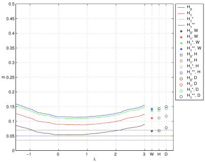
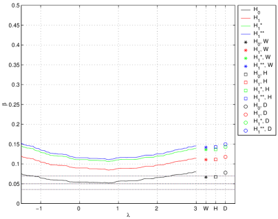
The simulation experiment is performed with R = 50000 𝑅 50000 R=50000 T ( h ) ∈ { W ( h ) ( 𝜽 ~ , 𝜽 ^ ) T^{(h)}\in\{W^{(h)}(\widetilde{\boldsymbol{\theta}},\widehat{\boldsymbol{\theta}}) H ( h ) ( 𝜽 ~ , 𝜽 ^ ) superscript 𝐻 ℎ ~ 𝜽 ^ 𝜽 H^{(h)}(\widetilde{\boldsymbol{\theta}},\widehat{\boldsymbol{\theta}}) D ( h ) ( 𝜽 ¯ , 𝜽 ~ , 𝜽 ^ ) } D^{(h)}(\overline{\boldsymbol{\theta}},\widetilde{\boldsymbol{\theta}},\widehat{\boldsymbol{\theta}})\} h = 1 , … , R ℎ 1 … 𝑅
h=1,...,R T ( h ) ∈ { T λ ( h ) ( 𝒑 ¯ , 𝒑 ( 𝜽 ~ ) , 𝒑 ( 𝜽 ^ ) ) , S λ ( h ) ( 𝒑 ( 𝜽 ~ ) , 𝒑 ( 𝜽 ^ ) ) } λ ∈ I superscript 𝑇 ℎ subscript superscript subscript 𝑇 𝜆 ℎ ¯ 𝒑 𝒑 ~ 𝜽 𝒑 ^ 𝜽 superscript subscript 𝑆 𝜆 ℎ 𝒑 ~ 𝜽 𝒑 ^ 𝜽 𝜆 𝐼 T^{(h)}\in\{T_{\lambda}^{(h)}(\overline{\boldsymbol{p}},\boldsymbol{p}(\widetilde{\boldsymbol{\theta}}),\boldsymbol{p}(\widehat{\boldsymbol{\theta}})),S_{\lambda}^{(h)}(\boldsymbol{p}(\widetilde{\boldsymbol{\theta}}),\boldsymbol{p}(\widehat{\boldsymbol{\theta}}))\}_{\lambda\in I} h = 1 , … , R ℎ 1 … 𝑅
h=1,...,R I = ( − 1.5 , 3 ) 𝐼 1.5 3 I=(-1.5,3) α = 0.05 𝛼 0.05 \alpha=0.05
∑ h = 1 R I { p - v a l u e ( T ( h ) ) ≤ α } R , superscript subscript ℎ 1 𝑅 𝐼 𝑝 - 𝑣 𝑎 𝑙 𝑢 𝑒 superscript 𝑇 ℎ 𝛼 𝑅 \frac{\sum_{h=1}^{R}I\{p\text{-}value(T^{(h)})\leq\alpha\}}{R}, (31)
where I { ∙ } 𝐼 ∙ I\{\bullet\} α ^ T subscript ^ 𝛼 𝑇 \widehat{\alpha}_{T} T ∈ { W ( 𝜽 ~ , 𝜽 ^ ) , H ( 𝜽 ~ , 𝜽 ^ ) , D ( 𝜽 ¯ , 𝜽 ~ , 𝜽 ^ ) , T λ ( 𝒑 ¯ , 𝒑 ( 𝜽 ~ ) , 𝒑 ( 𝜽 ^ ) ) , S λ ( 𝒑 ( 𝜽 ~ ) , 𝒑 ( 𝜽 ^ ) ) } λ ∈ I 𝑇 subscript 𝑊 ~ 𝜽 ^ 𝜽 𝐻 ~ 𝜽 ^ 𝜽 𝐷 ¯ 𝜽 ~ 𝜽 ^ 𝜽 subscript 𝑇 𝜆 ¯ 𝒑 𝒑 ~ 𝜽 𝒑 ^ 𝜽 subscript 𝑆 𝜆 𝒑 ~ 𝜽 𝒑 ^ 𝜽 𝜆 𝐼 T\in\{W(\widetilde{\boldsymbol{\theta}},\widehat{\boldsymbol{\theta}}),H(\widetilde{\boldsymbol{\theta}},\widehat{\boldsymbol{\theta}}),D(\overline{\boldsymbol{\theta}},\widetilde{\boldsymbol{\theta}},\widehat{\boldsymbol{\theta}}),T_{\lambda}(\overline{\boldsymbol{p}},\boldsymbol{p}(\widetilde{\boldsymbol{\theta}}),\boldsymbol{p}(\widehat{\boldsymbol{\theta}})),S_{\lambda}(\boldsymbol{p}(\widetilde{\boldsymbol{\theta}}),\boldsymbol{p}(\widehat{\boldsymbol{\theta}}))\}_{\lambda\in I} β ^ T subscript ^ 𝛽 𝑇 \widehat{\beta}_{T} α ^ T subscript ^ 𝛼 𝑇 \widehat{\alpha}_{T} β ^ T subscript ^ 𝛽 𝑇 \widehat{\beta}_{T} 31
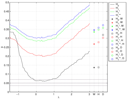
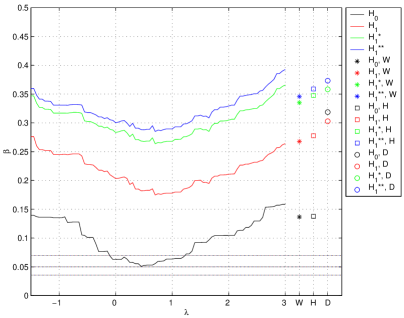
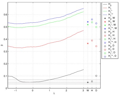
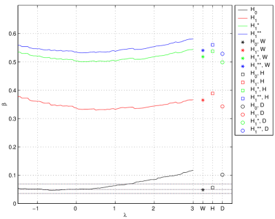
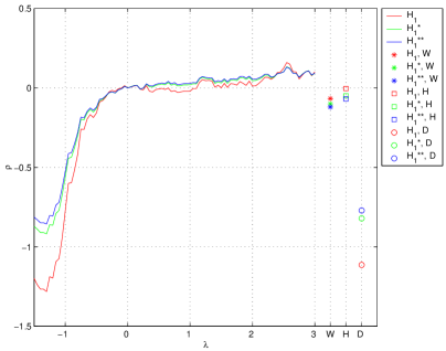
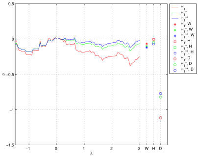
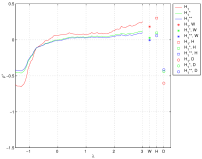
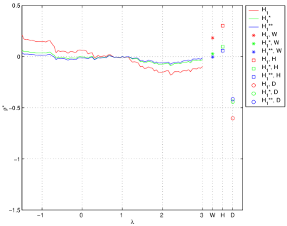
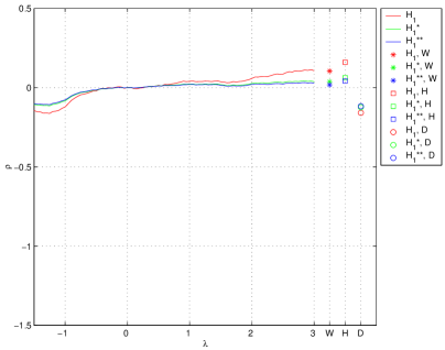
In Figures 1 2 α ^ T subscript ^ 𝛼 𝑇 \widehat{\alpha}_{T} β ^ T subscript ^ 𝛽 𝑇 \widehat{\beta}_{T} T λ ( 𝒑 ¯ , 𝒑 ( 𝜽 ~ ) , 𝒑 ( 𝜽 ^ ) ) subscript 𝑇 𝜆 ¯ 𝒑 𝒑 ~ 𝜽 𝒑 ^ 𝜽 T_{\lambda}(\overline{\boldsymbol{p}},\boldsymbol{p}(\widetilde{\boldsymbol{\theta}}),\boldsymbol{p}(\widehat{\boldsymbol{\theta}})) S λ ( 𝒑 ( 𝜽 ~ ) , 𝒑 ( 𝜽 ^ ) ) subscript 𝑆 𝜆 𝒑 ~ 𝜽 𝒑 ^ 𝜽 S_{\lambda}(\boldsymbol{p}(\widetilde{\boldsymbol{\theta}}),\boldsymbol{p}(\widehat{\boldsymbol{\theta}})) W ( 𝜽 ~ , 𝜽 ^ ) 𝑊 ~ 𝜽 ^ 𝜽 W(\widetilde{\boldsymbol{\theta}},\widehat{\boldsymbol{\theta}}) H ( 𝜽 ~ , 𝜽 ^ ) 𝐻 ~ 𝜽 ^ 𝜽 H(\widetilde{\boldsymbol{\theta}},\widehat{\boldsymbol{\theta}}) D ( 𝜽 ¯ , 𝜽 ~ , 𝜽 ^ ) 𝐷 ¯ 𝜽 ~ 𝜽 ^ 𝜽 D(\overline{\boldsymbol{\theta}},\widetilde{\boldsymbol{\theta}},\widehat{\boldsymbol{\theta}}) T λ ( 𝒑 ¯ , 𝒑 ( 𝜽 ~ ) , 𝒑 ( 𝜽 ^ ) ) subscript 𝑇 𝜆 ¯ 𝒑 𝒑 ~ 𝜽 𝒑 ^ 𝜽 T_{\lambda}(\overline{\boldsymbol{p}},\boldsymbol{p}(\widetilde{\boldsymbol{\theta}}),\boldsymbol{p}(\widehat{\boldsymbol{\theta}})) S λ ( 𝒑 ( 𝜽 ~ ) , 𝒑 ( 𝜽 ^ ) ) subscript 𝑆 𝜆 𝒑 ~ 𝜽 𝒑 ^ 𝜽 S_{\lambda}(\boldsymbol{p}(\widetilde{\boldsymbol{\theta}}),\boldsymbol{p}(\widehat{\boldsymbol{\theta}})) α ^ T subscript ^ 𝛼 𝑇 \widehat{\alpha}_{T}
| logit ( 1 − α ^ T ) − logit ( 1 − α ) | ≤ ϵ logit 1 subscript ^ 𝛼 𝑇 logit 1 𝛼 italic-ϵ \left|\mathrm{logit}(1-\widehat{\alpha}_{T})-\mathrm{logit}(1-\alpha)\right|\leq\epsilon
for ϵ ∈ { 0.35 , 0.7 } italic-ϵ 0.35 0.7 \epsilon\in\{0.35,0.7\} ϵ = 0.35 italic-ϵ 0.35 \epsilon=0.35 ϵ = 0.7 italic-ϵ 0.7 \epsilon=0.7 ϵ = 0.35 italic-ϵ 0.35 \epsilon=0.35 α = 0.05 𝛼 0.05 \alpha=0.05 β ^ T 0 − α ^ T 0 subscript ^ 𝛽 subscript 𝑇 0 subscript ^ 𝛼 subscript 𝑇 0 \widehat{\beta}_{T_{0}}-\widehat{\alpha}_{T_{0}} β ^ S 1 − α ^ S 1 subscript ^ 𝛽 subscript 𝑆 1 subscript ^ 𝛼 subscript 𝑆 1 \widehat{\beta}_{S_{1}}-\widehat{\alpha}_{S_{1}} T 0 ( 𝒑 ¯ , 𝒑 ( 𝜽 ~ ) , 𝒑 ( 𝜽 ^ ) ) = G 2 subscript 𝑇 0 ¯ 𝒑 𝒑 ~ 𝜽 𝒑 ^ 𝜽 superscript 𝐺 2 T_{0}(\overline{\boldsymbol{p}},\boldsymbol{p}(\widetilde{\boldsymbol{\theta}}),\boldsymbol{p}(\widehat{\boldsymbol{\theta}}))=G^{2}
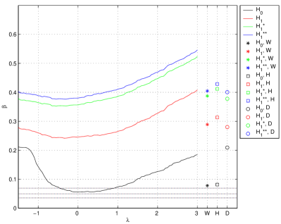
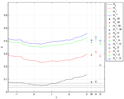
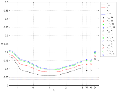
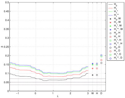
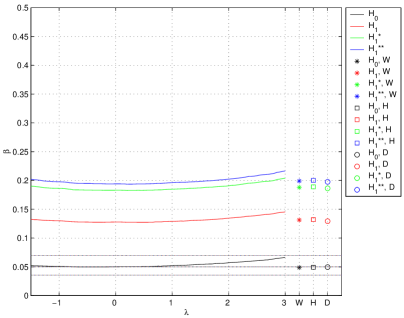
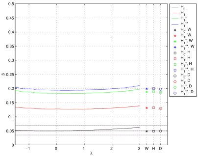
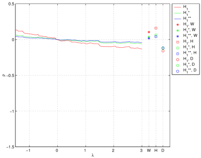
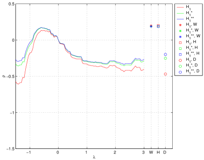
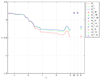
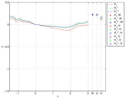
ρ T = ( β ^ T − α ^ T ) − ( β ^ T 0 − α ^ T 0 ) β ^ T 0 − α ^ T 0 subscript 𝜌 𝑇 subscript ^ 𝛽 𝑇 subscript ^ 𝛼 𝑇 subscript ^ 𝛽 subscript 𝑇 0 subscript ^ 𝛼 subscript 𝑇 0 subscript ^ 𝛽 subscript 𝑇 0 subscript ^ 𝛼 subscript 𝑇 0 \rho_{T}=\frac{\left(\widehat{\beta}_{T}-\widehat{\alpha}_{T}\right)-\left(\widehat{\beta}_{T_{0}}-\widehat{\alpha}_{T_{0}}\right)}{\widehat{\beta}_{T_{0}}-\widehat{\alpha}_{T_{0}}} (32)
or the Bartholomew’s test (S 1 ( 𝒑 ( 𝜽 ~ ) , 𝒑 ( 𝜽 ^ ) ) = X 2 subscript 𝑆 1 𝒑 ~ 𝜽 𝒑 ^ 𝜽 superscript 𝑋 2 S_{1}(\boldsymbol{p}(\widetilde{\boldsymbol{\theta}}),\boldsymbol{p}(\widehat{\boldsymbol{\theta}}))=X^{2}
ρ T ∗ = ( β ^ T − α ^ T ) − ( β ^ S 1 − α ^ S 1 ) β ^ S 1 − α ^ S 1 superscript subscript 𝜌 𝑇 ∗ subscript ^ 𝛽 𝑇 subscript ^ 𝛼 𝑇 subscript ^ 𝛽 subscript 𝑆 1 subscript ^ 𝛼 subscript 𝑆 1 subscript ^ 𝛽 subscript 𝑆 1 subscript ^ 𝛼 subscript 𝑆 1 \rho_{T}^{\ast}=\frac{\left(\widehat{\beta}_{T}-\widehat{\alpha}_{T}\right)-\left(\widehat{\beta}_{S_{1}}-\widehat{\alpha}_{S_{1}}\right)}{\widehat{\beta}_{S_{1}}-\widehat{\alpha}_{S_{1}}} (33)
are considered. In Table 3 S 1 = X 2 subscript 𝑆 1 superscript 𝑋 2 S_{1}=X^{2} T 0 = G 2 subscript 𝑇 0 superscript 𝐺 2 T_{0}=G^{2} ρ S 1 < 0 subscript 𝜌 subscript 𝑆 1 0 \rho_{S_{1}}<0 T 0 = G 2 subscript 𝑇 0 superscript 𝐺 2 T_{0}=G^{2} S 1 = X 2 subscript 𝑆 1 superscript 𝑋 2 S_{1}=X^{2} 3 4 32 ρ S 1 > 0 subscript 𝜌 subscript 𝑆 1 0 \rho_{S_{1}}>0 T 0 = G 2 subscript 𝑇 0 superscript 𝐺 2 T_{0}=G^{2} S 1 = X 2 subscript 𝑆 1 superscript 𝑋 2 S_{1}=X^{2} 3 4 33
Table 3: Efficiency of the Bartholomew’s test with respect to the likelihood ratio test.
{ T λ ( 𝒑 ¯ , 𝒑 ( 𝜽 ~ ) , 𝒑 ( 𝜽 ^ ) ) } λ ∈ ( − 1.5 , 3 ) subscript subscript 𝑇 𝜆 ¯ 𝒑 𝒑 ~ 𝜽 𝒑 ^ 𝜽 𝜆 1.5 3 \{T_{\lambda}(\overline{\boldsymbol{p}},\boldsymbol{p}(\widetilde{\boldsymbol{\theta}}),\boldsymbol{p}(\widehat{\boldsymbol{\theta}}))\}_{\lambda\in(-1.5,3)} { S λ ( 𝒑 ( 𝜽 ~ ) , 𝒑 ( 𝜽 ^ ) ) } λ ∈ ( − 1.5 , 3 ) subscript subscript 𝑆 𝜆 𝒑 ~ 𝜽 𝒑 ^ 𝜽 𝜆 1.5 3 \{S_{\lambda}(\boldsymbol{p}(\widetilde{\boldsymbol{\theta}}),\boldsymbol{p}(\widehat{\boldsymbol{\theta}}))\}_{\lambda\in(-1.5,3)}
W ( 𝜽 ~ , 𝜽 ^ ) 𝑊 ~ 𝜽 ^ 𝜽 W(\widetilde{\boldsymbol{\theta}},\widehat{\boldsymbol{\theta}}) H ( 𝜽 ~ , 𝜽 ^ ) 𝐻 ~ 𝜽 ^ 𝜽 H(\widetilde{\boldsymbol{\theta}},\widehat{\boldsymbol{\theta}}) D ( 𝜽 ¯ , 𝜽 ~ , 𝜽 ^ ) 𝐷 ¯ 𝜽 ~ 𝜽 ^ 𝜽 D(\overline{\boldsymbol{\theta}},\widetilde{\boldsymbol{\theta}},\widehat{\boldsymbol{\theta}})
sc A-0 (black), sc A-1 (red), sc A-2 (green), sc A-3
(blue)
sc B-0 (black), sc B-1 (red), sc B-2 (green), sc B-3
(blue)
sc C-0 (black), sc C-1 (red), sc C-2 (green), sc C-3
(blue)
Figure 1: Simulated sizes (black) and powers (red, green, blue) for scenarios A,B,C (small/big proportions).
{ T λ ( 𝒑 ¯ , 𝒑 ( 𝜽 ~ ) , 𝒑 ( 𝜽 ^ ) ) } λ ∈ ( − 1.5 , 3 ) subscript subscript 𝑇 𝜆 ¯ 𝒑 𝒑 ~ 𝜽 𝒑 ^ 𝜽 𝜆 1.5 3 \{T_{\lambda}(\overline{\boldsymbol{p}},\boldsymbol{p}(\widetilde{\boldsymbol{\theta}}),\boldsymbol{p}(\widehat{\boldsymbol{\theta}}))\}_{\lambda\in(-1.5,3)} { S λ ( 𝒑 ( 𝜽 ~ ) , 𝒑 ( 𝜽 ^ ) ) } λ ∈ ( − 1.5 , 3 ) subscript subscript 𝑆 𝜆 𝒑 ~ 𝜽 𝒑 ^ 𝜽 𝜆 1.5 3 \{S_{\lambda}(\boldsymbol{p}(\widetilde{\boldsymbol{\theta}}),\boldsymbol{p}(\widehat{\boldsymbol{\theta}}))\}_{\lambda\in(-1.5,3)}
W ( 𝜽 ~ , 𝜽 ^ ) 𝑊 ~ 𝜽 ^ 𝜽 W(\widetilde{\boldsymbol{\theta}},\widehat{\boldsymbol{\theta}}) H ( 𝜽 ~ , 𝜽 ^ ) 𝐻 ~ 𝜽 ^ 𝜽 H(\widetilde{\boldsymbol{\theta}},\widehat{\boldsymbol{\theta}}) D ( 𝜽 ¯ , 𝜽 ~ , 𝜽 ^ ) 𝐷 ¯ 𝜽 ~ 𝜽 ^ 𝜽 D(\overline{\boldsymbol{\theta}},\widetilde{\boldsymbol{\theta}},\widehat{\boldsymbol{\theta}})
sc D-0 (black), sc D-1 (red), sc D-2 (green), sc D-3
(blue)
sc E-0 (black), sc E-1 (red), sc E-2 (green), sc E-3
(blue)
sc F-0 (black), sc F-1 (red), sc F-2 (green), sc F-3
(blue)
Figure 2: Simulated sizes (black) and powers (red, green, blue) for scenarios D,E,F (intermediate proportions).
{ T λ ( 𝒑 ¯ , 𝒑 ( 𝜽 ~ ) , 𝒑 ( 𝜽 ^ ) ) } λ ∈ ( − 1.5 , 3 ) subscript subscript 𝑇 𝜆 ¯ 𝒑 𝒑 ~ 𝜽 𝒑 ^ 𝜽 𝜆 1.5 3 \{T_{\lambda}(\overline{\boldsymbol{p}},\boldsymbol{p}(\widetilde{\boldsymbol{\theta}}),\boldsymbol{p}(\widehat{\boldsymbol{\theta}}))\}_{\lambda\in(-1.5,3)} { S λ ( 𝒑 ( 𝜽 ~ ) , 𝒑 ( 𝜽 ^ ) ) } λ ∈ ( − 1.5 , 3 ) subscript subscript 𝑆 𝜆 𝒑 ~ 𝜽 𝒑 ^ 𝜽 𝜆 1.5 3 \{S_{\lambda}(\boldsymbol{p}(\widetilde{\boldsymbol{\theta}}),\boldsymbol{p}(\widehat{\boldsymbol{\theta}}))\}_{\lambda\in(-1.5,3)}
W ( 𝜽 ~ , 𝜽 ^ ) 𝑊 ~ 𝜽 ^ 𝜽 W(\widetilde{\boldsymbol{\theta}},\widehat{\boldsymbol{\theta}}) H ( 𝜽 ~ , 𝜽 ^ ) 𝐻 ~ 𝜽 ^ 𝜽 H(\widetilde{\boldsymbol{\theta}},\widehat{\boldsymbol{\theta}}) D ( 𝜽 ¯ , 𝜽 ~ , 𝜽 ^ ) 𝐷 ¯ 𝜽 ~ 𝜽 ^ 𝜽 D(\overline{\boldsymbol{\theta}},\widetilde{\boldsymbol{\theta}},\widehat{\boldsymbol{\theta}})
sc A-0 (black), sc A-1 (red), sc A-2 (green), sc A-3
(blue)
sc B-0 (black), sc B-1 (red), sc B-2 (green), sc B-3
(blue)
sc C-0 (black), sc C-1 (red), sc C-2 (green), sc C-3
(blue)
Figure 3: Efficiencies for scenarios A,B,C (small/big proportions).
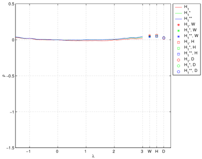
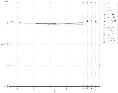
{ T λ ( 𝒑 ¯ , 𝒑 ( 𝜽 ~ ) , 𝒑 ( 𝜽 ^ ) ) } λ ∈ ( − 1.5 , 3 ) subscript subscript 𝑇 𝜆 ¯ 𝒑 𝒑 ~ 𝜽 𝒑 ^ 𝜽 𝜆 1.5 3 \{T_{\lambda}(\overline{\boldsymbol{p}},\boldsymbol{p}(\widetilde{\boldsymbol{\theta}}),\boldsymbol{p}(\widehat{\boldsymbol{\theta}}))\}_{\lambda\in(-1.5,3)} { S λ ( 𝒑 ( 𝜽 ~ ) , 𝒑 ( 𝜽 ^ ) ) } λ ∈ ( − 1.5 , 3 ) subscript subscript 𝑆 𝜆 𝒑 ~ 𝜽 𝒑 ^ 𝜽 𝜆 1.5 3 \{S_{\lambda}(\boldsymbol{p}(\widetilde{\boldsymbol{\theta}}),\boldsymbol{p}(\widehat{\boldsymbol{\theta}}))\}_{\lambda\in(-1.5,3)}
W ( 𝜽 ~ , 𝜽 ^ ) 𝑊 ~ 𝜽 ^ 𝜽 W(\widetilde{\boldsymbol{\theta}},\widehat{\boldsymbol{\theta}}) H ( 𝜽 ~ , 𝜽 ^ ) 𝐻 ~ 𝜽 ^ 𝜽 H(\widetilde{\boldsymbol{\theta}},\widehat{\boldsymbol{\theta}}) D ( 𝜽 ¯ , 𝜽 ~ , 𝜽 ^ ) 𝐷 ¯ 𝜽 ~ 𝜽 ^ 𝜽 D(\overline{\boldsymbol{\theta}},\widetilde{\boldsymbol{\theta}},\widehat{\boldsymbol{\theta}})
sc C-0 (black), sc C-1 (red), sc C-2 (green), sc C-3
(blue)
sc D-0 (black), sc D-1 (red), sc D-2 (green), sc D-3
(blue)
sc E-0 (black), sc E-1 (red), sc E-2 (green), sc E-3
(blue)
Figure 4: Efficiencies for scenarios C,D,E (intermediate proportions).
In view of the plots, it is possible to propose test-statistics with better
performance in comparison with G 2 superscript 𝐺 2 G^{2} X 2 superscript 𝑋 2 X^{2} 1 3 T 2 3 ( 𝒑 ¯ , 𝒑 ( 𝜽 ~ ) , 𝒑 ( 𝜽 ^ ) ) subscript 𝑇 2 3 ¯ 𝒑 𝒑 ~ 𝜽 𝒑 ^ 𝜽 T_{\frac{2}{3}}(\overline{\boldsymbol{p}},\boldsymbol{p}(\widetilde{\boldsymbol{\theta}}),\boldsymbol{p}(\widehat{\boldsymbol{\theta}})) W ( 𝜽 ~ , 𝜽 ^ ) 𝑊 ~ 𝜽 ^ 𝜽 W(\widetilde{\boldsymbol{\theta}},\widehat{\boldsymbol{\theta}}) H ( 𝜽 ~ , 𝜽 ^ ) 𝐻 ~ 𝜽 ^ 𝜽 H(\widetilde{\boldsymbol{\theta}},\widehat{\boldsymbol{\theta}}) T − 0.5 ( 𝒑 ¯ , 𝒑 ( 𝜽 ~ ) , 𝒑 ( 𝜽 ^ ) ) subscript 𝑇 0.5 ¯ 𝒑 𝒑 ~ 𝜽 𝒑 ^ 𝜽 T_{-0.5}(\overline{\boldsymbol{p}},\boldsymbol{p}(\widetilde{\boldsymbol{\theta}}),\boldsymbol{p}(\widehat{\boldsymbol{\theta}}))