Correlation between magnetic interactions and domain structure in A1 FePt ferromagnetic thin films

Abstract

We have investigated the relationship between the domain structure and the magnetic interactions in a series of FePt ferromagnetic thin films of varying thickness. As-made films grow in the magnetically soft and chemically disordered A1 phase that may have two distinct domain structures. Above a critical thickness $d_{cr}\sim 30$ nm the presence of an out of plane anisotropy induces the formation of stripes, while for $d<d_{cr}$ planar domains occur.

Magnetic interactions have been characterized using the well known DCD-IRM remanence protocols, $\delta M$ plots, and magnetic viscosity measurements. We have observed a strong correlation between the domain configuration and the sign of the magnetic interactions. Planar domains are associated with positive exchange-like interactions, while stripe domains have a strong negative dipolar-like contribution. In this last case we have found a close correlation between the interaction parameter and the surface dipolar energy of the stripe domain structure. Using time dependent magnetic viscosity measurements, we have also estimated an average activation volume for magnetic reversal, $\langle V_{ac}\rangle\sim 1.37\times 10^{4}$ nm${}^{3},$ which is approximately independent of the film thickness or the stripe period.

I Introduction

Ferromagnetic thin films exhibiting a magnetic domain structure in the form of thin parallel stripes have been the subject of intense research in the last few decades, both experimentallySaito ; Hehn ; Gehanno2 ; Okamoto ; ButeraMFM ; FeGa and theoretically.Kooy ; Murayama ; Sukstanskii ; Brucas ; Hubert This kind of structure is observed in films that present an out of plane anisotropy component (due to stress, crystalline texture, interfacial or other effects) and in a simplified picture it can be described as a periodic pattern of parallel in-plane magnetized regions in which the magnetization has a relatively small component that points alternatively in the two directions that are normal to the film plane. A stripe (or bubble) pattern is generally observed for all film thicknesses when the perpendicular anisotropy energy constant, $K_{\perp},$ is larger than the demagnetizing shape energy, $2\pi M_{s}^{2}$, ($M_{s}$ is the saturation magnetization) but can also be found below a critical thickness $d_{cr}$ when $Q=K_{\perp}/2\pi M_{s}^{2}$ is smaller than one. The transition from planar to stripe domains at $d=$ $d_{cr},$ is due to the minimization of the total magnetic energy which can include the contribution of anisotropy, demagnetizing, domain wall and Zeeman (for $H\neq 0$) terms. The critical thickness depends on the material properties such as the effective anisotropy, the saturation magnetization and the exchange stiffness constant, and also on the external field. There are several models for the calculation of $d_{cr},$ see for example Refs. [Sukstanskii, ; Brucas, ; Hubert, ], that predict larger values of $d_{cr}$ in materials with a large saturation magnetization, a large exchange, or a small anisotropy. The value of the critical thickness is in the range of 20-30 nm for Co,Hehn partially ordered FePdGehanno2 or disordered FePt filmsButeraMFM ; Butera1 ; Butera2 ; ButeraFMR ; ButeraSSW ; Jonas ; ButeraFMR2 , and can take larger values (of the order of 200 nm) in films with lower anisotropy such as permalloy.Ramos Films with stripe domains have characteristic $M$ vs. $H$ in-plane loops in which the following features are often observed:Murayama ; ButeraMFM $i)$ the low field part of the curve increases almost linearly from remanence until the saturation field is reached. This in-plane saturation field was shown to increase with film thickness following approximately the relationship $H_{\mathrm{sat}\parallel}=H_{\mathrm{sat}\perp}\left[1-d_{cr}/\left(d\sqrt{1+Q}\right)\right],$ with $H_{\mathrm{sat}\perp}=2K_{\perp}/M_{s}.$ $ii)$ Due to the formation of the stripe structure the in-plane coercivity increases abruptly and the remanence decreases considerably above $d_{cr}.$ $iii)$ For $d\geq d_{cr}$ rotatable anisotropy, i.e. the alignment of the stripe structure at remanence in the direction of a previously applied field, is observed. The magnitude of this anisotropy also increases with film thickness and is usually characterized by a field $H_{\mathrm{rot}}$. $iv)$ The period of the stripe structure increases approximately as the square root of the film thickness, $\lambda_{s}\varpropto\sqrt{d}.$

The study of the magnetic interactions present in films in which a crossover from a planar to a striped magnetic domain structure is observed can then give a deeper insight to understand this behavior. Both Henkel plotsSpratt and delta$-M$ ($\delta M)$ curves,Kelly ; Otero together with the magnetic viscosity, $S,$Wohlfarth ; Wohlfarth2 can be used to estimate the sign of the magnetic interactions and the magnetic reversal volumes in the samples. Magnetic interactions have been widely studied in small particles,Che thin continuous films,Che granular systemsCoAg and nanostructured filmsNCA using magnetic remanence measurements.

The $\delta M$ curve is defined as the difference between two remanence curves:

$$\delta M=2M_{r}-1-M_{d},$$ (1)

where the $M_{r}$ curve (also known as the isothermal remanent magnetization, IRM) is obtained by starting from a state of zero remanence, erased following a well defined protocol, and then measuring the magnetization at zero field after applying fields of increasing magnitude. The $M_{d}$ (or dc demagnetization, DCD) curve is obtained by saturating the sample in a negative field and then repeating the same procedure as for the $M_{r}$ curves. These two curves are usually normalized to the remanence saturation value ($M_{R}$) and labeled as $m_{r}$ and $m_{d}$. In the case of a noninteracting system Wohlfarth predictedWohlfarth2 that the two remanence curves should be identical and hence $\delta M=0$. If $\delta M\neq 0$ the effects of magnetic interactions can been accounted for using a phenomenological modelChe for the effective interaction field, $h_{int},$ that takes into consideration dipolar-like (demagnetizing) and exchange-like (magnetizing) interactions. In this model $h_{int}=\alpha m+\beta(1-m^{2}),$ which means that the interaction field has a linear dependence with $m$ (which can be both $m_{r}$ or $m_{d}$) with a slope of magnitude $\alpha$. This parameter can be either positive or negative depending on the dominant type of interaction, exchange-like or dipolar-like, respectively. The term with the parameter $\beta$ accounts for first order interaction field fluctuations from the mean field. A numerical method to calculate $\alpha$ and $\beta$ is described in Ref. [Che, ], but they can be more easily obtained from the experimental data following the procedure of Ref. [Harrell, ]

$$\alpha=\int_{0}^{\infty}\delta M\,dh,\qquad\beta=\alpha/(3m_{r}^{0}-1).$$ (2)

In the above expression $h$ is the applied field normalized to the remanent coercivity $H_{C}^{\mathrm{rem}}$ (defined as the reverse negative field that, after saturation in the positive direction, produces a zero magnetization at zero field) and $m_{r}^{0}$ is the remanent magnetization at the point where $\delta M$ curves cross zero.

In order to get a deeper insight in the magnetic behavior, remanence measurements are often complemented with magnetic relaxation experiments. When a sample is magnetized in a negative saturating field and after that a positive field is applied, the magnitude of $M$ often varies linearly with the logarithm of time $t$. Changes in $M$ are due to thermally assisted processes that provide the necessary energy to overcome the barrier energy of magnitude $E$. The proportionality parameter is the magnetic viscosity $S$ and the relationship is often written as:Street

$$M(t,H)=M(t_{0},H)+S(H)\ln(t/t_{0}),$$ (3)

with $t_{0}$ the initial time and $M(t_{0},H)$ the initial value of $M$ at $t=t_{0}$ for a given $H.$ The viscosity $S$ can be shown to depend on temperature, $T$, saturation magnetization, $M_{s}$, and the distribution of activation energies, $f(E)$, in the following wayGaunt1

$$S=2M_{s}k_{B}Tf(E).$$ (4)

The magnetic viscosity depends also on the forward applied field, through the dependence of $f(E)$ on $H,$ and is generally maximum for an applied field $H_{S}$ which is close to the macroscopic coercive field $H_{C}$. Viscosity and remanence measurements can be related using the field derivative of the DCD curve, known as the irreversible susceptibilityGaunt2

$$\chi_{irr}=\frac{\partial M_{d}}{\partial H}=-2M_{s}f(E)\left(\frac{dE}{dH}\right).$$ (5)

The variation of the activation energy with the magnetic field can be related to the so called activation volume, $\left|\frac{dE}{dH}\right|=cV_{ac}M_{s}$, where $c$ is a constant of the order of unity and its value depends on the kind of system that is under consideration. Simple calculationsGaunt2 for monodomain particles or strong domain-wall pinning give $c=1,$ while for weak domain-wall pinning $c=2.$ If demagnetizing effects are considered,Ng $c=4$ for strong pinning and $c\geq 2$ for weak pinning. Using Eqs. [4] and [5] the activation volume can be written as:

$$V_{ac}=\frac{k_{B}T\chi_{irr}}{cM_{s}S}.$$ (6)

In the case of thin films in which the magnetization changes by a process of domain wall motion, the activation volume can be interpreted as the volume swept by a single jump between pinning centers. This volume is usually related with the fluctuation field, $H_{f}$, defined as:Ng

$$H_{f}=\frac{S}{\chi_{irr}}=-\frac{k_{B}T}{dE/dH}=\frac{k_{B}T}{cM_{s}}\frac{1}{V_{ac}}.$$ (7)

Magnetic interactions in FePt have been investigated in different systems, including continuous films,Li ; Jeong annealed multilayers,Luo exchange-coupled bilayers,Pernechele granular films,Wei ; Wei2 and nanoparticles,Gao all in the atomically ordered L1₀ phase. Negative interparticle interactions were reported in the cases of films, annealed multilayers and nanoparticles, when the external field was applied parallel to the in-plane direction (these films show in-plane anisotropy). On the other hand, continuous films exhibiting out of plane anisotropyJeong ; Wei present positive $\delta M$ curves when remanence curves are measured perpendicular to the film plane. Magnetic relaxation has been reported in the case of exchange-coupled Fe/FePt bilayers,Pernechele annealed Fe/Pt multilayers,Luo and polycrystalline thin filmsJeong all of them in the hard magnetic phase. For a single layer of 10 nm of FePt with an average grain size of $\sim 20$ nm, the authors in Ref. [Pernechele, ] reported $V_{ac}\sim$ 12500 nm${}^{3}.$ In the second case the authors estimated $V_{ac}\sim$ 1200 nm³ for a multilayer with a total thickness of 15 nm. In the last case an activation volume $V_{ac}\sim$ 400 nm³ was estimated for a film 5 nm thick with a crystalline grain size of 10 nm. This last sample presented a maze structure of magnetic domains at remanence, consisting of irregular elongated regions magnetized perpendicular to the film plane with a length of several micrometers and a width of 100-150 nm. Assuming spherical reversal volumes, the corresponding ”activation diameters” are $d_{ac}=29$, 13, and 9 nm, respectively. Note that if the activation volume is divided by the film thickness, and cylindrical domains are assumed, the resulting ”activation length” is in the range of 40 nm for the first sample and 9 nm in the last two systems.

As far as we know, magnetic interactions and time dependent effects in FePt films in the A1 disordered phase have not been yet characterized. The possibility to tune the domain structure by varying the film thickness can be used to study how these effects are affected by the way in which the magnetic domains order. In the following sections we present a detailed experimental study in a series of as-made FePt thin films of different thicknesses in which the magnetic interactions have been investigated by means of DCD-IRM, delta-$M$ plots and magnetic viscosity measurements.

II Experimental details

FePt films have been fabricated by dc magnetron sputtering on naturally oxidized Si (100) substrates. A detailed description of the preparation and the structural characterization can be found in Ref. [ButeraMFM, ]. The samples were deposited from an FePt alloy target with a nominal atomic composition of 50/50. We sputtered eight films with thicknesses of 9, 19, 28, 35, 42, 49, 56 and 94 nm. The samples were studied using X-Ray diffraction, transmission electron microscopy (TEM) and energy-dispersive X-Ray spectroscopy (EDS) techniques. The X-ray diffractograms showed that the samples grow in the fcc A1 crystalline phase, without traces of the ordered L1₀ structure. A [111] texture normal to the film plane was observed and comparison with stress released films revealed that as-made samples were also subjected to an in-plane compressive stress. An average crystallite grain diameter of 4 nm was obtained from TEM micrographs. The photoemission spectra indicated that the Fe/Pt atomic ratio of the films was approximately $45$/55. Stress effects are the main contribution to an effective magnetic anisotropy perpendicular to the film plane of magnitude $K_{\perp}=1.5(4)\times\ 10^{6}$ erg/cm³, which gives rise to a magnetic domain structure in the form of stripes for $d>d_{cr}\sim 30$ nm. As we have already shown in Ref. [ButeraMFM, ] using magnetic force microscopy (MFM) techniques, the half period of the stripe pattern scales with the square root of the film thickness starting at $\lambda/2\sim 45$ nm for $d=35$ nm and reaching $\lambda/2\sim 75$ nm for $d=94$ nm. For $d<d_{cr}$ an in-plane planar domain structure is observed. In both domain regimes a strong correlation between the domain configuration and the shape of the hysteresis loops was found.

The DC demagnetization (DCD), Isothermal Remanent Magnetization (IRM) and viscosity data were measured using a LakeShore model 7300 VSM, capable of a maximum field of 10000 Oe. For the DCD measurements we used the following sequence of applied fields $(-H_{sat},\Delta H,0);(-H_{sat},2\Delta H,0);...(-H_{sat},n\Delta H,0);...$ In this case a negative saturation field $-H_{sat}$ is applied before each data point is acquired at $H=0$ after applying a field $H=n\Delta H.$ In most cases we set $H_{sat}=5000$ Oe and $\Delta H\leq 10$ Oe, depending on the coercivity of the sample. A waiting time of 5 seconds was used before measuring the remanent magnetization. There is an alternative field sequence for performing DCD experiementsWang $-H_{sat};(\Delta H,0);(2\Delta H,0);...$ in which the saturation field is applied only at the beginning of the experiment. In principle, this method should be less sensitive to the waiting time and the field step $\Delta H$, and differences between the DCD and IRM curves due to viscosity effects are minimized. In our case we did not observe significant differences between both DCD sequences and decided to use the first method.

The IRM curve is obtained by starting from a demagnetized state and measuring the magnetization at zero field following the sequence $(\Delta H,0);(2\Delta H,0);...$The ideal demagnetized remanent state is the one obtained by heating the sample above the Curie temperature, $T_{C}$, and then cooling in zero field. Because of the appearance of irreversible effects in the magnetic response,Jonas our films can not be heated to $T_{C}$ $\sim 500$ K, so we adopted two different protocols to demagnetize the samples. The ”linear” demagnetization routine is the usual procedure in which the sample is saturated in one direction and a sequence of decreasing fields is applied in both senses, until zero field is reached. Films can be also demagnetized in a slowly decreasing field (from saturation to zero) while they are quickly rotated around an axis perpendicular to the magnetic field. The ”rotating” demagnetization routine usually gives a remanent state that is more disordered and isotropic in the film plane than in the linear case, resembling the state that can be obtained by cooling the sample from above $T_{C}$.

In the case of magnetic relaxation measurements films were saturated in a negative field of 5000 Oe, a positive field was then applied and kept constant during the whole experiment while the magnetization was measured in intervals of 10 seconds during approximately 30 minutes. We calculated the viscosity from the linear fit of the time variation of $M$ (Eq. 3). The same routine was repeated for several fields in the vicinity of $H_{C}$ from which the magnetic viscosity $S(H)$ is obtained.

III Experimental results and discussion

III.1 IRM and DCD measurements

In all films we have measured the IRM curves using the two demagnetizing sequences mentioned in the previous section. For films with $d\leq 19$ nm additional care must be taken in order to reach a truly demagnetized state, because the magnetization switching at $H=H_{C}$ occurs in a very narrow field range of only a few Oe. The differences between ”rotating” and ”linear” demagnetizing routines are more pronounced in thicker films. In Fig. 1 (a) we show the upper right quadrant of the hysteresis loop for the film with $d=94$ nm, together with the virgin curve obtained after demagnetizing the film using the rotating routine. It can be observed that there is a field region in which the virgin curve is not within the hysteresis loop. This effect is almost absent when the sample is demagnetized using the linear sequence and to explain it one must consider that the remanent state obtained when the sample is demagnetized using the rotating routine consists of an array of randomly oriented stripes.ButeraMFM On the other hand, in the case of the linear protocol almost all stripes are already aligned at remanence in the direction of the demagnetizing field. When the sample is saturated, rotational anisotropy imposes an easy magnetization axis along the field direction and the stripes are always aligned in that direction. Taking into account these effects one can understand why in the linear case the virgin curve stays inside the loop, while after the rotating cycle larger fields are needed to reach the same magnetization value because part of the field energy is used in aligning the stripes in the direction of the applied field.

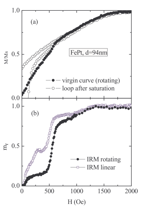
Figure 1: (color online) a) Upper right quadrant of the normalized hysteresis loop for $d=94$ nm. The virgin curve was obtained after demagnetizing the film with the ”rotating” routine. Note that there is a range of fields in which the virgin curve stays outside of the hysteresis loop. b) Normalized IRM curves obtained in the same sample after it was demagnetized using the ”linear” or the ”rotating” routines. The coercive field for this film is $H_{C}=125$ Oe.

The same differences are observed in the IRM curves, as can be seen in Fig. 1 (b). In this case starting from an initially more disordered and isotropic state (rotating routine), makes more difficult the magnetization of the sample in the direction of the applied field. Note that the magnetization process occurs in several steps. In the low field region, a relatively fast initial increase of $m_{r}$ (from $m_{r}=0$ to $m_{r}\sim 0.10)$ occurs for fields $H\lesssim H_{C}$ $\sim 125$ Oe, for $d=94$ nm. We associate these changes to domain wall movement in the small fraction of regions which were already aligned in the direction of the applied field. Then $m_{r}$ stays relatively constant until $H\sim 500$ Oe, which is more or less coincident with a kink in the virgin magnetization curve or the beginning of the reversible part of the $M-H$ loop. These features were assigned in Ref. [ButeraMFM, ] to the rotational anisotropy field $H_{\mathrm{rot}}$, the field necessary to rotate the in-plane easy axis of the stripes in the direction of the applied field. Once the stripes are aligned they can be more easily moved by the mechanism of domain wall displacement and a very large increase in $m_{r}$ (from $m_{r}=0.15$ to $m_{r}=0.75)$ occurs in the range $H=500-650$ Oe. Comparison with the hysteresis loop suggests that for $H>650$ Oe and until $H\sim 1400$ Oe irreversible changes in $m_{r}$ are probably due to the rotation of regions that are magnetized perpendicular to the film plane. The linearly demagnetized IRM curve shows similar characteristics, but the irreversible changes at low fields ($H\sim H_{C}$) are considerably larger, with $m_{r}$ reaching almost 50% of the saturation value. Above this field a rapid increase and then a more gradual approach to saturation is observed, with the same overall behavior already described for the rotating routine. In the rest of the films there are still differences between both demagnetizing protocols, but they tend to disappear as the films become thinner. For $d\leq 35$ nm both IRM curves are almost identical.

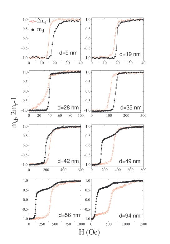
Figure 2: (color online) Normalized IRM and DCD remanence curves for the different films. In all cases the IRM data were acquired using the rotating protocol to obtain the demagnetized state.

In Fig. 2 we show the normalized DCD and IRM (starting from a rotating demagnetizing cycle) curves for all films. We have plotted $m_{d}$ and $2m_{r}-1$ in order to compare both measurements. The most significant feature that can be observed is that for $d\leq 35$ nm the IRM is above the DCD curve and the relationship is inverted for $d\geq 42$ nm. As can be deduced from Eq. 1 this implies a change in sign in the $\delta M$ curve that is indicating a change in the dominant magnetic interactions. The fact that $2m_{r}-1>$ $m_{d}$ in the case of thinner films is telling us that in these samples the saturated state can be reached more easily, i.e. the magnetic interactions favor a magnetized state. In thicker films the IRM is always below the DCD curve, which reflects that dipolar-like interactions are dominant in these samples.

From the field where $m_{d}$ and $2m_{r}-1$ curves cross zero we can extract the remanent coercivity $H_{C}^{\mathrm{rem}}$ and the IRM half reversal field, $H_{\mathrm{IRM}}$, respectively. We will show later that the normalized difference $2\left(H_{C}^{\mathrm{rem}}-H_{\mathrm{IRM}}\right)/H_{C}^{\mathrm{rem}}$ may be used as a very good estimation of the sign and magnitude of the magnetic interactions. This quantity is very similar to the so-called Interaction Field Factor, IFF$=\left(H_{C}^{\mathrm{rem}}-H_{\mathrm{IRM}}\right)/H_{C}$, differing only in the normalization variable. In Fig. 3 we plotted these two fields, together with the coercivity $H_{C}$, and the field $H_{\mathrm{rot}}$ obtained from Ref. [ButeraMFM, ]. This field is a measure of the average magnetic field needed to overcome the rotational anisotropy. For a Stoner-Wohlfarth system the two remanence fields should have the same value as $H_{C},$ which is relatively small for the thinner films, increases considerably when the stripe structure is formed, has a maximum at $d\sim 42$ nm and levels off at $H_{C}\sim 140$ Oe for larger thicknesses. This behavior is approximately followed by $H_{C}^{\mathrm{rem}},$ although as expected $H_{C}^{\mathrm{rem}}>H_{C}$, but is definitely not true for $H_{\mathrm{IRM}}$. The IRM reversal field increases continuously with film thickness giving another indication of the change in the magnetic interactions when the stripe structure is formed. As already discussed in the case of the $d=94$ nm film the IRM curve is a fingerprint of the field necessary for gradually aligning the domains that are not parallel to $H$ in the direction of the applied field. It is then expected that $H_{\mathrm{IRM}}$ values follow closely the thickness dependence of $H_{\mathrm{rot}}$, the field needed to overcome the rotational anisotropy. As can be seen in Fig. 3 both fields follow a similar trend, with the differences in the absolute values arising from the different remagnetizing mechanism that $H_{\mathrm{IRM}}$ and $H_{\mathrm{rot}}$ describe.

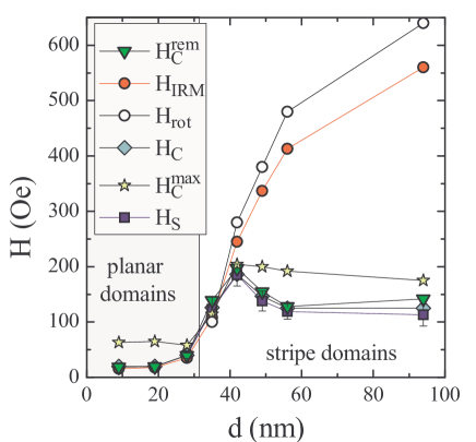
Figure 3: (color online) Room temperature remanence fields $H_{C}^{\mathrm{rem}}$ and $H_{\mathrm{IRM}}$ obtained from the zero crossing of the $m_{d}$ and $2m_{r}-1$ curves, respectively. We have also plotted for comparison the room temperature coercive field, $H_{C}$, and $H_{S},$ the field where the maximum in the magnetic viscosity is found. $H_{\mathrm{rot}}$ has been extracted from Ref. [ButeraMFM, ] and is a measure of the average field needed to rotate the stripe structure by 90^∘. $H_{C}^{\max}$ is the maximum value of $H_{C}$ in the temperature interval 4-300 K (taken from Ref. [Jonas, ]).

One of the methods to characterize qualitatively the magnetic interactions is by using the $\delta M$ plots (see Eq. 1), which reflect the deviations from the Stoner-Wohlfarth behavior. As already mentioned, if the IRM is above the DCD curve the $\delta M$ plot is positive and the interactions tend to be of the exchange type, favoring a magnetized state. Dipolar-like interactions are more important when $\delta M$ is negative. In Fig. 4 we show the $\delta M$ plots for all the studied samples as a function of the applied field (normalized by the remanent coercivity, $H_{C}^{\mathrm{rem}}$). We have used full symbols to indicate $\delta M$ plots obtained from an IRM curve that was isotropically demagnetized (rotational routine) and open symbols for the case of a linearly demagnetized sample. Note that there are differences between both $\delta M$ curves in the case of thicker films that tend to decrease gradually as the thickness is decreased. For $d\leq 35$ nm the two curves are almost coincident. These results show again explicitly that the dominant interaction changes from magnetizing to demagnetizing when the stripe structure starts to develop at $d\sim 35$ nm and they also give additional evidence of the effects of the rotational anisotropy on the IRM remanence curves. We have already shown in Figs. 2 and 3 that the fields where the DCD and IRM curves cross zero are more separated in the case of thicker films. This difference explains the shift in the minimum in the $\delta M$ plots from $H/H_{C}^{\mathrm{rem}}=1$ to at least twice this value for $d=94$ nm.

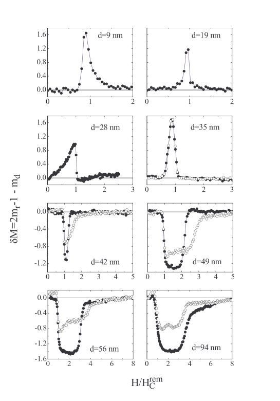
Figure 4: Delta-$M$ plots for all the studied samples that indicate the deviation from a Stoner-Wohlfarth behavior. For the thicker films we have plotted the data obtained using the two demagnetization protocols for the IRM curves with full and open symbols (rotating and linear demagnetization routines, respectively).

An estimation of the strength of the magnetic interactions can be obtained from Eq. 2, which gives the interaction parameter $\alpha$ of the Che and Bertram model.Che ; Harrell The integral of the $\delta M$ plots as a function of $d$ is presented in Fig. 5. Again we show values of $\alpha$ obtained with both demagnetizing routines. We have plotted in the same figure the quantity $\alpha_{H}=2\left(H_{C}^{\mathrm{rem}}-H_{\mathrm{IRM}}\right)/H_{C}^{\mathrm{rem}}$ which may be also used to estimate the magnetic interactions. In the case of perfectly square $m_{d}$ and $2m_{r}-1$ curves, the values of $\alpha$ and $\alpha_{H}$ should be the same because the $\delta M$ plot is rectangular with an area $2\left(H_{C}^{\mathrm{rem}}-H_{\mathrm{IRM}}\right).$ Due to the different distribution of switching fields in the IRM and DCD curves, the values of $\alpha$ differ from this simple estimation but, as can be observed in Fig. 5, the values and the shape of the curves of $\alpha$ and $\alpha_{H}$ as a function of film thickness are very similar, confirming that $\alpha_{H}$ is also a very reasonable parameter for the estimation of the magnetic interactions.

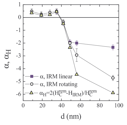
Figure 5: (color online) Interaction parameter $\alpha$ as a function of film thickness obtained from the integration of the $\delta M$ plots. Open symbols correspond to $\alpha$ values obtained from isotropically demagnetized (rotating routine) IRM curves while full symbol data were obtained from linearly demagnetized samples. The magnitude $\alpha_{H}=2(H_{C}^{\mathrm{rem}}-H_{\mathrm{IRM}})/H_{C}^{\mathrm{rem}}$ is plotted for comparison and it is found to be quite similar to $\alpha$.

A dimensional analysis of Eq. 2 reveals that the interaction parameter $\alpha$ may be associated to a normalized energy and hence could be correlated with the dominant energy contribution to the magnetic domain configuration. In the case of domains formed by parallel slabs of size $l$ magnetized perpendicular to the film plane (see the sketch in Fig. 6) it is possible to calculateChikazumi the magnetostatic energy per unit surface area as $E_{S}[\mathrm{erg}/\mathrm{cm}^{2}]=0.374M_{\perp}^{2}l.$ We can estimate this energy for the different films that show a stripe structure by identifying the thickness of the slabs with the values of the half period of the stripe structure ($l=\lambda/2),$ and estimating the component of the magnetization perpendicular to the film plane as $M_{\perp}(d)/M_{s}=M_{r\perp}(d)/M_{s}\sim\sqrt{1-[M_{r\parallel}(d)/M_{r\parallel}(d=28)]^{2}}.$ The thickness dependence of $\lambda/2$ and $M_{r\perp}$ is shown in the inset of 6. In the last formula $M_{r\parallel}(d)$ is the remanence in the direction of the applied field (obtained from the saturation value of DCD or IRM measurements) and was normalized by $M_{r\parallel}(d=28$ nm$)$ instead of $M_{s}$ to consider that there is always a small component of $M$ that is neither parallel to the anisotropy axis induced by $H$ nor parallel to the film normal. In the main panel of Fig. 6 we plotted the interaction parameter $\alpha$ as a function of $E_{S}$ for $d\geq 35$ nm and found that there is a good linear correlation between both magnitudes, indicating that for films with $d\geq d_{cr}$ it is energetically favorable to form a stripe structure which has a magnetostatic energy that increases with the stripe period (and the film thickness).

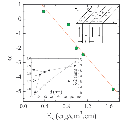
Figure 6: (color online) Dependence of the interaction parameter $\alpha$ (obtained using the rotating routine) as a function of the surface magnetostatic energy of the domain configuration sketched in the inset. We also show the dependence of the perpendicular remanence and the stripe half period, taken from Ref. [ButeraMFM, ].

III.2
Magnetic viscosity measurements

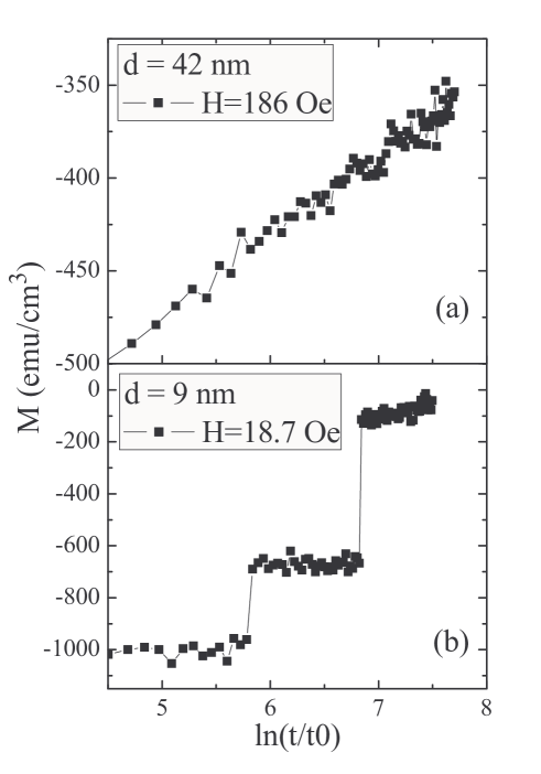
Figure 7: Magnetic relaxation in films of different thickness close to the coercive field. In panel a) we show the behavior of a film of 42 nm, which closely obeys a logarithm law. Panel b) corresponds to a film of 9 nm that presents a discontinuous relaxation.

Magnetic relaxation measurements were also performed in the whole set of samples. For films with $d>28$ nm we found that Eq. 3 is closely obeyed (see Fig. 7 (a)) while in the case of thinner films (9 nm and 19 nm) the relaxation of the magnetization follows a nonlogarithm behavior or occurs in discrete steps, as can be observed in Fig. 7 (b). This last behavior has been only detected for fields very close to $H_{C}$ and is an indication of the very narrow distribution of energy barriers (or switching field distribution) in the thinner films. For the relaxation measurements in these samples we took data every 0.2 Oe which is almost equal to the stability limit (0.1 Oe) of the electromagnet power supply. Possible fluctuations in the applied field can switch the magnetization and it is then difficult to conclude that in this case the reversal of the magnetization is only due to thermal effects. The film with $d=28$ nm was at the limit where a reasonably linear fit could be obtained and was included in the viscosity data, although with a larger uncertainty in the determination of $S$.

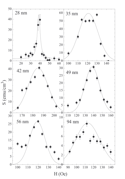
Figure 8: Magnetic viscosity as a function of field in the vicinity of the coercive field. Data are presented for the different samples in which a reasonably linear variation of magnetization with $\ln(t/t_{0})$ was observed. Different sets of data have been fitted with a gaussian distribution from which we extracted $S_{\max}$, $H_{S}$ and $\Delta H_{S}$.

The viscosity parameter, obtained from the slope of curves similar to Fig. 7 (a), is plotted in Fig. 8 for the different films as a function of the applied field. In all cases we observed a maximum value of viscosity, $S_{\max}$, at a field $H_{S}$ which is close, but always smaller, than $H_{C}$ (see Fig. 3). The distribution of viscosity values around $S_{\max}$ has a field width at half maximum height (FWHM) characterized by $\Delta H_{S}$ which is very narrow for $d=28$ nm ($\Delta H_{S}\sim 3$ Oe), increases to an average value $\Delta H_{S}\sim 20$ Oe for $35\leq d\leq 56$ nm and increases again to $\Delta H_{S}\sim 60$ Oe for $d=94$ nm. As already discussed in Section I, the field dependence of $S$ is a measure of the distribution of energy barriers (see Eq. 4) and should correlate closely with the irreversible susceptibility obtained from the derivative of the DCD curves.

In Fig. 9 (a) we present the thickness dependence of the maxima in the magnetic viscosity and the irreversible susceptibility, $S_{\max}$ and $\chi_{irr}^{\max}$, obtained from Figs. 8 and 2, respectively, and in the lower panel of the same figure we can observe the FWHM value of the field distribution of both magnitudes. As expected, the same overall behavior of $S_{\max}$ and $\chi_{irr}^{\max}$ is found for all samples with the exception of $d=28$ nm which has been indicated with an open symbol in Fig. 9 (a). As we already mentioned this film is at the limit in which a logarithm time decay of $M$ is found and, as can be seen in Fig. 8, it has a very narrow field distribution which complicates the precise determination of $S_{\max}$. It is then quite possible that the real value of the maximum viscosity for $d=28$ nm be considerably larger than the reported value, that should then be considered as a lower limit of $S_{\max}.$ Discarding this value of viscosity, it is observed that $S_{\max}$ decreases with film thickness, indicating that the magnetic relaxation in thinner films is faster than in thicker samples. As expected from Eqs. 4 and 5 and observed in Fig. 9 (b) the field distribution of both $S_{\max}$ and $\chi_{irr}^{\max}$ has the same thickness dependence, which indicates that the distribution of activation energies $f(E)$ tends to be considerably narrower for films with $d<d_{cr}$. The sharpness of $\chi_{irr}$ peaks (i.e. smaller $\Delta H\chi_{irr}$ values) has been arguedTomka to be an indication of strong exchange interactions between neighbor grains, consistent with our findings from $\delta M$ curves.

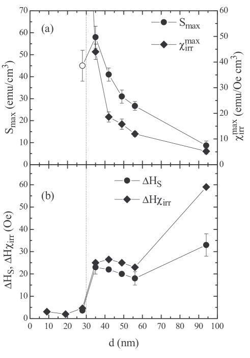
Figure 9: (a) Maximum of the magnetic viscosity and the irreversible susceptibility as a function of film thickness. The open symbol for $d=28$ nm indicates that this sample is at the boundary in which a reasonably linear behavior of $M(t)$ is observed. (b) Field distribution width of both parameters as a function of $d$ (obtained from a gaussian fit of the curves of Fig. 8 and the field derivative of the $m_{d}$ data of Fig. 2). The dotted vertical line indicates the value of $d_{cr}\sim 30$ nm.

III.3
Activation volume and fluctuation field

The activation volume can be calculated from Eq. 6 using the ratio between the maximum values of $S$ and $\chi_{irr}$ or by averaging different values of $V_{ac}(H)$ in the vicinity of the coercive field. To estimate the parameter $c$ entering in Eq. 6 we need to know the reversal mechanism present in our films. We have measured the out of plane angular variation of the coercive field and found that $H_{C}$ increases when the field is applied at increasing angles with respect to the film plane, an indication that reversal is due to the displacement of domain walls. For this case there is a criterion given by GauntGaunt1 for the determination of the pinning regime. He defined a parameter $\beta_{0}=3F/(2\pi\gamma\delta),$ where $F$ is the maximum restoring force a pin can exert on a wall, $\gamma$ is the wall energy and $\delta$ the wall width. For $\beta_{0}<1$ the domain walls are in the weak pinning regime while for $\beta_{0}>1$ the strong pinning situation occurs. A crude estimation for the pinning force is given by $F=1/2(4\pi M_{s}a/3)^{2}$ ($a$ is the radius of the pinning centers or inclusions) and the wall energy can be written as $\gamma=K\delta,$ so that we can write:

$$\beta_{0}=\frac{4\pi M_{s}^{2}}{3K}\left(\frac{a}{\delta}\right)^{2}=\frac{2}{3Q}\left(\frac{a}{\delta}\right)^{2}.$$ (8)

In our films we haveButeraMFM $Q\sim 0.3$ and an average grain size of 4 nm, which may be used as an estimation for the size of the pinning inclusions. The wall width can be obtainedGetzlaff from $\delta=2\sqrt{A/K_{\perp}}\sim 16$ nm ($A\sim 10^{-6}$ erg/cm is the exchange stiffness constantButeraMFM ) giving $\beta_{0}\sim 0.14<1$ for the studied films, which as an indication of weak pinning. We have then used $c=2$ in Eq. 6 and plotted the values of $V_{ac}$ as a function of film thickness in Fig. 10. We can observe that, within the experimental error, there are no significant differences in the two approaches used for calculating $V_{ac}$. Even more, the activation volume seems to be rather constant for the different samples, with an average value $\overline{V_{ac}}=(1.37\pm 0.30)\times 10^{4}$ nm³ which, for spherical volumes, is equivalent to an average activation diameter $\overline{d_{ac}}=30\pm 3$ nm. For the studied samples with $d>d_{cr}$ the activation diameter $\overline{d_{ac}}$ is larger than the grain size, which implies that although the predominant interactions for $d>d_{cr}$ are dipolar-like, there seems to be a positive intergranular exchange coupling which contributes to the collective reversal of volumes larger than the grain size. This is consistent with the fact that the interaction parameter $\alpha$ is positive for $d=35$ nm, the first sample for which the stripe structure is observed, and may also explain the positive ordinate in the $\alpha$ vs. $E_{S}$ curve of Fig. 6. Note also that this value of the activation diameter is of the same order than the film thickness or the stripe half period when $d\gtrsim d_{cr}$, but is much shorter than the stripe length (which is of the order of tens of micrometers), implying that the magnetic volumes that reverse by thermal effects are considerably smaller than the physical volume of the stripes. Our activation diameters are larger than those reported in Refs. [Jeong, ; Luo, ; Pernechele, ] by a factor of two or more (considering that the parameter $c$ appearing in Eq. 6 was taken as $c=1$ in those previously published papers). This is not surprising due to the totally different microstructure between chemically ordered and disordered samples and the larger exchange length in our magnetically soft films.ButeraMFM .

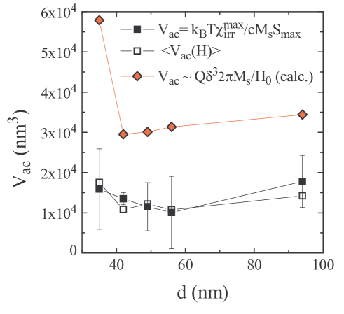
Figure 10: (color online) Activation volume as a function of film thickness. We have calculated $V_{ac}$ from the ratio $\chi_{irr}^{\max}/S_{\max}$ (open squares) and from the average values obtained from measurements at different fields in the vicinity of $H_{C}$ (full squares). The diamond symbols correspond to the calculation of the activation volumes using the model of Gaunt.Gaunt1

The activation volume obtained by the procedure described above may be compared with the theoretical approach in the case of weak domain wall pinning. In this case the activation energy to overcome the barrier depends linearlyGaunt1 ; Gaunt2 on the magnetic field $H,$

$$E_{a}=31\gamma\left(\delta/4\right)^{2}\left(1-H/H_{0}\right),$$ (9)

with $H_{0}$ the pinning field at zero temperature. Since the activation volume is related to the field derivative of the activation energy, we can write

$$V_{ac}=\frac{dE_{a}}{dH}\frac{1}{cM_{s}}=\frac{31\gamma\left(\delta/4\right)^{2}}{H_{0}}\frac{1}{cM_{s}}\sim\frac{Q\delta^{3}2\pi M_{s}}{H_{0}}.$$ (10)

In the last formula we have used $c=2$ and $\gamma=K\delta.$ With this equation it is possible to calculate the activation volume if the coercive field at $T=0$ is known. We have discussed in Ref. [Jonas, ] that at low temperatures there is an unexpected decrease in $H_{C}$ because interface stress effects hinder the formation of stripes, so that a reduction in $H_{C}$ occurs at low temperatures and a value for $H_{0}$ is not experimentally accessible. However, we can still take the maximum value of $H_{C}(T)=H_{C}^{\max}$ as a lower bound estimation for $H_{0}.$ Using the data from Fig. 3 and Eq. 10 we calculated $V_{ac}$ for the set of samples with $d\geq 35$ nm and show the results in Fig. 10. We can observe that the calculated values of $V_{ac}$ are approximately independent of film thickness, with the exception of $d=35$ nm, a case that should be taken with extra care because a maximum in $H_{C}(T)$ was not observed in the studied temperature range. This form of calculating $V_{ac}$ gave in all cases larger values than those obtained using Eq. 6, approximately by a factor of two. The difference may be due to the underestimation of $H_{0}$ or to an overestimation of the wall width $\delta$. Apart from this relatively small discrepancy, the observed experimental behavior is weakly dependent on film thickness, in accordance with the prediction of Eq. 10.

Another experimental procedure for the estimation of the activation volume, which does not need the explicit measurement of $\chi_{irr}$, is the so-called ”waiting time method”.Collocott This method is based on time relaxation measurements of $M$ at different fields close to $H_{S}$, the same curves that are used for the determination of $S(H).$ The model is based on the assumption that both $S$ and $\chi_{irr}$ are relatively constant for fields around $H_{S}.$ When $M(t,H)$ curves are plotted together as a function of $\ln(t/t_{0})$ it can be shown that the following relation is obeyed:

$$\Delta H=H_{f}\,\ln(t_{i}).$$ (11)

If a horizontal line of constant $M$ is drawn, $\Delta H$ represents the field distance between intersection points, and $t_{i}$ the time of intersection. A plot of $\Delta H$ as a function of $\ln(t_{i})$ has a slope $H_{f}$ from which $V_{ac}$ can be obtained using Eq. 7.

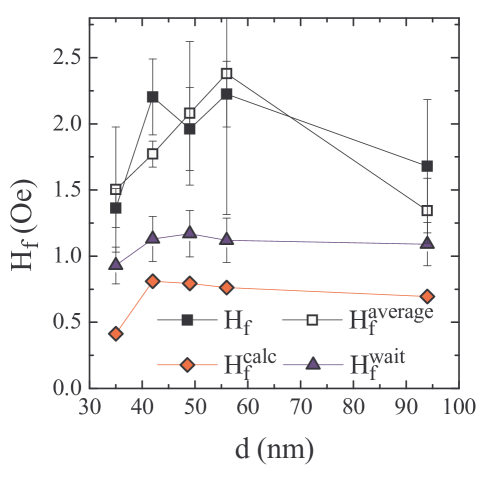
Figure 11: Fluctuation field as a function of film thickness obtained from Fig. 10 and Eq. 7 (squares and diamonds) and from the time relaxation of magnetization at different fields (waiting time method, represented by triangles).

In Fig. 11 we plotted the fluctuation fields obtained from the previously calculated values of $V_{ac}$ and added the data deduced using the waiting time method. Eventhough the error bars are relatively large, it can be seen that these new values of $H_{f}$ are of the same order of magnitude and relatively constant in the studied range of thicknesses, consistent with those previously estimated using the remanence and viscosity measurements. Following Ref. [Wohlfarth, ] we have tried to correlate the values of $H_{f}$ with the coercivity $H_{C}$. According to Wohlfarth there should be a power law relationship between both parameters, $H_{C}\varpropto H_{f}^{x}$, with $x$ in the range 0.5-1 depending on the microstructure and the type of domain wall pinning of the system. Although our data points fall close to those shown in Fig. 1 of Ref. [Wohlfarth, ] it was not possible to fit them using a power law due to the reduced span of the coercivity and the fluctuation field values.

IV Conclusions

We have studied the role of magnetic interactions and thermally activated processes in FePt alloy films as a function of film thickness. We have found that when $d$ is larger than the critical thickness for the formation of a structure of stripes with an antiparallel out of plane component of the magnetization the interactions tend to be dipolar-like, while for $d<d_{cr}$ positive values of $\alpha$ are obtained. This change is probably due to the larger relative weight of the dipolar field present in the films with stripe domains which arrange in a flux closure configuration that tends to favor a demagnetized state. We have found that the large differences between $H_{C}^{\mathrm{rem}}$ and $H_{\mathrm{IRM}}$ are mostly due to the rotational anisotropy generated when the stripe structure is present. The interaction parameter $\alpha$ becomes more negative with increasing thickness which again is a consequence of the predominance of magnetostatic demagnetizing effects for larger values of $d.$ We have shown that this parameter is in close correlation with the surface demagnetizing energy, confirming that dipolar interactions are predominant above the critical thickness. Magnetic viscosity was also found to depend strongly on the domain configuration. In thinner films relaxation seems to occur in discrete steps while for $d>d_{cr}$ the usual logarithm behavior is found. $S(H)$ and $\chi_{irr}(H)$ curves are a good estimation for the distribution of energy barriers and also have a strong variation in the field width depending on the domain structure. We finally estimated the values of the activation volumes that reverse the magnetization assisted by thermal effects and found that they are approximately independent of film thickness. The value of $\overline{d_{ac}}$ is almost an order of magnitude larger than the grain size, evidencing that a relatively large number of grains is coupled by the exchange interaction, but $\overline{d_{ac}}$ is considerably smaller than the length of the stripes (which are several micrometers long), indicating that the reversal occurs in small regions compared to the size of the domains. Different methods of calculating the activation volumes and the fluctuation fields yielded approximately the same results, supporting the procedure used for the estimation of these parameters.

As far as we know, this is the first time that this kind of magnetic measurements have been performed in chemically disordered FePt films in which a transition in the domain structure occurs at a critical thickness. We have clearly evidenced that strong changes in most variables accompany the switch of the magnetic configuration from planar domains to parallel stripes and gave an interpretation of the observed results.

This was supported in part by Conicet under Grant PIP 112-200801-00245, ANPCyT Grant PME # 1070, and U.N. Cuyo Grant 06/C235, all from Argentina. We would like to acknowledge very fruitful discussions with Dr. Emilio de Biasi.

References

- (1) N. Saito, H. Fujiwara, and Y. Sugita, J. Phys. Soc. Japan, 19, 421 (1964).
- (2) M. Hehn, S. Padovani, K. Ounadjela, and J. P. Bucher, Phys. Rev. B 54, 3428 (1996).
- (3) V. Gehanno, R. Hoffmann, Y. Samson, A. Marty, and S. Auffret, Eur. Phys. J. B 10, 457 (1999).
- (4) S. Okamoto, N. Kikuchi, O. Kitakami, T. Miyazaki, Y. Shimada, and K. Fukamichi. Phys. Rev. B 66, 024413(2002).
- (5) E. Sallica Leva, R. C. Valente, F. Martínez Tabares, M. Vásquez Mansilla, S. Roshdestwensky, and A. Butera, Phys. Rev. B 82, 144410 (2010).
- (6) M. Barturen, B. Rache Salles, P. Schio, J. Milano, A. Butera, S. Bustingorry, C. Ramos, A. J. A. de Oliveira, M. Eddrief, E. Lacaze, F. Gendron, V. H. Etgens, and M. Marangolo, Appl. Phys. Lett. 101, 092404 (2012).
- (7) C. Kooy and U. Enz, Philips Res. Rep. 15, 7(1960).
- (8) Y. Murayama, J. Phys. Soc. Jap. 21, 2253 (1966).
- (9) A. L. Sukstanskii and K. I. Primak, J. Magn. Magn. Mat. 169, 31 (1997).
- (10) R. Bručas, H. Hafermann, M. I. Katsnelson, I. L. Soroka, O. Eriksson, and B. Hjörvarsson, Phys. Rev. B, 69, 064411 (2004).
- (11) A. Hubert and R. Schäfer, Magnetic Domains, Springer, 3rd printing (2009).
- (12) M. Vásquez Mansilla, J. Gómez, and A. Butera, IEEE Trans. Magn. 44, 2883 (2008).
- (13) M. Vásquez Mansilla, J. Gómez, E. Sallica Leva, F. Castillo Gamarra, A. Asenjo Barahona, and A. Butera, J. Magn. Magn. Mat. 321, 2941 (2009).
- (14) E. Burgos, E. Sallica Leva, J. Gómez, F. Martínez Tabares, M. Vásquez Mansilla, and A. Butera, Phys. Rev. B 83, 174417 (2011).
- (15) D. M. Jacobi, E. Sallica Leva, N. Álvarez, M. Vásquez Mansilla, J. Gómez and A. Butera, J. Appl. Phys., 111, 033911 (2012).
- (16) J. M. Guzmán, N. Álvarez, H. R. Salva, M. Vásquez Mansilla, J. Gómez, and A. Butera, J. Magn. Magn. Mat. 347, 61 (2013).
- (17) N. Álvarez, G. Alejandro, J. Gómez, E. Goovaerts, and A. Butera. J. Phys. D: Appl Phys. 46, 505001 (2013).
- (18) C.A. Ramos, E. Vassallo Brigneti, J. Gómez, and A. Butera, Physica B 404, 2784 (2009).
- (19) G. W. D. Spratt, P. R. Bissell, R. W. Chantrell, and E. P. Wohlfarth , J. Magn. Magn. Mater. 75, 309 (1988).
- (20) P. E. Kelly, K. O’Grady, P. I. Mayo, and R. W. Chantrell, IEEE Trans. Magn. 25, 3881 (1989).
- (21) J. García Otero, M. Porto, J. Rivas, J. Appl. Phys. 87, 7376 (2000)
- (22) E. P. Wohlfarth, J. Phys. F 14, L155 (1984).
- (23) E. P. Wohlfarth, J. Appl. Phys. 29, 595 (1958).
- (24) X.-d. Che and H. N. Bertram, J. Magn. Magn. Mater. 116, 121 (1992).
- (25) A. Butera and J. A. Barnard in “High-Density Magnetic Recording and Integrated Magneto-Optics: Materials and Devices” Editors: K. Rubin, J.A. Bain, T. Nolan, D. Bogy, B.J.H. Stadler, M. Levy, J.P. Lorenzo, M. Mansuripur, Y.Okamura, R. Wolfe, Materials Research Society (MRS) Symposium Proceedings (San Fransisco, CA, Spring Meeting 1998) Vol.: 517, p. 349 (1998).
- (26) A. Butera, J. L. Weston, and J. A. Barnard, J. Appl. Phys. 81, 7432 (1997). A.Butera, J.L.Weston, and J.A.Barnard, IEEE Trans. Magn. 33, 3604 (1997).
- (27) J. W. Harrell, D. Richards, and M. R. Parker, J. Appl. Phys. 73, 6722 (1993).
- (28) R. Street and J. C. Wooley, Proc. Phys. Soc. London, Sec. A 62, 562 (1949).
- (29) P. Gaunt and G. J. Roy, Philos. Mag. 34, 781 (1976).
- (30) P. Gaunt, J. Appl. Phys. 59, 4129 (1986).
- (31) D. H. L. Ng, C. C. H. Lo, and P. Gaunt, IEEE Trans. Magn. 30, 4854 (1994).
- (32) N. Li, B. M. Lairson, and O.-H. Kwon, J. Magn. Magn. Mat. 205, 1 (1999).
- (33) S. Jeong, M. E. McHenry, and D. Laughlin, IEEE Trans. Magn. 37, 1309 (2001).
- (34) C. P. Luo, Z. S. Shan, and D. J. Sellmyer, J. Appl. Phys. 79, 4899 (1996).
- (35) C. Pernechele, M. Solzi, R. Pellicelli, M. Ghidini, F. Albertini, and F. Casoli, J. Magn. Magn. Mat. 316, e162 (2007).
- (36) D. H. Wei and Y. D. Yao, IEEE Trans. Magn. 45, 4092 (2009).
- (37) D. H. Wei, J. Appl. Phys. J. Appl. Phys. 105, 07A715 (2009).
- (38) Y. Gao, X. W. Zhang, Z. G. Yin, S. Qu, J. B. You, and N. F. Chen, Nanoscale Res. Lett. 5, 1 (2010).
- (39) S. Wang, A. F. Khapikov, S. Brown, and J. W. Harrell, IEEE Trans. Magn. 37, 1518 (2001).
- (40) Physics of Magnetism, S. Chikazumi, Krieger Publishing, Florida (1964).
- (41) G. J. Tomka, P. R. Bissell, K. O’Grady, and R. W. Chantrell, J. Phys. D: Appl. Phys. 27, 1601 (1994).
- (42) Fundamentals of Magnetism, M. Getzlaff, Springer-Verlag, Berlin (2008).
- (43) S. J. Collocott and V. Neu, J. Phys. D: Appl. Phys. 45, 035002 (2012).