On the spacings between the successive zeros of the Laguerre polynomials

Abstract.

We propose a simple uniform lower bound on the spacings between the successive zeros of the Laguerre polynomials $L_{n}^{(\alpha)}$ for all $\alpha>-1$. Our bound is sharp regarding the order of dependency on $n$ and $\alpha$ in various ranges. In particular, we recover the orders given in [1] for $\alpha\in(-1,1]$.

1. Introduction

The study of orthogonal polynomials has a long history with exciting interplay with numerous fields, including random matrix theory. The Laguerre polynomials which occur as the solutions of important differential equations [13], have had many applications in physics (electrostatics, quantum mechanics [6]), engineering (control theory; see e.g. [2]), random matrix theory (Wishart distribution; see e.g. [3] and [5]) and many other fields. The knowledge of the spacings between successive zeros of the Laguerre polynomials, interesting in its own right, is also potentially of great interest in many situations, e.g. for the spacings between successive eigenvalues of Wishart matrices, for bounding the gaps between sucessive energy levels in quantum mechanics or for the analysis of numerical algorithms in system identification problems, to name a few.

In this short note, we provide a uniform lower bound for the gaps between successive zeros of the Laguerre polynomials $L_{n}^{(\alpha)}$. In [1], important bounds were proposed in the case $\alpha\in(-1,1]$ for individual spacings (i.e. bounds depending also on the ranking). Our bound is uniform but it is valid on the entire range $\alpha>-1$. For this reason, our bound might be helpful in a large number of applications. In particular, the cases including large values of $\alpha$, are those of interest for random matrices with Wishart distribution. Our approach is based on a remarkable well known identity (a Bethe ansatz equation; see e.g. [11],[12]).

2. Preliminaries: Bethe ansatz equality

We first recall the following remarkable general result, see e.g. Lemma 1 in [11]. Let $f$ be a polynomial with real simple zeros $x_{1}<\cdots<x_{n}$, satisfying the ODE $f^{\prime\prime}-2af^{\prime}+bf=0$ where $a$ and $b$ are meromorphic function whose poles are different from the $x_{i}$’s. Then for any fixed $k\in\{1\cdots n\}$,

(2.1) $$\sum_{j\neq k}\frac{1}{(x_{k}-x_{j})^{2}} = \frac{\Delta(x_{k})-2a^{\prime}(x_{k})}{3},$$

with $\Delta(x)=b(x)-a^{2}(x)$. Such equalities are called Bethe ansatz equations.

For $\alpha>-1$, the Laguerre polynomials $L_{n}^{(\alpha)}$ ($n$ indicates the degree) are orthogonal polynomials with respect to the weight $x^{\alpha}e^{-x}$ on $(0,\infty)$. Let $x_{n,n}(\alpha)<\cdots<x_{n,1}(\alpha)$ denote the zeros of $L_{n}^{(\alpha)}$. It is known that the polynomial $L_{n}^{(\alpha)}$ is a solution of the second order ODE:

$$u^{\prime\prime}-\left(1-\frac{\alpha+1}{x}\right)u^{\prime}+\frac{n}{x}u = 0.$$

In this case, $a(x)=\frac{1}{2}\left(1-\frac{\alpha+1}{x}\right)$. Therefore,

$$\Delta(x)=\frac{n}{x}-\frac{(x-\alpha-1)^{2}}{4x^{2}}=\frac{-x^{2}+(2(\alpha+1)+4n)x-(\alpha+1)^{2}}{4x^{2}},$$

and then using the notations in [11],

(2.2) $$\Delta(x) = \frac{(U^{2}-x)(x-V^{2})}{4x^{2}},$$

where

(2.3) $$U=\sqrt{n+\alpha+1}+\sqrt{n},\quad V=\sqrt{n+\alpha+1}-\sqrt{n}.$$

Since the l.h.s. of (2.1) is positive and $a^{\prime}(x)>0$ for $x>0$, an immediate consequence of (2.1) is that for all $k$, $(U^{2}-x_{n,k}(\alpha))(x_{n,k}(\alpha)-V^{2})>0$, i.e.

(2.4) $$V^{2}<x_{n,n}(\alpha)<x_{n,1}(\alpha)<U^{2}.$$

Several bounds for the extreme zeros are known and can be found in [4, 7, 10, 11, 13]. For instance, using the Bethe ansatz, Krasikov proved [11, Theorem 1]:

(2.5) $$V^{2}+3V^{4/3}(U^{2}-V^{2})^{-1/3}\leq x_{n,n}(\alpha)<x_{n,1}(\alpha)\leq U^{2}-3U^{4/3}(U^{2}-V^{2})^{-1/3}+2.$$

3. Main result

We show by means of elementary computations that the Bethe ansatz equality actually yields a simple uniform lower bound for $x_{n,k}(\alpha)-x_{n,k+1}(\alpha)$, which turns out to be sharp, see Remark (2) below.

Theorem 3.1.

Let $\alpha>-1$. Then, the following lower bound for the spacings holds for all $k\in\{1,\cdots,n-1\}$:

(3.6) $$x_{n,k}(\alpha)-x_{n,k+1}(\alpha) \geq \sqrt{3}\frac{\alpha+1}{\sqrt{n(n+\alpha+1)}}.$$

Moreover, if $\alpha\geq n/C$ for some $C>0$, we have

(3.7) $$x_{n,k}(\alpha)-x_{n,k+1}(\alpha) \geq \frac{1}{\sqrt{C+1}}\sqrt{\frac{\alpha}{n}}.$$

3.1. Proof of Theorem 3.1

From (2.1), (2.4) and $a^{\prime}(x)>0$ for $x>0$, we deduce the following inequality

(3.8) $$\frac{1}{(x_{n,k}(\alpha)-x_{n,k+1}(\alpha))^{2}}\leq\sum_{j\neq k}\frac{1}{(x_{n,k}(\alpha)-x_{n,j}(\alpha))^{2}}\leq\frac{1}{3}\sup_{V^{2}\leq x\leq U^{2}}\Delta(x).$$

The first inequality above seems to be crude, but is not, see Remark (1) below.

Let us then study the function $\Delta$. The derivative of $\Delta$ on $(0,+\infty)$ reads:

$$\Delta^{\prime}(x)=\frac{(-2x+U^{2}+V^{2})x^{2}-2x\left(-x^{2}+(U^{2}+V^{2})x-U^{2}V^{2}\right)}{4x^{4}}=\frac{2U^{2}V^{2}-(U^{2}+V^{2})x}{4x^{3}}.$$

Thus, $\Delta$ has a unique maximum on $(0,+\infty)$ that is reached at $x^{*}=\frac{2U^{2}V^{2}}{U^{2}+V^{2}}$. We have:

$$U^{2}-x^{*} = \frac{U^{4}-U^{2}V^{2}}{U^{2}+V^{2}}=U^{2}\frac{U^{2}-V^{2}}{U^{2}+V^{2}}$$

$$x^{*}-V^{2} = \frac{U^{2}V^{2}-V^{4}}{U^{2}+V^{2}}=V^{2}\frac{U^{2}-V^{2}}{U^{2}+V^{2}}.$$

Thus, we obtain by plugging into (2.2),

$$\sup_{V^{2}\leq x\leq U^{2}}\Delta(x)=\Delta(x^{*})=\frac{(U^{2}-V^{2})^{2}}{16\ U^{2}V^{2}},$$

since one can check that $x^{*}\in(V^{2},U^{2})$. Moreover, from the expressions (2.3) of $U$ and $V$:

$$U^{2}-V^{2} = (U-V)(U+V)=4\sqrt{n}\sqrt{n+\alpha+1}$$

$$UV = \alpha+1.$$

Hence, plugging these last equalities in (3.8), we can write

$$\frac{1}{(x_{n,k}(\alpha)-x_{n,k+1}(\alpha))^{2}} \leq \frac{1}{3}\ \frac{4^{2}\ n(n+\alpha+1)}{16\ (\alpha+1)^{2}},$$

and finally

$$x_{n,k}(\alpha)-x_{n,k+1}(\alpha) \geq \sqrt{3}\frac{\alpha+1}{\sqrt{n(n+\alpha+1)}}.$$

Now assume that $n\leq C\alpha$. Then $n+\alpha+1\leq(C+1)\alpha+1$. Therefore $\sqrt{n+\alpha+1}\leq\sqrt{2(C+1)\alpha}$, where we used $1\leq C\alpha\leq(C+1)\alpha$. Hence

$$x_{n,k}(\alpha)-x_{n,k+1}(\alpha) \geq \sqrt{\frac{3}{2(C+1)}}\sqrt{\frac{\alpha}{n}},$$

which completes the proof of Theorem 3.1.

3.2. Remarks

1. Notice that replacing the sum $\sum_{j\neq k}(x_{n,k}(\alpha)-x_{n,j}(\alpha))^{-2}$ by the single term $(x_{n,k}(\alpha)-x_{n,k+1}(\alpha))^{-2}$ does not deteriorate a priori the order of dependency on $n$ and $\alpha$ of a uniform bound in $k$ of $x_{n,k}(\alpha)-x_{n,k+1}(\alpha)$. Indeed, let $0<\delta<x_{n,k}(\alpha)-x_{n,k+1}(\alpha)$ for all $k$, we have the following simple inequality for any fixed $k$:

   $$\frac{1}{(x_{n,k}(\alpha)-x_{n,k+1}(\alpha))^{2}}\leq\sum_{j\neq k}\frac{1}{(x_{n,k}(\alpha)-x_{n,j}(\alpha))^{2}}\leq\sum_{j\neq k}\frac{1}{(\delta|j-k|)^{2}}\leq 2\frac{\pi^{2}}{6}\ \frac{1}{\delta^{2}}.$$

2. Let us verify that our bound is sharp regarding the order of dependency on $n$ and $\alpha$ in various ranges.
   Case $\alpha\in(-1,1]$: Theorem 5.1 in [1] says that for all $\alpha\in(-1,1]$:

   $$\left(n+(\alpha+1)/2\right)\left(x_{n,k}(\alpha)-x_{n,k+1}(\alpha)\right) \xrightarrow[]{n\to\infty} j_{\alpha,k+1}^{2}-j_{\alpha,k}^{2},$$

   where $j_{\alpha,k}$ is the $k$-th zeros of the Bessel function $J_{\alpha}(x)$. But, for all $k\geq 1$, the following holds (see [8, Theorem 3] and [9, p.2]):

   $$\pi\leq j_{\alpha,k+1}-j_{\alpha,k}\leq 2\pi$$

   $$j_{\alpha,k+1}+j_{\alpha,k}\geq 2\sqrt{(k-1/4)^{2}\pi+\alpha^{2}}\geq 1+\alpha.$$

   As a consequence, for small $k$, $x_{n,k}(\alpha)-x_{n,k+1}(\alpha)\sim C(\alpha)/n$, which is consistent with our bound (3.6).
   Case $n\leq C\alpha$ for an absolute constant $C>0$: Summing (3.7) over $k$ yields

   $$\frac{\sqrt{n\alpha}}{\sqrt{C+1}} \leq \sum_{1\leq k\leq n-1}\left(x_{n,k}(\alpha)-x_{n,k+1}(\alpha)\right)=x_{n,1}(\alpha)-x_{n,n}(\alpha)$$

   $$\leq U^{2}-V^{2}=4\sqrt{n}\sqrt{n+\alpha+1}\leq 6\sqrt{C+1}\sqrt{n\alpha},$$

   which means that the bound (3.7) is sharp with respect to the orders of $n$ and $\alpha$ up to a multiplicative constant.

   Notice moreover that in full generality, $C$ can be taken as a function of $n$ with absolutely no change in the proof.

3. Finally, since the Bethe ansatz equation (2.1) is a general equality for polynomials $f$ with real simple zeros, satisfying the ODE $f^{\prime\prime}-2af^{\prime}+bf=0$, good prior bounds on the extreme zeros for such polynomials could be used to obtain similar results as Theorem 3.1.

4. Numerical results

We now provide numerical results on the successive spacings of the Laguerre polynomials $L_{n}^{(\alpha)}$ for various values of $n$ and $\alpha$.

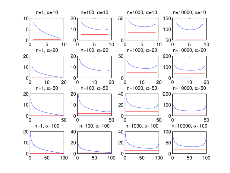
Figure 1. Comparison between the uniform bound (3.6) in red, and the function $i\mapsto x_{n,i}(\alpha)-x_{n,i+1}(\alpha)$, $1\leq i\leq n-1$, in blue. We set $\alpha=1,100,10^{3},10^{4}$ and $n=10,20,50,100$.

Let us make a few comments on Figure 1. The first column illustrates that the uniform bound almost coincides with the smallest spacing, which is here $x_{n,n-1}(1)-x_{n,n}(1)$ (Recall that $x_{n,n}(\alpha)$ is the smallest zero). When $\alpha$ is large compared to $n$, the behavior is quite different. For instance, based on Remark 2 in the case $\alpha\geq n/C$, we can expect most spacings to be almost equal, i.e. close to the uniform lower bound $\sqrt{\alpha/n}$ up to a multiplicative constant. In the last two columns of Figure 1 (large values of $\alpha$ compared to $n$), we observe that this phenomena actually occurs in the bulk, i.e. for $\varepsilon n\leq i\leq(1-\varepsilon)n$, $0<\varepsilon<1$.

The results plotted in Figure 1 have been obtained using Matlab and the codes available at http://people.sc.fsu.edu/~jburkardt/m_src/laguerre_polynomial/.

References

• [1] Ahmed, S., Laforgia, A. and Muldoon, M. E. On the spacing of the zeros of some classical orthogonal polynomials. J. London Math. Soc. (2) 25 (1982), no. 2, 246–252.
• [2] Datta, Kanti B. and Mohan, B. M. Orthogonal functions in systems and control. Advanced Series in Electrical and Computer Engineering, 9. World Scientific Publishing Co., Inc., River Edge, NJ, 1995.
• [3] Dette, H. and Imhof, L., Uniform approximation of eigenvalues in Laguerre and Hermite $\beta$- ensembles by roots of orthogonal polynomials, Transactions of the AMS, 359 (2007), 10, 4999-5018.
• [4] Dimitrov, D. K. and Nikolov, G. P Sharp bounds for the extreme zeros of classical orthogonal polynomials. J. Approx. Theory 162 (2010), no. 10, 1793–1804.
• [5] Faraut, J., Logarithmic Potential Theory, Orthogonal Polynomials, and Random Matrices CIMPA School, Hammamet, September 2011. Lecture notes available at http://www.math.jussieu.fr/ faraut/CIMPA-2011-JF.pdf.
• [6] Freeden, Willi and Gutting, Martin, Special functions of mathematical (geo-)physics. Applied and Numerical Harmonic Analysis. Birkhäuser/Springer Basel AG, Basel, 2013.
• [7] Gatteschi, L. Asymptotics and bounds for the zeros of Laguerre polynomials: a survey. J. Comput. Appl. Math. 144 (2002), no. 1-2, 7–27.
• [8] Hethcote, H.W. Bounds for zeros of some special functions, Proc. Amer. Math. Soc. 25 (1970), 72-74.
• [9] Finch, S. http://www.people.fas.harvard.edu/ sfinch/csolve/bs.pdf
• [10] Ismail, Mourad E. H. and Li, X. Bound on the extreme zeros of orthogonal polynomials. Proc. Amer. Math. Soc. 115 (1992), no. 1, 131–140.
• [11] Krasikov, I. On extreme zeros of classical orthogonal polynomials. J. Comput. Appl. Math. 193 (2006), no. 1, 168–182.
• [12] Krasovsky, I. V., Asymptotic distribution of zeros of polynomials satisfying difference equations. J. Comput. Appl. Math. 150 (2003), no. 1, 56–70.
• [13] Szego, G., Orthogonal polynomials, AMS (1975).
• [14] R. Vershynin, Introduction to the non-asymptotic analysis of random matrices. Compressed sensing, 210–268, Cambridge Univ. Press, Cambridge, 2012.