Rayleigh-Taylor instabilities with sheared magnetic fields

Abstract

Magnetic Rayleigh-Taylor (MRT) instabilities may play a relevant role in many astrophysical problems. In this work the effect of magnetic shear on the growth rate of the MRT instability is investigated. The eigenmodes of an interface and a slab model under the presence of gravity are analytically calculated assuming that the orientation of the magnetic field changes in the equilibrium, i.e., there is magnetic shear. We solve the linearised magnetohydrodynamic (MHD) equations in the incompressible regime.We find that the growth rate is bounded under the presence of magnetic shear. We have derived simple analytical expressions for the maximum growth rate, corresponding to the most unstable mode of the system. These expressions provide the explicit dependence of the growth rate on the various equilibrium parameters. For small angles the growth time is linearly proportional to the shear angle, and in this regime the single interface problem and the slab problem tend to the same result. On the contrary, in the limit of large angles and for the interface problem the growth time is essentially independent of the shear angle. In this regime we have also been able to calculate an approximate expression for the growth time for the slab configuration. Magnetic shear can have a strong effect on the growth rates of the instability. As an application of the results found in this paper we have indirectly determined the shear angle in solar prominence threads using their lifetimes and the estimation of the Alfvén speed of the structure.

1. Introduction

The magnetic Rayleigh-Taylor (MRT) instability is important in many astrophysical systems. Some examples are buoyant magnetised bubbles identified in clusters of galaxies, see Robinson et al. (2004); Jones & De Young (2005) for studies in 2D, and O’Neill et al. (2009) for 3D configurations. MRT instabilities also manifest themselves in shells of young supernova remnants, this has been investigated by Jun et al. (1995) in 2 and 3D Cartesian configurations and by Jun & Norman (1996) in 3D using spherical coordinates. Bucciantini et al. (2004) have numerically investigated the development of the MRT instability at the interface between an expanding pulsar wind nebula and its surrounding supernova remnant. Stone & Gardiner (2007) studied the behaviour of magnetic Rayleigh-Taylor instability in three dimensions with special focus on the structure and dynamics of the nonlinear evolution of the system. They analysed various configurations including the situation in which magnetic fields change direction at the interface between the two fluids. Stone & Gardiner (2007) used the MRT instability to explain the structure of the optical filaments observed in the Crab nebula.

In laboratory plasmas the possible stabilising effect by a force-free magnetic field has been studied in the past by many authors (see for example Goedbloed, 1971a, b, c; Goedbloed & Poedts, 2004) using the single interface problem and the slab problem and applying vacuum conditions at some of the boundaries. Yang et al. (2011) have studied the magnetic field transition layer effects on the MRT instability with continuous magnetic field and density profiles and have found that the linear growth rate of the MRT instability increases with the thickness of the magnetic field transition layer, especially for the case of small thickness. Recently, Zhang et al. (2012) have used the ideal MHD model to study the effect of magnetic shear in a finite slab representing a magnetic liner, which is a device used in experiments with fusion plasmas. These authors have found that magnetic shear reduces the MRT growth rate in general.

The emergence of magnetic flux from the solar interior and the formation of flux tubes is another example where MRT instabilities are relevant. For example, Isobe et al. (2005, 2006) proposed that the MRT instability is a possible cause of the filamentary structure in mass and current density in the emerging flux regions. In the solar atmosphere, Ryutova et al. (2010) suggested that several dynamic processes taking place in prominences are most probably related to magnetic Rayleigh-Taylor instabilities. Along this line of work, Hillier et al. (2011, 2012a, 2012b) have performed three-dimensional magnetohydrodynamic simulations to investigate the nonlinear evolution of the Kippenhahn-Shlüter prominence model to the MRT instability.

The fine structure of solar prominences reveals the presence of magnetic threads. These structures are quite thin, of the order of $100\,\rm km$, aligned with the magnetic field and, in many cases, they seem to lie horizontally with respect to the photosphere (see DeVore, 2012, 2013, for recent results about the formation of these structures). Terradas et al. (2012) have considered the possible link between magnetic Rayleigh-Taylor instabilities and the short thread lifetimes. In that work a slab model permeated by a horizontal magnetic field was considered. The growth rates of the unstable modes and the thresholds for stability were determined analytically. In the present paper we extend the study to the situation with a sheared magnetic field in which the magnetic field changes its direction at the interfaces of the plasma slab. To understand the results in the slab model we describe first the effect of shear at a single plasma interface. Magnetic shear introduces changes in the growth rates of the unstable modes that might be relevant regarding the lifetime of threads. In this work we analytically calculate these growth rates and perform a detailed analysis of their dependence on the equilibrium parameters.

2. Problem formulation

To describe the plasma motion we use the linearised ideal MHD equation for incompressible plasmas

$$\nabla\cdot\boldsymbol{\xi}=0,$$ (1)

$$\rho\frac{\partial^{2}\boldsymbol{\xi}}{\partial t^{2}}=-\nabla p+\frac{1}{\mu_{0}}(\nabla\times\boldsymbol{b})\times\boldsymbol{B},$$ (2)

$$\boldsymbol{b}=\nabla\times(\boldsymbol{\xi}\times\boldsymbol{B}).$$ (3)

Here $\boldsymbol{\xi}$ is the plasma displacement related to the plasma velocity $\boldsymbol{u}$ by $\boldsymbol{u}=\partial\boldsymbol{\xi}/\partial t$, $p$ the pressure perturbation, and $\boldsymbol{b}$ the magnetic field perturbation; $\boldsymbol{B}$ is the background magnetic field, $\rho$ the plasma density assumed to be piecewise constant, and $\mu_{0}$ the magnetic permeability of free space. When deriving Eqs. (1)–(3) we have assumed that the equilibrium is static and current-free, e.g. $\nabla\times\boldsymbol{B}=0$.

In what follows we consider two equilibrium states. In the first one there are two semi-infinite regions separated by the $xy$-plane in Cartesian coordinates $x$, $y$, $z$ with the $z$-axis in the vertical direction, see Fig. 1. The plasma density and background magnetic field are constant in the two regions and they are given by

$$\rho=\left\{\begin{array}[]{ll}\rho_{e},&z<0,\\ \rho_{i},&z>0,\end{array}\right.\quad\boldsymbol{B}=\left\{\begin{array}[]{ll}\boldsymbol{B}_{e},&z<0,\\ \boldsymbol{B}_{i},&z>0.\end{array}\right.$$ (4)

The background magnetic field is assumed to be parallel to the $xy$-plane. The equilibrium pressure $P$ is defined by the equation

$$\frac{dP}{dz}=-g\rho,$$ (5)

where $g$ is the gravity acceleration. The total pressure, magnetic plus kinetic, has to be continuous at $z=0$. The solution to Eq. (5) satisfying this condition is

$$P=\left\{\begin{array}[]{ll}\displaystyle P_{0}-\frac{B_{e}^{2}}{2\mu_{0}}-g\rho_{e}z,&z<0,\vspace*{2mm}\\ \displaystyle P_{0}-\frac{B_{i}^{2}}{2\mu_{0}}-g\rho_{i}z,&z>0,\end{array}\right.$$ (6)

where $P_{0}$ is an arbitrary constant. We call this equilibrium state the single magnetic interface.

Figure 1.— Sketch of single magnetic interface.

In the second equilibrium state there are three regions separated by horizontal planes at $z=\pm a$, see Fig. 2. The plasma density and background magnetic field are the same in two semi-infinite regions and they are given by

$$\rho=\left\{\begin{array}[]{ll}\rho_{e},&z<-a,\\ \rho_{i},&|z|<a,\\ \rho_{e},&z>a,\end{array}\right.\quad\boldsymbol{B}=\left\{\begin{array}[]{ll}\boldsymbol{B}_{e},&z<-a,\\ \boldsymbol{B}_{i},&|z|<a,\\ \boldsymbol{B}_{e},&z>a.\end{array}\right.$$ (7)

The background magnetic field is once again assumed to be parallel to the $xy$-plane. The total pressure has to be continuous at $z=\pm a$. The solution to Eq. (5) satisfying this condition is

$$P=\left\{\begin{array}[]{ll}\displaystyle P_{0}-\frac{B_{e}^{2}}{2\mu_{0}}\,+\,ga(\rho_{i}-\rho_{e})-g\rho_{e}z,&z<-a,\vspace*{2mm}\\ \displaystyle P_{0}-\frac{B_{i}^{2}}{2\mu_{0}}-g\rho_{i}z,&|z|<a,\vspace*{2mm}\\ \displaystyle P_{0}-\frac{B_{e}^{2}}{2\mu_{0}}\,-\,ga(\rho_{i}-\rho_{e})-g\rho_{e}z,&z>a.\end{array}\right.$$ (8)

This second configuration is called the magnetic slab.

Figure 2.— Sketch of magnetic slab.

At the boundaries separating regions with different plasma densities and background magnetic field the plasma displacement in the $z$-direction and the Lagrangian perturbation of the total pressure have to be continuous. Hence, we have two boundary conditions,

$$[\,\xi_{z}\,]=0,\quad[\,p_{T}-g\rho\xi_{z}\,]=0,$$ (9)

where the square brackets denote the jump of a quantity across a discontinuity, and $p_{T}=p+\boldsymbol{B}\cdot\boldsymbol{b}/\mu_{0}$ is the perturbation of the total pressure. When deriving the second boundary condition we have used Eq. (5). The boundary conditions (9) have to be satisfied at $z=0$ in the case of the single magnetic interface, and at $z=\pm a$ in the case of the magnetic slab. One additional boundary condition is that all perturbations have to vanish as $|z|\to\infty$.

Equations (1)–(3) together with the boundary conditions (9) are used in the next section to derive the dispersion relations determining the stability of the two equilibrium configurations.

3. Derivation of the dispersion relations

We Fourier-analyse the perturbations of all quantities and take them proportional to $\exp[i(\boldsymbol{k}\cdot\boldsymbol{r}-\omega t)]$, where $\boldsymbol{k}=(k_{x},k_{y},0)$ and $\boldsymbol{r}=(x,y,z)$. Then Eqs. (1)–(3) reduce to

$$\frac{d\xi_{z}}{dz}+i\boldsymbol{k}\cdot\boldsymbol{\xi}=0,$$ (10)

$$\rho\omega^{2}\boldsymbol{\xi}_{\perp}=i\boldsymbol{k}p_{T}-\frac{i}{\mu_{0}}\boldsymbol{b}_{\perp}(\boldsymbol{k}\cdot\boldsymbol{B}),$$ (11)

$$\rho\omega^{2}\xi_{z}=\frac{dp_{T}}{dz}-\frac{i}{\mu_{0}}b_{z}(\boldsymbol{k}\cdot\boldsymbol{B}),$$ (12)

$$\boldsymbol{b}=i(\boldsymbol{k}\cdot\boldsymbol{B})\boldsymbol{\xi},$$ (13)

where $\boldsymbol{\xi}_{\perp}$ and $\boldsymbol{b}_{\perp}$ are the components of the plasma displacement and magnetic field perturbation orthogonal to the $z$-axis. Eliminating all the variables from Eqs. (10)–(13) in favour of $\xi_{z}$ we obtain the equation for this variable,

$$\frac{d^{2}\xi_{z}}{dz^{2}}-k^{2}\xi_{z}=0.$$ (14)

In addition, we obtain the expression of $p_{T}$ in terms of $\xi_{z}$,

$$p_{T}=\frac{\rho(\omega^{2}-\omega_{A}^{2})}{k^{2}}\frac{d\xi_{z}}{dz},$$ (15)

where $\omega_{A}$ is the Alfvén frequency defined by

$$\omega_{A}^{2}=\frac{(\boldsymbol{k}\cdot\boldsymbol{B})^{2}}{\mu_{0}\rho}.$$ (16)

This expression enables us to rewrite the boundary conditions (9) in terms of $\xi_{z}$ as

$$[\,\xi_{z}\,]=0,\quad\left[\rho(\omega^{2}-\omega_{A}^{2})\frac{d\xi_{z}}{dz}-g\rho k^{2}\xi_{z}\right]=0.$$ (17)

3.1. Dispersion relation for a single magnetic interface

In the case of a single magnetic interface the solution to Eq. (14), satisfying the first boundary condition in Eq. (17) at $z=0$ and decaying as $|z|\to\infty$, is given, with the accuracy up to an arbitrary multiplicative constant, by

$$\xi_{z}=\left\{\begin{array}[]{ll}e^{kz},&z<0,\vspace*{1mm}\\ e^{-kz},&z>0.\end{array}\right.$$ (18)

Substituting this solution in the second boundary condition in Eq. (17) we obtain the following dispersion relation

$$\omega^{2}=\frac{\rho_{e}\omega_{Ae}^{2}+\rho_{i}\omega_{Ai}^{2}+gk(\rho_{e}-\rho_{i})}{\rho_{e}+\rho_{i}}.$$ (19)

This is the well-known dispersion equation for the interface problem in an incompressible fluid (Chandrasekhar, 1961). When $g=0$ this is the dispersion equation for surface waves on a magnetic interface (e.g. Roberts, 1981a). On the other hand, when there is no magnetic field, this dispersion equation determines the Rayleigh-Taylor instability of the interface between two incompressible fluids (Rayleigh, 1883; Taylor, 1950).

3.2. Dispersion relation for the magnetic slab

Now we proceed to the derivation of the dispersion equation for the magnetic slab. The general solution to Eq. (14) continuous at $z=\pm a$ and decaying as $|z|\to\infty$ is

$$\xi_{z}=\left\{\begin{array}[]{ll}\left[C_{1}\cosh(ka)-C_{2}\sinh(ka)\right]e^{k(z+a)},&z<-a,\vspace*{1.5mm}\\ \hphantom{[}C_{1}\cosh(kz)+C_{2}\sinh(kz),&|z|<a,\vspace*{1.5mm}\\ \left[C_{1}\cosh(ka)+C_{2}\sinh(ka)\right]e^{-k(z-a)},&z>a,\end{array}\right.$$ (20)

where $C_{1}$ and $C_{2}$ are arbitrary constants. Substituting this solution in the second boundary condition in Eq. (17) we obtain two equations,

$$A_{11}C_{1}-A_{12}C_{2}=0,\quad A_{21}C_{1}+A_{22}C_{2}=0,$$ (21)

where

$$\begin{array}[]{l}A_{11}=\rho_{e}(\omega^{2}-\omega_{Ae}^{2})+gk(\rho_{i}-\rho_{e})\vspace*{1.5mm}\\ \hskip 91.04881pt+\,\rho_{i}(\omega^{2}-\omega_{Ai}^{2})\tanh(ka),\vspace*{1.5mm}\\ A_{12}=\big{[}\rho_{e}(\omega^{2}-\omega_{Ae}^{2})+gk(\rho_{i}-\rho_{e})\big{]}\tanh(ka)\vspace*{1.5mm}\\ \hskip 130.88268pt+\,\rho_{i}(\omega^{2}-\omega_{Ai}^{2}),\vspace*{1.5mm}\\ A_{21}=\rho_{e}(\omega^{2}-\omega_{Ae}^{2})-gk(\rho_{i}-\rho_{e})\vspace*{1.5mm}\\ \hskip 91.04881pt+\,\rho_{i}(\omega^{2}-\omega_{Ai}^{2})\tanh(ka),\vspace*{1.5mm}\\ A_{22}=\big{[}\rho_{e}(\omega^{2}-\omega_{Ae}^{2})-gk(\rho_{i}-\rho_{e})\big{]}\tanh(ka)\vspace*{1.5mm}\\ \hskip 130.88268pt+\,\rho_{i}(\omega^{2}-\omega_{Ai}^{2}).\end{array}$$ (22)

The system (21) of linear homogeneous equations for $C_{1}$ and $C_{2}$ has non-trivial solutions when its determinant is zero. This condition is written as $A_{11}A_{22}+A_{12}A_{21}=0$. After some algebra this equation gives

$$\omega^{4}\big{[}2\rho_{e}\rho_{i}+\big{(}\rho_{e}^{2}+\rho_{i}^{2}\big{)}\tanh(2ka)\big{]}-2\omega^{2}\big{[}\rho_{e}\rho_{i}\big{(}\omega_{Ae}^{2}\hphantom{xxx}$$

$$\hphantom{xx}+\,\omega_{Ai}^{2}\big{)}+\big{(}\rho_{e}^{2}\omega_{Ae}^{2}+\rho_{i}^{2}\omega_{Ai}^{2}\big{)}\tanh(2ak)\big{]}$$

$$\hphantom{xx}+\,2\rho_{e}\rho_{i}\omega_{Ae}^{2}\omega_{Ai}^{2}+\big{(}\rho_{e}^{2}\omega_{Ae}^{4}+\rho_{i}^{2}\omega_{Ai}^{4}\big{)}\tanh(2ak)$$

$$\hphantom{xx}-\,g^{2}k^{2}(\rho_{e}-\rho_{i})^{2}\tanh(2ak)=0.$$ (23)

The two solutions to this dispersion equation are $\omega_{+}^{2}$ and $\omega_{-}^{2}$ given by

$$\omega_{\pm}^{2}=\frac{F\pm G}{H},$$ (24)

where

$$F = \rho_{i}\rho_{e}\big{(}\omega_{Ai}^{2}+\omega_{Ae}^{2}\big{)}\cosh(2ka)$$ (25)

$$+ \big{(}\rho_{i}^{2}\omega_{Ai}^{2}+\rho_{e}^{2}\omega_{Ae}^{2}\big{)}\sinh(2ka),$$

$$G = \Big{\{}\rho_{i}^{2}\rho_{e}^{2}(\omega_{Ai}^{2}-\omega_{Ae}^{2})^{2}+g^{2}k^{2}(\rho_{i}-\rho_{e})^{2}$$ (26)

$$\times \big{[}\big{(}\rho_{i}^{2}+\rho_{e}^{2}\big{)}\sinh^{2}(2ka)+\rho_{i}\rho_{e}\sinh(4ka)\big{]}\Big{\}}^{1/2},\hphantom{xx}$$

$$H=2\rho_{i}\rho_{e}\cosh(2ka)+\big{(}\rho_{i}^{2}+\rho_{e}^{2}\big{)}\sinh(2ka).$$ (27)

When $g=0$ the dispersion relation given by Eq. (24) describes waves in a magnetic slab (e.g. Parker, 1974; Edwin & Roberts, 1982). The plus sign corresponds to kink waves where $\xi_{z}(z)$ is an even function of $z$, while the minus sign corresponds to sausage waves where $\xi_{z}(z)$ is an odd function of $z$. Although, when $g\neq 0$, $\xi_{z}(z)$ is neither odd nor even in both perturbation modes described by Eq. (24), we will still use the name “kink” for modes with the plus sign, and “sausage” for modes with the minus sign. It can be also shown that Eq. (24) in the absence of magnetic shear reduces to Eq. (22) in Terradas et al. (2012).

4. Investigation of stability

Here we use the dispersion equations derived in the previous section to study the stability of a single magnetic interface and a magnetic slab.

4.1. Stability of a single magnetic interface

Without loss of generality we can choose the $x$-axis in the direction of the vector $\boldsymbol{B}_{i}$. It is convenient to introduce the angle $\varphi$ between the $x$-axis and the wave vector $\boldsymbol{k}$. Then we write $\boldsymbol{k}=k(\cos\varphi,\sin\varphi,0)$, and we also introduce the angle $\alpha$ between $\boldsymbol{B}_{e}$ and $\boldsymbol{B}_{i}$, so $\boldsymbol{B}_{e}=B_{e}(\cos\alpha,\sin\alpha,0)$. Since the MHD equations are invariant under the substitution $-\boldsymbol{B}$ for $\boldsymbol{B}$, we can always choose such the direction of vector $\boldsymbol{B}_{e}$ that the angle $\alpha$ is either acute or right. Hence, in what follows we assume that $0\leq\alpha\leq\pi/2$. Finally, we introduce the dimensionless parameters $\zeta=\rho_{i}/\rho_{e}$ and $\chi=B_{i}/B_{e}$. We rewrite Eq. (19) as

$$\omega^{2}=\frac{g^{2}h}{V_{Ae}^{2}}\frac{h\big{[}\chi^{2}\cos^{2}\varphi+\cos^{2}(\varphi-\alpha)\big{]}+1-\zeta}{\zeta+1},$$ (28)

where the Alfvén speed in the lower medium, $V_{Ae}$, and the dimensionless wave number $h$ are defined by

$$V_{Ae}^{2}=\frac{B_{e}^{2}}{\mu_{0}\rho_{e}},\quad h=\frac{V_{Ae}^{2}k}{g}.$$ (29)

A well-known result is that the interface is stable when $\zeta<1$, i.e. when the density of the upper medium is smaller than that of the lower medium. In the opposite situation, i.e. when $\zeta>1$, there is a qualitative difference between the case where the magnetic field is in the same direction at the two sides of the interface ($\alpha=0$), and the case where the magnetic field is sheared ($\alpha\neq 0$). In the first case perturbations with the wave vector perpendicular to the magnetic field ($\varphi=\pi/2$) are unstable for any value of the dimensionless wave number $h$. Since, for such perturbations, the instability increment or growth rate is equal to

$$\sqrt{gk\frac{\zeta-1}{\zeta+1}},$$

the instability growth rate is unbounded. This means that the initial value problem describing the evolution of the interface initial perturbation is ill-posed. Of course, the growth rate will be bounded and the problem will be well-posed if we take into account either dissipation or the finite thickness of the transition between the two homogeneous regions.

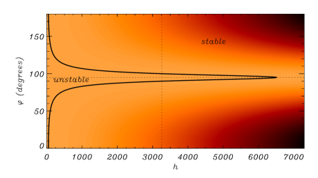
Figure 3.— Square of the frequency (in arbitrary units) as a function of the dimensionless number $h$ and $\varphi$ for the interface. The continuous curve corresponds to $\omega=0$ and represents the transition between stable and unstable modes. The horizontal and vertical dotted lines, respectively, represent the critical angle $\varphi_{c}$, and the wave number $\bar{h}_{c}/2$ at which the increment takes its maximum value. In this plot, $\alpha=10^{\circ}$, $\chi=1$, and $\zeta=100$.

In the second case ($\alpha\neq 0$) perturbations with a fixed direction of the wave number defined by the angle $\varphi$ are unstable only when

$$h<h_{c}(\varphi)=\frac{\zeta-1}{\chi^{2}\cos^{2}\varphi+\cos^{2}(\varphi-\alpha)}.$$ (30)

In Fig. 3 we have plotted the square of $\omega$ as a function of $h$ and $\varphi$. The continuous curve corresponds to $\Omega=0$ and separates the regions between stable and unstable modes. In fact all perturbations with the wave number larger than $\bar{h}_{c}$ are stable, where

$$\bar{h}_{c} = \max_{\varphi}h_{c}(\varphi)=h_{c}(\varphi_{c})$$ (31)

$$= {\frac{\zeta-1}{2\chi^{2}\sin^{2}\alpha}}\left(\chi^{2}+1+\sqrt{\chi^{4}+2\chi^{2}\cos 2\alpha+1}\right),\hphantom{xx}$$

and

$$\varphi_{c}=\frac{1}{2}\arctan\frac{\sin 2\alpha}{\chi^{2}+\cos 2\alpha}+\frac{\pi}{2}.$$ (32)

Note that $\varphi_{c}$ is defined with the accuracy up to an additive constant multiple to $\pi$.

It turns out that the instability increment takes its maximum value $\gamma_{m}$ for a harmonic perturbation with the dimensionless wave number $\bar{h}_{c}/2$ (see vertical line in Fig. 3) and propagating at either the angle $\varphi_{c}$ (see horizontal line in Fig. 3) or $\varphi_{c}+\pi$. This maximum value is given by

$$\gamma_{m}=\frac{g}{2V_{Ae}}\sqrt{\bar{h}_{c}\frac{\zeta-1}{\zeta+1}}.$$ (33)

Hence, in the case of sheared magnetic field, the perturbation growth rate is bounded, and the initial value problem is well-posed.

The external and internal Alfvén speed satisfy the following relationship

$$V_{Ae}=V_{Ai}\frac{\sqrt{\zeta}}{\chi},$$ (34)

and now we rewrite Eq. (33) in terms of the internal Alfvén speed,

$$\gamma_{m}=\frac{g|\zeta-1|}{2\sqrt{2}V_{Ai}\sin\alpha}\sqrt{\frac{\chi^{2}+1+\sqrt{\chi^{4}+2\chi^{2}\cos 2\alpha+1}}{\zeta(\zeta+1)}}.$$ (35)

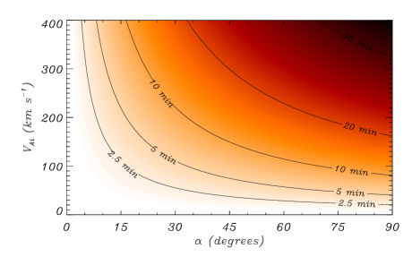
Figure 4.— Growth time $\tau_{g}=1/\gamma_{m}$ of the MRT unstable mode at a single interface as a function of the shear angle $\alpha$ and $V_{Ai}$ for $\chi=1$ and $\zeta=100$.

It is interesting to study the dependence of the growth time, defined as $\tau_{g}=1/\gamma_{m}$, on the equilibrium parameters. In Fig. 4 the two-dimensional dependence of $\tau_{g}$ is represented as a function of $\alpha$ and $\chi$ for $\zeta=100$. We do see that a given growth time can be obtained by the proper combination of the parameters $\alpha$, $\chi$, and $V_{Ai}$. Note that, for small angles, a larger Alfvén speed is required to obtain the same growth rate. In fact, Eq. (35) is further simplified if we take the limit of small shear angles ($\alpha\ll 1$),

$$\gamma_{m}\approx\frac{g|\zeta-1|}{2\alpha V_{Ai}}\sqrt{\frac{\chi^{2}+1}{\zeta(\zeta+1)}}.$$ (36)

This expression explains why decreasing $\alpha$ while keeping $\gamma_{m}$ constant requires an increase of the internal Alfvén speed (if the rest of the parameters, i.e., $g$, $\chi$ and $\zeta$ are constant). In the opposite limit, i.e., when $\alpha\approx\pi/2$, Eq. (35) reduces to

$$\gamma_{m}\approx\frac{g}{2V_{Ai}}\frac{|\zeta-1|}{\sqrt{\zeta\left({\zeta+1}\right)}}\Theta.$$ (37)

where

$$\Theta=\left\{\begin{array}[]{cl}\chi,&\chi>1,\vspace*{2mm}\\ 1,&\chi\leq 1.\end{array}\right.$$ (38)

Thus, as Fig. 4 indicates, for configurations with a strong shear the curve of the growth time is almost horizontal since, according to Eq. (37), it is independent of $\alpha$. Note that for $\chi<1$ the growth time is independent of $\chi$ while it is linearly proportional to $\chi$ for $\chi>1$. Finally note that the factor that contains the dependence with $\zeta$ in the previous expressions is approximately 1 in the limit of $\zeta\gg 1$. Then Eqs. (35)-(37) can be further simplified for configurations with a high density contrast.

4.2. Stability of a magnetic slab

Since now there is a natural spatial scale $a$, it is convenient to introduce a new dimensionless wave number $\kappa=ak$. We also introduce the parameter characterising the relative strength of magnetic field and gravity, $\sigma=V_{Ae}^{2}/(ag)$. Otherwise we use the same dimensionless parameters as in the previous section. Then we rewrite Eq. (24) as

$$\omega_{\pm}^{2}=\frac{g(\tilde{F}\pm\tilde{G})}{a\tilde{H}},$$ (39)

where

$$\tilde{F} = \sigma\kappa^{2}\big{\{}\big{[}\chi^{2}\cos^{2}\varphi+\zeta\cos^{2}(\varphi-\alpha)\big{]}\cosh 2\kappa$$ (40)

$$+ \big{[}\zeta\chi^{2}\cos^{2}\varphi+\cos^{2}(\varphi-\alpha)\big{]}\sinh 2\kappa\},$$

$$\tilde{G} = \Big{\{}\sigma^{2}\kappa^{4}\big{[}\chi^{2}\cos^{2}\varphi-\zeta\cos^{2}(\varphi-\alpha)\big{]}^{2}$$ (41)

$$+ \kappa^{2}(\zeta-1)^{2}\big{[}(\zeta^{2}+1)\sinh^{2}2\kappa+\zeta\sinh 4\kappa\big{]}\Big{\}}^{1/2},\hphantom{xx}$$

$$\tilde{H}=2\zeta\cosh 2\kappa+(\zeta^{2}+1)\sinh 2\kappa.$$ (42)

It is obvious that only $\omega_{-}^{2}$ can be negative, while $\omega_{+}^{2}$ is always positive. Hence, only the sausage perturbations can be unstable, while the kink perturbations are always stable. If $\omega_{-}^{2}<0$, then the two roots of Eq. (23) considered as a quadratic equation with respect to $\omega^{2}$ have different signs. This is only possible when the free term of the quadratic Eq. (23) is negative. In the dimensionless variables this condition is written as

$$\kappa^{2}\sigma^{2}\big{\{}2\chi^{2}\cos^{2}\varphi\cos^{2}(\varphi-\alpha) + \big{[}\cos^{4}(\varphi-\alpha)$$

$$+\,\chi^{4}\cos^{4}\varphi\big{]}\tanh 2\kappa\big{\}} < (\zeta-1)^{2}\tanh 2\kappa.$$ (43)

This inequality can be rewritten as

$$f(\kappa)\equiv\kappa(X+Y\tanh 2\kappa])-Z\frac{\tanh 2\kappa}{\kappa}<0,$$ (44)

where

$$\begin{array}[]{l}X=2\chi^{2}\cos^{2}\varphi\cos^{2}(\varphi-\alpha),\vspace*{1.5mm}\\ Y=\cos^{4}(\varphi-\alpha)+\chi^{4}\cos^{4}\varphi,\vspace*{1.5mm}\\ Z=\sigma^{-2}(\zeta-1)^{2}.\end{array}$$ (45)

Differentiating the function $f(\kappa)$ we obtain

$$f^{\prime}(\kappa)=X+Y\tanh 2\kappa+\frac{2\kappa Y}{\cosh^{2}2\kappa}+\frac{Z[\sinh(4\kappa)-4\kappa]}{2\kappa^{2}\cosh^{2}2\kappa}.$$ (46)

It follows from a well-known inequality $\sinh x>x$ for $x>0$ that the last term on the right-hand side of this equation is positive. Hence, $f^{\prime}(\kappa)>0$. We also have $f(\kappa)\to-2Z<0$ as $\kappa\to 0$ and $f(\kappa)\to\infty$ as $\kappa\to\infty$. This implies that there is exactly one number $\kappa_{c}(\varphi)$ such that $f(\kappa_{c})=0$. The quantity $\kappa_{c}(\varphi)$ is defined by the equation obtained from Eq. (43) by substituting the sign “$<$” by “$=$”. The inequality (43) is satisfied when $\kappa<\kappa_{c}(\varphi)$, and it is not satisfied otherwise. All perturbations with $\kappa>\bar{\kappa}_{c}=\max\kappa_{c}(\varphi)$ are stable. In general, we failed to calculate $\max\kappa_{c}(\varphi)$ analytically, so it must be done numerically.

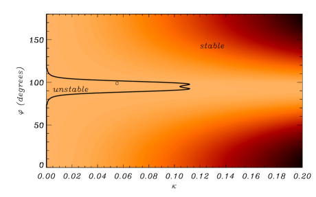
Figure 5.— Square of the frequency (in arbitrary inits) as a function of $\kappa$ and $\varphi$ for the slab problem. The continuous curve corresponds to $\omega^{2}=0$ and represents the transition between stable and MRT unstable modes. The circle indicates the position in the diagram of the maximum growth rate. In this plot, $\alpha=10^{\circ}$, $\chi=1$, $\zeta=100$, $\sigma=3.65\times 10^{4}$.

Figure 6.— Eigenfunction for the $\omega_{-}^{2}$ solution (top panel) and for the stable $\omega_{+}^{2}$ solution (bottom panel) in the slab model. The continuous curve corresponds to an angle of propagation $\varphi=80^{\circ}$, the dotted curve to $\varphi=90^{\circ}$, and the dashed-dot to $\varphi=100^{\circ}$. A fixed dimensionless wave number $\kappa=0.07$ has been selected to calculate the eigenfunctions. The rest of the parameters are the same as in Fig. 5. The vertical dashed lines represent the slab boundaries. Note that some parts of the dotted and dashed-dotted lines are superimposed on the solid lines and therefore not easy to distinguish. This happens on the left part of the top panel and on the right part of the bottom panel.

An example of the dependence of the square of the frequency on $\kappa$ and $\varphi$ is shown in Fig. 5. The value of $\sigma=3.65\times 10^{4}$ used to plot this figure can be obtained if we take, for example, $V_{Ae}=10^{3}$ km s^-1 and $a=100$ km. It is interesting to compare this figure with the results for the single interface shown in Fig. 3. The equilibrium parameters are exactly the same in the two plots, but now for the slab problem we have an additional parameter, which is the half width of the slab, denoted by $a$. The curve representing the transition between the stable and the unstable regime of the $\omega_{-}^{2}$ solution is slightly more complex for the slab problem and shows a double lobe structure around the maximum $\kappa$. The eigenfunctions for three different propagation angles are plotted in Fig. 6 for a fixed $\kappa$ and the same parameters as in Fig. 5. In the top panel the $\omega_{-}^{2}$ solution changes from stable (continuous curve) with a clear “sausage” character to unstable (dotted and dashed-dotted lines). Note that eventually the eigenfunction of this mode is now localised at the lower interface. On the contrary, the solution corresponding to the $\omega_{+}^{2}$, see bottom panel of Fig. 6, has a clear “kink” profile, but it tends to be localised at the upper interface when $\varphi$ is increased. Therefore the nature of the modes is closer to surface waves associated to the individual interfaces. Similar results were found in Terradas et al. (2012) in the absence of magnetic shear.

We concentrate now on the analysis of the growth time. In Fig. 7 the dependence of $\tau_{g}$ associated to the most unstable mode is plotted as a function of $\alpha$ and $V_{Ai}$ for a fixed value of $\chi$, $\zeta$, and $a$. The differences with respect to the interface results, see Fig. 4, are that the curves of constant $\tau_{g}$ have essentially shifted down in the diagram. This means that the slab configuration is more stable than the interface model. This diagram can be used as a diagnostic tool and clearly shows the dependence of the grow times in the space of parameters.

Figure 7.— Growth time of the MRT instability for the slab problem as a function of the shear angle $\alpha$ and $V_{Ai}$. In this plot $\chi=1$, $\zeta=100$ and $a=100\,\rm km$.

The stability analysis is greatly simplified in two limiting cases. In the fist case the magnetic fields in the slab and external regions are almost parallel, $\alpha\ll 1$, and $|\zeta-1|/\sigma$ is of the order of unity. In this case it follows from the equation $f(\kappa)=0$ that $\kappa_{c}(\varphi)$ takes moderate values when $\varphi$ is not close to $\pi/2$, while it takes very large values when $\varphi$ is close to $\pi/2$. Hence, to calculate $\bar{\kappa}_{c}$, it is enough to consider $\varphi$ close to $\pi/2$. In accordance with this we put $\varphi=\pi/2-\psi$ and assume that $|\psi|\ll 1$. In addition, since $\kappa_{c}\gg 1$, we can take $\tanh 2\kappa_{c}\approx 1$. Then we obtain from the equation $f(\kappa)=0$ the approximate expression

$$\kappa_{c}(\varphi)\approx\frac{|\zeta-1|}{\sigma[(\psi+\alpha)^{2}+\chi^{2}\psi^{2}]}.$$ (47)

It immediately follows that

$$\bar{\kappa}_{c}=\kappa_{c}(\varphi_{c})\approx\frac{|\zeta-1|(1+\chi^{2})}{\sigma\chi^{2}\alpha^{2}},\quad\varphi_{c}\approx\frac{\pi}{2}+\frac{\alpha}{1+\chi^{2}}.$$ (48)

It is also not difficult to obtain the asymptotic expression for $\omega_{-}^{2}$ valid for $\alpha\ll 1$ and $|\varphi-\pi/2|\ll 1$. It is given by

$$\omega_{-}^{2}\approx\frac{g\{\sigma\kappa^{2}[\chi^{2}\psi^{2}+(\psi+\alpha)^{2}]-\kappa|\zeta-1|\}}{a(\zeta+1)}.$$ (49)

When deriving this expression we have assumed that $\kappa\gg 1$ because $|\omega_{-}^{2}|$ is of the order of $g/a$ when $\kappa\sim 1$, while $|\omega_{-}^{2}|\gg g/a$ when $\kappa\gg 1$. The quantity $\omega_{-}^{2}$ takes its minimum value at $\varphi=\varphi_{c}$ and $\kappa=\frac{1}{2}\bar{\kappa}_{c}$, and the maximum growth rate is given by

$$\gamma_{m}\approx\frac{|\zeta-1|}{2\chi\alpha}\sqrt{\frac{g(1+\chi^{2})}{a\sigma(\zeta+1)}}.$$ (50)

In terms of the internal Alfvén speed the previous expression reduces to

$$\gamma_{m}\approx\frac{g|\zeta-1|}{2\alpha V_{Ai}}\sqrt{\frac{\chi^{2}+1}{\zeta(\zeta+1)}}.$$ (51)

This is exactly the same as Eq. (36) which corresponds to the interface result in the limit of small $\alpha$. This confirms that the slab problem in the limit of $\kappa\gg 1$ reduces to the interface problem because the penetration scale given by $1/\kappa$ is rather small and the role of the upper interface is negligible for the unstable mode (see also the plot of the eigenfunctions in Fig. 6). Again we see that the situation here is similar to one that we have in the case of a single interface: $\gamma_{m}\to\infty$ as $\alpha\to 0$, so, in the case of parallel magnetic field ($\alpha=0$), the growth rate is unbounded and the initial value problem is ill-posed. On the other hand, the growth rate is bounded when the magnetic field is sheared ($\alpha\neq 0$), so the initial value problem is well-posed. As mentioned in the case of a single interface, the growth rate of the MRT instability in the model with parallel magnetic field ($\alpha=0$) will be bounded and the problem will be well-posed if we take into account either dissipation or the finite thickness of the transitions between the three homogeneous regions.

Another limiting case where the analytic asymptotic analysis is possible is when $\zeta\gg 1$ and $\sigma\gtrsim\zeta^{2}$, while $\chi\simeq 1$ and $\alpha\simeq 1$. In this case it is not difficult to see from the equation $f(\kappa)=0$ that $\kappa_{c}(\varphi)\ll 1$, so the equation $f(\kappa)=0$ can be written in the approximate form as

$$\kappa^{2}\big{[}\cos^{4}(\varphi - \alpha)+\chi^{4}\cos^{4}\varphi\big{]}$$ (52)

$$+ \kappa\chi^{2}\cos^{2}\varphi\cos^{2}(\varphi-\alpha)=\zeta^{2}\sigma^{-2}.$$

This equation is used in Appendix A to calculate $\varphi_{c}$. It is found that

$$\begin{array}[]{l}\displaystyle\varphi_{c}=\varphi_{c1}\approx\frac{\pi}{2}+\frac{2\zeta\cot\alpha}{\sigma\chi^{2}},\vspace*{2mm}\\ \displaystyle\bar{\kappa}_{c}=\kappa_{c}(\varphi_{c1})\approx\frac{\zeta}{\sigma\sin^{2}\alpha}\end{array}$$ (53)

when $\chi>1$ and

$$\begin{array}[]{l}\displaystyle\varphi_{c}=\varphi_{c2}\approx\frac{\pi}{2}+\alpha-\frac{2\zeta\cot\alpha}{\sigma},\vspace*{2mm}\\ \displaystyle\bar{\kappa}_{c}=\kappa_{c}(\varphi_{c2})\approx\frac{\zeta}{\sigma\chi^{2}\sin^{2}\alpha}\end{array}$$ (54)

when $\chi<1$.

Figure 8.— The dependence of $s_{c}$ on $\Delta$.

Figure 9.— The dependence of $\Gamma$ on $\Delta$.

It is shown in Appendix B that the fastest growing mode propagates approximately perpendicular to the external magnetic field ($\varphi\approx\pi/2+\alpha$). Its dimensionless wave number is equal to $\kappa_{c}=\zeta^{-1}s_{c}(\Delta)$, where

$$\Delta=\frac{\sigma\chi^{2}\sin^{2}\alpha}{\zeta^{2}}.$$ (55)

The dependence of $s_{c}$ on $\Delta$ is shown in Fig. 8. The instability increment is equal to

$$\gamma_{m}=(g/a\zeta)^{1/2}\Gamma(\Delta).$$ (56)

The dependence of $\Gamma$ on $\Delta$ is plotted in Fig. 9. All these results are obtained under the assumption that $\zeta\Delta>1$, i.e., when $\chi^{2}\sin^{2}\alpha>\zeta/\sigma$.

In Fig. 10 the growth time of the instability calculated using the full solution (continuous curve) is plotted together with the approximation for finite angles (dashed curves) given by Eq. (56). We do see a good match in the behaviour of the two curves. The approximation slightly underestimates the growth time, and the differences increase when $\sigma$ decreases. This is what we should expect if we recall that the approximation is based on the assumption $\sigma\gg 1$. We have already shown that, for small angles of the shear, the interface and the slab results are the same. Now this is also evident in Fig. 10. This plot also shows that the differences in the growth time between the slab and the interface can be quite significant for $\alpha\simeq 1$.

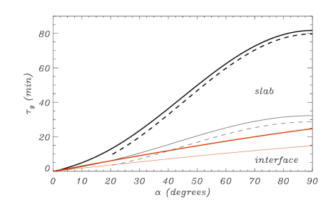
Figure 10.— Growth time of the MRT instability for the slab problem (black colour) and interface problem (red colour) as a function of the shear angle $\alpha$. The thin curves correspond to $\sigma=1.45\times 10^{5}$ ($V_{Ai}=200\rm\,km\,s^{-1}$) while thick curves represent the case $\sigma=5.2\times 10^{4}$ ($V_{Ai}=120\rm\,km\,s^{-1}$). Dashed lines correspond to the approximation in the slab problem for large angles given by Eq. (56). In this plot $\chi=1$ and $\zeta=100$.

5. Application to oscillating threads

The purpose of this section is to use the previous theoretical results to infer some information about the shear in real prominence threads. We consider the thread oscillation studied by Okamoto et al. (2007) using HINODE. These authors found threads oscillating vertically with periods around 4 min. Terradas et al. (2008) used these oscillations to do a seismological study of the thread. Although Okamoto et al. (2007) did not investigate the lifetime of the threads, from the movie of the event we estimate that threads do not last long. It is found that the typical lifetime is 10 min. The main idea here is to assume that the excitation of nstable modes is responsible for the short lifetime of the structure. This MRT instability produces the disappearance of the structure. According to our results the fastest growing mode when there is magnetic shear has the following approximate growth time (see Eq. (36))

$$\tau_{g}\approx\frac{\sqrt{2}}{g}V_{Ai}\alpha,$$ (57)

where we have assumed that $\zeta\gg 1$ and $\chi\approx 1$. This expression applies to the interface problem as well as to the slab problem (see Eq. (51)), and it is valid in the limit of small $\alpha$ only. If the growth time is assumed to be around $10\rm\,min$ in order to use Eq. (57) we must obtain a small angle, otherwise we get an inconsistent result. Terradas et al. (2008) found that the lower bound for the internal Alfvén speed is between 120 and $350\,\rm km\,s^{-1}$. Nevertheless, some of the threads have high Alfvén velocities, up to $800\,\rm kms^{-1}$, since they belong to an active region prominence. Let us assume that the velocity is around $500\,\rm km\,s^{-1}$ and calculate the corresponding shear angle. According to Eq. (57) and using that $\tau_{g}=10\,\rm min$ and $V_{Ai}=500\,\rm km\,s^{-1}$ we obtain that $\alpha\approx 13^{\circ}$. This angle is small and the application of Eq. (57) is justified. This is in agreement with the behaviour found in the more general expression given by Eq. (35) which shows that $\alpha$ decreases when the internal Alfvén speed increases (see also Fig. 4). In fact this expression shows that $\alpha$ is small for sufficiently large values of $V_{Ai}$ but moderate for smaller values. For the present case of a velocity of $V_{Ai}=500\,\rm km\,s^{-1}$ the angle is small, and this is in accordance with the observations of prominence threads.

The observed oscillations of the thread are most probably kink oscillations. It is well known that the sausage waves in magnetic slabs and and tubes have quite similar properties, while the properties of kink waves in slabs are quite different from those in tubes (e.g. Edwin & Roberts, 1982, 1983). Since $\omega_{+}$-mode is a kink mode, it is quite improbable that the observed oscillations of the thread are described by this mode. Note that, in the linear approximation, the kink oscillation of the thread does not interact with the unstable mode causing its disappearance, and thus it does not affect the instability growth time.

6. Summary and conclusions

In the present paper we have extended the study by Terradas et al. (2012) to the models of an interface and a slab with magnetic shear, and have focused on the MRT instability. The fact that the magnetic field changes its direction introduces a bounded growth rate of the instability. This is different from the models without shear where the growth rate is unbounded. Because of this Terradas et al. (2012) concentrated on a particular wave number in the perpendicular direction equal to $1/a$, $a$ being the half-thickness of the slab. Here we have focused on the maximum growth rate, representing the most unstable mode of the system, and have found analytical expressions in various limiting cases. For small angles of the shear the growth time is linearly proportional to the shear angle $\alpha$. This applies to the single interface as well as to the slab problem. On the contrary, for large angles the growth time depends only weakly on $\alpha$ in the interface problem. In this limit, we have also been able to calculate an approximate expression for the growth time in the slab problem.

We have shown, using a simple example, how it is possible to estimate the shear angle in threads belonging to active region prominences from the combination of observations and the theoretical results presented in this paper. Using this method we have found that the observations of oscillating threads of Okamoto et al. (2007) are compatible with small shear angles (around $13^{\circ}$). This indirect method of inferring some of the equilibrium properties of threads can be potentially used as a seismological tool.

Several simplifications have been done in the models considered in this work. Both the interface and slab configurations are unbounded in the perpendicular direction ($y$-direction) and we have assumed that there is dense material along the full length of the magnetic tube. However, in reality, threads only represent a small part of the full magnetic tube. Compressibility and partial ionisation (see Díaz et al., 2012) have been also ignored. These basic assumptions in the models have enabled us to derive analytical expressions for the growth times. Nevertheless, the need for using improved models is obvious, and the study of the nonlinear evolution of the system is very relevant to asses the role of the MRT instability in the fast disappearance of threads.

Acknowledgements. A part of this work was carried out when MSR was a guest of Departament de Física of Universitat de les Illes Balears. He acknowledges the financial support received from the Universitat de les Illes Balears and the warm hospitality of the Departament. He also acknowledges the support by the STFC grant. J.T. acknowledges support from the Spanish Ministerio de Educación y Ciencia through a Ramón y Cajal grant and financial support from MICINN/MINECO and FEDER Funds through grant AYA2011-22846 Funding from CAIB through the Grups Competitius scheme and FEDER Funds is also acknowledged.

Appendix A Calculation of $\varphi_{c}$ and $\bar{\kappa}_{c}$ for the slab model.

In this appendix we calculate $\varphi_{c}$ and $\bar{\kappa}_{c}$ for the slab model in the case where $\sigma\gg\zeta\gg 1$, while $\chi\simeq 1$ and $\alpha\simeq 1$. As it is shown in Sect. 4.2, in this case $\kappa_{c}(\varphi)$ is defined by the approximate Eq. (52). To calculate $\varphi_{c}$ we differentiate Eq. (52) with respect to $\varphi$ and then take $d\kappa/d\varphi=0$. As a result we obtain

$$2\kappa\big{[}\chi^{4}\cos^{3}\varphi\sin\varphi + \cos^{3}(\varphi-\alpha)\sin(\varphi-\alpha)\big{]}$$ (A1)

$$+ \chi^{2}\cos\varphi\cos(\varphi-\alpha)\sin(2\varphi-\alpha)=0.$$

Eliminating $\kappa$ from this equation and Eq. (52) we obtain the equation for $\varphi_{c}$:

$$\sin\alpha\cos^{2}\varphi\cos^{2}(\varphi-\alpha)\sin(2\varphi-\alpha)\big{[}\cos^{4}(\varphi\!\! - \!\!\alpha)-\chi^{4}\cos^{4}\varphi\big{]}$$

$$=\zeta^{2}\sigma^{-2}\chi^{-4}\big{\{}\cos^{2}(\varphi-\alpha)\sin[2(\varphi-\alpha)]\!\! + \!\!\chi^{4}\cos^{2}\varphi\sin 2\varphi\}^{2}.$$ (A2)

Since $\zeta^{2}\sigma^{-2}\ll 1$, to obtain the solution to this equation we use the regular perturbation method. In the first-order approximation we obtain that the left-hand side of Eq. (A2) is zero. It is possible when one of the four multiplier that depend on $\varphi$ is zero. We investigate these possibilities separately.

(i) Let $\cos\varphi=0$, i.e. $\varphi=\pi/2$. In the second-order approximation we look for the solution in the form $\varphi=\pi/2-\psi$, where $|\psi|\ll 1$. Substituting this expression in Eq. (A2) we easily calculate $\psi$ and eventually obtain

$$\varphi_{1\pm}\approx\frac{\pi}{2}\pm\frac{2\zeta\cot\alpha}{\sigma\chi^{2}}.$$ (A3)

(ii) Let $\cos(\varphi-\alpha)=0$, i.e. $\varphi=\pi/2+\alpha$. In the second-order approximation we look for the solution in the form $\varphi=\pi/2+\alpha-\psi$, where $|\psi|\ll 1$. Substituting this expression in Eq. (A2) we, once again, easily calculate $\psi$ and obtain

$$\varphi_{2\pm}\approx\frac{\pi}{2}+\alpha\pm\frac{2\zeta\cot\alpha}{\sigma}.$$ (A4)

(iii) Let $\sin(2\varphi-\alpha)=0$, i.e. $\varphi=\frac{1}{2}\alpha$ or $\varphi=(\pi+\alpha)/2$. In the second-order approximation we look for the solution in the form $\varphi=\frac{1}{2}\alpha+\psi$, where $|\psi|\ll 1$. Substituting this expression in Eq. (A2) we calculate $\psi$ and obtain

$$\varphi_{3}\approx\frac{\alpha}{2}+\frac{2\zeta^{2}(1-\chi^{4})}{\sigma^{2}\chi^{4}}\tan\frac{\alpha}{2}\,{\rm sec}^{3}\frac{\alpha}{2}.$$ (A5)

Similarly, looking for the solution in the form $\varphi=(\pi+\alpha)/2+\psi$ with $|\psi|\ll 1$, we obtain

$$\varphi_{4}\approx\frac{\pi}{2}\ +\frac{\alpha}{2}+\frac{2\zeta^{2}(\chi^{4}-1)}{\sigma^{2}\chi^{4}}\cot\frac{\alpha}{2}\,{\rm cosec}^{3}\frac{\alpha}{2}.$$ (A6)

(iv) Let $\cos(\varphi-\alpha)=\pm\chi\cos\varphi$. It follows from this equation that

$$\varphi=\varphi_{0}\equiv\arctan\frac{\pm\chi-\cos\alpha}{\sin\alpha}.$$ (A7)

In the second-order approximation we look for the solution in the form $\varphi=\varphi_{0}+\psi$, where $|\psi|\ll 1$. Substituting this expression in Eq. (A2), after some algebra, we obtain in the second-order approximation

$$\psi\sin\alpha\sin(2\varphi_{0}\!\! - \!\!\alpha)[\pm\chi\sin\varphi_{0}-\sin(\varphi_{0}-\alpha)]$$ (A8)

$$= \!\zeta^{2}\sigma^{-2}\chi^{-6}[\tan\varphi_{0}(\cos\alpha\pm\chi)-\sin\alpha]^{2}.$$

Using Eq. (A7) we derive the formulae

$$\begin{array}[]{c}\displaystyle\sin(2\varphi_{0}-\alpha)=\frac{\sin\alpha(\chi^{2}-1)}{1\mp 2\chi\cos\alpha+\chi^{2}},\vspace*{2mm}\\ \pm\chi\sin\varphi_{0}-\sin(\varphi_{0}-\alpha)=\sqrt{1\mp 2\chi\cos\alpha+\chi^{2}}.\end{array}$$ (A9)

With the aid of Eqs. (A7) and Eq. (A9) we calculate $\psi$ from Eq. (A8). Finally we obtain

$$\varphi_{5\pm}\approx\arctan\frac{\pm\chi-\cos\alpha}{\sin\alpha}+\frac{\zeta^{2}(\chi^{2}-1)\sqrt{1\mp 2\chi\cos\alpha+\chi^{2}}}{\sigma^{2}\chi^{6}\sin^{4}\alpha}.$$ (A10)

Hence, we have eight values of $\varphi$ that are the solutions of Eq. (52), and we have to choose one at that $\kappa_{c}(\varphi)$ takes its maximum value. To do this we have to calculate $\kappa_{c}(\varphi)$ at each of these eight values of $\varphi$ using Eq. (A1). The calculation is lengthy but straightforward, so we give only the final results:

$$\begin{array}[]{c}\displaystyle\kappa_{c}(\varphi_{1\pm})\approx\frac{\pm\zeta}{\sigma\sin^{2}\alpha},\quad\kappa_{c}(\varphi_{2\pm})\approx\frac{\mp\zeta}{\sigma\chi^{2}\sin^{2}\alpha},\vspace*{2mm}\\ \displaystyle\kappa_{c}(\varphi_{3})\approx\frac{2\zeta^{2}}{\sigma^{2}\chi^{2}}\,\mbox{sec}^{5}\frac{\alpha}{2},\vspace*{2mm}\\ \displaystyle\kappa_{c}(\varphi_{4})\approx\frac{2\zeta^{2}}{\sigma^{2}\chi^{2}}\,\mbox{cosec}^{5}\frac{\alpha}{2},\quad\kappa_{c}(\varphi_{5\pm})\approx-\frac{1}{2}.\end{array}$$ (A11)

We disregard negative values of $\kappa_{c}$ because we assumed from the very beginning that $\kappa>0$. Since we have assumed that $\zeta/\sigma\ll 1$, it is straightforward to see that $\kappa_{c}(\varphi_{1+})>\kappa_{c}(\varphi_{3}),\,\kappa_{c}(\varphi_{4})$ and $\kappa_{c}(\varphi_{2-})>\kappa_{c}(\varphi_{3}),\,\kappa_{c}(\varphi_{4})$. Hence, eventually,

$$\bar{\kappa}_{c}\approx\kappa_{c}(\varphi_{1+})\approx\frac{\zeta}{\sigma\sin^{2}\alpha},\quad\chi>1,$$ (A12)

and

$$\bar{\kappa}_{c}\approx\kappa_{c}(\varphi_{2-})\approx\frac{\zeta}{\sigma\chi^{2}\sin^{2}\alpha},\quad\chi<1.$$ (A13)

Appendix B Calculation of maximum increment.

In this this section we calculate the maximum growth rate of the Rayleigh-Taylor instability. In accordance with Eq. (A1) the dimensionless wave number of an unstable mode is always small, $\kappa\lesssim\zeta/\sigma\ll 1$. This observation enables us to use the approximate Taylor expansions with respect to $\kappa$ for functions $\tilde{F}$, $\tilde{G}$ and $\tilde{H}$:

$$\tilde{F} = \sigma\kappa^{2}\big{\{}\big{[}\chi^{2}\cos^{2}\varphi+\zeta\cos^{2}(\varphi-\alpha)\big{]}\big{(}1+2\kappa^{2}\big{)}$$ (B1)

$$+ 2\kappa\big{[}\zeta\chi^{2}\cos^{2}\varphi+\cos^{2}(\varphi-\alpha)\big{]}\big{\}},$$

$$\tilde{G}=\Big{\{}\sigma^{2}\kappa^{4}\big{[}\chi^{2}\cos^{2}\varphi-\zeta\cos^{2}(\varphi-\alpha)\big{]}^{2}+4\kappa^{3}\zeta^{3}(1+\zeta\kappa)\Big{\}}^{1/2},$$ (B2)

$$\tilde{H}=2\zeta(1+\zeta\kappa).$$ (B3)

We introduce the dimensionless increment $\tilde{\gamma}=(g/a)^{1/2}|\omega_{-}|$. Then we obtain from Eq. (39) the approximate equation

$$\tilde{\gamma}^{2}=2\kappa^{3}\frac{\zeta^{2}-\sigma^{2}\kappa\{\kappa[\chi^{4}\cos^{4}\varphi+\cos^{4}(\varphi-\alpha)]+\chi^{2}\cos^{2}\varphi\cos^{2}(\varphi-\alpha)\}}{\tilde{F}+\tilde{G}}.$$ (B4)

Now we investigate this expression in three various intervals of variation of the angle $\varphi$.

(i) Let $\cos^{2}\varphi\simeq\cos^{2}(\varphi-\alpha)\simeq 1$, i.e. $\varphi$ be not close to $\pi/2$ and to $\pi/2+\alpha$. Then it follow from Eq. (B4) that $\tilde{\gamma}^{2}>0$ only when $\kappa\lesssim\zeta^{2}/\sigma^{2}$. For these values of $\kappa$ we have $\tilde{F}+\tilde{G}\gtrsim\zeta^{5}/\sigma^{3}$ and $\tilde{\gamma}\lesssim(\zeta/\sigma)^{3/2}$.

(ii) Let $\varphi$ be close to $\pi/2$, so we take $\varphi=\pi/2-\tilde{\varphi}$. Then we can use the approximate expression

$$\tilde{\gamma}^{2}\approx 2\kappa^{2}\frac{\zeta^{2}-\sigma^{2}\kappa\sin^{2}\alpha(\kappa\sin^{2}\alpha+\chi^{2}\tilde{\varphi}^{2})}{\sigma\zeta\kappa\sin^{2}\alpha+\zeta(\sigma^{2}\kappa^{2}\sin^{2}\alpha+4\zeta\kappa)^{1/2}},$$ (B5)

It is obvious that, for any fixed $\kappa$, $\tilde{\gamma}^{2}$ takes its maximum value at $\tilde{\varphi}=0$. When $\kappa\lesssim\zeta/\sigma^{2}$, we obtain $\tilde{\gamma}^{2}\simeq\zeta^{2}/\sigma^{3}\ll\zeta^{2}/\sigma^{2}$. On the other hand, we obtain $\tilde{\gamma}^{2}\simeq\zeta^{2}/\sigma^{2}$ when $\kappa\simeq\zeta/\sigma$. Hence, when looking for the maximum value of $\tilde{\gamma}$, we can take $\tilde{\varphi}=0$ and $\kappa\simeq\zeta/\sigma$. In that case $\sigma^{2}\kappa^{2}\sin^{2}\alpha\gg 4\zeta\kappa$ and we can further reduce Eq. (B5) to

$$\tilde{\gamma}^{2}\approx\frac{\kappa(\zeta^{2}-\sigma^{2}\kappa^{2}\sin^{4}\alpha)}{\sigma\zeta\sin^{2}\alpha}.$$ (B6)

Then we easily find that the maximum value of $\tilde{\gamma}$ is given by

$$\tilde{\gamma}_{m}\approx\frac{\zeta}{\sigma\sin^{2}\alpha}\sqrt[4]{\frac{4}{27}},$$ (B7)

and it is taken at

$$\kappa\approx\frac{\zeta}{\sqrt{3}\sigma\sin^{2}\alpha}.$$ (B8)

(iii) Let now $\varphi$ be close to $\pi/2+\alpha$, so we take $\varphi=\pi/2+\alpha-\tilde{\varphi}$. Then we can use the approximate expression

$$\tilde{\gamma}^{2}\approx 2\kappa^{3}\frac{\zeta^{2}-\sigma^{2}\kappa\chi^{2}\sin^{2}\alpha(\kappa\chi^{2}\sin^{2}\alpha+\tilde{\varphi}^{2})}{\tilde{F}+\tilde{G}},$$ (B9)

where $\tilde{F}$ and $\tilde{G}$ are given by

$$\tilde{F}\approx\sigma\kappa^{2}\left[\chi^{2}\sin^{2}\alpha(1+2\zeta\kappa)+\zeta\tilde{\varphi}^{2}\right],$$ (B10)

$$\tilde{F}\approx\left[\sigma^{2}\kappa^{4}(\chi^{2}\sin^{2}\alpha-\zeta\tilde{\varphi}^{2})^{2}+4\zeta^{3}\kappa^{3}(1+\zeta\kappa)\right]^{1/2}.$$ (B11)

It is easy to show that $\tilde{F}+\tilde{G}$ is a monotonically increasing function of $\tilde{\varphi}^{2}$. Since the numerator in Eq. (B9) is a monotonically decreasing function of $\tilde{\varphi}^{2}$, we conclude that, at a fixed $\kappa$, $\tilde{\gamma}$ takes its maximum value at $\tilde{\varphi}=0$. Hence, we can take

$$\tilde{\gamma}^{2}\approx\frac{2\kappa^{2}(\zeta^{2}-\sigma^{2}\kappa^{2}\chi^{2}\sin^{4}\alpha)}{\sigma\kappa\chi^{2}\sin^{2}\alpha(1+2\zeta\kappa)+[\sigma^{2}\kappa^{2}\chi^{4}\sin^{4}\alpha+4\kappa\zeta^{3}(1+\zeta\kappa)]^{1/2}}$$ (B12)

when looking for the maximum value of $\tilde{\gamma}$. Introducing the new dimensionless variables

$$s=\zeta\kappa,\quad\Delta=\frac{\sigma\chi^{2}\sin^{2}\alpha}{\zeta^{2}},$$ (B13)

we obtain after some algebra

$$\tilde{\gamma}^{2}=s\frac{[s^{2}\Delta^{2}+4s(1+s)]^{1/2}-s\Delta(1+2s)}{2\zeta(1+s)}.$$ (B14)

To calculate the maximum of function $\tilde{\gamma}^{2}(s)$ we have to find where its derivative is equal to zero. After some algebra the equation $d\tilde{\gamma}^{2}/ds=0$ can be written as

$$2\Delta^{4}(2s^{6}\! + \!7s^{5}+8s^{4}+3s^{3})+\Delta^{2}(16s^{6}+72s^{5}+119s^{4}+84s^{3}$$ (B15)

$$+ \!19s^{2}-2s)-(4s^{4}+20s^{3}+37s^{2}+30s+9)=0.$$

We consider this equation as a quadratic equation for $\Delta^{2}$. The roots of this equation have different signs. Then, taking into account that $\Delta^{2}>0$, we obtain that $s$ is defined by the equation

$$\Upsilon(s)=\Delta^{2},$$ (B16)

where $\Upsilon(s)$ is given by

$$\Upsilon(s) = [s^{2}(2s^{3}+7s^{2}+8s+3)]^{-1}\big{[}(256s^{10}+2304s^{9}$$ (B17)

$$+ 9056s^{8}+20368s^{7}+28833s^{6}+26592s^{5}$$

$$+ 15962s^{4}+6028s^{3}+1321s^{2}+140s+4)^{1/2}$$

$$- (16s^{5}+72s^{4}+119s^{3}+84s^{2}+19s-2)\big{]}.$$

It is straightforward to obtain that $\Upsilon(s)\to\infty$ as $s\to 0$ and $\Upsilon(s)\to 0$ as $s\to\infty$. We verified numerically that $\Upsilon(s)$ is a monotonically decreasing function. Hence, Eq. (B16) has the single solution $s_{c}$ for any value of $\Delta$. The dependence of $s_{c}$ on $\Delta$ is shown in Fig. 8.

Since $\tilde{\gamma}^{2}(0)=0$ and $\tilde{\gamma}^{2}(s)\to-\infty$ as $s\to\infty$ and it has only one extremum at $s=s_{c}$, this extremum is the maximum, i.e. $\tilde{\gamma}_{m}=\tilde{\gamma}(s_{c})$. The dependence of $\Gamma=\zeta^{1/2}\tilde{\gamma}_{n}$ on $\Delta$ is shown in Fig. 9.

Summarising the analysis we see that the function $\tilde{\gamma}(\varphi,\kappa)$ has two local maxima. The first one is given by Eq. (B7) and it is taken at $\varphi=\pi/2$ and $\kappa$ given by Eq. (B8). The second local maximum is given by Eq. (B14) with $s=s_{c}$, and it is taken at $\varphi=\pi/2+\alpha$ and $\kappa=\zeta^{-1}s_{c}$, where $s_{c}$ is defined by Eq. (B16). We temporarily denote the first local maximum as $\tilde{\gamma}_{m1}$ and the second as $\tilde{\gamma}_{m2}$. The absolute maximum of $\tilde{\gamma}(\varphi,\kappa)$ is equal to the larger of the two quantities $\tilde{\gamma}_{m1}$ and $\tilde{\gamma}_{m2}$.

Equation (B7) can be rewritten as

$$\tilde{\gamma}_{m1}\approx\frac{\chi^{2}}{\zeta\Delta}\sqrt[4]{\frac{4}{27}}.$$ (B18)

Then it follows that

$$\frac{\tilde{\gamma}_{m1}}{\tilde{\gamma}_{m2}}\approx\frac{\chi^{2}}{\Delta\Gamma(\Delta)\sqrt{\zeta}}\sqrt[4]{\frac{4}{27}}\approx\frac{0.62\chi^{2}}{\Delta\Gamma(\Delta)\sqrt{\zeta}}.$$ (B19)

It is not difficult to obtain the approximate expressions

$$s_{c}\approx\left\{\begin{array}[]{cl}\displaystyle\frac{1}{2\Delta},&\Delta\ll 1,\vspace*{3mm}\\ \displaystyle\frac{1}{\Delta\sqrt{6}},&\Delta\gg 1,\end{array}\right.$$ (B20)

Using this result we obtain

$$\Gamma\approx\left\{\begin{array}[]{cl}\displaystyle\frac{1}{2\sqrt{\Delta}},&\Delta\ll 1,\vspace*{3mm}\\ \displaystyle\frac{1}{\Delta}\sqrt{\frac{5}{6\sqrt{6}}},&\Delta\gg 1,\end{array}\right.$$ (B21)

We verified numerically that $\Delta\Gamma(\Delta)$ is a monotonically increasing function of $\Delta$. Hence, it varies from $0.5\sqrt{\Delta}$ to $(5/6\sqrt{6})^{1/2}$ when $\Delta$ varies from very small value to $\infty$. Then it follows from Eq. (B19) that $\tilde{\gamma}_{m1}/\tilde{\gamma}_{m2}\lesssim\chi^{2}(\zeta\Delta)^{-1/2}$. Hence, we conclude that $\tilde{\gamma}_{m1}\lesssim\tilde{\gamma}_{m2}$ for $\Delta>\chi^{4}/\zeta$. Since we assume that $\chi\simeq 1$, while the typical value of $\zeta$ is 100, we conclude that, for not very small values of $\Delta$ (say, $\Delta\gtrsim 0.1$), the absolute maximum of $\tilde{\gamma}$ is equal to $\tilde{\gamma}_{m2}$, i.e. $\tilde{\gamma}_{m}=\zeta^{-1/2}\Gamma(\Delta)$. It is taken at $\varphi\approx\pi/2+\alpha$ and $\kappa\approx\zeta^{-1}s_{c}(\Delta)$.

References

- Bucciantini et al. (2004) Bucciantini, N., Amato, E., Bandiera, R., Blondin, J. M., & Del Zanna, L. 2004, A&A, 423, 253
- Chandrasekhar (1961) Chandrasekhar, S. 1961, Hydrodynamic and hydromagnetic stability (Oxford: Clarendon Press)
- DeVore (2012) DeVore, C. R. 2012, in American Astronomical Society Meeting Abstracts, Vol. 220, American Astronomical Society Meeting Abstracts 220, 201.06
- DeVore (2013) DeVore, C. R. 2013, in AAS/Solar Physics Division Meeting, Vol. 44, AAS/Solar Physics Division Meeting, …41
- Díaz et al. (2012) Díaz, A. J., Soler, R., & Ballester, J. L. 2012, ApJ, 754, 41
- Edwin & Roberts (1982) Edwin, P. M. & Roberts, B. 1982, Solar Physics, 76, 239
- Edwin & Roberts (1983) Edwin, P. M. & Roberts, B. 1983, Solar Physics, 88, 179
- Goedbloed (1971a) Goedbloed, J. P. 1971a, Physica, 53, 412
- Goedbloed (1971b) Goedbloed, J. P. 1971b, Physica, 53, 501
- Goedbloed (1971c) Goedbloed, J. P. 1971c, Physica, 53, 535
- Goedbloed & Poedts (2004) Goedbloed, J. P. H. & Poedts, S. 2004, Principles of Magnetohydrodynamics (Cambridge, UK: Cambridge University Press)
- Hillier et al. (2012a) Hillier, A., Berger, T., Isobe, H., & Shibata, K. 2012a, ApJ, 746, 120
- Hillier et al. (2011) Hillier, A., Isobe, H., Shibata, K., & Berger, T. 2011, ApJ, 736, L1
- Hillier et al. (2012b) Hillier, A., Isobe, H., Shibata, K., & Berger, T. 2012b, ApJ, 756, 110
- Isobe et al. (2005) Isobe, H., Miyagoshi, T., Shibata, K., & Yokoyama, T. 2005, Nature, 434, 478
- Isobe et al. (2006) Isobe, H., Miyagoshi, T., Shibata, K., & Yokoyama, T. 2006, PASJ, 58, 423
- Jones & De Young (2005) Jones, T. W. & De Young, D. S. 2005, ApJ, 624, 586
- Jun & Norman (1996) Jun, B.-I. & Norman, M. L. 1996, ApJ, 465, 800
- Jun et al. (1995) Jun, B.-I., Norman, M. L., & Stone, J. M. 1995, ApJ, 453, 332
- Okamoto et al. (2007) Okamoto, T. J., Tsuneta, S., Berger, T. E., et al. 2007, Science, 318, 1577
- O’Neill et al. (2009) O’Neill, S. M., De Young, D. S., & Jones, T. W. 2009, ApJ, 694, 1317
- Parker (1974) Parker, E. N. 1974, Solar Physics, 37, 127
- Rayleigh (1883) Rayleigh, L. 1883, Proc. London Math. Soc., 14, 170
- Roberts (1981a) Roberts, B. 1981a, Solar Physics, 69, 27
- Robinson et al. (2004) Robinson, K., Dursi, L. J., Ricker, P. M., et al. 2004, ApJ, 601, 621
- Ryutova et al. (2010) Ryutova, M., Berger, T., Frank, Z., Tarbell, T., & Title, A. 2010, Sol. Phys., 267, 75
- Stone & Gardiner (2007) Stone, J. M. & Gardiner, T. 2007, ApJ, 671, 1726
- Taylor (1950) Taylor, G. I. 1950, Proc. Roy. Soc. London A, 201, 192
- Terradas et al. (2008) Terradas, J., Arregui, I., Oliver, R., & Ballester, J. L. 2008, ApJ, 678, L153
- Terradas et al. (2012) Terradas, J., Oliver, R., & Ballester, J. L. 2012, A&A, 541, A102
- Yang et al. (2011) Yang, B. L., Wang, L. F., Ye, W. H., & Xue, C. 2011, Physics of Plasmas, 18, 072111
- Zhang et al. (2012) Zhang, P., Lau, Y. Y., Rittersdorf, I. M., et al. 2012, Physics of Plasmas, 19, 022703